Article

Distributed Robust Predefined-Time Sliding Mode Control for AUV-USV Heterogeneous Multi-Agent Systems Based on Memory Event-Triggered Mechanism Under Input Saturation

by
Haitao Liu
1,2,3,
Luchuan Li
1,2,*,
Xuehong Tian
1,2,3 and
Qingqun Mai
1,2,3
1
School of Mechanical Engineering, Guangdong Ocean University, Zhanjiang 524088, China
2
Shenzhen Institute of Guangdong Ocean University, Shenzhen 518120, China
3
Guangdong Engineering Technology Research Center of Ocean Equipment and Manufacturing, Zhanjiang 524088, China
*
Author to whom correspondence should be addressed.
J. Mar. Sci. Eng. 2025, 13(8), 1428; https://doi.org/10.3390/jmse13081428
Submission received: 26 June 2025 / Revised: 21 July 2025 / Accepted: 25 July 2025 / Published: 27 July 2025
(This article belongs to the Special Issue Control and Optimization of Ship Propulsion System)

Abstract

This paper studies the distributed robust predefined-time sliding mode control (DRPSC) problem for high-order heterogeneous multi-agent systems under input saturation while considering external disturbances and model uncertainties. Firstly, a distributed predefined-time state observer (PTSO) is designed for each agent to achieve individual estimation of the state information of the virtual leader within a predefined time, and the observer does not need to count on the global information of the system. Secondly, a predefined-time auxiliary dynamic system (PTADS) is developed to solve the actuator’s input saturation problem. Thirdly, a distributed predefined-time sliding mode controller (PTSMC) is proposed, which ensures that the error converges to a small region near zero within a predefined time and combines H control to deal with the lumped uncertainty disturbances in the system to improve the robustness of the system. In addition, a memory event-triggered mechanism (METM) is designed to reduce the communication frequency of the underactuated AUV-USV multi-agent system and reduce the consumption of communication resources. Finally, Lyapunov theory is employed to prove that the closed-loop system is predefined-time stable, and the simulation results demonstrate that the proposed method is effective.

1. Introduction

As countries around the world gradually focus their research on the development of marine resources, the utilization of unmanned systems both underwater and on the surface has become increasingly widespread [1]. Autonomous underwater vehicles (AUVs) play crucial roles in underwater detection, monitoring, and operation [2]. However, owing to the complex and harsh marine environment, fully actuated AUVs may face more challenges and technical limitations. By reducing the control input, the underactuated AUV can save energy and adapt to different operating environments more flexibly [3]. Unmanned surface vehicles (USVs) offer significant potential in maritime patrol, rescue, and material transportation [4]. Unlike a single-agent vehicle, [5] mentioned that the construction of a multi-agent vehicle formation system promotes information exchange between different agents, collaborative task completion, and formation control algorithm research. Although significant progress has been made in heterogeneous air–sea systems, research on cooperation in specific scenarios between the surface and underwater environments is still limited. Ref. [6] proposed a heterogeneous multi-agent system that includes an AUV and a USV to jointly complete marine tasks. However, owing to the heterogeneity of underactuated AUVs and USVs and the complex and variable marine environment, many problems, such as input saturation or performance limitations of the agent’s actuated force [7,8], model uncertainty, and communication limitations, still need to be solved [9] in this heterogeneous multi-agent system. In addition, in harsh marine environments, the communication bandwidth of heterogeneous multi-agent systems is limited, and frequent communication may lead to increased energy consumption of the system or poor communication quality. Under these factors, designing formation tracking control strategies suitable for heterogeneous multi-agent systems is particularly difficult. Therefore, studying high-accuracy formation control for underactuated AUV-USV systems in sea areas holds significant importance both theoretically and practically.
The complexity of the underactuated AUV-USV model indicates [10] that obtaining an accurate model for a control system is a major challenge. To ensure that agent vehicles can maintain stability [11], researchers have proposed several control methods, such as sliding mode control (SMC) [12,13], adaptive control [14,15], and model predictive control (MPC) [16]. Compared with other control methods, SMC has stronger robustness. Refs. [17,18] developed a new adaptive sliding mode technology, which was applied to wheeled mobile robots. It effectively handles disturbances/uncertainties and avoids the chattering problem. Ref. [19] designed a fuzzy sliding mode controller that can effectively resist hybrid cyberattacks. However, most of the existing research on SMC is in the form of convergence within a finite time or fixed time, and there is a vast application prospect for combining it with more advanced and rapid control methods (such as predefined-time control). Owing to challenges such as incomplete state information and complex system dynamics in the system, when an agent vehicle fails or is interfered with, the virtual leadership strategy adopted by [20] can continue to lead other agents to carry out tasks. Therefore, this study adopts the sliding mode control of heterogeneous multi-agents led by a virtual leader under an undirected graph to achieve system stability.
Convergence velocity is a significant factor that demands attention in the field of tracking control. In contrast to the asymptotic convergence method, finite-time control methods generally converge faster. However, their settling time is arbitrarily finite and is affected by the initial value. Ref. [21] proposed a fixed-time control method; the settling time of this method does not depend on the initial state of the system, but it is difficult to obtain a stable convergence time. The advantage of the predefined-time convergence proposed by Ref. [22] is that the settling time can be set according to the task requirements. To ensure the safety and reliability of offshore operations, the AUV-USV system has high requirements for the accuracy of the stabilization time, and there are very few studies on predefined-time control for this system. Compared with most predefined-time studies [23,24,25], the exponential term predefined-time convergence method used in Ref. [26] causes the system to decelerate rapidly when moving away from the equilibrium point, resulting in fast convergence and stronger anti-interference ability. This study adopted this predefined-time control method and combined it with SMC. Compared with other sliding mode controls, PTSMC has stronger robustness and a faster convergence speed.
Most existing robust multi-agent system designs rely on centralized control architectures [27,28], which may encounter bottlenecks in terms of communication and computing. Ref. [29] proposed a distributed Kalman filtering algorithm based on embedded average consensus information fusion. This algorithm can achieve global state estimation through local information exchange [30] and provide an effective distributed control strategy, and it is more practical in multi-agent systems. On the basis of this distributed control architecture, this research can adapt better to the limitations of communication and computing resources and has greater scalability. For the external environment disturbances and model uncertainty existing in the system, Ref. [31] employed a disturbance observer to compensate for the influence of uncertainty disturbance on the underactuated AUV, but complex parameter adjustments are needed; Ref. [32] employed a neural network (RBFNN) to model the uncertain disturbances in the UAV-USV system; however, determining the number of neurons is difficult. H control minimizes the influence of the system on uncertainty disturbances, has a strong ability to suppress disturbances, and the design method is flexible. Although some studies have adopted a distributed control architecture, by combining H control and PTSMC, the method proposed in this paper is capable of better handling lumped uncertainty disturbances and has stronger robustness.
Information exchange among multiple agents is indispensable in formation control. Therefore, in this paper, a distributed predefined-time observer is designed on the basis of a distributed control strategy. Unlike [33], the observed state does not rely on the global information of the system, and its observation error can reach stability within the predefined time. However, continuous information exchange among multiple agents will cause extreme energy consumption, especially in cases where communication resources in the sea area are limited. Ref. [34] proposed an event-triggered mechanism that effectively solved this problem, significantly reducing unnecessary communication between the agents. The relative event-triggered mechanism proposed by Ref. [35] reduces the communication frequency by adjusting the triggering threshold and does not affect the control performance of the system. The memory event-triggered mechanism designed in this paper is based on Ref. [36], which can adjust the triggering threshold on the basis of historical information to improve the flexibility of the system.
In summary, on the basis of the above discussion, a distributed robust predefined-time sliding mode controller is proposed for an underactuated AUV-USV system on the basis of a memory event-triggered mechanism under input saturation. The key contributions of this research can be outlined as follows:
  • A distributed PTSO for each follower is designed to estimate the state information of the virtual leader accurately, and the observer does not need to count on the global information of the heterogeneous system. Rapid convergence can be achieved within a predefined time, thus improving the fast response of the system.
  • A PTADS is developed to alleviate the influence caused by actuator input saturation and ensure that the heterogeneous multi-agent system is predefined-time stable.
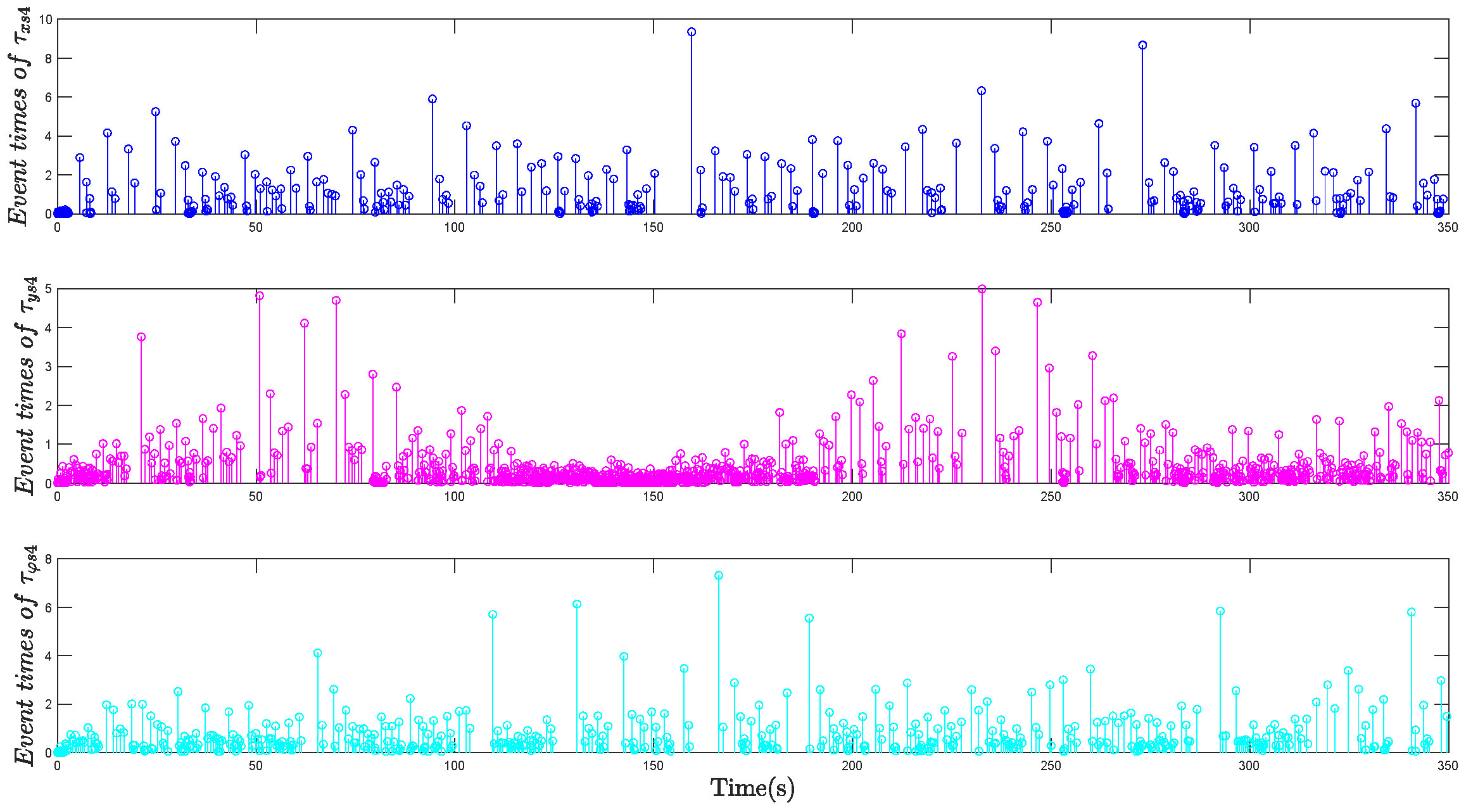
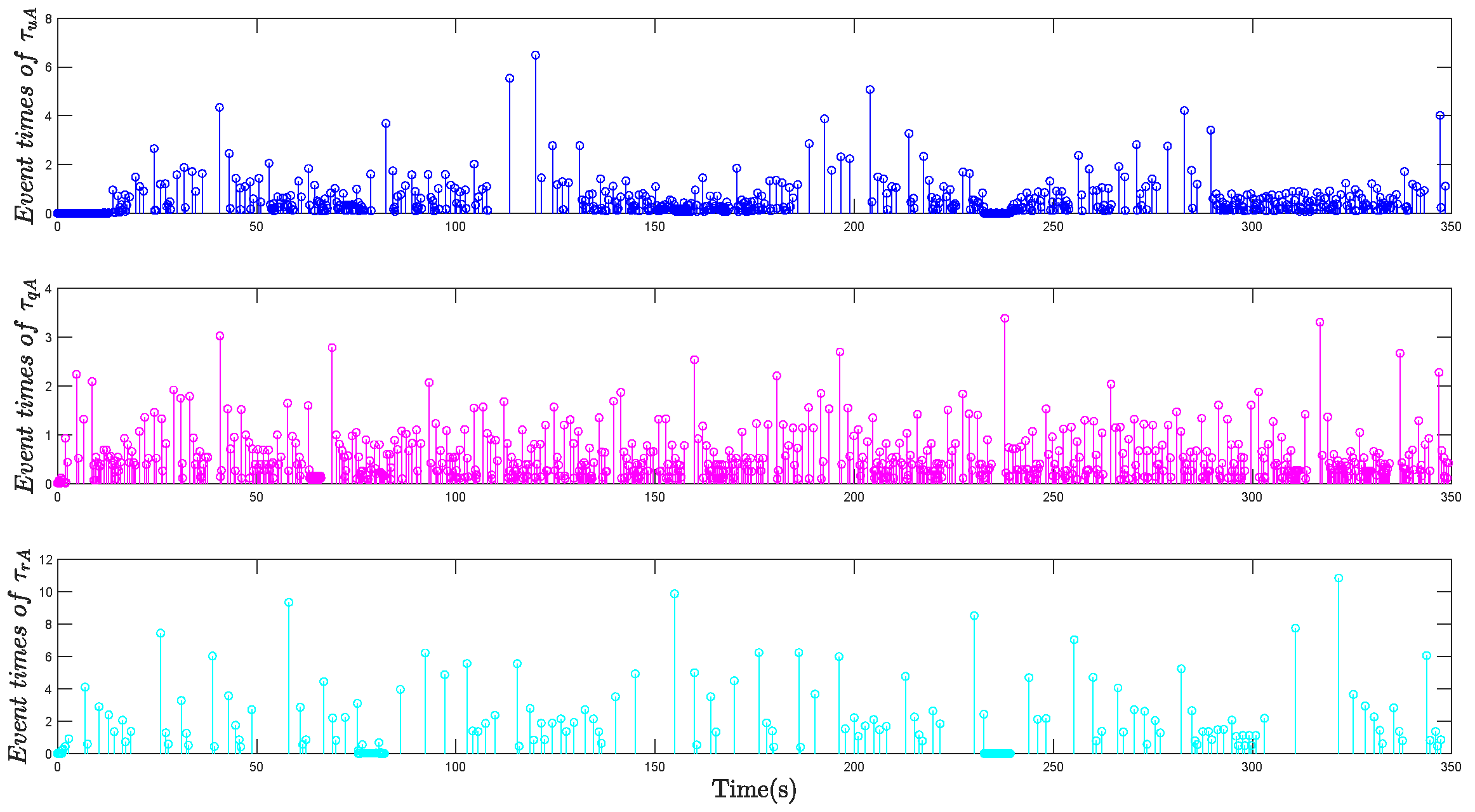
  • Different from the existing event-triggered mechanism [35], a memory event-triggered mechanism is proposed to better adapt to environmental changes according to historical data information, which can dramatically reduce the communication frequency and economize the communication resources.
  • A DRPSC strategy is constructed to improve the robustness and control precision in the presence of external disturbances and model uncertainty. Moreover, the heterogeneous underactuated AUV-USV system is guaranteed to be predefined-time stable.

2. Preliminaries and Problem Statement

2.1. Symbolic Declaration
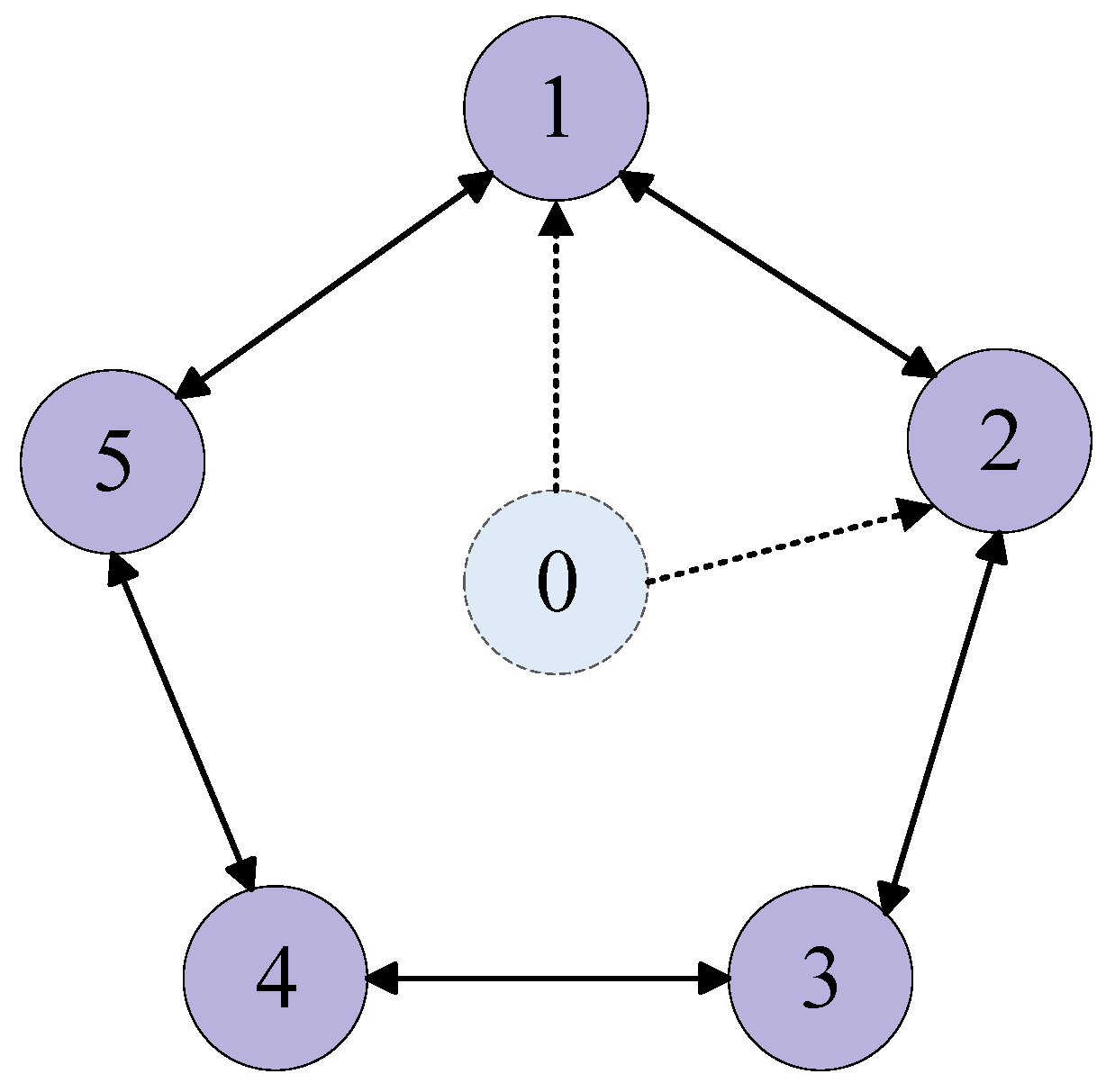
R N represent N dimensional Euclidean spaces; 1 N represents an N -dimensional unit column vector; Γ ( ) is the actual value; sgn ( ) represents the symbolic function; and d i a g ( ) is expressed as a diagonal matrix. represents the absolute value; is the matrix Euclidean norm; and represents the Kronecker product.

2.2. Graph Theory

The depiction encompasses the communication topology, whether directed or undirected, of N heterogeneous agents by Ξ = ( , ) T , where = υ 1 , υ 2 , , υ N denotes the node set. = ( υ i , υ j ) : υ i , υ j , i j × denotes the edge set, and a i j represents the information exchange between agent i and agent j . The adjacency matrix is expressed as A = [ a i j ] R ( N × N ) if there is an exchange of information between intelligence i and intelligence j and if ( υ i , υ j ) , a i j > 0 ; if not, a i j = 0 . N i = j ( i , j ) is the set of neighbors for the i th agent. If information is exchanged between agent i and the leader, then b i l = 1 ; if not, b i l = 0 . Then, the matrix B = d i a g ( b 1 l , b 2 l , , b N l ) . The weighted in-degree matrix D = d i a g d υ 1 , , d υ N + M and d υ i = j = 1 N a i j define the Laplacian matrix as L = D A .
Assumption 1.
In the directed or undirected spanning tree in  Ξ , the virtual leader serves as the root and ensures that at least one follower has the ability to obtain the leader’s information.
Remark 1.
In reference [37], Assumption 1 must be considered when solving the distributed trajectory tracking problem.

2.3. Relevant Lemmas

The following theorem is a stability theorem derived via Lyapunov and is used to analyze and prove the stability of nonlinear heterogeneous multi-agent systems in this study.
Lemma 1
([38,39]). Fixed-time stability of nonlinear systems:
Consider a nonlinear system
x ˙ ( t ) = F ( x ( t ) ) ,   x ( 0 ) = x 0
A continuous function existing in the radial direction is unbounded, V ( x ) : R n R , which can satisfy the following:
V ˙ ( x ) + a V p ( x ) + b V q ( x ) 0
with a > 0 , b > 0 , q > 1 , and 0 < p < 1 , the origin is fixed-time stable, and the settling time t s from any initial condition x 0 is bounded and satisfied:
t s 1 b ( q 1 ) + 1 a ( 1 p )
Lemma 2
([26]). Predefined-time stability of nonlinear systems:
A Lyapunov candidate function exists where V ( x ) : R n R + 0 is satisfied, and if and only if system (1) has predefined-time stability under initial conditions, the derivative of V ( x ) is as follows:
V ˙ ( x ) a 0 ι exp [ c 0 V ι ( x ) ] V 1 ι ( x ) + Δ
where a 0 > 0 , c 0 > 0 , 0 < ι 1 , and Δ R + . Therefore, the system (1) achieves predefined-time stability. For the predefined time T c and x ( t ) = 0 for all t T c , T c 1 a 0 c 0 Δ is satisfied.
Lemma 3
([40]). The matrices  H = L + B  and  P  are positive definite, and the eigenvalues of the  P  matrix are described as Equation (5). A positive definite matrix exists such that  Q = P H + H T P .
[ p 1 , p 2 , , p n ] T = H T 1 n P = d i a g p 1 , p 2 , , p n
Lemma 4
([41]). For arbitrary constants  ϖ > 0  and  l R , the following inequalities are satisfied:
0 ϖ ϖ tanh ( ϖ l ) 0.2785 l
Lemma 5
([42]). For a sequence of positive real values  y = ( y 1 , y 2 , , y n ) , then
( i = 1 n y i ) 1 n 1 n i = 1 n y i
Lemma 6
([42]). For groups of sequences  y = ( y 1 , y 2 , , y n )  and  z = ( z 1 , z 2 , , z n ) , if  y 1 y 2 y n  and  z 1 z 2 z n  or  y 1 y 2 y n  and  z 1 z 2 z n  are satisfied, then
i = 1 n y i z i 1 n i = 1 n y i i = 1 n z i

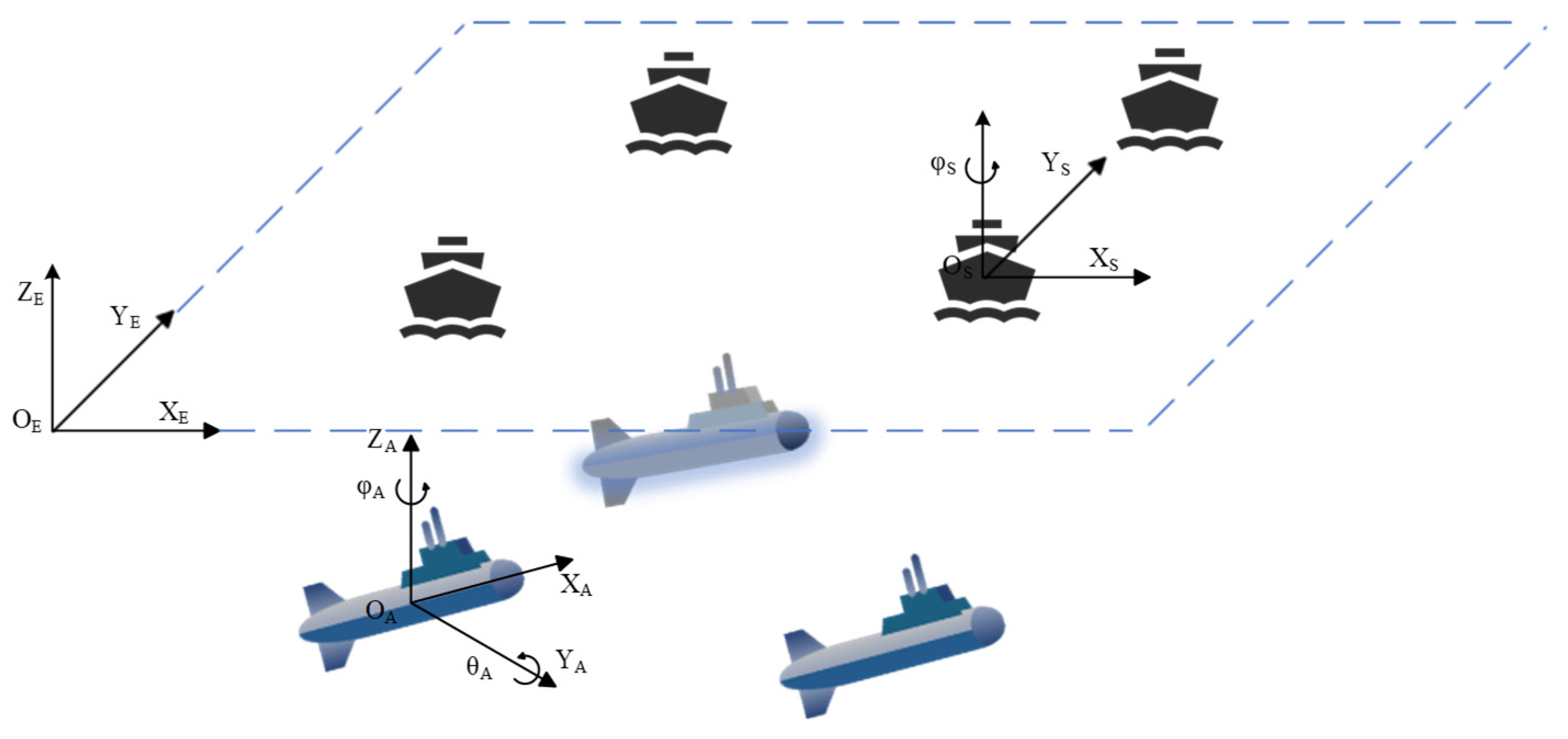
2.4. Problem Formulation

The surface and underwater heterogeneous multi-agent system consists of a virtual leader and some followers, where the followers include N USVs and M underactuated AUVs. To provide a detailed explanation of the formation trajectory tracking problem of an underactuated AUV-USV system in marine environments, Figure 1 visually presents an operation scenario diagram of the underactuated AUV-USV system. The agents above the horizontal plane are represented as four USVs, the two agents below the horizontal plane are represented as underactuated AUVs, and the agents with shadows at the edge are represented as virtual leaders.
Considering a marine heterogeneous multi-agent system with N USVs, the k th USV dynamics model is represented as [43]:
η s k = J ( η s k ) ν s k M k ν ˙ s k + C ( ν s k ) ν s k + D ( ν s k ) ν s k = Γ ( τ s k ) + f s k
where η s k = [ x s k , y s k , φ s k ] T represents the k th USV position variable and heading angle variable and where ν s k = [ u s k , v s k , r s k ] T represents the k th USV velocity variable and angular speed variable. Γ ( τ s k ) = [ Γ ( τ x s k ) , Γ ( τ y s k ) , Γ ( τ φ s k ) ] T represents the k th USV actual control input. M k R 3 N × 3 N represents the inertia matrix, C ( ν s k ) denotes the Coriolis and centripetal torque matrix, D ( ν s k ) denotes the damping matrix, J ( η s k ) is the rotation matrix, and f s k is the random disturbance in the marine environment.
Owing to the unpredictability of external environment disturbances, accurately obtaining the model parameters of USVs is difficult. To address the uncertainty of this model, we construct the following model matrix representation:
M k = M k + Δ M k C ( ν s k ) = C ( ν s k ) + Δ C ( ν s k ) D ( ν s k ) = D ( ν s k ) + Δ D ( ν s k )
where M k , C ( ν s k ) , and D ( ν s k ) are the nominal model matrices and where Δ M k , Δ C ( ν s k ) , and Δ D ( ν s k ) denote the matrices of unmodeled dynamics.
J ( η s k ) = cos φ s k   - sin φ s k     0 sin φ s k         cos φ s k         0           0                       0                       1 , M k = m 11       0             0 0           m 22       m 23 0           m 32       m 33 C ( ν s k ) = 0                 0                 c 13 , k 0                 0                 c 23 , k c 31 , k       c 32 , k           0 , D ( ν s k ) = d 11 , k         0               0 0             d 22 , k         d 23 , k 0             d 32 , k         d 33 , k
Defining χ s k , 1 = η s k and χ s k , 2 = η ˙ s k , the k th USV formula of the integrated dynamics model is as follows:
χ ˙ s k , 1 = χ s k , 2 χ ˙ s k , 2 = M ¯ k 1 Γ ( τ s k ) M ¯ k 1 [ C ¯ ( ν s k ) + D ¯ ( ν s k ) ] χ s k , 2 + M ¯ k 1 f ¯ s k
where M ¯ k = M k J ( η s k ) 1 , C ¯ ( ν s k ) = [ C ( ν s k ) M k J ( η s k ) 1 J ˙ ( η s k ) ] J ( η s k ) 1 , D ¯ ( ν s k ) = D ( ν s k ) J ( η s k ) 1 , and k = 1 , 2 , , N . f ¯ s k is the lumped uncertainty disturbance of the k th USV, including model uncertainty and unknown time-varying external environment disturbances, expressed as follows:
f ¯ s k = f s k Δ M k J ( η s k ) 1 η ¨ s k + [ Δ M k J ( η s k ) 1 J ˙ ( η s k ) Δ C ( ν s k ) Δ D ( ν s k ) ] J ( η s k ) 1 η ˙ s k
Considering the heterogeneous multi-agent system with M underactuated AUVs, the dynamic model of the m th underactuated AUV is as follows [44]:
x ˙ A m = u A m cos φ A m cos θ A m v A m sin φ A m + w A m sin θ A m cos φ A m y ˙ A m = u A m sin φ A m cos θ A m + v A m cos φ A m + w A m sin θ A m sin φ A m z ˙ A m = u A m sin θ A m + w A m cos θ A m θ ˙ A m = q A m φ ˙ A m = r A m / cos θ A m
u ˙ A m = 1 m 1 , A m Γ ( τ u A m ) + 1 m 1 , A m ( m 2 , A m v A m r A m m 3 , A m w A m q A m + f ¯ u , A m d 1 , A m u A m ) v ˙ A m = 1 m 2 , A m ( m 1 , A m u A m r A m + f ¯ v , A m d 2 , A m v A m ) w ˙ A m = 1 m 3 , A m ( m 1 , A m u A m q A m + f ¯ w , A m d 3 , A m w A m ) q ˙ A m = 1 m 5 , A m Γ ( τ q A m ) + 1 m 5 , A m ( ( m 3 , A m m 1 , A m ) u A m w A m G m + f ¯ q , A m d 5 , A m q A m ) r ˙ A m = 1 m 6 , A m Γ ( τ r A m ) + 1 m 6 , A m ( ( m 1 , A m m 2 , A m ) u A m v A m + f ¯ r , A m d 6 , A m r A m )
where m 1 , 2 , , M , η A m = [ x A m , y A m , z A m , θ A m , φ A m ] T , and ( x A m , y A m , z A m ) indicates the position of the m th underactuated AUV and where ( θ A m , φ A m ) indicates the pitch and yaw angles of the m th underactuated AUVs. ν A m = [ u A m , v A m , w A m , q A m , r A m ] denotes the corresponding speed (i.e., surge, sway, roll, pitch, and yaw speeds). d i , A m ( i = 1 , 2 , 3 , 5 , 6 ) represents the hydrodynamic coefficient, and m i , A m ( i = 1 , 2 , 3 , 5 , 6 ) represents the mass and inertia parameters of the m th search underactuated AUV. Γ ( τ ƛ A m ) and ( ƛ = u , q , r ) denote the actual control forces and moments of the m th search underactuated AUVs. G m = ρ g Δ G ¯ M ¯ L sin θ A m , where ρ , g , and Δ G ¯ M ¯ L denote the seawater density, gravitational acceleration, seawater discharge, and longitudinal center of the circle height, respectively, and where f ¯ n , A m ( n = u , v , w , q , r ) denotes the lumped uncertainty disturbances, including model uncertainties of underactuated AUVs and complex variable marine environmental disturbances, expressed as follows:
f ¯ u , A m = f u , A m m 1 , A m Δ m 1 , A m u ˙ A m + m 2 , A m Δ m 2 , A m v A m r A m m 3 , A m Δ m 3 , A m w A m q A m d 1 , A m Δ d 1 , A m u A m f ¯ v , A m = f v , A m m 2 , A m Δ m 2 , A m v ˙ A m m 1 , A m Δ m 1 , A m u A m r A m d 2 , A m Δ d 2 , A m v A m f ¯ w , A m = f w , A m m 3 , A m Δ m 3 , A m w ˙ A m m 1 , A m Δ m 1 , A m u A m q A m d 3 , A m Δ d 3 , A m w A m f ¯ q , A m = f q , A m m 5 , A m Δ m 5 , A m q ˙ A m + ( m 3 , A m Δ m 3 , A m m 1 , A m Δ m 1 , A m ) u A m w A m Δ G , m G m d 5 , A m Δ d 5 , A m q A m f ¯ r , A m = f r , A m m 6 , A m Δ m 6 , A m r ˙ A m + ( m 1 , A m Δ m 1 , A m m 2 , A m Δ m 2 , A m ) u A m r A m d 6 , A m Δ d 6 , A m r A m
where Δ m i , A m , Δ d i , A m , i = ( 1 , 2 , 3 , 5 , 6 ) , and Δ G , m denote the model uncertainty due to hydrodynamics and imprecise parameters, respectively, and where f n , A m R 5 × 1 and n = ( u , v , w , q , r ) denote unknown marine environmental time-varying disturbances.
Assumption 2.
The lumped uncertainty disturbances  f ¯ n , A m  and  f ¯ s k  of both the underactuated AUV and USV are asymptotically bounded, that is,  lim t 1 t 0 t f ¯ n , A m s d s f max  and  lim t 1 t 0 t f ¯ s k s d s f max . It is applicable not only to the case of unknown bounded disturbances but also to the cases of known and unbounded disturbances.
Owing to the physical performance limits of some power components, such as underactuated AUV and USV thrusters or the steering gear, when the control input value exceeds the physical limit, the actuator will enter the input saturation state, affecting the control stability performance. Therefore, some measures should be taken to limit the control input and ensure the operational stability of the underactuated AUV and USV. This function is expressed as follows:
Γ ( τ Z ) = L s , τ Z L s , τ Z , L d , < τ Z < L s , L d , τ Z L d
where Z = s k , ƛ A m , ƛ = u , q , r , k = 1 , , N , m = 1 , , M , and τ Z represent the desired control input and where L s and L d are denoted as the upper and lower bounds of the desired control input τ Z . We define the errors of τ Z and Γ ( τ Z ) as Δ τ Z = τ Z Γ ( τ Z ) .
The expression for the virtual leader’s dynamic equation is as follows:
χ ˙ L , 1 = χ L , 2 χ ˙ L , 2 = U L
where U L is bounded, χ L , 1 = [ x l , y l , z l , φ l ] T represents the position variable and angle variable information of the virtual leader, and χ L , 2 = [ u l , v l , w l , r l ] T represents the speed variable information for the virtual leader.
Assumption 3.
Assume that the state information variables  χ ˙ L , 1  and  χ ˙ L , 2  are bounded by the virtual leader.
The aim is to develop a formation tracking control strategy for Equations (9) and (14)’s underactuated AUV-USV systems under H control and a memory event-triggered mechanism that is stable for a predefined time.
  • In the underactuated AUV-USV system, all the error signals are bounded, the tracking error is limited to a certain small range near zero, and the system reaches stability at a predefined time.
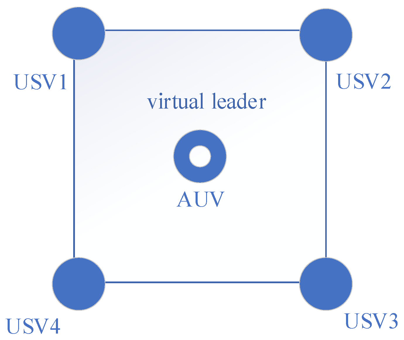
  • The underactuated AUV-USV system can complete the predetermined formation pattern within the predefined time and maintain the formation during subsequent control.
  • The effects of actuator input saturation, external environment disturbances, and model uncertainty in the underactuated AUV-USV system are eliminated.
  • The designed memory event-triggered mechanism does not exhibit “Zeno” behavior.

3. Main Results

Each agent has a design to monitor the state information through a distributed PTSO of the virtual leader. On the basis of the estimated information, a DRPSC is designed. Moreover, a PTADS was developed to mitigate the impact of input saturation in the actuator, and H control is used to address the marine external environment and model uncertainty. Through the design of a memory event-triggered mechanism, the communication frequency of the system is reduced, and resources are saved. Its convergence form is designed as the predefined time form by setting a small settling time T o b to ensure fast convergence of the observer and enhance the stability efficiency of the system.

3.1. Distributed Predefined-Time State Observer

According to Assumption 1, the state information is not all followers are well aware of the virtual leader. Hence, we create a distributed state observer that converges within a predefined time to estimate the state information of the virtual leader [45].
A distributed PTSO for each follower is designed as follows:
χ ^ ˙ L 1 , i = 1 ι o 1 T o b exp ( V ψ i , 1 ι o 1 ) V ψ i , 1 ι o 1 ψ i , 1 g 1 sgn ( ψ i , 1 ) χ ^ ˙ L 2 , i = 1 ι o 2 T o b exp ( V ψ i , 2 ι o 2 ) V ψ i , 2 ι o 2 ψ i , 2 g 2 sgn ( ψ i , 2 )
where ψ i , 1 = j = 1 N + M a i j ( χ ^ L 1 , i χ ^ L 1 , j ) + b i l ( χ ^ L 1 , i χ L , 1 ) , ψ i , 2 = j = 1 N + M a i j ( χ ^ L 2 , i χ ^ L 2 , j ) + b i l ( χ ^ L 2 , i χ L , 2 ) , i = 1 , , N + M indicates the i th agent, ι o 1 and ι o 2 are constant parameters and satisfy 0 < ι o 1 < 0.5 and 0 < ι o 2 < 0.5 , g 1 > 0 , and g 2 > 0 . χ ^ L 1 , i and χ ^ L 2 , i represent the i th agent’s position χ L , 1 and speed χ L , 2 estimate of the virtual leader, respectively. sgn ( x ) is a symbolic function expressed as sgn ( x ) : = 1 ,   i f   x < 0 0 ,   i f   x = 0 1 ,   i f   x > 0 . The state observation errors are assumed to be χ ˜ L 1 , i = χ ^ L 1 , i χ L , 1 and χ ˜ L 2 , i = χ ^ L 2 , i χ L , 2 . On the basis of models in Equation (18) and distributed observers in Equation (19), the following conclusions can be drawn:
χ ˜ ˙ L 1 , i = 1 ι o 1 T o b exp ( V ψ i , 1 ι o 1 ) V ψ i , 1 ι o 1 ψ i , 1 g 1 sgn ( ψ i , 1 ) χ L , 2 χ ˜ ˙ L 2 , i = 1 ι o 2 T o b exp ( V ψ i , 2 ι o 2 ) V ψ i , 2 ι o 2 ψ i , 2 g 2 sgn ( ψ i , 2 ) χ ˙ L , 2
Theorem 1.
For the estimated error (20), if  g 1 1 n χ L , 2  and  g 2 1 n χ ˙ L , 2  hold, the estimation errors  χ ˜ L 1 , i  and  χ ˜ L 2 , i  can settle to zero in  T o b .
Proof of Theorem 1.
First, we prove that lim t T o b χ ˜ L 1 , i = 0 . The candidate Lyapunov function is designed as follows:
V ψ i , 1 = 1 2 i = 1 N + M h = 1 p i ψ i h , 1 2
Matrix P is a positive definite diagonal matrix, p i in the above Equation (21) is the diagonal element, and h represents the h th dimension of each agent.
The derivative of Equation (21) yields the following:
V ˙ ψ i , 1 = i = 1 N + M h = 1 p i ψ i h , 1 ψ ˙ i h , 1 = i = 1 N + M h = 1 p i ψ i h , 1 ψ i h , 2
The following equation is defined in Equation (19):
i h , 1 = g 1 , i sgn ( ψ i h , 1 )
By substituting Equations (23) and (19) into Equation (22), we obtain
V ˙ ψ i , 1 = i = 1 N + M h = 1 p i ψ i h , 1 j = 1 N + M a i j i h , 1 j h , 1 + b i l i h , 1 χ L h , 2 i = 1 N + M h = 1 p i ψ i h , 1 1 2 ι o 1 T o b j = 1 N + M a i j exp ( V ψ i h , 1 ι o 1 ) V ψ i h , 1 ι o 1 ψ i h , 1 exp ( V ψ j h , 1 ι o 1 ) V ψ j h , 1 ι o 1 ψ j h , 1 + b i l exp ( V ψ i h , 1 ι o 1 ) V ψ i h , 1 ι o 1 ψ i h , 1
We define
Ψ i h , 1 = p i ψ i h , 1 j = 1 N + M a i j i h , 1 j h , 1 + b i l i h , 1 χ L h , 2
When ψ i h , 1 < 0 , we have i h , 1 χ L h , 2 0 , i h , 1 j h , 1 0 , and Ψ i h , 1 0 . When ψ i h , 1 > 0 , we have i h , 1 χ L h , 2 0 , i h , 1 j h , 1 0 , and Ψ i h , 1 0 . When ψ i h , 1 = 0 , we have Ψ i h , 1 = 0 .
Hence, from the above analysis, we can see that under certain conditions, Ψ i h , 1 0 always holds.
Then, Equation (24) is as follows:
V ˙ ψ i h , 1 p i ψ i h , 1 ι o 1 T o b i = 1 N + M h = 1 j = 1 N + M a i j exp ( V ψ i h , 1 ι o 1 ) V ψ i h , 1 ι o 1 ψ i , 1 exp ( V ψ j h , 1 ι o 1 ) V ψ j h , 1 ι o 1 ψ j , 1 + b i l exp ( V ψ i h , 1 ι o 1 ) V ψ i h , 1 ι o 1 ψ i h , 1 = 1 2 ι o 1 T o b exp ( V ψ i h , 1 ι o 1 ) V ψ i h , 1 ι o 1 ψ i h , 1 T Q I 4 ψ i h , 1 λ max ( P ) λ min ( Q ) 1 ι o 1 T o b exp ( V ψ i , 1 ι o 1 ) V ψ i , 1 1 ι o 1
where Equation (26), Q = P H + H T P , and, obviously, matrix Q is positive definite.
According to Theorem 1, we know that lim t T o b χ ˜ L 1 , i = 0 .
Second, we prove that lim t T o b χ ˜ L 2 , i = 0 , and the candidate Lyapunov function designed is as follows:
V ψ i , 2 = 1 2 i = 1 N + M h = 1 p i ψ i h , 2 2
Similar to proof lim t T o b χ ˜ L 1 , i = 0 , we can prove that lim t T o b χ ˜ L 2 , i = 0 .
Therefore, we can conclude that the observation errors χ ˜ L 1 , i and χ ˜ L 2 , i can settle to zero in T o b . □

3.2. Distributed Robust Predefined-Time Sliding Mode Control

The state information is obtained from the PTSO of the virtual leader in the previous section.

3.2.1. Predefined-Time Sliding Surface

The tracking errors for the k th follower USV are expressed as follows:
e s k , j = χ s k , j β s k , j χ ^ L j , s k
where j = 1 , 2 ; e s k , j = [ e x s k , j , e y s k , j , e φ s k , j ] T ; e s k , 1 is the position error; and e s k , 2 is the speed error of the k th USV, which satisfies e ˙ s k , 1 = e s k , 2 . We define χ ^ L j , s k = [ χ ^ L j , x s k , χ ^ L j , y s k , χ ^ L j , φ s k ] T , where χ ^ L j , s k represents the k th USV state estimate for the virtual leader in the previous section. We define β s k , j = [ β x s k , j , β y s k , j , β φ s k , j ] T as the boundary, which is the relative value held by the USV in position and angle to the virtual leader and meets β ˙ s k , 1 = β s k , 2 .
The tracking errors of the m th follower underactuated AUV are expressed as follows:
x e , A m = ( x A m β x A m x ^ L , A m ) cos θ A m cos φ A m ( z A m β z A m z ^ L , A m ) sin θ A m                     + ( y A m β y A m y ^ L , A m ) cos θ A m sin φ A m y e , A m = ( x A m β x A m x ^ L , A m ) sin φ A m + ( y A m β y A m y ^ L , A m ) cos φ A m z e , A m = ( x A m β x A m x ^ L , A m ) sin θ A m cos φ A m + ( z A m β z A m z ^ L , A m ) cos θ A m                     + ( y A m β y A m y ^ L , A m ) sin θ A m sin φ A m
In the above Equation (29), ^ L , A m ( = x , y , z ) is an estimate of the position state of the m th underactuated AUV for the virtual leader. β A m ( = x , y , z ) is the distance from the virtual leader, and β A m is defined as the boundary.
x ˙ e , A m = x ˙ ^ L , A m cos θ A m cos φ A m + u A m y ˙ ^ L , A m cos θ A m sin φ A m                     q A m z e , A m + z ˙ ^ L , A m sin θ A m + r A m y e , A m y ˙ e , A m = x ˙ ^ L , A m sin φ A m + v A m y ˙ ^ L , A m cos φ A m r A m ( x e , A m + z e , A m tan θ A m ) z ˙ e , A m = x ˙ ^ L , A m sin θ A m cos φ A m + r A m y e , A m tan θ A m y ˙ ^ L , A m sin θ A m sin φ A m                     z ˙ ^ L , A m cos θ A m + w A m + q A m x e , A m
where Equation (30) and ˙ ^ L , A m ( = x , y , z ) are an estimate of the speed state of the m th underactuated AUV for the virtual leader.
Three LOS errors (tracking position error ρ L , A m , pitch angle error θ L , A m , and yaw angle error φ L , A m ) are used to simplify the derivation of the underdriven AUV. The formula is expressed as follows:
ρ L , A m = x e , A m 2 + y e , A m 2 + z e , A m 2 θ L , A m = arctan 2 ( z e , A m , x e , A m 2 + y e , A m 2 ) φ L , A m = arctan 2 ( y e , A m , x e , A m )
By substituting Equation (31) into Equation (29), we obtain the following equation:
x e , A m = cos φ L , A m cos θ L , A m ρ L , A m y e , A m = sin φ L , A m cos θ L , A m ρ L , A m z e , A m = sin θ L , A m ρ L , A m
Taking the derivative of Equation (31) yields the following equation:
ρ ˙ L , A m = ζ ρ L 1 , A m + ζ ρ L 2 , A m + ζ ρ L , A m u A m θ ˙ L , A m = ζ θ L 1 , A m + ζ θ L 2 , A m + ζ θ L , A m q A m φ ˙ L , A m = ζ φ L 1 , A m + ζ φ L 2 , A m + ζ φ L , A m r A m
where
ζ ρ L , A m = cos ( θ L , A m ) cos ( φ L , A m ) ζ ρ L 1 , A m = v A m cos ( θ L , A m ) sin ( φ L , A m ) + w A m sin ( θ L , A m ) ζ ρ L 2 , A m = ζ 1 d , A m cos ( θ L , A m ) cos ( φ L , A m ) + ζ 2 d , A m cos ( θ L , A m ) sin ( φ L , A m ) + ζ 3 d , A m sin ( θ L , A m ) ζ θ L , A m = cos ( φ L , A m ) ζ θ L 1 , A m = r A m tan ( θ A m ) sin ( φ L , A m ) ζ θ L 2 , A m = cos ( θ L , A m ) ( w A m + ζ 3 d , A m ) / ρ L , A m sin ( θ L , A m ) cos ( φ L , A m ) ( u A m + ζ 1 d , A m ) / ρ L , A m                         sin ( θ L , A m ) sin ( φ L , A m ) ( v A m + ζ 2 d , A m ) / ρ L , A m ζ φ L , A m = ( 1 + tan ( θ A m ) tan ( θ L , A m ) cos ( φ L , A m ) ) ζ φ L 1 , A m = q A m tan ( θ L , A m ) sin ( φ L , A m ) ζ φ L 2 , A m = ( u A m + ζ 1 d , A m ) sin ( φ L , A m ) ρ L , A m cos ( θ L , A m ) + ( v A m + ζ 2 d , A m ) cos ( φ L , A m ) ρ L , A m cos ( θ L , A m ) ζ 1 d , A m = x ˙ ^ L , A m cos ( θ A m ) cos ( φ A m ) y ˙ ^ L , A m cos ( θ A m ) sin ( φ A m ) + z ˙ ^ L , A m sin ( θ A m ) ζ 2 d , A m = x ˙ ^ L , A m sin ( φ A m ) y ˙ ^ L , A m cos ( φ A m ) ζ 3 d , A m = x ˙ ^ L , A m sin ( θ A m ) cos ( φ A m ) y ˙ ^ L , A m sin ( θ A m ) sin ( φ A m ) z ˙ ^ L , A m cos ( θ A m )
The derivative equation of Equation (33) is as follows:
ρ ¨ L , A m = ζ ρ L , A m u ˙ A m + ζ ρ d , A m + ζ ˙ ρ L 1 , A m + ζ ˙ ρ L 2 , A m θ ¨ L , A m = ζ θ L , A m q ˙ A m + ζ θ d , A m + ζ ˙ θ L 1 , A m + ζ ˙ θ L 2 , A m φ ¨ e L , A m = ζ φ L , A m r ˙ A m + ζ φ d , A m + ζ ˙ φ L 1 , A m + ζ ˙ φ L 2 , A m
where
ζ ρ d , A m = u A m ( sin ( θ L , A m ) cos ( φ L , A m ) θ ˙ L , A m + cos ( θ L , A m ) sin ( φ L , A m ) φ ˙ L , A m ) ζ θ d , A m = q A m sin ( φ L , A m ) φ ˙ L , A m ζ φ L , A m = r A m ( θ ˙ A m tan ( θ L , A m ) cos ( φ L , A m ) cos 2 ( θ A m ) + tan ( θ A m ) θ ˙ L , A m cos ( φ L , A m ) cos 2 ( θ L , A m )                         tan ( θ A m ) tan ( θ L , A m ) sin ( φ L , A m ) φ ˙ L , A m )
A predefined-time sliding mode surface is designed:
s s k = e s k , 2 + k s k e s k , 1 + 1 2 ι 1 , s k T s exp ( V e s k , 1 ι 1 , s k ) V e s k , 1 ι 1 , s k e s k , 1 s A m = ˙ A m + k A m A m + 1 2 ι 1 , A m T s exp ( V A m ι 1 , A m ) V A m ι 1 , A m A m
where A m = ρ L , A m , θ L , A m , φ L , A m , ˙ A m = ρ ˙ L , A m , θ ˙ L , A m , φ ˙ L , A m , 0 < ι 1 , s k < 0.5 , 0 < ι 1 , A m < 0.5 , and k s k > 0 and k A m > 0 are constants, and where T s indicates the user-defined time.
Taking the derivative of Equation (35), it can be obtained that
s ˙ s k = e ˙ s k , 2 + k s k e s k , 2 + E s k s ˙ A m = ¨ A m + k A m ˙ A m + E A m
where ¨ A m = ρ ¨ L , A m , θ ¨ L , A m , φ ¨ L , A m and
E s k = 1 2 ι 1 , s k T s exp ( V e s k , 1 ι 1 , s k ) V e s k , 1 ι 1 , s k e s k , 2 + 1 2 T s exp ( V e s k , 1 ι 1 , s k ) V e s k , 1 1 V e s k , 1 1 ι 1 , s k e s k , 1 T e s k , 2 e s k , 1 E A m = 1 2 ι 1 , A m T s exp ( V A m ι 1 , A m ) V A m ι 1 , A m ˙ A m + 1 2 T s exp ( V A m ι 1 , A m ) ( V A m 1 V A m 1 ι 1 , A m ) A m 2 ˙ A m
where V e s k , 1 = 1 2 e s k , 1 T e s k , 1 and V A m = 1 2 A m 2 .
Considering Equations (12), (15), and (36) together, the controller can be designed as
τ s k = M ¯ k ( χ ˙ ^ L 2 , s k k s k e s k , 2 E s k ) k 1 , s k s s k 1 2 ι 2 , s k T c exp ( V s s k ι 2 , s k ) V s s k ι 2 , s k s s k                     + Δ τ s k f ¯ s k + C ¯ ( ν s k ) χ s k , 2 + D ¯ ( ν s k ) χ s k , 2 τ ƛ A m = A ƛ A m 1 ( ζ d , A m + ζ ˙ 1 , A m + ζ ˙ 2 , A m + k A m ˙ A m + E A m                     + k 1 , A m s A m + 1 2 ι 2 , A m T c exp ( V s A m ι 2 , A m ) V s A m ι 2 , A m s A m ) + Δ τ ƛ A m f ¯ ƛ , A m B ƛ A m
where τ s k and τ ƛ A m represent the control rates, k = 1 , , N , m = 1 , , M , ƛ = u , q , r , and 0 < ι 2 , s k < 0.5 , and where 0 < ι 2 , A m < 0.5 , V s s k = 1 2 s s k T s s k , and V s A m = 1 2 s A m 2 ; here
A u A m = ζ ρ L , A m m 1 , A m , A q A m = ζ θ L , A m m 5 , A m , A r a m = ζ φ L , A m m 6 , A m B u A m = m 2 , A m v A m r A m m 3 , A m w A m q A m d 1 , A m u A m B q A m = ( m 3 , A m m 1 , A m ) u A m w A m G m d 5 , A m q A m B r A m = ( m 1 , A m m 2 , A m ) u A m v A m d 6 , A m r A m

3.2.2. Predefined-Time Auxiliary Dynamic System and Predefined-Time H Control

Owing to the phenomenon of actuator input saturation in the underactuated AUV-USV system, when the command signal of the control algorithm exceeds the physical limit value of the actuator components, such as the USV or the propeller of the underactuated AUV, the stability and maneuverability of the underactuated AUV-USV system are affected. To relieve the impact of actuator input saturation on the underactuated AUV-USV system, a predefined-time auxiliary dynamic system for the heterogeneous multi-agent system in marine areas is designed to improve the stability and controllability of the AUV-USV system. The formula is as follows:
χ ˙ c , s k = k c , s k s s k i = 1 3 s i s k Δ τ i s k χ c , s k 2 χ c , s k 1 2 ι 2 , s k T c exp ( V χ c , s k ι 2 , s k ) V χ c , s k ι 2 , s k χ c , s k , χ c , s k σ s k k c , s k s s k 1 2 ι 2 , s k T c exp ( V χ c , s k ι 2 , s k ) V χ c , s k ι 2 , s k χ c , s k , χ c , s k < σ s k χ ˙ c , A m = k c , A m s A m s A m A ƛ A m Δ τ ƛ A m χ c , A m 2 χ c , A m 1 2 ι 2 , A m T c exp ( V χ c , A m ι 2 , A m ) V χ c , A m ι 2 , A m χ c , A m , χ c , A m σ A m k c , A m s A m 1 2 ι 2 , A m T c exp ( V χ c , A m ι 2 , A m ) V χ c , A m ι 2 , A m χ c , A m , χ c , A m < σ A m
where Δ τ s k = [ Δ τ x s k , Δ τ y s k , Δ τ φ s k ] T , χ c , s k = [ χ c , x s k , χ c , y s k , χ c , φ s k ] T , V c , s k = 1 2 χ c , s k T χ c , s k , and V c , A m = 1 2 χ c , A m 2 ; σ s k and σ A m are positively designed parameters; k c , s k > 0 and k c , A m > 0 are constants; and T c is user-defined.
Remark 2.
In Equation (38), to avoid singularities,  σ s k  and  σ A m  are small positive constants and close to zero. To maintain the proper functioning of the PTADS, the initial states of  χ c , s k  and  χ c , A m  satisfy  χ c , s k ( 0 ) σ s k  and  χ c , A m ( 0 ) σ A m .
Given the underactuated AUV-USV system model uncertainty and the external disturbances, we use H control theory to solve these problems.
Definition 1
([46]). For the following error dynamic systems,
x ˙ = f ( t ) + ( x ) u ¯ + Φ ( x ) Κ = ϕ ( x )
where  x  is the state vector of the error system,  u ¯  represents the control input,  Κ  is the performance vector,  f ( t )  represents the uncertain disturbances, and  ( x )  and  Φ ( x )  represent the system functions.
Define  ϒ > 0  if, for  f L 2 [ t 0 , t 1 ] ,  t 1 > t 0 . We can obtain the following:
t 0 t 1 Κ ( t ) 2 d t ϒ 2 t 0 t 1 f ( t ) 2 d t
then the L2 gain of the error dynamic systems is less than or equal to  ϒ .
For system (39), assume that a Lyapunov function  V ( x )  exists in the origin domain  U ^ 0 R n . If the controller can ensure that the system satisfies the elements of Lemma 2 and the following two conditions, then the controller may be called a predefined-time H controller.
  • V ( x )  is positive definite in  U ^ 0 .
  • V ˙ ( t ) + a 0 b 0 exp [ c 0 V ι ( x ) ] V 1 ι ( x ) 1 2 ( ϒ 2 f 2 Κ 2 ) + Δ .
Therefore, system (39) is a locally predefined time, and the system gain is less than or equal to  ϒ .
Proof. 
If V ( x ) > 0 , f ( t ) = 0 , in condition (2) above, this formula is written as follows:
V ˙ ( t ) + a 0 b 0 exp [ c 0 V ι ( x ) ] V 1 ι ( x ) 1 2 Κ 2 + Δ 0
According to Lemma 2, system (39) is stable at the predefined time.
If V ( x ) > 0 , f ( t ) 0 , in condition (2) above, this equation is written as follows:
V ˙ ( t ) + a 0 b 0 exp [ c 0 V ι ( x ) ] V 1 ι ( x ) 1 2 ( ϒ 2 f 2 Κ 2 ) + Δ
From Equation (40), the L2 gain of system (39) is less than or equal to ϒ . Therefore, system (39) is predefined for time stability, and the system gain is less than or equal to ϒ . □
According to Equation (36), the error variable is defined as follows:
s ˙ s k = M ¯ k 1 ( τ s k Δ τ s k + f ¯ s k C ¯ ( ν s k ) χ s k , 2 D ¯ ( ν s k ) χ s k , 2 ) χ ˙ ^ L 2 , s k + k s k e s k , 2 + E s k s ˙ A m = A ƛ A m ( τ ƛ A m Δ τ ƛ A m + B ƛ A m + f ¯ ƛ , A m ) + ζ d , A m + ζ ˙ 1 , A m + ζ ˙ 2 , A m + k A m ˙ A m + E A m
where ƛ = u , q , r , k = 1 , , N , and m = 1 , , M , and the system performance vector is selected as follows:
Κ s k = s k s s k , Κ A m = A m s A m
The DRPSC strategy of the heterogeneous multi-agent system combining the auxiliary dynamic system and H control can be redesigned as follows:
τ s k = M ¯ k ( χ ˙ ^ L 2 , s k k s k e s k , 2 E s k ) k 1 , s k s s k 1 2 ι 2 , s k T c exp ( V s s k ι 2 , s k ) V s s k ι 2 , s k s s k                     + C ¯ ( ν s k ) χ s k , 2 + D ¯ ( ν s k ) χ s k , 2 + ( s s k T ) 1 χ c , s k T k c , s k s s k ( 1 2 ϒ s k 2 + s k 2 2 ) s s k τ ƛ A m = - B ƛ A m A ƛ A m 1 ( ζ d , A m + ζ ˙ 1 , A m + ζ ˙ 2 , A m + k A m ˙ A m + E A m + k 1 , A m s A m                     + 1 2 ι 2 , A m T c exp ( V s A m ι 2 , A m ) V s A m ι 2 , A m s A m k c , A m χ c , A m + ( 1 2 ϒ A m 2 + A m 2 2 ) s A m )
where τ s k and τ ƛ A m represent the final control rates, k = 1 , , N , m = 1 , , M , and ƛ = u , q , r . In Algorithm 1, the control flowchart of the proposed control algorithm DRPSC is presented.
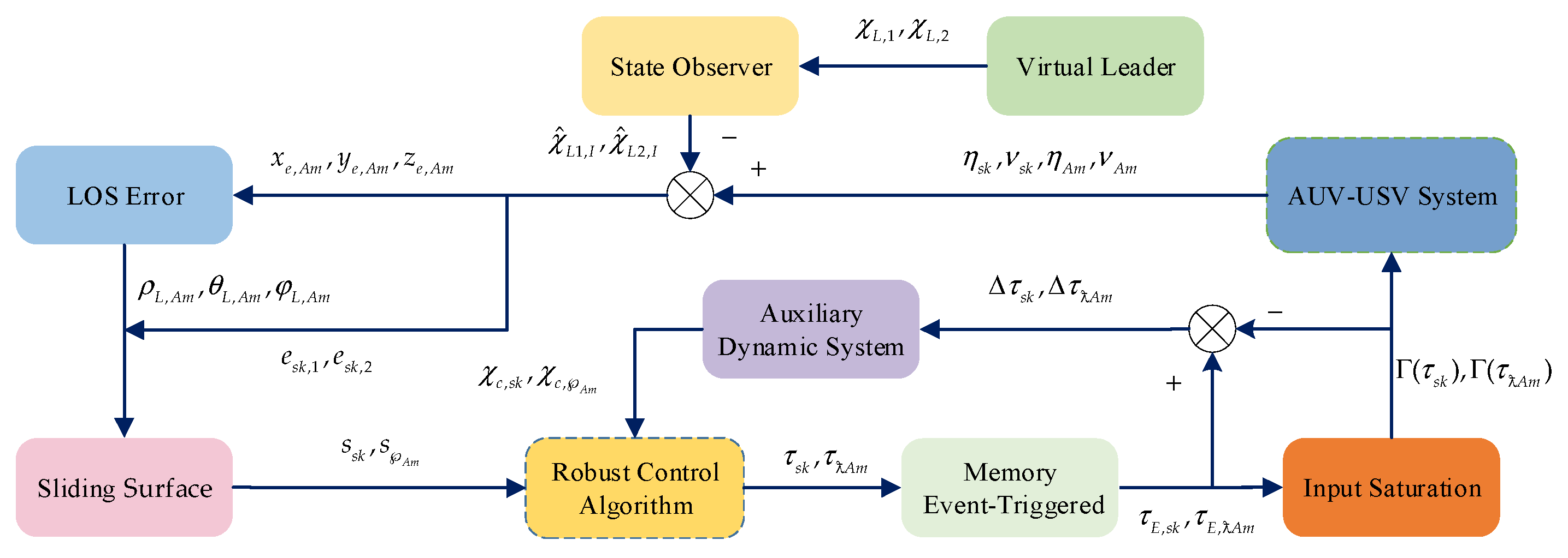
  Algorithm 1 The distributed robust predefined-time sliding mode control algorithm.
      Step I: Initialization: Define the state space model of the AUV-USV heterogeneous multi-agent system, (9) and (14).
      Step II: Define the formation tracking error, (28) and (29), and perform LOS error conversion for the five-degree-of-freedom underdriven AUV (31).
      Step III: Design a distributed predefined-time state observer, (19), to obtain the state information of the virtual leader.
      Step IV: Define the predefined-time sliding surface, (35).
      Step V: Design a predefined-time auxiliary dynamic system to solve the problem of actuator input saturation, (38), combined with H control for the system and lumped uncertainty disturbance.
      Step VI: Design the final controller, (45).
      Step VII: Design the memory event-triggered mechanism, (46) and (47).
Stop Algorithm

3.2.3. Memory Event-Triggered Mechanism

To reduce the controller’s communication frequency and minimize the wastage of communication resources, combined with the distributed predefined-time controller proposed above, a distributed predefined-time formation controller triggered by events based on memory is designed. The expression is as follows:
τ ¯ s k = ( 1 + ξ 1 , s k κ 1 , s k ) τ s k tanh ( s s k T τ s k l s k ) + 1 3 Θ 2 , s k ξ 2 , s k + Θ 1 , s k ξ 1 , s k κ 2 , s k τ E , s k ( t Λ ) τ ¯ ƛ A m = ( 1 + ξ 1 , ƛ A m κ 1 , A m ) τ ƛ A m tanh ( s A m A ƛ A m τ ƛ A m l ƛ A m ) + Θ 2 , A m ξ 2 , A m + Θ 1 , A m ξ 1 , A m κ 2 , A m τ E , A m ( t Λ )
where Θ 1 , s k , Θ 2 , s k , Θ 1 , A m , and Θ 2 , A m are the variables that satisfy Θ 1 , s k < 1 , Θ 2 , s k < 1 , Θ 1 , A m < 1 , and Θ 2 , A m < 1 . The triggering conditions of the memory event-triggered mechanism are defined as follows:
τ E , s k ( t ) = τ ¯ s k ( t k ) , τ E , ƛ A m ( t ) = τ ¯ ƛ A m ( t k )                 t [ t k , t k + 1 ) t k + 1 = inf t R | e E , Z ( t ) ξ 1 , Z ( κ 1 , Z τ E , Z ( t ) + κ 2 , Z τ E , Z ( t Λ ) ) + 1 Z ξ 2 , Z κ 2 , Z = ξ 3 , Z e ξ 4 , Z τ E , Z ( t Λ ) τ E , Z ( t ) τ E , Z ( t ) κ 1 , Z = 1 κ 2 , Z
where Z = s k , ƛ A m ; ƛ = u , q , r ; k = 1 , , N ; m = 1 , , M ; ξ 1 , Z , ξ 2 , Z , ξ 3 , Z , ξ 4 , Z , l Z are positive constants; and Λ is the time constant. The error of the memory event-triggered mechanism is defined as e E , Z ( t ) = τ ¯ Z ( t ) τ E , Z ( t ) .
Remark 3.
If  t k [ t k , t k + 1 ) ,  τ E , s k ( t )  and  τ E , ƛ A m ( t )  equal  τ ¯ s k ( t k )  and  τ ¯ ƛ A m ( t k ) . When the trigger conditions (47) hold, the control inputs  τ ¯ s k ( t k )  and  τ ¯ ƛ A m ( t k )  are updated to  τ E , s k ( t )  and  τ E , ƛ A m ( t ) .
Remark 4.
The memory event-triggered mechanism is different from the ordinary triggering mechanism. The historical information stored in the memory can improve the response speed and flexibility of the system by changing the triggering conditions, and it can also save resources better.
The control framework of the proposed DRPSC methodology is shown in Figure 2.
Remark 5.
The DRPSC strategy shown in Figure 2 is based on the following modular design: PTSO, PTAD, METM, SMC, and H control. These methods are applicable to scenarios that require state estimation, have control input limitations, need to optimize communication resources, and handle external disturbances and model uncertainties. These modular components can be combined and adjusted according to different application requirements, thereby achieving greater versatility. For example, for systems with higher dynamic characteristics, the parameters of sliding mode control can be adjusted, or more complex robust control strategies can be introduced.
Remark 6.
Although the DRPSC strategy proposed in this paper is designed for AUV-USV formation missions, the control strategy is also applicable to other heterogeneous multi-agent systems, such as the cooperative tasks of unmanned aerial vehicles (UAVs) and unmanned ground vehicles (UGVs) in air–ground heterogeneous multi-agent systems; the cooperative tasks of UAVs and USVs in air–water heterogeneous multi-agent systems; and the cooperative tasks of different types of UGVs in ground–ground heterogeneous multi-agent systems. However, different types of agents (such as AUVs, USVs, UAVs, and UGVs) have different dynamic characteristics and may be equipped with different sensors and actuators, and the design of observers and control inputs needs to be adjusted. Moreover, different types of agents may use different communication protocols, and the compatibility of communication mechanisms needs to be ensured.

4. Stability Analysis

Theorem 2.
When  s s k = 0  and  s A m = 0  are satisfied, the position errors  e s k , 1  and  A m  of the formation trajectory tracking can settle within the zero region within the predefined time  T o b + T s .
Proof of Theorem 2.
When s s k = 0 and s A m = 0 , we can construct a candidate Lyapunov function:
V e s k , 1 = 1 2 e s k , 1 T e s k , 1 , V A m = 1 2 A m 2
Taking the derivative of V e Z , 1 and V A m by Equation (48), it can be obtained that
V ˙ e s k , 1 = e s k , 1 T e s k , 2                 = k s k e s k , 1 T e s k , 1 1 2 ι 1 , s k T s exp ( V e s k , 1 ι 1 , s k ) V e s k , 1 ι 1 , s k e s k , 1 T e s k , 1                 1 ι 1 , s k T s exp ( V e s k , 1 ι 1 , s k ) V e s k , 1 1 ι 1 , s k V ˙ A m = A m ˙ A m                 = k A m A m 2 1 2 ι 1 , A m T s exp ( V A m ι 1 , A m ) V A m ι 1 , A m A m 2                 1 ι 1 , A m T s exp ( V A m ι 1 , A m ) V A m 1 ι 1 , A m
According to the above Equation (49) and Lemma 2, when s s k = 0 and s A m = 0 , the tracking errors e s k , 1 and A m of the underactuated AUV and USV converge to zero in T o b + T s . □
Theorem 3.
Considering the underactuated AUV-USV heterogeneous multi-agent system (9) and (14)–(15), on the basis of the auxiliary dynamic system (38), the sliding mode surface (35), memory event-triggered mechanism, and H control,  s s k ,  s A m ,  χ c , s k , and  χ c , A m  can converge to zero within  T o b + T s + T c .
Proof of Theorem 3.
According to (47), we can obtain
τ ¯ Z ( t ) = ( 1 + Θ 1 , Z ξ 1 , Z κ 1 , Z ) τ E , Z ( t ) + Θ 1 , Z ξ 1 , Z κ 2 , Z τ E , Z ( t Λ ) + 1 Z Θ 2 , Z ξ 2 , Z
The above formula can be converted to obtain the following:
τ E , Z ( t ) = τ ¯ Z ( t ) 1 Z Θ 2 , Z ξ 2 , Z Θ 1 , Z ξ 1 , Z κ 2 , Z τ E , Z ( t Λ ) 1 + Θ 1 , Z ξ 1 , Z κ 1 , Z
Considering a candidate Lyapunov function,
V M s k = 1 2 s s k T M ¯ k s s k + 1 2 χ c , s k T χ c , s k V M A m = 1 2 s A m 2 + 1 2 χ c , A m 2
Taking the derivative of the above Equation (52) and proving that the system gain L2 satisfies L 2 ϒ Z , the following design is used:
V ˙ M s k = s s k T M ¯ k s ˙ s k + χ c , s k T χ ˙ c , s k + 1 2 ( s k s s k 2 ϒ s k 2 f ¯ s k 2 ) V ˙ M A m = s A m T s ˙ A m + χ c , A m T χ ˙ c , A m + 1 2 ( A m s A m 2 ϒ A m 2 A ƛ A m f ¯ ƛ , A m 2 )
  • χ c , s k σ s k and χ c , A m σ A m
Putting Equations (36) and (38) into (53), we can obtain
V ˙ M s k = s s k T M ¯ k ( χ ˙ s k , 2 χ ˙ ^ L 2 , s k + k s k e s k , 2 + E s k ) + 1 2 ( s k s s k 2 ϒ s k 2 f ¯ s k 2 )                   + χ c , s k T ( k c , s k s s k i = 1 3 s i s k Δ τ i s k χ c , s k 2 χ c , s k 1 2 ι 2 , s k T c exp ( V χ c , s k ι 2 , s k ) V χ c , s k ι 2 , s k χ c , s k ) V ˙ M A m = s A m ( ¨ A m + k A m ˙ A m + E A m ) + 1 2 ( A m s A m 2 ϒ A m 2 A ƛ A m f ¯ ƛ , A m 2 )                   + χ c , A m ( k c , A m s A m s A m A ƛ A m Δ τ ƛ A m χ c , A m 2 χ c , A m 1 2 ι 2 , A m T c exp ( V χ c , A m ι 2 ) V χ c , A m ι 2 χ c , A m )
By substituting Equations (12), (15), and (34) into Formula (54), we obtain
V ˙ M s k = s s k T [ Γ ( τ E , s k ) ( C ¯ ( ν s k ) + D ¯ ( ν s k ) ) χ s k , 2 + f ¯ s k ]                     + s s k T M ¯ k ( χ ˙ ^ L 2 , s k + k s k e s k , 2 + E s k ) + 1 2 ( s k s s k 2 ϒ s k 2 f ¯ s k 2 )                     k c , s k χ c , s k T s s k i = 1 3 s i s k Δ τ i s k χ c , s k 2 χ c , s k T χ c , s k χ c , s k T 1 2 ι 2 , s k T c exp ( V χ c , s k ι 2 , s k ) V χ c , s k ι 2 , s k χ c , s k V ˙ M A m = s A m [ A ƛ A m ( Γ ( τ E , ƛ A m ) + B ƛ A m + f ¯ ƛ , A m ) + ζ d , A m + ζ ˙ 1 , A m + ζ ˙ 2 , A m + k A m ˙ A m + E A m ]                         + 1 2 ( A m s A m 2 ϒ A m 2 A ƛ A m f ¯ ƛ , A m 2 ) χ c , A m k c , A m s A m                       χ c , A m s A m A ƛ A m Δ τ ƛ A m χ c , A m 2 χ c , A m χ c , A m 1 2 ι 2 , A m T c exp ( V χ c , A m ι 2 , A m ) V χ c , A m ι 2 , A m χ c , A m
By substituting Equations (17) and (51) into (55), we obtain
V ˙ M s k = s s k T [ τ ¯ s k ( t ) 1 s k Θ 2 , s k ξ 2 , s k Θ 1 , s k ξ 1 , s k κ 2 , s k τ E , s k ( t Λ ) 1 + Θ 1 , s k ξ 1 , s k κ 1 , s k ]                     + s s k T [ Δ τ s k ( C ¯ ( ν s k ) + D ¯ ( ν s k ) ) χ s k , 2 + f ¯ s k ]                     + s s k T M ¯ k ( χ ˙ ^ L 2 , s k + k s k e s k , 2 + E s k ) + 1 2 ( s k s s k 2 ϒ s k 2 f ¯ s k 2 )                     k c , s k χ c , s k T s s k i = 1 3 s s k , i Δ τ s k , i 1 ι 2 , s k T c exp ( V χ c , s k ι 2 , s k ) V χ c , s k 1 ι 2 , s k V ˙ M A m = s A m [ A ƛ A m τ ¯ ƛ A m ( t ) Θ 2 , A m ξ 2 , A m Θ 1 , A m ξ 1 , A m κ 2 , A m τ E , ƛ A m ( t Λ ) 1 + Θ 1 , A m ξ 1 , A m κ 1 , A m ]                         + 1 2 ( A m s A m 2 ϒ A m 2 A ƛ A m f ¯ ƛ , A m 2 )                         + s A m [ A ƛ A m ( Δ τ ƛ A m + B ƛ A m + f ¯ ƛ , A m ) + ζ d , A m + ζ ˙ 1 , A m + ζ ˙ 2 , A m + k A m ˙ A m + E A m ]                         χ c , A m k c , A m s A m s A m A ƛ A m Δ τ ƛ A m 1 ι 2 , A m T c exp ( V χ c , A m ι 2 , A m ) V χ c , A m 1 ι 2 , A m
According to Lemma 4, the following inequality can be derived:
s s k T [ τ ¯ s k ( t ) 1 s k Θ 2 , s k ξ 2 , s k Θ 1 , s k ξ 1 , s k κ 2 , s k τ E , s k ( t Λ ) ] 1 + Θ 1 , s k ξ 1 , s k κ 1 , s k s s k T [ τ ¯ s k ( t ) 1 s k Θ 2 , s k ξ 2 , s k Θ 1 , s k ξ 1 , s k κ 2 , s k τ E , s k ( t Λ ) ] 1 + ξ 1 , s k κ 1 , s k s A m A ƛ A m [ τ ¯ ƛ A m ( t ) Θ 2 , A m ξ 2 , A m Θ 1 , A m ξ 1 , A m κ 2 , A m τ E , ƛ A m ( t Λ ) ] 1 + Θ 1 , A m ξ 1 , A m κ 1 , A m s A m A ƛ A m [ τ ¯ ƛ A m ( t ) Θ 2 , A m ξ 2 , A m Θ 1 , A m ξ 1 , A m κ 2 , A m τ E , ƛ A m ( t Λ ) ] 1 + ξ 1 , A m κ 1 , A m ϖ ϖ tanh ( ϖ l ) 0.2785 l ϖ
Bringing the predefined-time controllers (46) and (57) into (56), we obtain
V ˙ M s k s s k T τ s k + s s k T [ Δ τ s k ( C ¯ ( v s k ) + D ¯ ( v s k ) ) χ s k , 2 + f ¯ s k ]                     + s s k T M ¯ k ( χ ˙ ^ L 2 , s k + k s k e s k , 2 + E s k ) + 1 2 ( s k s s k 2 ϒ s k 2 f ¯ s k 2 )                     k c , s k χ c , s k T s s k i = 1 3 s i s k Δ τ i s k 1 ι 2 , s k T c exp ( V χ c , s k ι 2 , s k ) V χ c , s k 1 ι 2 , s k + 0.557 l V ˙ M A m s A m A ƛ A m τ ƛ A m + 1 2 ( A m s A m 2 ϒ A m 2 A ƛ A m f ¯ ƛ , A m 2 )                         + s A m [ A ƛ A m ( Δ τ ƛ A m + B ƛ A m + f ¯ ƛ , A m ) + ζ d , A m + ζ ˙ 1 , A m + ζ ˙ 2 , A m + k A m ˙ A m + E A m ]                         χ c , A m k c , A m s A m s A m A ƛ A m Δ τ ƛ A m 1 ι 2 , A m T c exp ( V χ c , A m ι 2 , A m ) V χ c , A m 1 ι 2 , A m + 0.557 l
We put Equation (45) into (58), and we obtain
V ˙ M s k k 1 , s k s s k T s s k 1 ι 2 , s k T c exp ( V s s k ι 2 , s k ) V s s k 1 ι 2 , s k 1 ι 2 , s k T c exp ( V χ c , s k ι 2 , s k ) V χ c , s k 1 ι 2 , s k                     1 2 ϒ s k 2 f ¯ s k 2 1 2 ϒ s k 2 s s k T s s k + s s k T f ¯ s k + 0.557 l V ˙ M A m k 1 , A m s A m 2 1 ι 2 , A m T c exp ( V s A m ι 2 , A m ) V s A m 1 ι 2 , A m 1 ι 2 , A m T c exp ( V χ c , A m ι 2 , A m ) V χ c , A m 1 ι 2 , A m                     1 2 ϒ A m 2 s A m 2 1 2 ϒ A m 2 A ƛ , A m f ¯ ƛ , A m 2 + s A m A ƛ A m f ¯ ƛ , A m + 0.557 l
Equation (59) can be written as
V ˙ M s k 1 ι 2 , s k T c exp ( V s s k ι 2 , s k ) V s s k 1 ι 2 , s k 1 ι 2 , s k T c exp ( V χ c , s k ι 2 , s k ) V χ c , s k 1 ι 2 , s k                 ( 1 2 ϒ s k s s k ϒ s k 2 f ¯ s k ) T ( 1 2 ϒ s k s s k ϒ s k 2 f ¯ s k ) + 0.557 l V ˙ M A m 1 ι 2 , A m T c exp ( V s A m ι 2 , A m ) V s A m 1 ι 2 , A m 1 ι 2 , A m T c exp ( V χ c , A m ι 2 , A m ) V χ c , A m 1 ι 2 , A m                   ( 1 2 ϒ A m s A m ϒ A m 2 A A m f ¯ ƛ , A m ) T ( 1 2 ϒ A m s A m ϒ A m 2 A A m f ¯ ƛ , A m ) + 0.557 l
Since ( 1 2 ϒ A m s A m ϒ A m 2 A A m f ¯ ƛ , A m ) T ( 1 2 ϒ A m s A m ϒ A m 2 A A m f ¯ ƛ , A m ) > 0 and ( 1 2 ϒ s k s s k ϒ s k 2 f ¯ s k ) T ( 1 2 ϒ s k s s k ϒ s k 2 f ¯ s k ) > 0 , Formula (60) can be further expressed as follows:
V ˙ M s k 1 ι 2 , s k T c exp ( V s s k ι 2 , s k ) V s s k 1 ι 2 , s k 1 ι 2 , s k T c exp ( V χ c , s k ι 2 , s k ) V χ c , s k 1 ι 2 , s k + 0.557 l V ˙ M A m 1 ι 2 , A m T c exp ( V s A m ι 2 , A m ) V s A m 1 ι 2 , A m 1 ι 2 , A m T c exp ( V χ c , A m ι 2 , A m ) V χ c , A m 1 ι 2 , A m + 0.557 l
In Equation (60), let
F M s k = 1 ι 2 , s k T c exp ( ( y i ) ι 2 , s k ) ( y i ) 1 ι 2 , s k = 1 ι 2 , s k T c P ( y i ) s k K ( y i ) s k
where y i = 1 2 s s k 2 , 1 2 χ c , s k 2 , according to Lemma 5 and Lemma 6, we obtain
V ˙ M s k 1 ι 2 , s k T c P ( y i ) s k K ( y i ) s k + 0.557 l 1 ι 2 , s k T c ( 1 6 P ( y i ) s k ) ( K ( y i ) s k ) + 0.557 l 1 ι 2 , s k T c exp ( 1 6 ( y i ι 2 , s k ) ) ( y i ) 1 ι 2 , s k + 0.557 l 1 ι 2 , s k T c exp ( 1 6 ( y i ) ι 2 , s k ) ( y i ) 1 ι 2 , s k + 0.557 l = 1 ι 2 , s k T c exp ( 1 6 V M s k ι 2 , s k ) V M s k 1 ι 2 , s k + Δ
According to Lemma 2, the systematic error s s k can converge in a predefined time, and similarly, s A m , χ c , s k , and χ c , A m can converge in a predefined time.
2.
χ c , s k < σ s k and χ c , A m < σ A m
Putting Equations (36) and (38) into (53), we can obtain
V ˙ M s k = s s k T M ¯ k ( χ ˙ s k , 2 χ ˙ ^ L 2 , s k + k s k e s k , 2 + E s k ) + 1 2 ( s k s s k 2 ϒ s k 2 f ¯ s k 2 )                     + χ c , s k T ( k c , s k s s k 1 2 ι 2 , s k T c exp ( V χ c , s k ι 2 , s k ) V χ c , s k ι 2 , s k χ c , s k ) V ˙ M A m = s A m ( ¨ A m + k A m ˙ A m + E A m ) + 1 2 ( A m s A m 2 ϒ A m 2 A ƛ A m f ¯ ƛ , A m 2 )                         + χ c , A m ( k c , A m s A m 1 2 ι 2 , A m T c exp ( V χ c , A m ι 2 , A m ) V χ c , A m ι 2 , A m χ c , A m )
From Equations (55)–(58)above, one obtains
V ˙ M s k s s k T τ s k + s s k T [ Δ τ s k ( C ¯ ( ν s k ) + D ¯ ( ν s k ) ) χ s k , 2 + f ¯ s k ] + s s k T Δ τ s k                     + s s k T M ¯ k ( χ ˙ ^ L 2 , s k + k s k e s k , 2 + E s k ) + 1 2 ( s k s s k 2 ϒ s k 2 f ¯ s k 2 )                     k c , s k χ c , s k T s s k 1 ι 2 , s k T c exp ( V χ c , s k ι 2 , s k ) V χ c , s k 1 ι 2 , s k + 0.557 l V ˙ M A m s A m A ƛ A m τ ƛ A m + 1 2 ( A m s A m 2 ϒ A m 2 A ƛ A m f ¯ ƛ , A m 2 ) + s A m A ƛ A m Δ τ ƛ A m                         + s A m [ A ƛ A m ( Δ τ ƛ A m + B ƛ A m + f ¯ ƛ , A m ) + ζ d , A m + ζ ˙ 1 , A m + ζ ˙ 2 , A m + k A m ˙ A m + E A m ]                         χ c , A m k c , A m s A m 1 ι 2 , A m T c exp ( V χ c , A m ι 2 , A m ) V χ c , A m 1 ι 2 , A m + 0.557 l
where s s k T Δ τ s k s s k T Δ τ s k , s A m A ƛ A m Δ τ ƛ A m s A m A ƛ A m Δ τ ƛ A m ; then,
V ˙ M s k s s k T τ s k + s s k T [ Δ τ s k ( C ¯ ( ν s k ) + D ¯ ( ν s k ) ) χ s k , 2 + f ¯ s k ]                     + s s k T M ¯ k ( χ ˙ ^ L 2 , s k + k s k e s k , 2 + E s k ) + 1 2 ( s k s s k 2 ϒ s k 2 f ¯ s k 2 )                     k c , s k χ c , s k T s s k 1 ι 2 , s k T c exp ( V χ c , s k ι 2 , s k ) V χ c , s k 1 ι 2 , s k + 0.557 l V ˙ M A m s A m A ƛ A m τ ƛ A m + 1 2 ( A m s A m 2 ϒ A m 2 A ƛ A m f ¯ ƛ , A m 2 )                         + s A m [ A ƛ A m ( Δ τ ƛ A m + B ƛ A m + f ¯ ƛ , A m ) + ζ d , A m + ζ ˙ 1 , A m + ζ ˙ 2 , A m + k A m ˙ A m + E A m ]                         χ c , A m k c , A m s A m 1 ι 2 , A m T c exp ( V χ c , A m ι 2 , A m ) V χ c , A m 1 ι 2 , A m + 0.557 l
For Formula (66), its subsequent stability proof process is similar to that of case (1). According to Formula (61), the underactuated AUV-USV system can achieve stability within a specified time, and s s k , s A m , χ c , s k , and χ c , A m can converge to zero within T o b + T s + T c . Theorem 3 is proved. □
Theorem 4.
The proposed memory event-triggered mechanism, (46) and (47), does not produce “Zeno” behavior.
Proof of Theorem 4.
The derivation of the error of the memory event-triggered mechanism can be obtained:
d d t e E , Z ( t ) = d d t ( e E , Z ( t ) × e E , Z ( t ) ) 1 2 = s i g n ( e E , Z ( t ) e ˙ E , Z ( t ) ) τ ¯ ˙ Z ( t )
τ ¯ ˙ s k = [ 1 + ξ 1 , s k ( 1 κ 2 , s k ) ] τ ˙ s k tanh ( s s k T τ s k l s k ) [ 1 + ξ 1 , s k ( 1 κ 2 , s k ) ] τ s k s ˙ s k T τ s k + s s k T τ ˙ s k l s k cosh 2 ( s s k T τ s k l s k )                 + Θ 1 , s k ξ 1 , s k κ ˙ 2 , s k τ E , s k ( t Λ ) + Θ 1 , s k ξ 1 , s k κ 2 , s k τ ˙ E , s k ( t Λ ) + ξ 1 , s k κ ˙ 2 , s k τ s k tanh ( s s k T τ s k l s k ) τ ¯ ˙ ƛ A m = ξ 1 , ƛ A m κ ˙ 2 , A m τ ƛ A m tanh ( s A m A ƛ A m τ ƛ A m l ƛ A m ) [ 1 + ξ 1 , A m ( 1 κ 2 , A m ) ] τ ˙ ƛ A m tanh ( s A m A ƛ A m τ ƛ A m l ƛ A m )                     [ 1 + ξ 1 , A m ( 1 κ 2 , A m ) ] τ ƛ A m s ˙ A m A ƛ A m τ ƛ A m + s A m A ˙ ƛ A m τ ƛ A m + s A m A ƛ A m τ ˙ ƛ A m l ƛ A m cosh 2 ( s A m A ƛ A m τ ƛ A m l ƛ A m )                     + Θ 1 , A m ξ 1 A m κ ˙ 2 , A m τ E , A m ( t Λ ) + Θ 1 , A m ξ 1 , A m κ 2 , A m τ ˙ E , A m ( t Λ )
From the Formulas (49), (60), and (61) above, we can see that all signals in this formula are bounded. Then, τ ¯ ˙ Z ( t ) of Equation (68) is bounded, and there is a normal number that can make τ ¯ ˙ Z ( t ) . According to Formula (47), lim t t k + 1 e E , Z ( t ) = ξ 1 , Z ( κ 1 , Z τ E , Z ( t ) + κ 2 , Z τ E , Z ( t Λ ) ) + I Z ξ 2 , Z , and t [ t k , t k + 1 ) . On this basis,
e ˙ E , Z ( t ) = lim t t k + 1 e E , Z ( t ) t t k + 1 = lim t t k + 1 ξ 1 , Z ( κ 1 , Z τ E , Z ( t ) + κ 2 , Z τ E , Z ( t Λ ) ) + 1 Z ξ 2 , Z t t k + 1
Hence, ξ 1 , Z ( κ 1 , Z τ E , Z ( t ) + κ 2 , Z τ E , Z ( t Λ ) ) + 1 Z ξ 2 , Z t ; here, the communication time interval lower bound t satisfies t t k + 1 t [ ξ 1 , Z ( κ 1 , Z τ E , Z ( t ) + κ 2 , Z τ E , Z ( t Λ ) ) + 1 Z ξ 2 , Z ] / > 0 . Therefore, the memory event-triggered mechanism proposed by the evidence does not exhibit “Zeno” behavior. Theorem 4 is proved. □

5. Simulations

The experimental simulation platform was built using a desktop computer equipped with an Intel(R) Core (TM) i7-8700 CPU (with a base frequency of 3.2 GHz), an Intel(R) UHD Graphics 630 GPU, and 16 GB of memory. The experimental simulation software used is MATLAB/SIMULINK R2022a.
We verify the feasibility of the proposed DRPSC strategy for underactuated AUV-USV systems when facing the challenges of external environment disturbances, model parameter uncertainty, and actuator input saturation. Through comparative simulation experiments, the proposed DRPSC method was compared and analyzed with the fixed-time control strategy (FTSMC) and the traditional SMC strategy. In the simulation analysis, the underactuated AUV-USV system architecture consists of a virtual leader and five followers, specifically an underactuated AUV and four USVs.

5.1. In Advance Simulation Preparation

The underactuated AUV-USV heterogeneous multi-agent system uses a directionless communication mechanism for information exchange, and its topology is shown in detail in Figure 3. In this figure, the number 1 is designated the underactuated AUV, the numbers 2–5 correspond to four USVs, and the number 0 is labeled the virtual leader. The dashed line represents the one-way transmission path of the state information variables, and the solid line represents the two-way transmission path of the state information variables. On the basis of the DRPSC strategy, the underactuated AUV-USV system requires the attainment of a predetermined formation setup within a predefined timeframe under the conditions of external environment disturbance, model uncertainty, and actuator input saturation.
The model parameter information of the underactuated AUV is presented in Table 1. The model parameter information of the USVs is shown in Table 2. Details of the corresponding hydrodynamic parameter information of the model are shown in Table 3.
The formation, as shown in Figure 4, is a square of four USVs, with the virtual leader at the center of the square and the underactuated AUV at the same position as the virtual leader. The virtual leader’s anticipated path is χ L , 1 = [ 8 cos ( 0.02 t ) , 8 sin ( 0.02 t ) , 0.1 t 10 , 0.001 t ] T , the follower needs to achieve a fixed formation, and its relative position can be expressed as β s 1 , 1 = [ 1 , 1 , 0 ] T , β s 2 , 1 = [ 1 , 1 , 0 ] T , β s 3 , 1 = [ 1 , 1 , 0 ] T , β s 4 , 1 = [ 1 , 1 , 0 ] T , and β A m = 0 . Considering that the model uncertainty of the underactuated AUV-USV heterogeneous multi-agent system is Δ G , m = 0.1 , Δ m i , A = 0.1 , Δ d i , A = 0.1 ( i = 1 , 2 , 3 , 5 , 6 ) , Δ M k = 0.2 M k , Δ C ( v s k ) = 0.2 C ( v s k ) , and Δ D ( v s k ) = 0.2 D ( v s k ) . The external environment disturbances in the system are f s k = [ 2 sin ( 0.1 t ) , 1.5 sin ( 0.2 t ) , sin ( 0.05 t ) ] T , f ƛ , A = 2 sin ( 0.8 t ) cos ( 0.2 t ) , f v , A = 0.04 cos ( 0.1 t ) , and f w , A = 0.04 cos ( 0.1 t ) .
The initial position and speed status of the one underactuated AUV and four USVs are set such that χ s 1 , 1 ( 0 ) = [ 6.2 , 1.2 , π 64 ] T , χ s 2 , 1 ( 0 ) = [ 9.4 , 0.9 , π 64 ] T , χ s 3 , 1 ( 0 ) = [ 8.6 , 1.6 , π 64 ] T , χ s 4 , 1 ( 0 ) = [ 6.5 , 1.9 , π 64 ] T , χ s 1 , 2 ( 0 ) = χ s 4 , 2 ( 0 ) = [ 1 , 0.2 , 0.01 ] T , χ s 2 , 2 ( 0 ) = [ 1 , 0.1 , 0.01 ] T , [ x A ( 0 ) , y A ( 0 ) , z A ( 0 ) , ϑ A ( 0 ) , φ A ( 0 ) , u A ( 0 ) , v A ( 0 ) , w A ( 0 ) , q A ( 0 ) , r A ( 0 ) ] = [ 7.21 , 0.85 , 10 , π 10 , π 8 , 0 , 0 , 0 , 0 , 0 ] , and χ s 3 , 2 ( 0 ) = [ 1 , 0.2 , 0.01 ] T . The initial configuration of the state vector of the auxiliary dynamic system is χ c , Z = 0.1 . The initial configurations for the distributed PTSO are [ x ^ L , A , y ^ L , A , z ^ L , A ] = [ 7.03 , 0 , 9.5 ] T , [ x ˙ ^ L , A , y ˙ ^ L , A , z ˙ ^ L , A ] = [ 1 , 0.8 , 0.2 ] T , χ ^ L 1 , s 1 ( 0 ) = [ 8.3 , 0.98 , 1.1 ] T , χ ^ L 1 , s 2 ( 0 ) = [ 9 , 1.1 , 1 ] T , χ ^ L 1 , s 3 ( 0 ) = [ 7 , 1 , 0.1 ] T , χ ^ L 1 , s 4 ( 0 ) = [ 7 , 1.2 , 0.12 ] T , χ ^ L 2 , s 1 ( 0 ) = [ 1 , 1 , 0.45 ] T , χ ^ L 2 , s 2 ( 0 ) = [ 0.82 , 0.95 , 0.6 ] T , χ ^ L 2 , s 3 ( 0 ) = [ 0.9 , 0.8 , 0.7 ] T , and χ ^ L 2 , s 4 ( 0 ) = [ 0.7 , 0.8 , 0.4 ] T . The initial configuration of the memory even-triggered mechanism is κ 1 , A = 0.1 , κ 1 , s k = 0.1 , κ 2 , A = 0.1 , and κ 2 , s k = 0.1 .
The following are details of the parameters of the sliding surface and the controller. k s k = 0.5 , k 1 , s k = 0.001 , k c , s k = 0.001 , k A = 0.01 , k 1 , ρ A = 0.01 , k 1 , θ A = 0.1 , k 1 , φ A = 0.1 , k c , A = 0.01 , ι 1 , s k = 0.01 , ι 1 , A = 0.01 , ι 2 , s k = 0.005 , ι 2 , ρ A = 0.17 , ι 2 , θ A = 0.1 , ι 2 , φ A = 0.005 , T s , Z = 25 , T c , Z = 25 , σ s k = 0.001 , σ A m = 0.2 , ϒ s k = 0.1 , ϒ A = 0.1 , s k = 2 , and A = 0.2 . The input saturation upper bound is set to L s = 300 and L d = 300 . The distributed PTSO parameters are set to ι o 1 = 0.1 , ι o 2 = 0.02 , T o b = 5 , g 1 = 0.1 , and g 2 = 0.05 . The memory event-triggered mechanism parameters are set to l ƛ A = 0.1 , l s k = 0.15 , ξ 1 , ƛ A = 0.005 , ξ 1 , s k = 0.1 , ξ 2 , ƛ A = 0.0002 , ξ 2 , s k = 0.04 , ξ 3 , ƛ A = 0.2 , ξ 3 , s k = 1 , ξ 4 , ƛ A = 0.05 , ξ 4 , s k = 0.06 , Θ 1 , A = 0.01 , Θ 1 , s k = 0.05 , Θ 2 , A = 0.1 , and Θ 1 , s k = 0.05 .

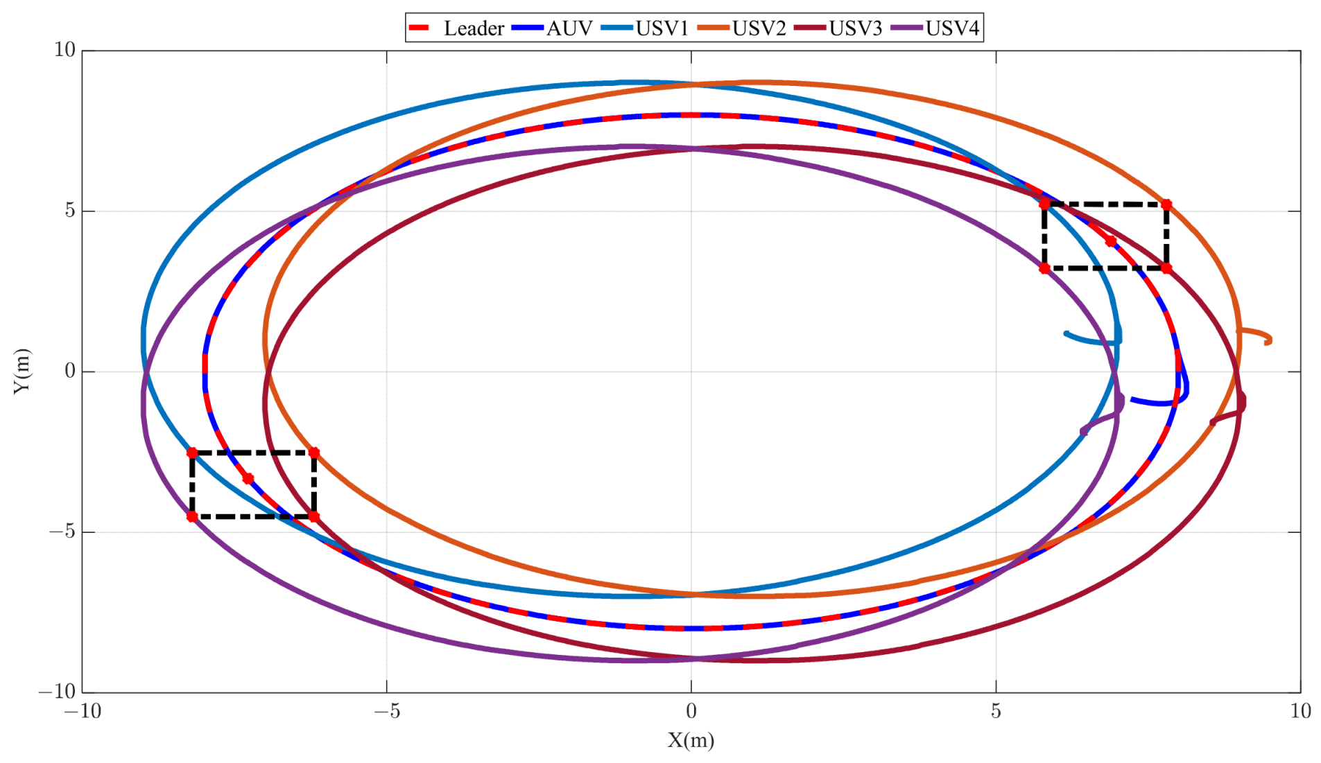
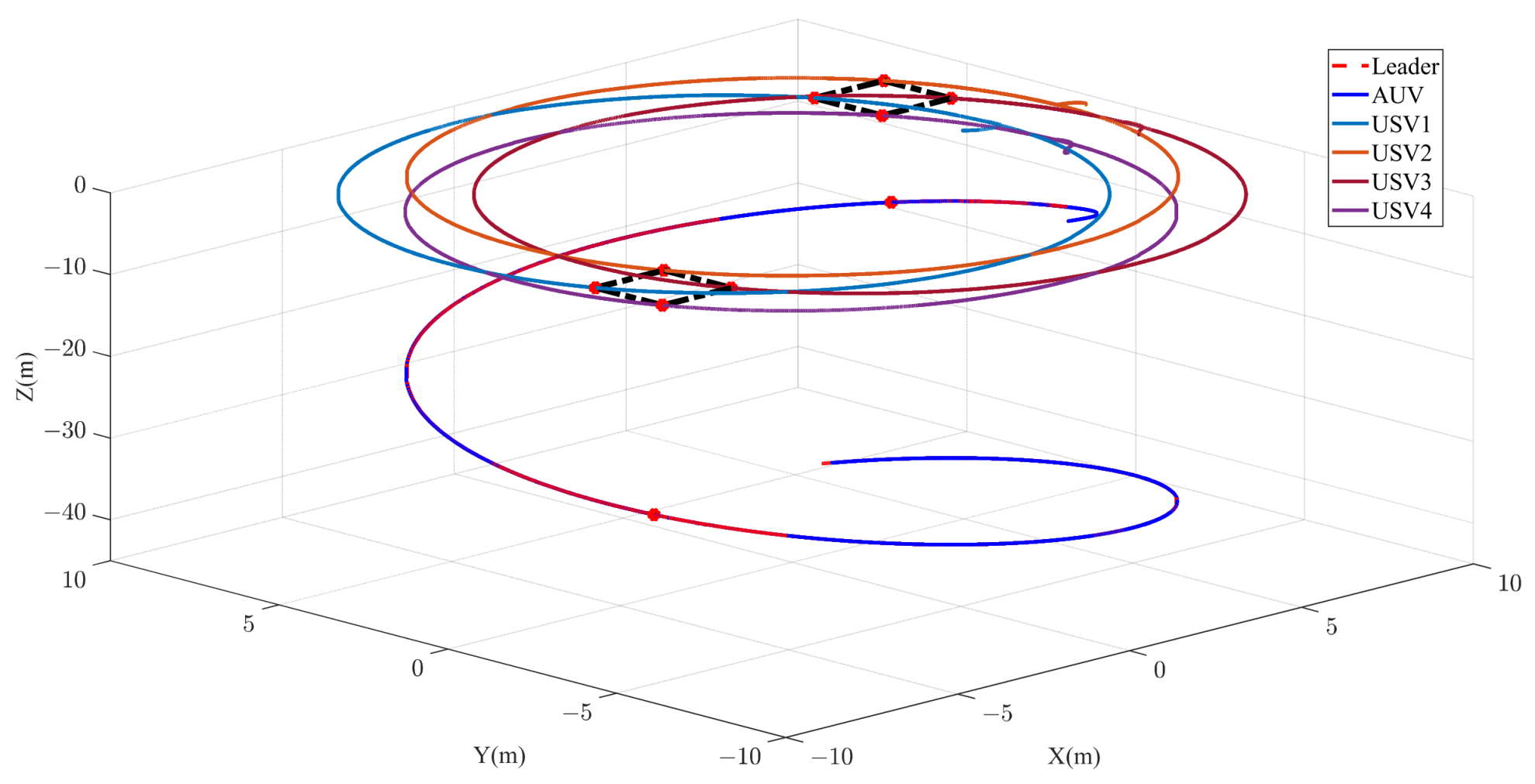
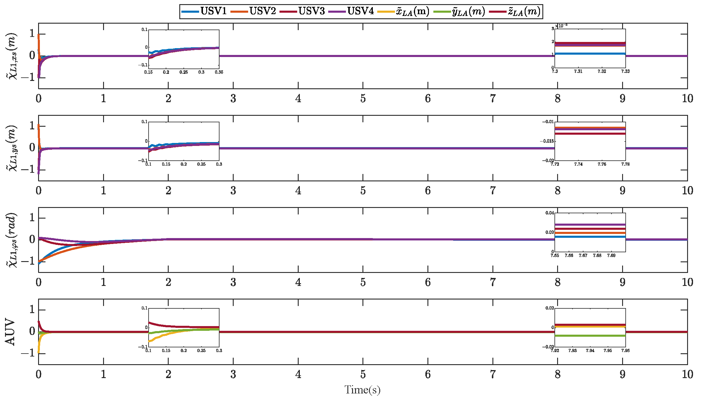
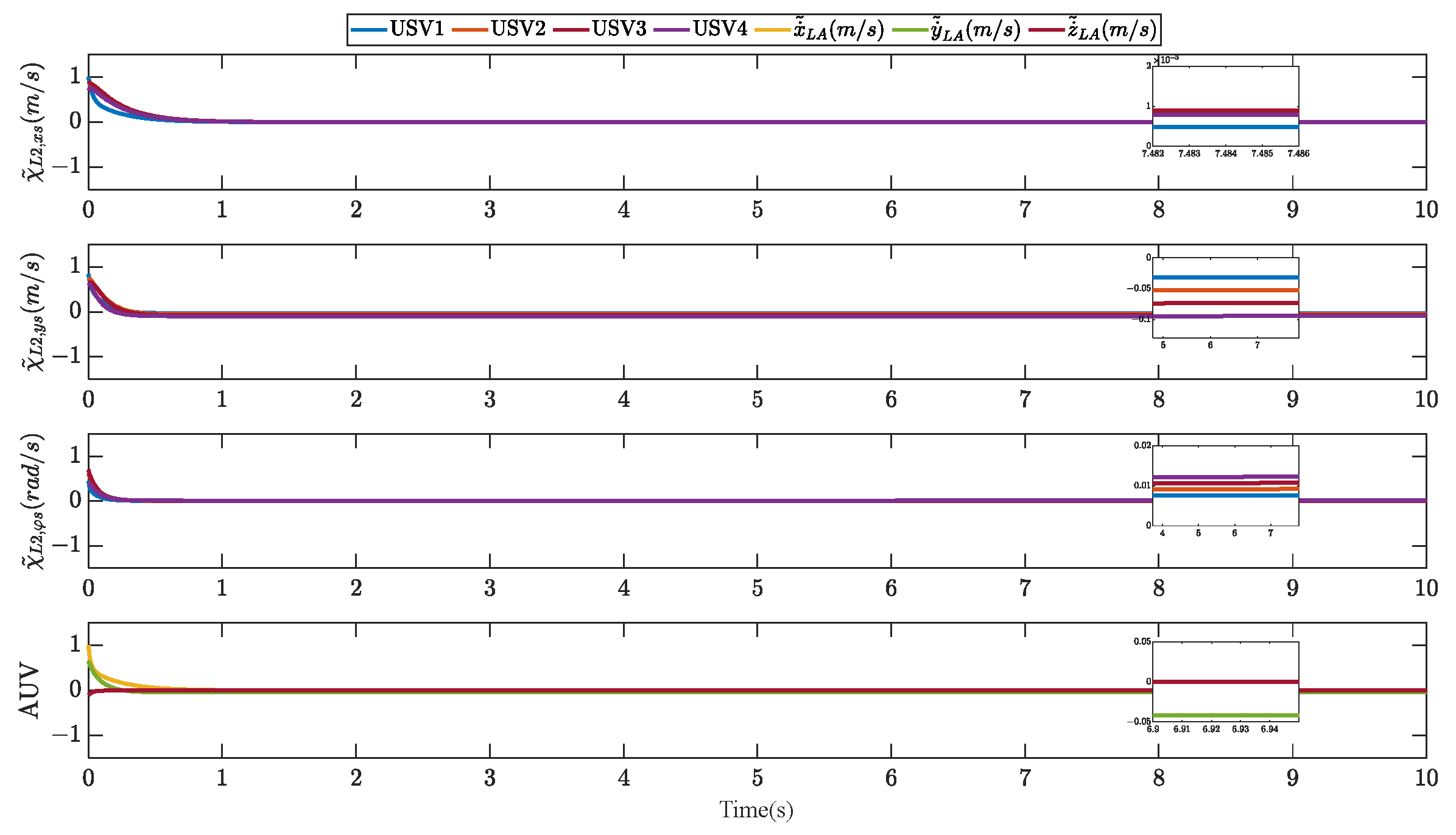
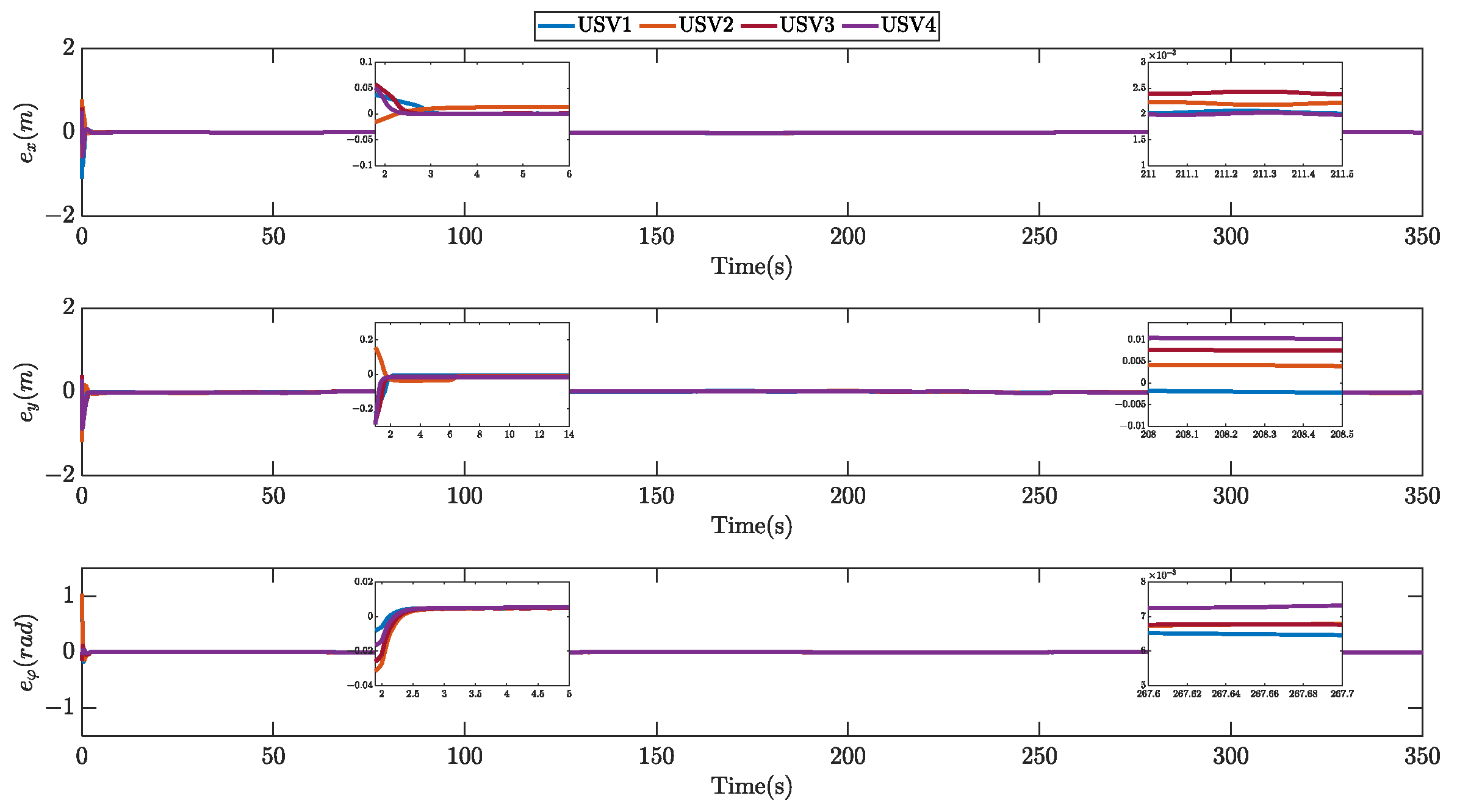
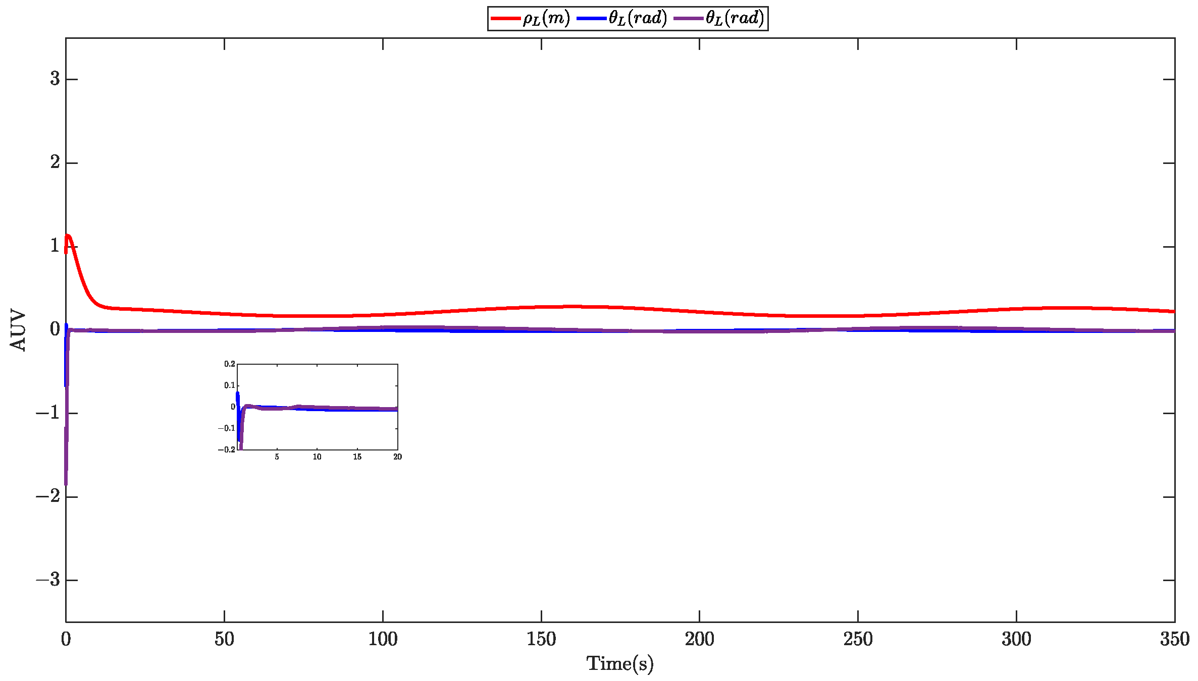
5.2. Simulation Results

The figure below presents the outcomes of the simulations; Figure 5 and Figure 6 represent 2D planar trajectory tracking renderings and 3D stereoscopic trajectory tracking renderings of an underactuated AUV and four USVs at an assumed distance from the virtual leader under the conditions of external environment disturbances, model uncertainty, and actuator input saturation, respectively. The dashed red line depicts the path of the virtual leader, and the other colored solid lines represent the underactuated AUV and the four USVs. In t = 28   s and t = 180   s , the formation configuration is expressed in Figure 5. In this study, the proposed control strategy can realize the control of specific formation requirements and ensure that it can be concluded all the time.
Figure 7 and Figure 8 show the follower’s observed error value of the virtual leader’s state information via PTSO. Figure 7 shows the estimated error values of the underactuated AUV and four USVs for the position information state of the virtual leader. Figure 8 shows the estimated error values for the virtual leader of the underactuated AUV and four USVs for the speed state information. As illustrated in the figure, these values of estimation error for state information are capable of converging close to zero within the predefined time.
Figure 9 and Figure 10 show the tracking error graphs of the four USVs and the underactuated AUV. Figure 11, Figure 12, Figure 13, Figure 14 and Figure 15 show the triggering situation of the memory event-triggered mechanism, Figure 11 shows the triggering situation of USV1, Figure 12 shows the triggering situation of USV2, Figure 13 shows the triggering situation of USV3, Figure 14 shows the triggering situation of USV4, and Figure 15 shows the triggering situation of AUV. Where the x-axis is the triggering time and the y-axis is the triggering time. Figure 16 shows the heterogeneously underactuated AUV-USV system’s control input signal under event-triggering.
In addition, to demonstrate the superiority of the proposed method DRPSC, the proposed method is compared with the fixed-time control algorithm [38] and the traditional sliding mode [47]. In order to comply with the principle of a single variable, all comparative experiments maintain the same expected trajectory, uncertainty disturbances, initial conditions, and parameter configuration.
Figure 17, Figure 18, Figure 19, Figure 20 and Figure 21 show the tracking error graphs of the underactuated AUVs and four USVs under different control methods. Figure 17, Figure 18, Figure 19 and Figure 20 describe the tracking errors for the four USVs, and Figure 21 illustrates the tracking errors of the underactuated AUV. The red solid line signifies the proposed control algorithm DRPSC, the blue solid line signifies the control method of FTSMC, and the purple dashed line represents the traditional SMC method. These figures show that under these three control methods, the tracking errors of different agents can converge within a certain time. In comparison, the proposed method features a shorter convergence time, a faster convergence rate, and a smaller tracking error. This indicates that the proposed formation control algorithm has higher control precision and a better tracking effect.
To further compare the control performance of the three methods, Table 4 summarizes the key performance indicators under the three algorithms, including the convergence time, standard deviation of control forces (SD), and robustness under different disturbance levels (root mean square error (RMSE) of tracking error). Table 5 shows the communication savings situation (including the trigger times and the proportion of communication time) for each control algorithm. Furthermore, in order to compare the robustness under different disturbance levels, the large disturbance value used in the comparative experiment was five times the normal disturbance value adopted in the article.
From this, under three different control algorithms, the proposed DRPSC method has a shorter convergence time; the SD of the control force is smaller, indicating that the proposed method has smaller fluctuations in the control signal and that the system operates smoothly; the trigger times is less and the proportion of communication time is small, suggesting that the proposed method more effectively saves the communication resources of the system; in normal disturbance conditions and large disturbance conditions, the RMSE of the tracking error of the proposed method is less than that of the other two methods, indicating that the proposed method has higher tracking accuracy; and at different disturbance levels, the difference in the RMSE of the tracking error for the proposed method is significantly smaller than that of the other two methods, which further demonstrates that the proposed method has better robustness.
Finally, in Figure 22 and Figure 23, we represent the lumped uncertainty disturbances considered in the system. The impact of the disturbances/uncertainties considered by different agents on the system is similar, and taking USV1 as an example, we show the impact of the considered lumped uncertainty disturbances in Figure 24.
It can be seen from Figure 22 and Figure 23 that the considered disturbances are time-varying. As shown in Figure 24, when USV1 is affected by lumped uncertainty disturbances, the tracking error is larger than the tracking error without the influence of lumped uncertainty disturbances. This indicates that disturbances/uncertainties increase the tracking error of the system and affect the control accuracy of the system.

6. Conclusions

In this research, we studied the formation trajectory tracking issue for underactuated AUV-USV heterogeneous multi-agent systems with external environment disturbances, model uncertainty, and actuator input saturation. For an underactuated AUV-USV system, a distributed predefined-time formation trajectory tracking controller is designed on the basis of a predefined-time control algorithm, distributed PTSO, sliding mode control, H control, an auxiliary dynamic system, and a memory event-triggered mechanism. The distributed PTSO is designed so that each agent can accurately observe the status information of the virtual leader within the predefined time. The use of H control can eliminate external environment disturbances and model uncertainties in an underactuated AUV-USV system and enhance the robustness and stability of the system. Additionally, a PTADS is utilized to alleviate the impact of actuator input saturation, further improving the system’s control accuracy and stability. The system can be stabilized within a predefined time via the DRPSC strategy. The memory event-triggered mechanism can effectively reduce the communication frequency of the underactuated AUV-USV system and economize communication resources. The simulation results demonstrate that the multi-agent system achieves a particular formation configuration in a predefined time. Comparative simulations highlight the significant advantages of the proposed method. However, this study does not consider the obstacle avoidance and delay problems of agents during motion, which is highly important in practical applications, especially in marine environments. When multi-agent systems perform tasks, they may encounter various obstacles, such as seabed topography or other ships, and obstacle avoidance is one of the key issues for ensuring the safety and successful completion of a mission. It requires making decisions and adjusting paths quickly within a short time to address the dynamic marine environment and the irregular movement of obstacles. Moreover, in actual communication among multi-agents, especially in underwater environments, signal transmission may be affected by delay problems, which in turn affect the stability and control performance of the system. Notably, the magnitude of the delay directly affects the response speed of the system. A large delay may lead to a significant decline in system performance and even cause instability. Therefore, it is necessary to study obstacle avoidance and delay problems in multi-agent systems, and future studies will study obstacle avoidance algorithms and delay problems based on heterogeneous multi-agent systems.

Author Contributions

Conceptualization, H.L., L.L. and Q.M.; methodology, H.L. and L.L.; software, L.L.; validation, L.L.; funding acquisition, H.L. and X.T.; resources, X.T. and Q.M.; data curation, Q.M.; writing—original draft preparation, L.L.; writing—review and editing, H.L. and X.T.; supervision, H.L., X.T. and Q.M. All authors have read and agreed to the published version of the manuscript.

Funding

This research was funded by the Guangdong Basic and Applied Basic Research Foundation [grant number 2024A1515011345], the Key Project of the Department of Education of Guangdong Province [grant number 2023ZDZX1005], the Innovation Team Project for Ordinary Universities in Guangdong Province [grant number 2024KCXTD041], the Shenzhen Science and Technology Program [grant number JCYJ20220530162014033], and the Science and Technology Planning Project of Zhanjiang City [grant number 2021A05023].

Data Availability Statement

The original contributions presented in the study are included in the article; further inquiries can be directed to the corresponding author.

Conflicts of Interest

All authors declare that they have no known competing financial interests or personal relationships that could have appeared to influence the work reported in this paper.

References

  1. Zhang, A.; Wang, W.; Bi, W.; Huang, Z. A path planning method based on deep reinforcement learning for AUV in complex marine environment. Ocean Eng. 2024, 313, 119354. [Google Scholar] [CrossRef]
  2. Sun, B.; Niu, N. Multi-AUVs cooperative path planning in 3D underwater terrain and vortex environments based on improved multi-objective particle swarm optimization algorithm. Ocean Eng. 2024, 311, 118944. [Google Scholar] [CrossRef]
  3. Liu, J.; Yu, F.; He, B.; Soares, C.G. A review of underwater docking and charging technology for autonomous vehicles. Ocean Eng. 2024, 297, 117154. [Google Scholar] [CrossRef]
  4. Zhao, L.; Bai, Y. Joint-optimized coverage path planning framework for USV-assisted offshore bathymetric mapping: From theory to practice. Knowl. Based Syst. 2024, 304, 112449. [Google Scholar] [CrossRef]
  5. Zhang, Y.; Wang, Q.; Shen, Y.; Dai, N.; He, B. Multi-AUV cooperative control and autonomous obstacle avoidance study. Ocean Eng. 2024, 304, 117634. [Google Scholar] [CrossRef]
  6. Li, C.; Li, J.; Zhang, G.; Chen, T. IROA-based LDPC-Lévy method for target search of multi AUV–USV system in unknown 3D environment. Ocean Eng. 2023, 286, 115648. [Google Scholar] [CrossRef]
  7. Peng, H.; Hu, J.-S. Traction/Braking Force Distribution for Optimal Longitudinal Motion During Curve Following. Veh. Syst. Dyn. 1996, 26, 301–320. [Google Scholar] [CrossRef]
  8. Mokhiamar, O.; Abe, M. Experimental verification using a driving simulator of the effect of simultaneous optimal distribution of tyre forces for active vehicle handling control. Proc. Inst. Mech. Eng. Part D-J. Automob. Eng. 2005, 219, 135–149. [Google Scholar] [CrossRef]
  9. He, Y.; Chen, Y.; Liu, Y. Event based practical fixed-time consensus control for heterogeneous nonlinear multiagent systems. Inf. Sci. 2023, 650, 119397. [Google Scholar] [CrossRef]
  10. Zhang, X.; Jiang, K. Backstepping-based adaptive control of underactuated AUV subject to unknown dynamics and zero tracking errors. Ocean Eng. 2024, 302, 117640. [Google Scholar] [CrossRef]
  11. Xu, H.; Fossen, T.I.; Guedes Soares, C. Uniformly semiglobally exponential stability of vector field guidance law and autopilot for path-following. Eur. J. Control 2020, 53, 88–97. [Google Scholar] [CrossRef]
  12. Guo, Z.; Zhang, J.; Shang, Y.; Zhang, Y.; Zhang, L.; Chen, W. Predefined-time global recursive sliding mode control for trajectory tracking of unmanned surface vehicles with disturbances uncertainties. Ocean Eng. 2024, 313, 119408. [Google Scholar] [CrossRef]
  13. Li, J.; Zhao, Z.; Qin, X. Adaptive sliding mode control using a novel fully feedback recurrent neural network for quad-rotor UAVs. Neurocomputing 2024, 610, 128592. [Google Scholar] [CrossRef]
  14. Do, K.D.; Pan, J. Global robust adaptive path following of underactuated ships. Automatica 2006, 42, 1713–1722. [Google Scholar] [CrossRef]
  15. Yu, X.; Lin, W. Non-identifier based adaptive control of a chain of integrators and perturbations with unknown delays and parameters. Automatica 2025, 171, 111969. [Google Scholar] [CrossRef]
  16. Wang, Y.; Zhang, H. Lyapunov-based model predictive control for trajectory tracking of hovercraft with actuator constraints and external disturbances. Ocean Eng. 2024, 310, 118631. [Google Scholar] [CrossRef]
  17. Moudoud, B.; Aissaoui, H. Fixed-time adaptive sliding mode-based trajectory tracking control for Wheeled Mobile Robot: Theoretical development and real-time implementation. e-Prime Adv. Electr. Eng. Electron. Energy 2024, 10, 100830. [Google Scholar] [CrossRef]
  18. Moudoud, B.; El Adraoui, I.; Aissaoui, H.; Bahani, A. Fault-Tolerant Control for Wheeled Mobile Robot via Finite-Time Adaptive Sliding Mode. In Proceedings of the 2024 4th International Conference on Innovative Research in Applied Science, Engineering and Technology (IRASET), FEZ, Morocco, 16–17 May 2024; pp. 1–5. [Google Scholar]
  19. Wang, X.; Li, F.; Lee, S.; Shen, H. Event-triggered sliding mode control for interval type-2 fuzzy interconnected systems under Markov-model-based hybrid cyberattacks. Inf. Sci. 2025, 719, 122467. [Google Scholar] [CrossRef]
  20. Sahu, B.K.; Subudhi, B. Flocking Control of Multiple AUVs Based on Fuzzy Potential Functions. IEEE Trans. Fuzzy Syst. 2018, 26, 2539–2551. [Google Scholar] [CrossRef]
  21. Min, H.; Shi, S.; Gu, J.; Duan, N. Further results on fixed-time control for nonlinear systems with asymmetric output constraints. Automatica 2025, 171, 111933. [Google Scholar] [CrossRef]
  22. Jin, X.; Dong, J. Predefined time fuzzy adaptive control for stochastic nonlinear systems with limited time interval output constraints. Inf. Sci. 2025, 689, 121506. [Google Scholar] [CrossRef]
  23. Wu, Z.; Ma, K.; Ni, J. Predefined-time adaptive learning control of nonlinear strict-feedback systems via dynamic regressor extension and mixing. ISA Trans. 2025. [Google Scholar] [CrossRef]
  24. Wang, H.; Shi, S.; Zhen, Z. Flexible performance-based predefined-time tracking control for unmanned helicopter with irregular constraints. Aerosp. Sci. Technol. 2025, 164, 110445. [Google Scholar] [CrossRef]
  25. Guo, G.; Xiao, S.; Chen, F.; Hou, Z.; Tan, H. Dynamic event-triggered predefined-time adaptive attitude fault-tolerant control for uncertain unmanned aerial vehicles with disturbances and actuator faults. Aerosp. Sci. Technol. 2025, 165, 110481. [Google Scholar] [CrossRef]
  26. Liu, H.; Zhou, X.; Tian, X.; Mai, Q.; Sun, N. Predefined-time prescribed performance second-order sliding mode path following control for underactuated marine surface vehicles using self-structuring NN. Ocean Eng. 2024, 309, 118333. [Google Scholar] [CrossRef]
  27. Inoue, D.; Ito, Y.; Kashiwabara, T.; Saito, N.; Yoshida, H. Partially Centralized Model-Predictive Mean Field Games for controlling multi-agent systems. IFAC J. Syst. Control 2023, 24, 100217. [Google Scholar] [CrossRef]
  28. Chen, X.; Hao, F. Event-triggered consensus control of second-order multi-agent systems. Asian J. Control 2015, 17, 592–603. [Google Scholar] [CrossRef]
  29. Talebi, S.P.; Werner, S. Distributed Kalman Filtering and Control Through Embedded Average Consensus Information Fusion. IEEE Trans. Autom. Control 2019, 64, 4396–4403. [Google Scholar] [CrossRef]
  30. Talebi, S.P.; Werner, S.; Gupta, V.; Huang, Y.F. On Stability and Convergence of Distributed Filters. IEEE SIGNAL Process. Lett. 2021, 28, 494–498. [Google Scholar] [CrossRef]
  31. Ding, W.; Zhang, L.; Zhang, G.; Wang, C.; Chai, Y.; Mao, Z. Research on 3D trajectory tracking of underactuated AUV under strong disturbance environment. Comput. Electr. Eng. 2023, 111, 108924. [Google Scholar] [CrossRef]
  32. Liu, H.; Feng, Z.; Tian, X.; Mai, Q. Adaptive predefined-time specific performance control for underactuated multi-AUVs: An edge computing-based optimized RL method. Ocean Eng. 2025, 318, 120048. [Google Scholar] [CrossRef]
  33. Wang, Y.; Song, Y. Leader-following control of high-order multi-agent systems under directed graphs: Pre-specified finite time approach. Automatica 2018, 87, 113–120. [Google Scholar] [CrossRef]
  34. Duan, Q.-S.; Tang, Z.; Ding, D. Distributed adaptive optimal secondary control for AC islanded microgrid under multiple event-triggered mechanisms. ISA Trans. 2025, 163, 65–75. [Google Scholar] [CrossRef]
  35. You, X.; Shi, M.; Guo, B.; Zhu, Y.; Lai, W.; Dian, S.; Liu, K. Event-triggered adaptive fuzzy tracking control for a class of fractional-order uncertain nonlinear systems with external disturbance. Chaos Solitons Fractals 2022, 161, 112393. [Google Scholar] [CrossRef]
  36. Jiang, C.; Zhang, G.; Huang, C.; Zhang, W. Memory-based event-triggered path-following control for a USV in the presence of DoS attack. Ocean Eng. 2024, 310, 118627. [Google Scholar] [CrossRef]
  37. Zhang, H.; Lewis, F.L. Adaptive cooperative tracking control of higher-order nonlinear systems with unknown dynamics. Automatica 2012, 48, 1432–1439. [Google Scholar] [CrossRef]
  38. Gao, Z.; Guo, G. Fixed-time sliding mode formation control of AUVs based on a disturbance observer. IEEE/CAA J. Autom. Sin. 2020, 7, 539–545. [Google Scholar] [CrossRef]
  39. González-Prieto, J.A. Practical fixed-time non-singular sliding mode control of second order nonlinear dynamic systems with chattering and overshooting avoidance. Eur. J. Control 2024, 80, 101114. [Google Scholar] [CrossRef]
  40. Ding, T.-F.; Ge, M.-F.; Xiong, C.; Liu, Z.-W.; Ling, G. Prescribed-time formation tracking of second-order multi-agent networks with directed graphs. Automatica 2023, 152, 110997. [Google Scholar] [CrossRef]
  41. Wang, L.; Chen, C.L.P. Reduced-Order Observer-Based Dynamic Event-Triggered Adaptive NN Control for Stochastic Nonlinear Systems Subject to Unknown Input Saturation. IEEE Trans. Neural Netw. Learn. Syst. 2021, 32, 1678–1690. [Google Scholar] [CrossRef]
  42. Hardy, G.H.; Littlewood, J.E.; Pólya, G. Inequalities; Cambridge University Press: Cambridge, UK, 1952. [Google Scholar]
  43. Dai, Y.; Yang, C.; Yu, S.; Mao, Y.; Zhao, Y. Finite-Time Trajectory Tracking for Marine Vessel by Nonsingular Backstepping Controller With Unknown External Disturbance. IEEE Access 2019, 7, 165897–165907. [Google Scholar] [CrossRef]
  44. Do, K.D.; Pan, J. Design for Underactuated and Nonlinear Marine Systems. In Control of Ships and Underwater Vehicles; Springer Nature: London, UK, 2009. [Google Scholar]
  45. Sui, B.; Zhang, J.; Liu, Z.; Wei, J. Distributed prescribed-time cooperative formation tracking control of networked unmanned surface vessels under directed graph. Ocean Eng. 2024, 305, 117993. [Google Scholar] [CrossRef]
  46. Liu, H.; Tian, X.; Wang, G.; Zhang, T. Robust H∞ finite-time stability control of a class of nonlinear systems. Appl. Math. Model. 2016, 40, 5111–5122. [Google Scholar] [CrossRef]
  47. El Khazane, J.; Tissir, E.H. Achievement of MPPT by finite time convergence sliding mode control for photovoltaic pumping system. Sol. Energy 2018, 166, 13–20. [Google Scholar] [CrossRef]
Figure 1. Scenario diagram of the underactuated AUV-USV system.
Jmse 13 01428 g001
Figure 2. DRPSC block diagram.
Jmse 13 01428 g002
Figure 3. Communication network topology.
Jmse 13 01428 g003
Figure 4. Underactuated AUV-USV formation.
Jmse 13 01428 g004
Figure 5. 2D track tracking rendering of the underactuated AUV-USV.
Jmse 13 01428 g005
Figure 6. 3D space track tracking rendering of the underactuated AUV-USV.
Jmse 13 01428 g006
Figure 7. Position estimation error of the observer.
Jmse 13 01428 g007
Figure 8. Velocity estimation error of the observer.
Jmse 13 01428 g008
Figure 9. Tracking errors of the four USVs.
Jmse 13 01428 g009
Figure 10. Tracking errors of the AUV.
Jmse 13 01428 g010
Figure 11. Event-triggered interevent times of USV1.
Jmse 13 01428 g011
Figure 12. Event-triggered interevent times of USV2.
Jmse 13 01428 g012
Figure 13. Event-triggered interevent times of USV3.
Jmse 13 01428 g013
Figure 14. Event-triggered interevent times of USV4.
Jmse 13 01428 g014
Figure 15. Event-triggered interevent times of the AUV.
Jmse 13 01428 g015
Figure 16. Control input of the underactuated AUV-USV system.
Jmse 13 01428 g016
Figure 17. Tracking errors of USV1 under different control methods.
Jmse 13 01428 g017
Figure 18. Tracking errors of USV2 under different control methods.
Jmse 13 01428 g018
Figure 19. Tracking errors of USV3 under different control methods.
Jmse 13 01428 g019
Figure 20. Tracking errors of USV4 under different control methods.
Jmse 13 01428 g020
Figure 21. Tracking errors of the underactuated AUV under different control methods.
Jmse 13 01428 g021
Figure 22. Lumped uncertainty disturbances of the four USVs.
Jmse 13 01428 g022
Figure 23. Lumped uncertainty disturbances of the AUV.
Jmse 13 01428 g023
Figure 24. Diagram of the impact of lumped uncertainty disturbances.
Jmse 13 01428 g024
Table 1. Model parameter information of the underactuated AUV.
SymbolValueSymbolValue
m 1 ( kg ) 25.00 d 1 ( kg s 1 ) 30.00
m 2 ( kg ) 17.50 d 2 ( kg s 1 ) 30.00
m 3 ( kg ) 30.00 d 3 ( kg s 1 ) 30.00
m 5 ( kg m 2 ) 22.50 d 5 ( kg s 1 ) 20.00
m 6 ( kg m 2 ) 15.00 d 6 ( kg s 1 ) 20.00
ρ g Δ G ¯ M ¯ L 5.00 Δ d i , a m , Δ m i , a m , Δ G , m ( i = 1 , 2 , 3 , 5 , 6 ) 0.1
Table 2. Model parameter information of the USVs.
SymbolValueSymbolValue
m 11 m X u ˙ c 31 , k c 13 , k
m 22 m Y v ˙ c 32 , k c 23 , k
m 23 m x g Y r ˙ d 11 , k X u X u u u s k X u u u u s k 2
m 32 m x g N v ˙ d 22 , k Y v Y v v v s k Y r v r s k
m 33 I Z N r ˙ d 23 , k Y r Y v r v s k Y r r r s k
c 13 , k m 22 v s k m 23 r s k d 32 , k N v N v v v s k N r v r s k
c 23 , k m 11 u s k d 33 , k N r N v r v s k N r r r s k
Table 3. Hydrodynamic parameter information of the model.
SymbolValueSymbolValueSymbolValue
m 23.8 Y v 0.8612 N v 0.1052
I Z 1.76 Y v v 36.2823 N v v 5.0437
x g 0.046 Y r v 8.05 N r v 0.13
X u ˙ 2.0 Y r ˙ 0 N r ˙ 1.0
X u 0.7225 Y r 0.1079 N r 1.9
X u u 1.3274 Y v r 0.845 N v r 0.08
X u u u 5.8664 Y r r 3.45 N r r 0.75
Y v ˙ 10.0 N v ˙ 0
Table 4. Performance evaluation under different control methods.
DRPSC/FTSMC/Traditional SMC
Convergence Time (s)SD of Control Inputs (N)RMSE of Tracking Errors
Normal Disturbance (m)Large Disturbance (m)
USV1x5/15/156.6720/18.0863/18.32470.0321/0.0716/0.07120.0370/0.1060/0.1007
y5/15/153.4357/13.2030/13.33100.0242/0.0302/0.02960.0276/0.0571/0.0510
φ 3/6/73.5073/14.9712/14.84170.0191/0.0217/0.02150.0212/0.0234/0.0235
USV2x5/15/155.7180/18.2679/18.41010.0225/0.0339/0.03390.0292/0.0448/0.0484
y5/15/152.8891/12.6037/12.64300.0356/0.0221/0.02180.0379/0.0388/0.0417
φ 3/6/73.2316/14.3522/14.45680.0187/0.0261/0.02600.0208/0.0278/0.0293
USV3x5/10/106.0189/13.3098/8.69960.0150/0.0440/0.04350.0240/0.0751/0.0746
y5/15/155.0535/11.2161/12.06890.0543/0.0549/0.05430.0557/0.0867/0.0865
φ 3/6/71.1838/20.4412/22.96650.0059/0.0095/0.00980.0109/0.0133/0.0183
USV4x5/15/156.3733/6.8035/6.89770.0188/0.0500/0.04960.0266/0.0816/0.0834
y5/15/155.9358/14.2980/14.37250.0723/0.0757/0.07510.0733/0.1121/0.1140
φ 3/6/70.8599/21.6587/21.81730.0066/0.0076/0.00760.0113/0.0146/0.0219
AUV ρ 15/40/805.3334/17.7609/18.44820.2255/1.1604/2.09290.2350/0.8690/2.2084
θ 5/15/1813.3637/18.5128/43.60150.0261/0.0773/0.06760.0304/0.1930/0.1234
φ 3/15/3010.7234/12.3839/10.75100.0684/0.1479/0.27860.0685/0.1545/0.4719
Table 5. Communication situation under different control methods (total sampling data: 35,000).
DRPSCFTSMCTraditional SMC
Trigger TimesPercentageTrigger TimesPercentageTrigger TimesPercentage
τ x s 1 4111.17%31939.12%34759.93%
τ y s 1 11523.29%1071930.62%1087931.08%
τ φ s 1 4951.41%662018.91%741221.18%
τ x s 2 3360.96%31619.03%32159.19%
τ y s 2 6741.93%1104031.54%1108531.67%
τ φ s 2 5231.49%615917.60%614417.55%
τ x s 3 3691.05%31969.13%32119.17%
τ y s 3 5741.64%1124932.14%1119731.99%
τ φ s 3 5431.55%624817.85%644618.42%
τ x s 4 3951.13%30568.73%30678.76%
τ y s 4 12663.62%1119531.98%1130532.30%
τ φ s 4 4971.42%844524.13%820523.44%
τ u A 24497.00%396211.32%673019.23%
τ q A 7362.10%660918.88%977527.93%
τ r A 12103.46%678819.39%683719.53%
Disclaimer/Publisher’s Note: The statements, opinions and data contained in all publications are solely those of the individual author(s) and contributor(s) and not of MDPI and/or the editor(s). MDPI and/or the editor(s) disclaim responsibility for any injury to people or property resulting from any ideas, methods, instructions or products referred to in the content.

