Article

Nonparametric Prediction of Ship Maneuvering Motions Based on Interpretable NbeatsX Deep Learning Method

by
Lijia Chen
1,2,3,*,
Xinwei Zhou
1,2,3,
Kezhong Liu
1,
Yang Zhou
1 and
Hewei Tian
4
1
School of Navigation, Wuhan University of Technology, Wuhan 430063, China
2
Hubei Key Laboratory of Inland Shipping Technology, Wuhan University of Technology, Wuhan 430063, China
3
State Key Laboratory of Maritime Technology and Safety, Wuhan University of Technology, Wuhan 430063, China
4
ChangJiang Pilot Center, Changshu 215500, China
*
Author to whom correspondence should be addressed.
J. Mar. Sci. Eng. 2025, 13(8), 1417; https://doi.org/10.3390/jmse13081417
Submission received: 30 June 2025 / Revised: 18 July 2025 / Accepted: 23 July 2025 / Published: 25 July 2025
(This article belongs to the Section Ocean Engineering)

Abstract

With the development of the shipbuilding industry, nonparametric prediction has become the mainstream method for predicting ship maneuvering motion. However, the lack of transparency and interpretability make the output process of the prediction results challenging to track and understand. An interpretable deep learning framework based on the NbeatsX model is presented for nonparametric ship maneuvering motion prediction. Its three-tier fully connected architecture incorporates trend, seasonal, and exogenous constraints to decompose motion data, enhancing temporal and contextual learning while rendering the prediction process transparent. On the KVLCC2 zig-zag maneuver dataset, NbeatsX achieves NRMSEs of 0.01872, 0.01234, and 0.01661 for surge speed, sway speed, and yaw rate, with SMAPEs of 9.21%, 6.40%, and 7.66% and R2 values all above 0.995, yielding a more than 20% average error reduction compared with LS-SVM, LSTM, and LSTM–Attention and reducing total training time by about 15%. This method unifies high-fidelity forecasting with transparent decision tracing. It is an effective aid for ship maneuvering, offering more credible support for maritime navigation and safety decision-making, and it has substantial practical application potential.

1. Introduction

Predicting ship maneuvering motion constitutes a fundamental area of research within maritime traffic and safety. Given the rapid advancements in maritime autonomous surface ships (MASSs) [1], the ability to accurately forecast ship maneuvering behavior has become critically important. This predictive capability is essential for ensuring both efficient and safe navigation, as well as for supporting the development of reliable decision-making processes related to ship maneuvers [2]. For example, it is important for cargo transportation, helicopter take-off and landing, and ship “pairing” between large transport vessels and small ships. If the trends and deterministic values of ship motion can be obtained 5 to 10 s in advance, explosions caused by cargo collisions can be prevented during cargo transfers, and landing times can be calculated during helicopter landings to avoid accidents [3].
Methods for predicting ship maneuvering motion are diverse, with the most prevalent approaches being parametric and nonparametric prediction methods. Parametric prediction methods use prior knowledge to establish a mathematical model of maneuvering motion; these are combined with hydrodynamic parameters, which indicate the physical mechanisms of the ship maneuvering motion. The unknown parameters in the mathematical model should be accurately determined based on captive model tests, simulations with prescribed ship motions, or system identification for parametric modeling. Several methods can be used for this approach, such as the Kalman filter [4], ordinary least squares [5], support vector machines [6], least squares support vector machines [7], etc. In parametric prediction methods, a substantial number of parameters are typically established to accurately represent such model structures. Although these meaningful parameters can be determined through identification algorithms and incorporated into the original model for maneuvering motion predictions [8,9], the extensive quantity of parameters requiring identification coupled with the complex parameter identification process often necessitates considerable computational time. Consequently, this may hinder efforts to achieve rapid and precise predictions of ship maneuvering motion.
While parametric prediction methods can clearly and intuitively illustrate the influence of various physical quantities on ship motion, they evidently fall short in meeting contemporary demands for accuracy and efficiency in predicting ship maneuvering motion [10]. The nonparametric prediction method does not presuppose a fixed, finite set of parameters or a predetermined functional form for the data-generating process, and it does not need any prior knowledge about the ship dynamic system [11]. By discarding the constraints of the fixed model architecture and fitting the system, a mapping relationship between the input and output can be obtained to establish the model and thereby rapidly predict the ship’s maneuvering motion [12]. Model flexibility and adaptability to complex, nonlinear relationships are essential for nonparametric prediction. Deep learning methods employ artificial neural networks to automatically extract high-level abstract features through multi-layered representation learning; this capacity to learn hierarchical, data-driven mappings without assuming any fixed functional form underpins their dominant role in nonparametric prediction.
Recurrent neural networks (RNNs), particularly their variant known as long short-term memory (LSTM) networks [13,14], have exhibited exceptional performance in time series prediction tasks due to their distinctive architecture. Prediction accuracy is a critical evaluation metric in prediction problems. Particularly, with the introduction and ongoing refinement of attention mechanisms [15], the accuracy of nonparametric prediction methods for ship maneuvering motion has been significantly improved by integrating this complex yet highly efficient mechanism. Zhang et al. [16] introduced multi-scale attention to augment the performance of long short-term memory (LSTM) networks in ship motion prediction, validating the method’s accuracy and generalizability using experimental data that incorporated artificial noise. Wang et al. [17] combined a bi-directional long short-term memory network with a self-attention mechanism and one-dimensional convolution, proposing a nonparametric prediction method for ship maneuvering motion named SeaBil, which demonstrated high accuracy in ultra-short-term predictions. One of the notable advantages of deep learning methods in addressing time series prediction challenges is their capacity to enhance model performance through adjustments to model depth. When focusing solely on the accuracy and efficiency of output results in forecasting, it becomes evident that continuously deepening the model structure has yielded excellent outcomes to a certain extent. Indeed, if emphasis is placed exclusively on these aspects within predictive modeling, then progressively enhancing model depth has proven effective up to a point. However, this does not align well with the research purpose of ensuring the safety of vessels when forecasting ship maneuvering movements [18]. This means that the credibility of the forecast results is greatly diminished—even if the forecast is accurate ninety-nine times, decision-makers may still not be completely convinced by the hundredth forecast. The increasingly complex model structure significantly reduces its interpretability, making the process of outputting forecast results more difficult to understand, and the inherent stochasticity and the absence of systematic evaluation frameworks further obscure the path to practical deployment [19]. This is also why many outstanding prediction methods in the fields of finance, healthcare, and transportation continue to emerge, yet their actual industrial applications are infrequent.
The “black box” nature of nonparametric prediction methods does not imply that the decision-making process of the model is entirely incomprehensible [20] or beyond study. Interpretability aims to understand the logical reasoning behind the mappings of nonparametric models rather than just knowing how the results are calculated through a series of meaningless values (weights). The key to achieving interpretability lies in using transparent, easy-to-understand model structures or providing clear, logical chains [21], making the model’s decision-making process traceable and comprehensible. This paper proposes a nonparametric prediction method for ship maneuvering motion based on the interpretable deep learning NbeatsX model. Unlike RNN-, CNN-, or transformer-based time series predictors, the NbeatsX backbone relies exclusively on fully connected layers, yielding a simpler and more transparent network topology. This design facilitates the direct decomposition of inputs into trend, seasonal, and exogenous contributions without complex mechanisms, thereby greatly enhancing interpretability. At the same time, the removal of recurrent or convolutional operations reduces the number of trainable parameters and accelerates inference, which is critical for real-time ship maneuvering applications. The main contributions of this paper are as follows:
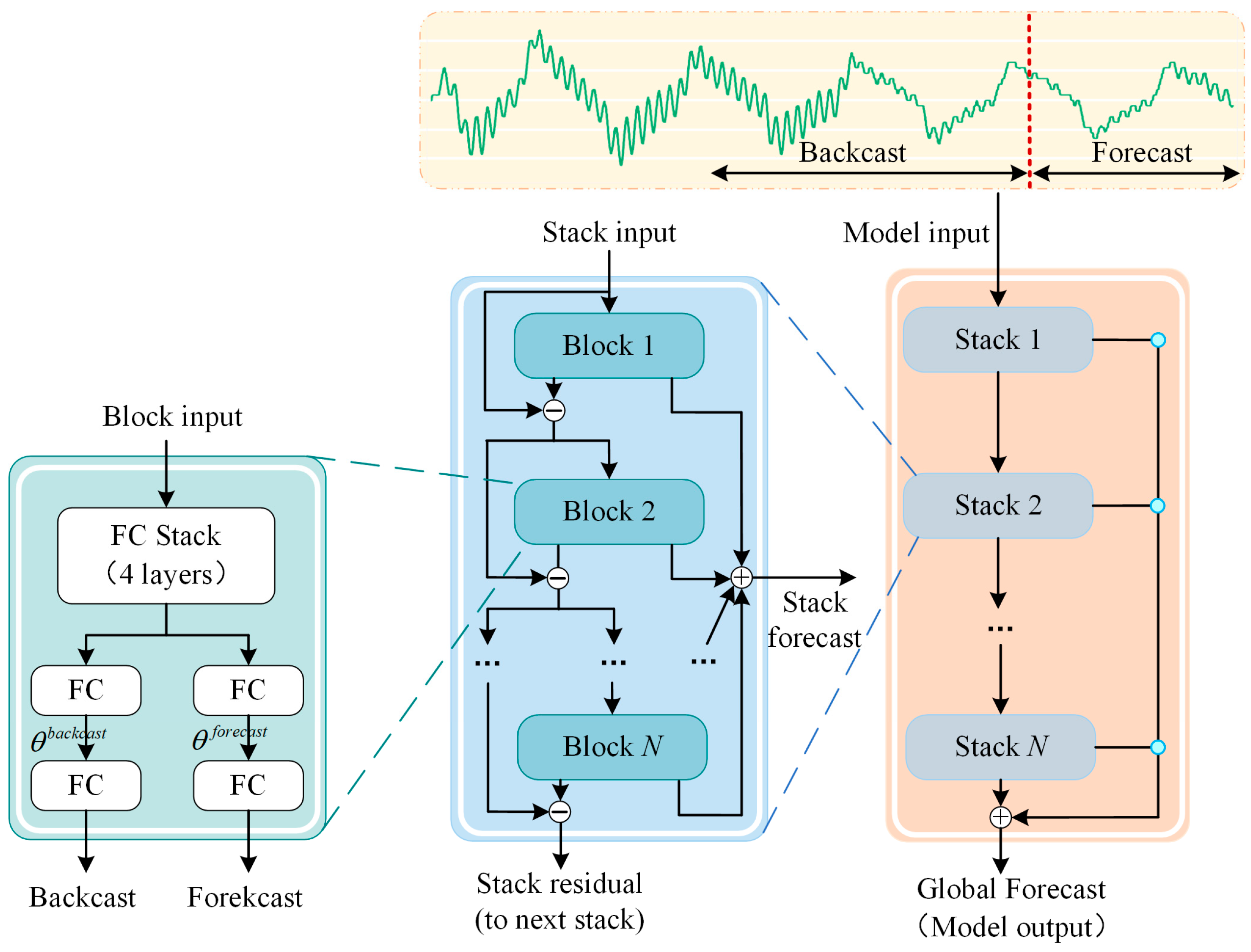
  • Simple, general, and expressive model architecture: The architecture comprises a novel backbone built exclusively from fully connected layers, organized into block and stack modules. Block layers employ residual connections to iteratively backcast input signals, while stack layers aggregate multi-horizon forecasts and backcasts, enabling efficient time series feature learning without recurrent or convolutional operations.
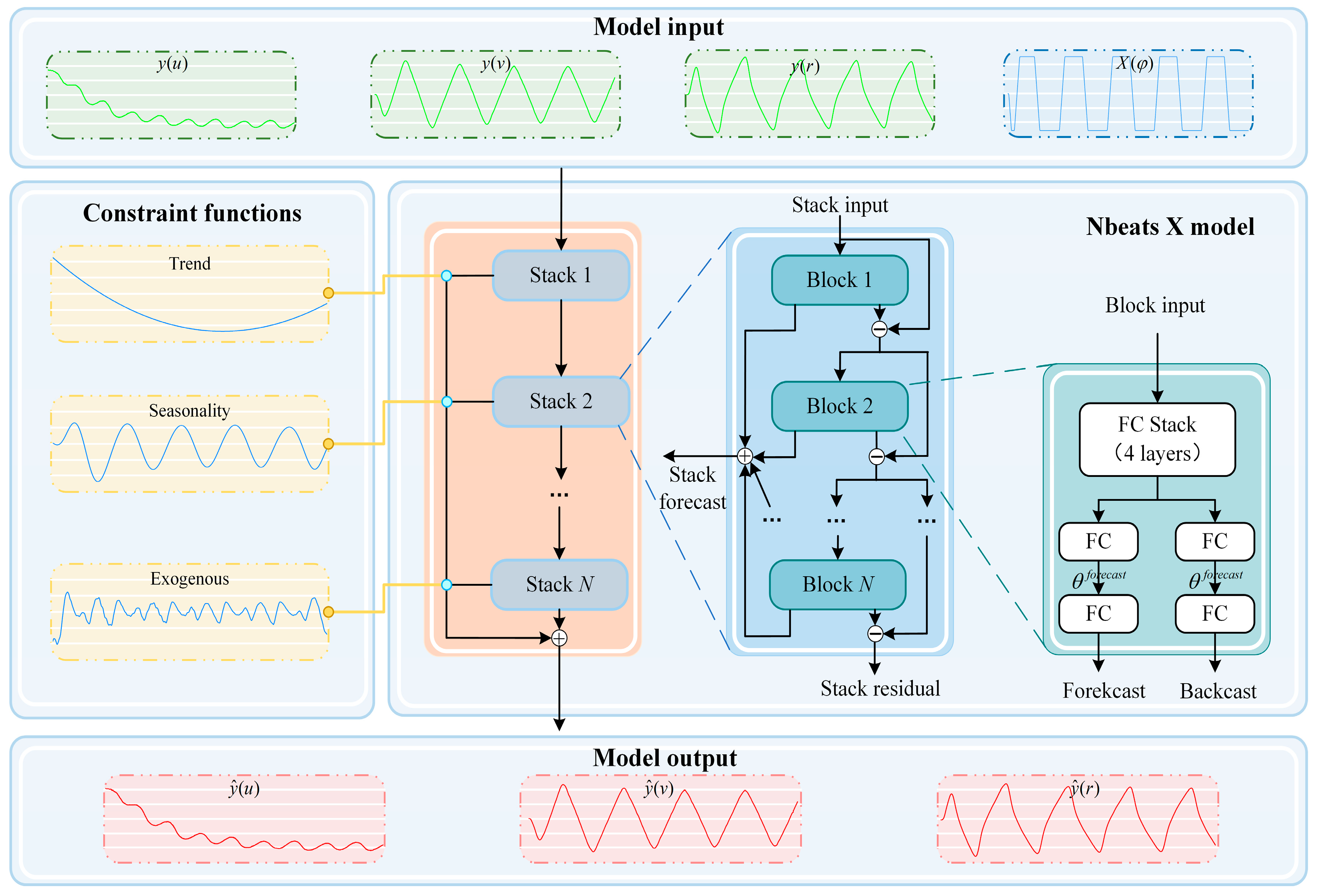
  • Interpretable time series signal decomposition: Based on the stack structure of the NbeatsX model, through the establishment of flexible prediction modules with stack restrictions, it is feasible to select classic time series feature functions such as trend, seasonality, and expansion factor functions to jointly construct precise and interpretable prediction outcomes.
  • Results and discussion based on the KVLCC2 dataset: The model’s prediction accuracy is validated using KVLCC2 ship model data obtained from SIMMAN workshop benchmark test cases. A dedicated interpretability module then decomposes each prediction into trend, seasonal, and exogenous contributions, providing clear and actionable insights into the model’s decision process.
The rest of the paper is organized as follows: Section 2 constructs a nonparametric model for ship maneuvering motion and deals with the interpretability issues of nonparametric prediction methods for ships. Section 3 introduces the fundamental architecture of the NbeatsX model and the implementation of its interpretability features. Section 4 uses the KVLCC2 dataset to present and discuss the prediction results of the NbeatsX model. Section 5 presents the conclusions and suggestions for future work.

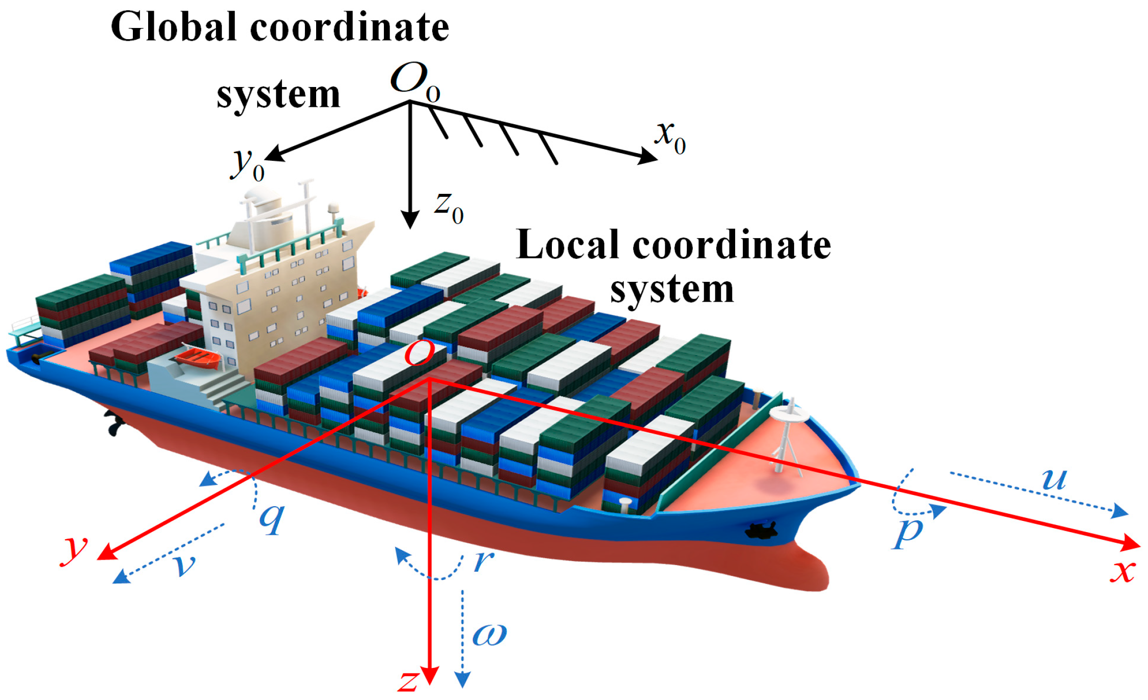
2. Nonparametric Ship Maneuvering Model

Generally, ship maneuvering prediction can be formulated as multi-input–multi-output high-dimensional system modeling, which achieves ship motion prediction by capturing the nonlinear relationships among input variables and output variables. Nonparametric models are better at representing complex nonlinear factors and coupling information on ship motion states [22], making them a primary focus of current research.
Typically, to nonparametrically predict ship maneuvering motion, it is essential to first determine the input and output data, as illustrated in Figure 1, where O o - x o y o z o represents the global coordinate system, O - x y z represents the local coordinate system, u , v , ω denote the surge, sway, and heave speeds, and r , p , q represent the pitch, roll, and yaw angular speeds.
Ships exhibit six degrees of freedom in their motion on the water surface. However, the study of ship maneuverability focuses primarily on three degrees of freedom, namely surge, sway, and yaw. In the ship motion coordinate system, the three-degree-of-freedom equations for ship maneuvering can be expressed as shown in Equation (1) [23]:
m ( u ˙ v r + x G r 2 ) = X m ( v ˙ + u r + x G r ˙ ) = Y I z z r ˙ + m x G ( v ˙ + u r ) = N
where m represents the ship’s mass, u ˙ represents the longitudinal acceleration, v ˙ represents the lateral acceleration, and r ˙ represents the yaw acceleration. x G is the coordinate of the ship’s center of gravity along the longitudinal axis, and I z z is the moment of inertia around the vertical axis. X , Y , N indicate the longitudinal forces, lateral forces, and yaw moments. Equation (1) can be initially transformed to establish a nonparametric model, as described in Equation (2) [24]:
m X u ˙ 0 0 0 m Y v ˙ m x G Y r ˙ 0 m x G N v ˙ I z z N r ˙ u ˙ v ˙ r ˙ = f 1 ( u , v , r , δ ) f 2 ( u , v , r , δ ) f 3 ( u , v , r , δ )
where X u ˙ , Y v ˙ , Y r ˙ , N v ˙ , and N r ˙ are hydrodynamic derivatives of inertia, δ is the rudder angle, and f is a linear function connected with u , v , r , and δ . Further processing of Equation (2) leads to Equation (3):
u ˙ = f 4 ( u , v , r , δ ) v ˙ = f 5 ( u , v , r , δ ) r ˙ = f 6 ( u , v , r , δ )
The longitudinal acceleration, lateral acceleration, and yaw acceleration are discretized using the forward difference method:
u ˙ = ( u ( t + 1 ) u ( t ) ) / h v ˙ = ( v ( t + 1 ) v ( t ) ) / h r ˙ = ( r ( t + 1 ) r ( t ) ) / h
where h represents the sampling interval, and t + 1 and t represent consecutive sampling times. By substituting the discretized accelerations from Equation (4) into Equation (3), the final equation is obtained:
u ( t + 1 ) = f 7 u ( t ) , v ( t ) , r ( t ) , δ ( t ) v ( t + 1 ) = f 8 u ( t ) , v ( t ) , r ( t ) , δ ( t ) r ( t + 1 ) = f 9 u ( t ) , v ( t ) , r ( t ) , δ ( t )
The three-degree-of-freedom ship maneuvering motion is converted into a nonparametric model through the aforementioned nonlinear processing and structural simplification. This model uses the current moment’s values of u , v , r , δ as input data x and the next moment’s values of u , v , r as output data y . This relationship is represented in Equation (6):
x = [ u , v , r , δ ] y = [ u , v , r ]
Referring to [24], the input data sequences are [ u ( t ) , v ( t ) , r ( t ) , δ ( t ) ] , where the target feature is y = [ u ( t ) , v ( t ) , r ( t ) ] and external feature is δ ( t ) . The predicted output results are therefore y ^ = [ u ( t + 1 ) , v ( t + 1 ) , r ( t + 1 ) ] . Data from five time steps are uniformly used to ensure a balance between prediction accuracy and efficiency.
Theoretically, by selecting the appropriate forecasting method and continuously improving it, it is possible to fit the nonlinear mapping between inputs and outputs, achieving high-precision, nonparametric predictions of ship maneuvering movements. While ongoing improvements in the model increase the accuracy of predictions to some extent, the progressively complex structure of the model also deepens its “black box” nature. The decision-making process becomes more challenging to interpret, and the credibility of the predicted results is questioned. This is a persistent but often overlooked issue in the field of time series prediction. Specifically in ship maneuvering prediction, the credibility of results is crucial. Therefore, the NbeatsX model proposed in this paper is completely constructed based on fully connected layers. Its straightforward structure achieves lower time complexity and memory utilization. Meanwhile, the added interpretable decomposition module can clearly show the entire process from data input to output, as well as the proportion of the influence of input data on the test results, effectively guaranteeing the accuracy and credibility of the results.

3. Proposed Method

3.1. Input Matrix Based on Spatiotemporal Features

The NbeatsX (Neural Basis Expansion Analysis for Interpretable Time Series X) model is a deep learning method for time series prediction. Distinguished from the three mainstream time prediction model frameworks, RNNs, CNNs, and transformers, NbeatsX pioneers a new backbone, utilizing only fully connected neural networks (FCNNs) to perform time series predictions. This approach renders the model structure more transparent, simple, and efficient. Its superior capability in time series prediction has been verified in multiple fields such as the electricity market [25,26], financial volatility [27], macroeconomics, and ecology [28], demonstrating strong predictive capabilities and excellent explanatory power. The NbeatsX model features three key characteristics, which are simplicity, versatility, and expressive power (depth). Firstly, the model framework is simple and universal yet possesses substantial expressive capabilities. Secondly, the model is independent from specific time series feature engineering or input scaling. This trait allows for the exploration of deep learning model structures and their potential in time series prediction. Thirdly, the model structure is designed to be interpretable.
The NbeatsX model performs time series decomposition through multiple layers of fully connected networks, with each layer fitting a part of the time series information. The model’s core consists of multiple stack modules, each of which is further made up of several blocks connected in series. Each block, as the fundamental structural unit of NbeatsX, comprises four fully connected neural network layers and one linear layer. The first block in each stack receives the raw input sequence, and each block thereafter operates on the residual remaining after subtracting the previous block’s backcast output. Every block produces a backcast component, which removes its fitted portion from the residual, and a forecast component, which is accumulated across all blocks to form the final prediction. The final output of NbeatsX is the summation of outputs from all stacks. The basic structure of the model is illustrated in Figure 2.
In each block of the NbeatsX model, whether it is for forecasting or the reconstruction of the backcast, two processes are involved, namely mapping the input time series to expansion coefficients and then mapping these coefficients back to the time series. These expansion coefficients can be understood as low-dimensional vectors that store time series information, akin to the vector mapping process in an AutoEncoder, which involves mapping the input time series into a low-dimensional vector, then mapping it back to the time series. Referring to [29], this process can be represented as Equations (7) and (8):
f m , n = F c n n m , n ( y m , n 1 )
θ m , n b a c k c a s t = L i n e a r b a c k c a s t ( f m , n ) ,   θ m , n f o r e c a s t = L i n e a r f o r e c a s t ( f m , n )
where f m , n represents the hidden units between fully connected layers, with m and n as specific position or dimension indices, F c n n represents the fully connected neural network, y represents the input data, θ b a c k c a s t and θ p r e d i c t represent the expansion coefficients for past reconstruction and future predictions, respectively, and L i n e a r represents a linear layer.
In the NbeatsX model, for each block, the process involves the following steps, where each block generates two sets of expansion coefficients, which are then combined with the corresponding base vectors through expansion operations to yield specific reconstructed and predicted values [30], as described in Equation (9):
y ˜ m , n b a c k c a s t = V m , n b a c k c a s t θ m , n b a c k c a s t ,   y ˜ m , n f o r e c a s t = V m , n f o r e c a s t θ m , n f o r e c a s t
where y ˜ b a c k c a s t and y ˜ f o r e c a s t represent the components of past reconstruction and future predictions obtained through expansion coefficient operations and base vectors, with V b a c k c a s t and V f o r e c a s t representing the respective base vectors.
The time series data computed by each block model is input into the stack, employing the principle of double-residual stacking for data accumulation, which can also be seen as a sequential decomposition of the model signal. In this way, each layer of the stack handles the residuals that the previous layer could not fit correctly, effectively decomposing the time series layer by layer. The calculated residuals also serve as input variables for the next level of prediction. The formula for calculating prediction residuals is shown in Equation (10):
y m , n + 1 b a c k c a s t = y m , n b a c k c a s t y ˜ m , n b a c k c a s t
where y m , n + 1 b a c k c a s t represents the residual backcast of the m , n +1-th stack.
In the NbeatsX model, each stack aggregates the forecast components y ˜ m , n f o r e c a s t from its respective blocks and outputs the final forecast result as Equation (11):
y ˜ f o r e c a s t = n = 1 N y ˜ m f o r e c a s t
where y ˜ f o r e c a s t represents the final forecast result obtained by the summation of all the stack predictions.
In most nonparametric ship maneuvering motion prediction research, a structured input–output approach is adopted to ensure the efficiency of the prediction. For instance, if the input and output data are [ u ( t + 1 ) , v ( t + 1 ) , r ( t + 1 ) ] , it is clear that the data in the input sequence can be divided into two main categories, namely target features [ u ( t ) , v ( t ) , r ( t ) ] that require prediction and external features [ φ ( t ) , δ ( t ) ] that do not, as shown in Equation (6). From a data science perspective, these two different sets of features each contain distinct information. Although convenient, the traditional method of inputting them together without processing may reduce the information utilization rate and lead to issues like feature confusion or omission. Therefore, the NbeatsX model further processes the input sequence, splitting it into forecast features and exogenous features. Both are passed through fully connected layers to obtain a hidden state, which is then used to generate expansion coefficients. Building on Equation (7), the input data features are split into target and external features, leading to Equation (12):
f m , n = F c n n m , n ( y m , n 1 , X n 1 )
where y represents the target features and X represents the external features.
This input processing strategy preserves temporal dependencies, enhances feature utilization, and delivers unprecedented interpretability in neural forecasting models. By isolating target series from exogenous inputs, NbeatsX learns distinct patterns within each data type, yielding both higher accuracy and a clearer attribution of predictive influences.

3.2. Interpretable Configuration

When configuring the base functions within the stack of the NbeatsX model, the primary characteristics of time series data to be considered are trend [31], seasonality [32], and exogenous factors, which can also be called residuals [33]. By incorporating prior knowledge into the stack architecture, the model constrains the expansion coefficients to extract specific characteristics of the input data’s time series. Specifically, polynomial terms are used to model trends, seasonal harmonic functions capture periodic patterns, and covariates account for residual factors. This approach ensures that the model accurately fits the time series data while enhancing the interpretability of the results. The explainable configuration is mathematically described by Equations (13)–(15).
y ˜ m , n t r e n d = i = 0 P t i θ m , n , i t r e n d
y ˜ m , n s e a s o n a l i t y = i = 0 H / 2 1 c o s ( 2 π i t h ) θ m , n , i s e a s o n a l i t y + s i n ( 2 π i t h ) θ m , n , i + H / 2 s e a s o n a l i t y
y ˜ m , n e x o g e n o u s = i = 0 N x λ i θ m , n , i e x o g e n o u s
where y ˜ t r e n d , y ˜ s e a s o n a l i t y , and y ˜ e x o g e n o u s , respectively, represent the trend, seasonality, and exogenous factors derived from the decomposition. t i = [ 0 , 1 , 2 , , H ] / H , H represents the step length of the time series, h represents a hyperparameter that suppresses harmonics, λ represents the feature vector λ = [ λ 1 , λ 2 , , λ N x ] , and N x represents the number of feature variables.
To facilitate the understanding of the system, Algorithm 1 provides pseudocode for using the interpretability module to predict ship maneuvering motion.
Algorithm 1: Using the interpretable module for predicting ship maneuvering motion.
  Input: Dataset// Ship maneuvering motion dataset ( y m , n 1 , X n 1 ) ;
b, f, epochs // b for external feature sequences length, f for target feature sequence length
   V T f o r e c a s t ,    V T b a c k c a s t // The basic parameter vector of the calculated trend
   V S f o r e c a s t , V S b a c k c a s t // The basic parameter vector of the calculated seasonality
   V E f o r e c a s t , V E b a c k c a s t // The basic parameter vector of the calculated exogenous
t = shape ( V T f o r e c a s t )[0], s = shape ( V S f o r e c a s t )[0],
e = shape ( V E f o r e c a s t )[0];
  while epoch < epochs do
  index = [random(0 – len(Dataset), b)]
  x = Dataset[index]; //using index as a pointer
  y = Dataset[index + f][−f];
  forecast = x, residuals = x;
  while i < number of blocks do
     if block == T then
         θ = FCNN(residuals);// expansion coefficient
        block_forecast = θ [: t] * V T f o r e c a s t ;
        block_backcast = θ [t :] * V T f o r e c a s t ;
     if block == S then
         θ = FCNN(residuals);
        block_forecast = θ [: s] * V S f o r e c a s t ;
        block_backcast = θ [s :] * V S b a c k c a s t ;
     if block == E then
        theta = FCNN(residuals);
        block_forecast = θ [: e] * V E f o r e c a s t ;
        block_backcast = θ [e :] * V E b a c k c a s t ;
     residuals = (residuals –block_backcast);
      y ^ = residuals + block_forecast; // the prediction results
     i++;
  Get cost function of ( y ^ , y);
  epoch++;
Algorithm 1 begins by initializing the interpretable NbeatsX_STEE module with its three base vectors for trend, seasonality, and exogenous dynamics, along with the hyperparameters b, f, and epochs. At each training epoch, a random segment of length b is sampled from the ship maneuvering motion dataset to form the input x; the corresponding ground-truth target y consists of the next f steps following this segment. The forecast output and the residual signal are both initialized to x. Within each block of the stacked architecture, the current residuals are passed through a fully connected network (FCNN) to produce a block-specific coefficient vector θ . If the block is designated as a trend (T), the first t elements of θ are multiplied by the trend basis to yield the block’s forecast contribution and the remaining elements by the trend basis to produce its backcast; analogous operations are performed for seasonal (S) and exogenous (E) blocks using their respective basis lengths s and e. After computing each block’s backcast, the residuals are updated by subtracting the backcast, and the forecast is accumulated by adding the block’s forecast contribution.
This process repeats across all blocks, resulting in a final multi-component prediction for the current mini-batch. The mean squared error between the aggregated forecast and the true target y is then computed as the cost, and gradients are backpropagated through the entire stack to update all FCNN and basis parameters via the chosen optimizer. The epoch counter increments, and the cycle continues until the specified number of epochs is reached or early stopping criteria are met.

3.3. Nonparametric Prediction Method Based on Nbeatsx

The input to the first module includes lagged data from the target feature sequence, as well as external feature sequences. In contrast, the input to each subsequent module incorporates residual connections derived from the backward prediction output of its preceding module. Initially, the NbeatsX framework conducts separate local nonlinear projections on the input data, effectively decomposing the target signal into base functions associated with different blocks. Each block consists of a fully connected neural network that learns expansion coefficients for both backcast and forecast elements. The backcast model serves to refine inputs for subsequent blocks, while forecasts are aggregated to produce the final prediction result. Data blocks are organized in a stacked format; within this structure, each stack may be oriented towards processing numerous variants of base functions across potentially multiple stacks.
NbeatsX processes a sliding window of recent measurements equal in length to the backcast horizon, enabling predictions with minimal computational overhead and high throughput. Each stack then applies its learned trend, seasonal, and exogenous basis functions to generate individual forecast components, and these components are summed to produce the final output. By feeding only the local segments of both target and external inputs, the model captures long-term dependencies through its exogenous branch while preserving full transparency for each additive contribution. Figure 3 presents the complete nonparametric prediction pipeline for ship maneuvering motion, illustrating how the outputs from all stacks combine to form a coherent forecast.

4. Results and Discussion

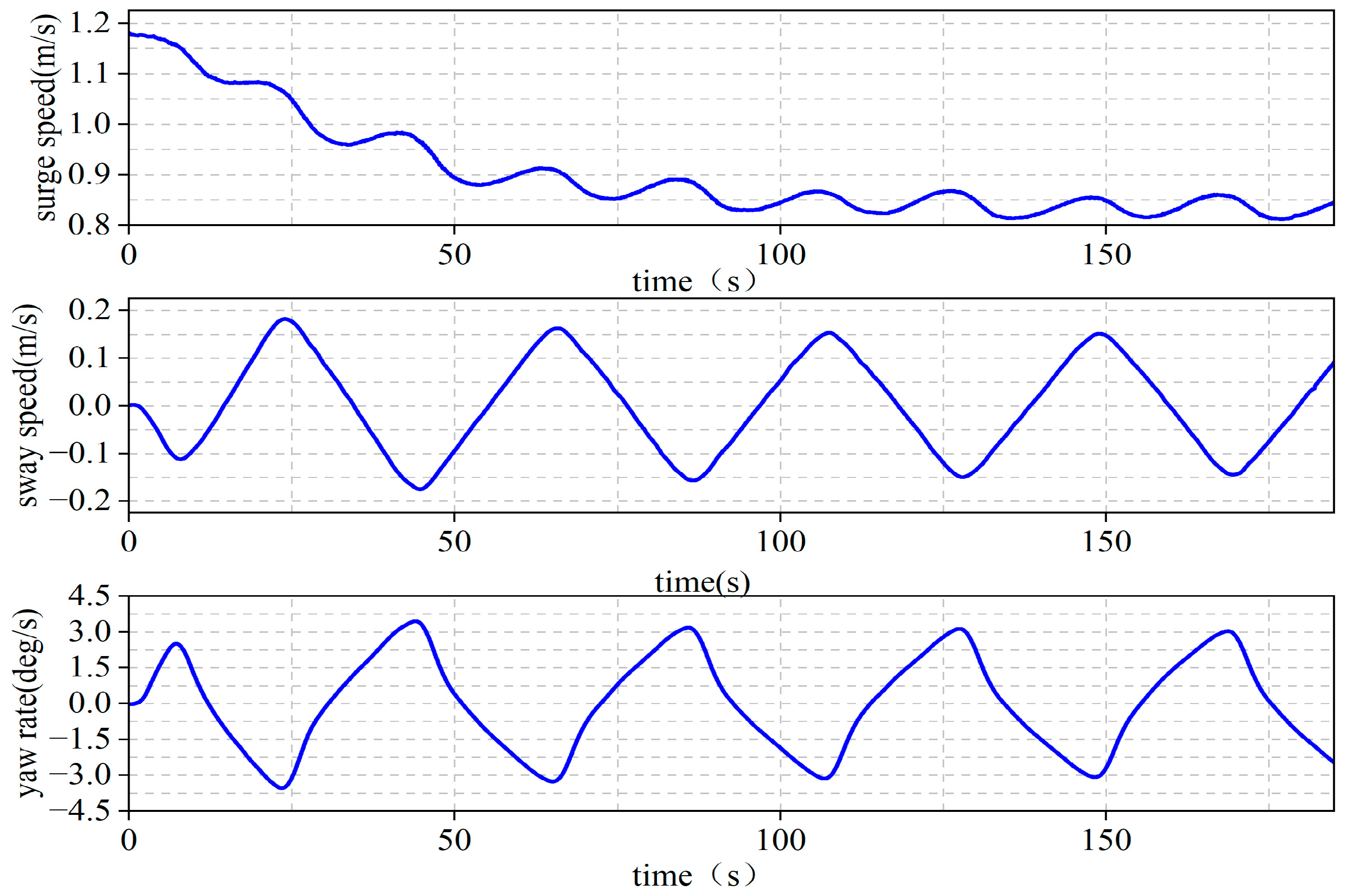
4.1. Data Description and Preparation

The experimental environment setup is shown in Table 1. To ensure that the dataset provides sufficient stimulation for model training and testing, a dataset composed of real-world test data from the KVLCC2 model was selected [34]. These data are applied by various institutions and are widely used in ship maneuverability research. Table 2 compares the parameters between the ship model and full scale. [35]
The KVLCC2 dataset includes six independent zig-zag maneuver datasets, as shown in Figure 4. The data of 10°/5°, 15°/5°, 20°/5°, and 30°/5° zig-zag maneuvers were selected as the training dataset. The 35°/5° zig-zag maneuver was selected as the validation data. The 25°/5° zig-zag maneuver was selected as the testing data for out-of-sample testing, as shown in Figure 5.
x = x x max x max x min
where x′ is the scaled variable, x is the original variable, and xmax and xmin are the maximum and minimum values of the variable.
To optimize performance on the validation set, key hyperparameters, including mini-batch size, the number of epochs, learning rate, and optimizer, were selected by grid search over predefined ranges, choosing the combination that minimized validation loss. Conducting a grid search over 32, 64, and 128 batch sizes; 200, 500, and 800 epochs; and 1 × 10⁻², 1 × 10⁻³, and 1 × 10⁻⁴ learning rates, the configuration with the lowest validation NRMSE was selected. The final configuration used a batch size of 64, 500 epochs, an initial learning rate of 1 × 10⁻³, and the Adam optimizer.

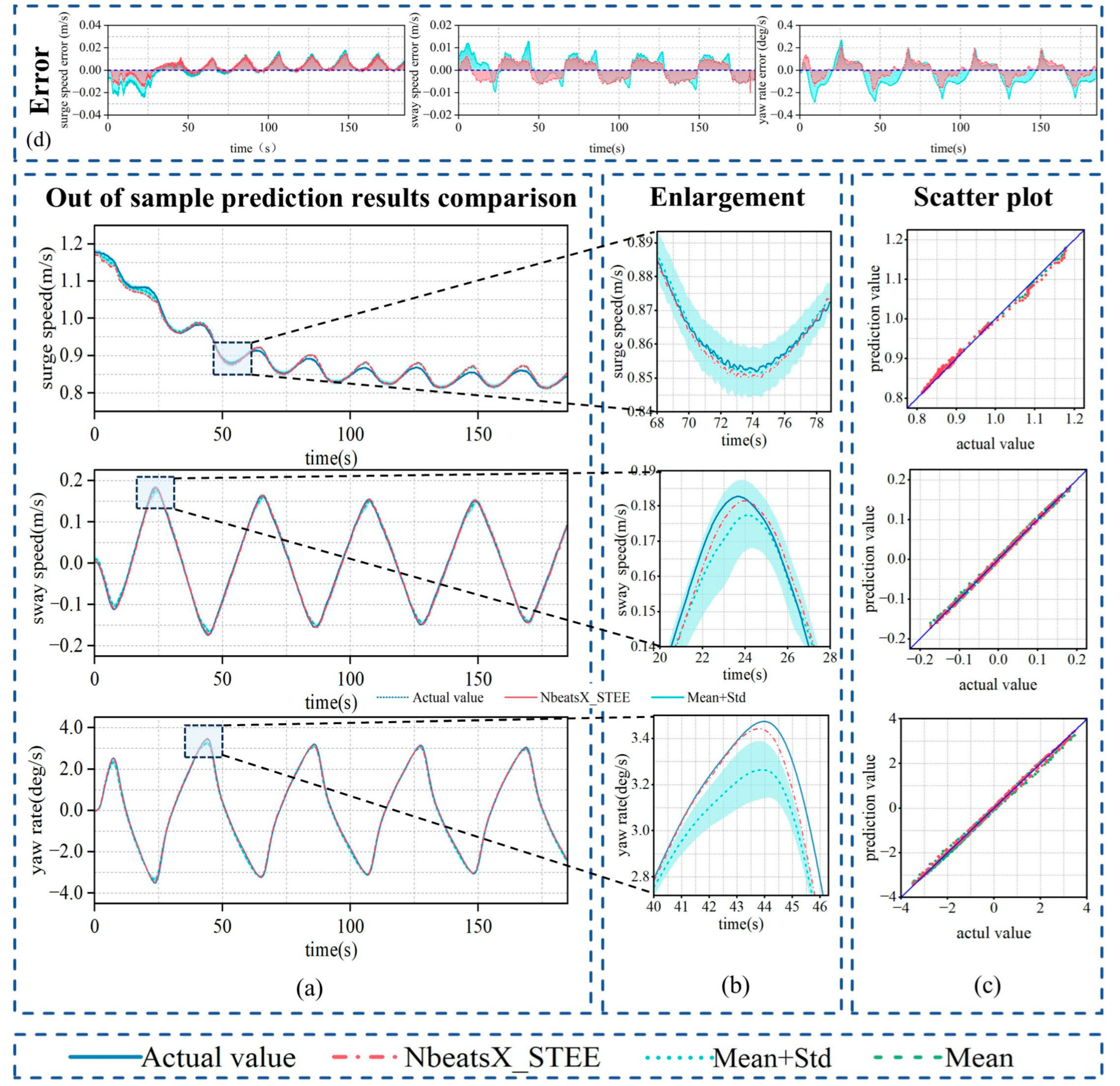
4.2. Prediction Results and Discussion

This paper employs the normalized root mean square error (NRMSE), symmetric mean absolute percentage error (SMAPE), and coefficient of determination (R2) as evaluation metrics [36] to provide a more comprehensive understanding of model performance. Lower values of the NRMSE and SMAPE indicate higher prediction accuracy, whereas a higher R2 suggests the opposite; the NRMSE, SMAPE, and R2 are defined in Equations (17)–(19):
NRMSE = 1 N i = 1 N y ^ i y i 2 y max y min
SMAPE = 100 % N i = 1 N y ^ i y i y ^ i + y i / 2
R 2 = 1 i = 1 N y i y ^ i 2 i = 1 N y i y ¯ 2
where y i represents the true observed value of the i-th sample, y ^ i represents the predicted value, y ¯ = 1 N i = 1 N y i represents the mean value, and N represents the number of test samples.
To fully demonstrate and validate the effectiveness and superiority of the NbeatsX model used in this paper, it is compared and analyzed against the LS-SVM model [37], LSTM model [38], and LSTM–Attention model [16], which are recognized for their excellent performance in handling time series prediction problems.
Figure 6 illustrates a comparison of nonparametric prediction results in three degrees of freedom between the NbeatsX model and other baseline models. To facilitate more detailed examination and provide an intuitive representation of the distribution of prediction outcomes, an enlarged view is included alongside scatter plots depicting different models’ prediction results. Figure 6a presents a comparison of the prediction results; Figure 6b provides an enlarged comparison; and Figure 6c displays scatter plots comparing predicted results against actual outcomes.
Combining the prediction results presented in Figure 6 with the quantitative evaluation metrics provided in Table 3, an analysis of specific prediction outcomes reveals that the NbeatsX model exhibits exceptional predictive capabilities for sway speed ( v ) and yaw rate ( r ), which display more pronounced periodicity and amplitude characteristics. This model significantly outperforms other baseline models regarding accuracy. For instance, as indicated in Table 3, the SMAPE result for the yaw rate achieved by the NbeatsX model is 7.25%, which is considerably lower than those of alternative models.
However, it is noteworthy that the prediction accuracy of the NbeatsX model for surge speed ( u ) is relatively lower compared to other baseline models. For instance, taking the normalized root mean square error (NRMSE) as an example, the NRMSE result for surge speed prediction by the NbeatsX model is 0.04088, which is significantly higher than the value of 0.03303 achieved by the LSTM–Attn model. The primary reason for this discrepancy lies in the fact that while the NbeatsX model excels at handling nonlinear and complex patterns through its architecture of stacked fully connected layers, it may struggle to effectively capture subtle changes in data with small magnitudes such as surge speed. These minor fluctuations are more continuous and less pronounced, leading to a decrease in prediction accuracy. This characteristic becomes particularly evident when examining sway speed predictions; although sway speed also has a smaller magnitude, it exhibits more regular and intuitive frequency fluctuations. The NbeatsX model successfully captures these characteristics and achieves high prediction accuracy in this context, yielding superior results across metrics such as the NRMSE, SMAPE, and R2. In summary, while the NbeatsX model proposed in this paper generally demonstrates commendable predictive performance regarding KVLCC2 ship maneuvering motion, its inherent structural limitations suggest there remains potential for enhancing predictive effectiveness. Further exploration and analysis are needed to improve its performance in this regard.
The NbeatsX model innovates by stacking layers constrained by trend (T), seasonality (S), and exogenous (E) functions and then concatenating their outputs to form the final prediction. In addition to the original general purpose configuration, four variants, NbeatsX_TES, NbeatsX_TSE, NbeatsX_STE, and NbeatsX_STEE, were designed to better capture specific data characteristics such as surge speed. Figure 7 presents the prediction results for the structural variations in the NbeatsX model, providing a more intuitive understanding of prediction accuracy by calculating the mean and standard deviation of the prediction results from four different structural configurations of the NbeatsX models. Additionally, we display the prediction outcomes for the most complex NbeatsX_STEE model. The mean prediction results across different structural models underscore the credibility of the NbeatsX framework, while the standard deviation serves to indicate its confidence interval.
From Figure 7a, it is evident that, despite modifications in the model structure, the models consistently maintain a high level of accuracy. Table 4 presents a comparison of errors between the prediction results from various structural NbeatsX models and actual KVLCC2 ship data. This comparison indicates that the error in motion response predictions by the expanded NbeatsX models is somewhat reduced, further validating the credibility of this approach. For instance, when considering the normalized root mean square error (NRMSE), the results for NbeatsX_TES, NbeatsX_TSE, and NbeatsX_STE models are 0.03887, 0.03591, and 0.03441, respectively. Although these figures represent improvements over NbeatsX’s score of 0.04088, they still exceed LSTM–Attn’s result of 0.03303. This finding reinforces previous analyses concerning the low sensitivity of the NbeatsX model to small-magnitude fluctuations.
However, while the NbeatsX_STEE variant—constructed by sequentially stacking trend, seasonal, and exogenous blocks—demonstrates the robust mitigation of data volatility in surge speed prediction, its performance also highlights the subtle trade-offs introduced by deeper architectures. Greater depth can enrich representational capacity but also increases parameter count, heighten the risk of overfitting when data are limited, and can exacerbate gradient vanishing or explosion during training. Moreover, since the underlying data signals may have different characteristic deviations, such as having a much stronger trend and seasonality, the introduction of excessive exogenous blocks would compromise the overall accuracy. This complexity is reflected in sway speed prediction: the deeper NbeatsX_STEE records an NRMSE of 0.01661, whereas the shallower NbeatsX_STE achieves a lower error of 0.01311. Such a reversal indicates that additional layers may capture redundant or conflicting features. Balancing the depth and composition of stacks to align with the dominant characteristics of the data is therefore critical. A comprehensive exploration of these trade-offs will guide future work in identifying optimal configurations for diverse maneuvering scenarios.
To illustrate these trade-offs, Figure 8, Figure 9 and Figure 10 present decomposition and reconstruction examples. The left column shows the individual outputs of the trend, seasonal, and exogenous stacks, and the right column overlays the NbeatsX_STEE reconstruction on the actual measurements. Figure 8 shows that the trend in surge speed dominates, while the exogenous output remains nearly flat. Figure 9 shows that the actual fluctuation amplitude of the sway speed is relatively small, and the trend component and seasonal component can already capture the main patterns. However, NbeatsX_STEE additionally stacked an exogenous factor module. The decomposition panel (the orange curve) then exhibited more high-frequency fluctuations. These subtle noises introduced by the exogenous stack were indiscriminately incorporated into the prediction results during reconstruction. Figure 10 shows moderate contributions from all three components. Due to the large magnitude of the yaw rate, the exogenous stack captures minor noise that slightly perturbs the prediction. In this case, the deeper STEE configuration offers no clear advantage over STE, reinforcing the conclusion that stacking should be tailored to each signal’s dominant characteristics. Therefore, stack depth and composition must reflect the signal’s dominant characteristics; over-stacking a weakly expressed component can introduce spurious detail and affects the accuracy of the prediction.
For rigorous comparisons, it is essential to evaluate the time consumption associated with the proposed model. Table 5 presents the training and prediction times for various structural NbeatsX models in comparison to other baseline models. The time expenditure of these models primarily arises during the training phase. Among them, the traditional machine learning model LS-SVM exhibits the least time consumption, at approximately 326.069 s. The overall time consumption for different structural NbeatsX models is relatively consistent, averaging around 350 s each. In contrast, both the LSTM model and its more complex variant, LSTM–Attn, require significantly more time, with 354.870 s and 408.345 s, respectively. In terms of efficiency, the training duration of the NbeatsX model is markedly reduced; it successfully completes 4200 predictions in under 0.2 s. While this performance may be influenced by computational capabilities, such prediction times are deemed acceptable within practical contexts. Overall, the NbeatsX model demonstrates high predictive accuracy and efficiency while maintaining robust stability—surpassing both traditional and state-of-the-art models in ship motion prediction tasks. This underscores its potential as a valuable tool for predicting and analyzing ship maneuvering motion in real-world applications.
Leveraging the function-fitting ability to perform an interpretability analysis of the prediction results and formulating reasonable hypotheses is an effective way to advance academic discussion [39]. The interpretability of NbeatsX enables it to make more profound contributions to developing ship maneuvering motion prediction. Specifically, its significance can be summarized in several key aspects as follows:
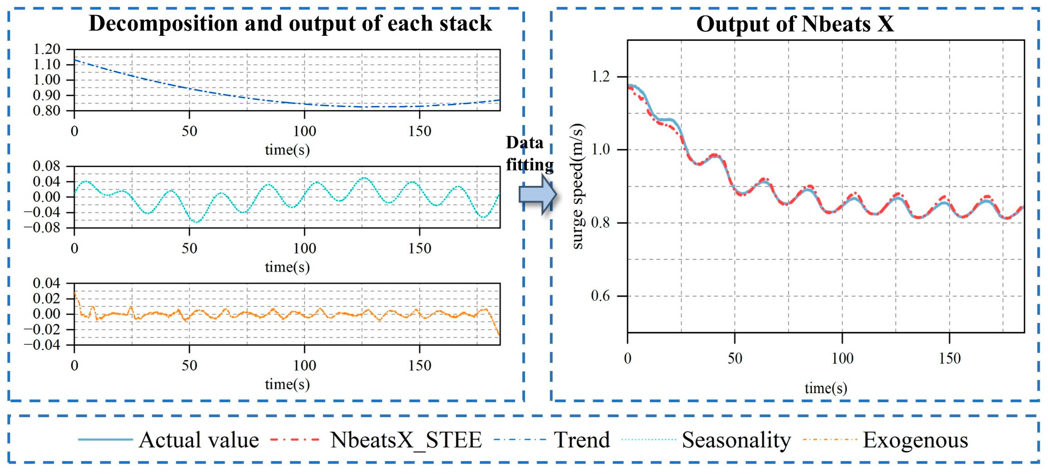
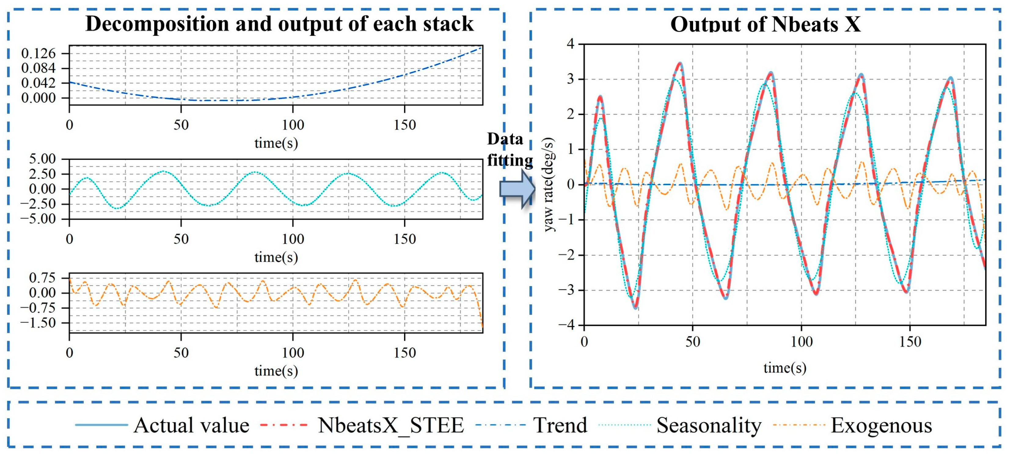
  • Engineering perspective: From an engineering perspective, NbeatsX conducts decomposition processing based on the prescribed basis functions and subsequently integrates the decomposed data to form the final prediction outcome. This implies the addition of “constraints” to the deep learning model, for instance, the necessity to employ polynomial functions for fitting. Moreover, these constraints are typically interpretable (e.g., periodic and polynomial functions).
  • Clearer understanding of ship motion patterns: NbeatsX offers a transparent and streamlined architecture. Its stack modules, each configured with trend, seasonal, or exogenous basis functions, enable the model to isolate and examine specific motion characteristics. For instance, fitting the seasonal stack reveals the cyclic behavior of ship maneuvers, while the trend stack exposes longer-term tendencies across different degrees of freedom.
  • Interface for advanced ship maneuvering motion research: The stack structure of the NbeatsX model provides an interface for more specialized research in ship maneuvering motion. For instance, setting specific computational formulas as the general function constraints in the exogenous factors stack could help analyze unobserved variables or random noise, revealing information the model might have overlooked.

5. Conclusions

Seeking the accurate prediction of ship motion dynamics, this paper presents the NbeatsX deep learning method that demonstrates high prediction accuracy and strong interpretability. On the KVLCC2 zig-zag maneuver dataset, the NbeatsX achieves NRMSEs of 0.01872, 0.01234, and 0.01661 for surge speed, sway speed, and yaw rate, with SMAPEs of 9.21%, 6.40%, and 7.66% and R2 values all above 0.995, yielding a more than 20% average error reduction compared with LS-SVM, LSTM, and LSTM–Attention and reducing the total training time by about 15%. Its built-in interpretability module can decompose each prediction into trend, seasonal, and exogenous contributions, making the decision process transparent. These results show that stacking constraints according to signal characteristics delivers simultaneous gains in accuracy, efficiency, and explainability, offering a practical tool for enhanced navigational safety and maneuvering assistance.
In future work, data augmentation methods such as jittering, cropping, and injection will be integrated into the dataset to enhance model generalization. The resilience of the augmented model will be assessed through sensitivity analyses at varying noise levels. In addition, comprehensive research training time, inference latency, and computational complexity across different stack configurations will inform the development of optimal architectures tailored to diverse ship maneuvering scenarios.

Author Contributions

Conceptualization, L.C. and X.Z.; methodology, X.Z.; validation, K.L.; writing—original draft preparation, X.Z.; writing—review and editing, L.C. and Y.Z.; visualization, L.C.; supervision, H.T.; project administration, K.L.; funding acquisition, K.L. All authors have read and agreed to the published version of the manuscript.

Funding

This work is supported by the Key Program of National Natural Science Foundation of China (Grant No. 52031009).

Data Availability Statement

Data will be made available on request.

Acknowledgments

During the preparation of this work the used ChatGPT OpenAI’s ChatGPT (GPT-4 Turbo) in order to translate and improve authors language. After using this tool, the authors reviewed and edited the content as needed and take full responsibility for the content of the publication.

Conflicts of Interest

Author Hewei Tian was employed by ChangJiang Pilot Center. The remaining authors declare that the research was conducted in the absence of any commercial or financial relationships that could be construed as a potential conflict of interest.

References

  1. IMO. Regulatory Scoping Exercise for the Use of Maritime Autonomous Surface Ships (MASS). MSC 99th Session. In Report of the Working Group; IMO: London, UK, 2018. [Google Scholar]
  2. Kaidi, S.; Lefrançois, E.; Smaoui, H. Numerical Modelling of the Muddy Layer Effect on Ship’s Resistance and Squat. Ocean Eng. 2020, 199, 106939. [Google Scholar] [CrossRef]
  3. Wei, Y.; Chen, Z.; Zhao, C.; Chen, X. Deterministic ship roll forecasting model based on multi-objective data fusion and multi-layer error correction. Appl. Soft Comput. 2023, 132, 109915. [Google Scholar] [CrossRef]
  4. Perera, L.P.; Oliveira, P.; Guedes Soares, C. Dynamic Parameter Estimation of a Nonlinear Vessel Steering Model for Ocean Navigation. In Proceedings of the 30th International Conference on Ocean, Offshore and Arctic Engineering, Rotterdam, The Netherlands, 31 October 2011; ASME: New York, NY, USA, 2011; pp. 881–888. [Google Scholar]
  5. Yu, Y.; Hao, H.; Wang, Z.; Peng, Y.; Xie, S. Online prediction of ship maneuvering motions based on adaptive weighted ensemble learning under dynamic changes. Eng. Appl. Comput. Fluid Mech. 2024, 18, 2341922. [Google Scholar] [CrossRef]
  6. Luo, W.L.; Zou, Z.J. Parametric Identification of Ship Maneuvering Models by Using Support Vector Machines. Ship Res. 2009, 53, 19–30. [Google Scholar] [CrossRef]
  7. Jian, C.; Jiayuan, Z.; Feng, X.; Jianchuan, Y.; Zaojian, Z.; Hao, Y.; Tao, X.; Luchun, Y. Parametric estimation of ship maneuvering motion with integral sample structure for identification. Appl. Ocean Res. 2015, 52, 212–221. [Google Scholar] [CrossRef]
  8. Zhang, X.G.; Zou, Z.J. Black-Box Modeling of Ship Manoeuvring Motion Based on Feed-Forward Neural Network with Chebyshev Orthogonal Basis Function. J. Mar. Sci. Technol. 2013, 18, 42–49. [Google Scholar] [CrossRef]
  9. Xu, W.Z.; Maki, K.J.; Silva, K.M. A Data-Driven Model for Nonlinear Marine Dynamics. Ocean Eng. 2021, 236, 109469. [Google Scholar] [CrossRef]
  10. Silva, K.M.; Maki, K.J. Data-Driven System Identification of 6-DoF Ship Motion in Waves with Neural Networks. Appl. Ocean Res. 2022, 125, 103222. [Google Scholar] [CrossRef]
  11. Mei, B.; Sun, L.; Shi, G. White-Black-Box Hybrid Model Identification Based on RM-RF for Ship Maneuvering. IEEE Access 2019, 7, 57691–57705. [Google Scholar] [CrossRef]
  12. Skulstad, R.; Li, G.; Fossen, T.I.; Vik, B.; Zhang, H. A Hybrid Approach to Motion Prediction for Ship Docking—Integraton of a Neural Network Model into the Ship Dynamic Model. IEEE Trans. Instrum. Meas. 2020, 70, 1–11. [Google Scholar] [CrossRef]
  13. Bengio, Y.; Simard, P.; Frasconi, P. Learning Long-Term Dependencies with Gradient Descent Is Difficult. IEEE Trans. Neural Netw. 1994, 5, 157–166. [Google Scholar] [CrossRef] [PubMed]
  14. Pascanu, R.; Mikolov, T.; Bengio, Y. On the Difficulty of Training Recurrent Neural Networks. In Proceedings of the 30th International Conference on Machine Learning (ICML’13). Proc. Mach. Learn. Res. 2013, 28, 1310–1318. [Google Scholar]
  15. Mangkunegara, I.S.; Purwono, P.; Ma’arif, A.; Basil, N.; Marhoon, H.M.; Sharkawy, A.-N. Transformer Models in Deep Learning: Foundations, Advances, Challenges and Future Directions. Bul. Ilm. Sarj. Tek. Elektro 2025, 7, 231–241. [Google Scholar]
  16. Zhang, T.; Zheng, X.Q.; Liu, M.X. Multiscale Attention-Based LSTM for Ship Motion Prediction. Ocean Eng. 2021, 230, 109066. [Google Scholar] [CrossRef]
  17. Wang, N.; Kong, X.; Ren, B.; Hao, L.; Han, B. SeaBil: Self-Attention-Weighted Ultrashort-Term Deep Learning Prediction of Ship Maneuvering Motion. Ocean Eng. 2023, 287, 115890. [Google Scholar] [CrossRef]
  18. Rong, H.; Teixeira, A.P.; Soares, C.G. Maritime Traffic Probabilistic Prediction Based on Ship Motion Pattern Extraction. Reliab. Eng. Syst. Saf. 2022, 217, 108061. [Google Scholar] [CrossRef]
  19. Majidiyan, H.; Enshaei, H.; Howe, D.; Gubesch, E. A Concise Account for Challenges of Machine Learning in Seakeeping. Procedia Comput. Sci. 2025, 253, 2849–2858. [Google Scholar] [CrossRef]
  20. Wang, H.; Yan, R.; Wang, S.; Zhen, L. Innovative Approaches to Addressing the Tradeoff between Interpretability and Accuracy in Ship Fuel Consumption Prediction. Transp. Res. Part C 2023, 157, 104361. [Google Scholar] [CrossRef]
  21. Davies, A.; Veličković, P.; Buesing, L.; Blackwell, S.; Zheng, D.; Tomašev, N.; Tanburn, R.; Battaglia, P.; Blundell, C.; Juhász, A.; et al. Advancing Mathematics by Guiding Human Intuition with AI. Nature 2021, 600, 70–74. [Google Scholar] [CrossRef] [PubMed]
  22. Zhang, Y.Y.; Wang, Z.H.; Zou, Z.J. Black-box modeling of ship maneuvering motion based on multi-output nu-support vector regression with random excitation signal. Ocean Eng. 2022, 257, 111279. [Google Scholar] [CrossRef]
  23. Zhou, X.; Zou, L.; Ouyang, Z.L.; Liu, S.Y.; Zou, Z.J. Nonparametric Modeling of Ship Maneuvering Motions in Calm Water and Regular Waves Based on R-LSTM Hybrid Method. Ocean Eng. 2023, 285, 115259. [Google Scholar] [CrossRef]
  24. Ouyang, Z.-L.; Liu, S.-Y.; Zou, Z.-J. Nonparametric Modeling of Ship Maneuvering Motion in Waves Based on Gaussian Process Regression. Ocean Eng. 2022, 264, 112100. [Google Scholar] [CrossRef]
  25. Wang, X.; Li, C.; Yi, C.; Xu, X.; Wang, J.; Zhang, Y. EcoForecast: An Interpretable Data-Driven Approach for Short-Term Macroeconomic Forecasting Using N-BEATS Neural Network. Eng. Appl. Artif. Intell. 2022, 114, 105072. [Google Scholar] [CrossRef]
  26. Souto, H.G.; Moradi, A. Introducing NBEATSx to Realized Volatility Forecasting. Expert Syst. Appl. 2024, 242, 122802. [Google Scholar] [CrossRef]
  27. Zhu, B.; Li, X.; Wang, Y.; Xu, Q. Text-based corn futures price forecasting using improved neural basis expansion analysis with exogenous variables. Int. J. Forecast. 2024, 43, 2042–2063. [Google Scholar]
  28. Lin, Y.; Chen, J.; Zhang, L. Agricultural yield forecasting using NBEATSx with satellite-derived exogenous inputs. Field Crops Res. 2025, 292, 108774. [Google Scholar]
  29. Oreshkin, B.N.; Carpov, D.; Chapados, N.; Bengio, Y. N-BEATS: Neural Basis Expansion Analysis for Interpretable Time Series Forecasting. arXiv 2019, arXiv:1905.10437. [Google Scholar]
  30. Olivares, K.G.; Challu, C.; Marcjasz, G.; Weron, R.; Dubrawski, A. Neural Basis Expansion Analysis with Exogenous Variables: Forecasting Electricity Prices with NBEATSx. Int. J. Forecast 2023, 39, 884–900. [Google Scholar] [CrossRef]
  31. Salim, M.; Rauf, H.T.; Mushtaq, M. DRCNN: Decomposing Residual Convolutional Neural Networks for Time-Series Trend Extraction. Sci. Rep. 2023, 13, 15901. [Google Scholar]
  32. Hao, J.; Liu, F. Improving Long-Term Multivariate Time Series Forecasting with a Seasonal-Trend Decomposition-Based 2-Dimensional Temporal Convolution Dense Network. Sci. Rep. 2024, 14, 1689. [Google Scholar] [CrossRef] [PubMed]
  33. Huang, R.; Wang, C.; Lin, H.; Zhang, H. CWGWO-N-BEATSx: An Improved Time Series Prediction Method With Multiple External Variables for Situation Prediction. IEEE Internet Things J. 2025, 99, 1-1. [Google Scholar] [CrossRef]
  34. Ouyang, Z.L.; Chen, G.; Zou, Z.J. Identification Modeling of Ship Maneuvering Motion Based on Local Gaussian Process Regression. Ocean Eng. 2023, 267, 113251. [Google Scholar] [CrossRef]
  35. Chen, G.; Wang, W.; Xue, Y. Identification of Ship Dynamics Model Based on Sparse Gaussian Process Regression with Similarity. Symmetry 2021, 13, 1956. [Google Scholar] [CrossRef]
  36. Zhou, X.; He, H.-W.; Zou, L.; Wu, Z.-X.; Zou, Z.-J. Real-Time Prediction of Full-Scale Ship Maneuvering Motions at Sea under Random Rudder Actions Based on BiLSTM-SAT Hybrid Method. Ocean Eng. 2024, 314, 119664. [Google Scholar] [CrossRef]
  37. Chen, L.J.; Yang, P.Y.; Li, S.G.; Liu, K.Z.; Wang, K.; Zhou, X.W. Online Modeling and Prediction of Maritime Autonomous Surface Ship Maneuvering Motion under Ocean Waves. Ocean Eng. 2023, 276, 114183. [Google Scholar] [CrossRef]
  38. Jiang, L.; Shang, X.; Jin, B.; Zhang, Z.; Zhang, W. Black-Box Modeling of Ship Maneuvering Motion Using Multi-Output Least-Squares Support Vector Regression Based on Optimal Mixed Kernel Function. Ocean Eng. 2024, 293, 116663. [Google Scholar] [CrossRef]
  39. Zhong, X.; Gallagher, B.; Liu, S.; Kailkhura, B.; Hiszpanski, A.; Han, T.Y.J. Explainable Machine Learning in Materials Science. npj Comput. Mater. 2022, 8, 204. [Google Scholar] [CrossRef]
Figure 1. Ship motion coordinate system.
Jmse 13 01417 g001
Figure 2. The basic structure of the NbeatsX model.
Jmse 13 01417 g002
Figure 3. Nonparametric prediction method based on NbeatsX.
Jmse 13 01417 g003
Figure 4. Composition of experimental data.
Jmse 13 01417 g004
Figure 5. Out-of-sample data of 25°5° zig-zag maneuvers.
Jmse 13 01417 g005
Figure 6. Out-of-sample prediction results and scatter plot of 25°/5° zig-zag maneuver (comparison between NbeatsX model and baseline model): (a) out-of-sample prediction result comparison; (b) enlargement; (c) scatter plot; (d) prediction results error.
Jmse 13 01417 g006
Figure 7. Out-of-sample prediction results and scatter plot of 25°/5° zig-zag maneuver (NbeatsX models with different structures): (a) out-of-sample prediction result comparison; (b) enlargement; (c) scatter plot; (d) prediction results error.
Jmse 13 01417 g007
Figure 8. Interpretability decomposition of surge speed out-of-sample prediction results.
Jmse 13 01417 g008
Figure 9. Interpretability decomposition of sway speed out-of-sample prediction results.
Jmse 13 01417 g009
Figure 10. Interpretability decomposition of yaw rate out-of-sample prediction results.
Jmse 13 01417 g010
Table 1. Settings of experimental environment.
ParameterSetting
OSWindows 11
CPUIntel Core i7-10700
GPUNVIDIA GeForce RTX3060
Programming languagePython 3.8
FrameworkPytorch 1.6.0 + CUDA 11.0
Table 2. Main details of the KVLCC2 ship model.
ParametersModel (1/45.7)Full Scale
Length between perpendiculars (Lpp/m)7.00320.0
Beam of the ship (B/m)1.2758.0
Ship draft (d/m)0.4620.8
Displacement (∇/m3)3.27312,600
Ship block coefficient (Cb)0.8100.810
Propeller diameter (DP/m)0.2169.86
Rudder height (HR/m)0.34515.80
Rudder area (AR/m2)0.539112.5
Table 3. Estimation of prediction accuracy.
NRMSESMAPER2
u (m/s)v (m/s)r (deg/s)uvruvr
LS-SVM0.042180.039470.0337525.56%30.42%21.91%95.60%95.51%98.62%
LSTM0.059250.042930.0348928.56%35.39%26.06%93.74%92.69%97.53%
LSTM-Attn0.033030.047130.0359223.81%24.05%27.98%98.53%94.60%98.44%
NbeatsX0.040880.034370.0200530.80%11.01%7.25%95.26%96.60%99.51%
Table 4. Estimation of forecast accuracy.
NRMSESMAPER2
u (m/s)v (m/s)r (deg/s)uvruvr
NbeatsX0.040880.034370.0200530.80%11.01%7.25%95.26%96.60%99.51%
NbeatsX_TES0.038870.016150.0508332.28%6.46%12.69%95.93%99.69%99.56%
NbeatsX_TSE0.035910.015780.0478633.39%6.39%11.40%95.47%99.70%99.40%
NbeatsX_STE0.034410.013110.0479531.27%5.44%8.24%96.57%99.79%99.45%
NbeatsX_STEE0.027210.016610.0382420.71%6.40%7.66%99.60%99.67%99.65%
Table 5. Training and prediction times for different models.
ModelsTime Consumption (s)
Training TimePrediction TimeTotal Time
LS-SVM325.9930.176326.069
LSTM354.7210.249354.870
LSTM-Attn408.1940.251408.345
NbeatsX348.9730.229349.102
NbeatsX_TES349.1230.233349.256
NbeatsX_TSE349.2720.237349.409
NbeatsX_STE350.4220.241350.563
NbeatsX_STEE350.5710.242350.713
Disclaimer/Publisher’s Note: The statements, opinions and data contained in all publications are solely those of the individual author(s) and contributor(s) and not of MDPI and/or the editor(s). MDPI and/or the editor(s) disclaim responsibility for any injury to people or property resulting from any ideas, methods, instructions or products referred to in the content.

