Machine Learning-Based Binary Classification Models for Low Ice-Class Vessels Navigation Risk Assessment

Abstract

The presence of sea ice threatens low ice-class vessels’ navigation safety in the Arctic, and traditional Navigation Risk Assessment Models based on sea ice parameters have been widely used to guide safe passages for ships operating in ice regions. However, these models mainly rely on empirical coefficients, and the accuracy of these models in identifying sea ice navigation risk remains insufficiently validated. Therefore, under the binary classification framework, this study used Automatic Identification System (AIS) data along the Northeast Passage (NEP) as positive samples, manual interpretation non-navigable data as negative samples, a total of 10 machine learning (ML) models were employed to capture the complex relationships between ice conditions and navigation risk for Polar Class (PC) 6 and Open Water (OW) vessels. The results showed that compared to traditional Navigation Risk Assessment Models, most of the 10 ML models exhibited significantly improved classification accuracy, which was especially pronounced when classifying samples of PC6 vessel. This study also revealed that the navigability of the East Siberian Sea (ESS) and the Vilkitsky Strait along the NEP is relatively poor, particularly during the month when sea ice melts and reforms, requiring special attention. The navigation risk output by ML models is strongly determined by sea ice thickness. These findings offer valuable insights for enhancing the safety and efficiency of Arctic maritime transport.

1. Introduction

Climate change-driven Arctic amplification has led to a substantial decline in sea ice across all seasons, with the greatest reduction observed in summer and autumn [1]. This shift has transformed Arctic ice conditions by replacing thick multi-year ice with thinner and seasonal coverage [2], significantly enhancing the navigability of the Northeast Passage (NEP). The NEP provides an alternative shipping route that bypasses traditional maritime choke points such as the Malacca Strait and the Suez Canal [3]. It reduces the shipping distance between East Asia and Europe and offers operational efficiency through shorter transit times and lower fuel consumption [4]. In addition, the area along the NEP also contains abundant mineral and fishery resources [5,6]. These economic benefits have contributed to the considerable expansion of maritime activity in the Arctic. Shipping trade along the NEP steadily increased between 2013 and 2023 [7]. In 2024, the Centre for High North Logistics reported a record of 97 transit voyages through the NEP, with a total cargo volume reaching approximately 3.07 million tons [8]. These highlight the increasing global interests in the utilization of NEP for commercial shipping.

Despite these maritime opportunities, sea ice hazards remain the primary constraint on NEP accessibility [9]. To enhance the safety of these vessels in ice regions, researchers have developed Navigation Risk Assessment Models and have primarily considered two critical sea ice parameters: sea ice concentration (SIC) and sea ice thickness (SIT). SIC data are mainly derived from satellite remote sensing observations, providing full coverage of the Arctic region with relatively high temporal and spatial resolution, and have been widely used in analyzing sea ice variability and navigability [10,11,12]. SIT measurements from remote sensing are often compromised by melt ponds and sea ice leads, resulting in low accuracy, so many studies use SIT reanalysis datasets to evaluate navigability [13,14].

Single sea ice parameter models [15,16,17,18,19] usually rely on SIC or SIT as the core indicator, applying empirical thresholds to simplify the evaluation of navigability and determining whether a vessel can safely transit a specific ice region based on the threshold. These models offer computational efficiency due to their simplicity and low algorithmic complexity. However, relying on only one sea ice parameter may overlook the impact of the other on navigability, and fixed thresholds often lack adaptability to regions with different ice conditions, thus causing bias in the assessment results of navigation risks.

Dual sea ice parameter models [15,20] consider the safe operating limits of different ice-class vessels under varying ice conditions. These models assess the navigability in specific ice regions by applying a weighting factor that quantifies the operational risk associated with specific ice regimes. The resulting risk index classifies navigation conditions: values of zero or higher indicate safe transit, and negative values suggest elevated navigational risks. The Arctic Transport Accessibility Model (ATAM) and the Polar Operational Limit Assessment Risk Indexing System (POLARIS) are currently the two most widely used dual sea ice parameter models [21,22]. The two models offer the advantage of comprehensively considering the impact of SIC and SIT on the navigability of ships through dynamic parameter adjustment. However, due to the more complex structural design and more input parameters, this type of model requires more time to calculate the navigation risk.

The Navigation Risk Assessment Models developed for the same ice-class vessels often differ in their criteria for navigability. Models with stricter criteria can help vessels avoid sea ice hazards, but may result in longer voyages, fewer trips, and reduced transport efficiency. Models with more relaxed criteria may allow for faster routes and higher efficiency but could underestimate the ice risk. These differences can lead to inconsistent assessments of navigation risk at the same position, thereby affecting operational decisions. However, few studies have evaluated identification ability of these models for the sea ice hazards, especially the validation based on real navigation data. To address this gap, this study utilized vessel Automatic Identification System (AIS) data to evaluate the risk identification capability of Navigation Risk Assessment Models developed for low ice-class vessels in identifying navigational risks. The models were compared in terms of their strengths and weaknesses under varying sea ice conditions. In addition, to further enhance the practical value of Navigation Risk Assessment Models, this study introduced a series of machine learning (ML) models based on the SIC and SIT. The aim is to develop a new sea ice risk assessment approach that balances navigational safety and transport efficiency, providing more reliable decision support for Arctic shipping.

The remainder of this study is organized as follows: Section 2 introduces the study area, data sources, navigability assessment approaches of the models, and evaluation metrics. Section 3 presents the assessment results and validates the advantages of ML models in navigability evaluation. Section 4 analyzes the strengths and limitations of models, along with the underlying reasons. Section 5 concludes the study and offers suggestions for future research.

2. Materials and Methods

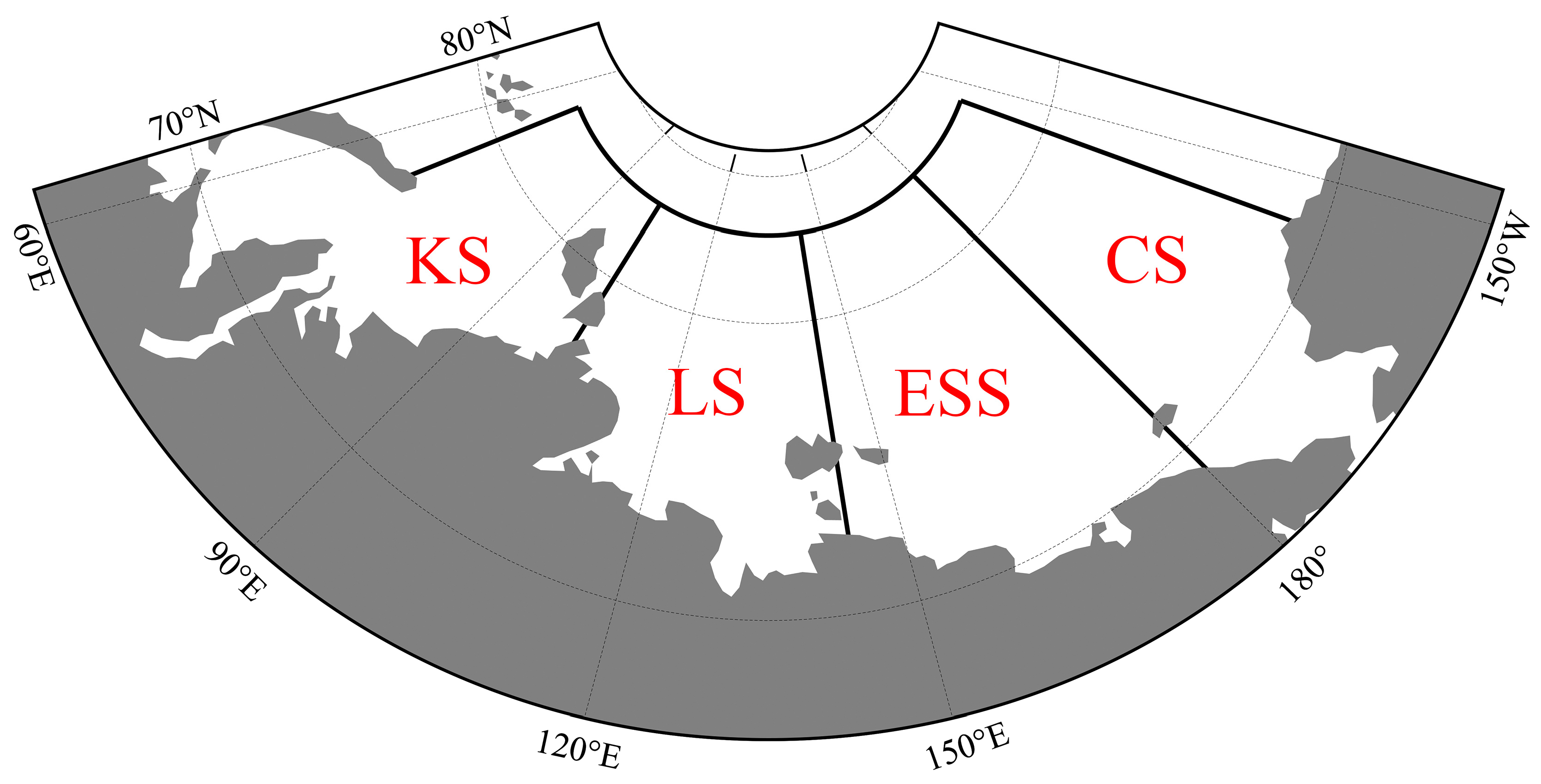
This section first introduces the study area and describes the required datasets and the methods used to acquire them. Then, the navigability assessment approach of sea ice parameters is presented. Subsequently, machine learning algorithms are introduced, with detailed explanations of the model training, testing, and validation procedures. Finally, four appropriate evaluation metrics are proposed to assess the classification performance of all the models.

2.1. Study Area

The NEP is a critical Arctic maritime corridor that stretches along the Eurasian coastline from the Barents Sea (BS) to the Bering Strait. It traverses several marginal seas of the Arctic Ocean, including the Kara Sea (KS), Laptev Sea (LS), East Siberian Sea (ESS), and Chukchi Sea (CS). In recent decades, the accelerated retreat of sea ice driven by climate change has significantly enhanced the seasonal accessibility of this route, Vessels with a high ice-class can operate safely even in heavy ice conditions, but for vessels with a low ice-class or no ice-class, such as Polar Class (PC) 6, PC7, and Open Water (OW) vessels (PC7 classified as OW in this study), navigating through the NEP remains a formidable challenge even during the warm season. Given the Arctic’s complex and dynamic ice conditions, accurate navigability assessments are essential for identifying safe and efficient shipping routes. This underscores the importance of developing and evaluating models capable of effective risk identification and navigational decision-making.

This study focuses on the four key sea areas along the NEP: KS, LS, ESS, and CS. Although the BS is geographically part of the NEP, it is excluded from this study due to its persistent ice-free condition during summer months, largely influenced by the warm inflow of the North Atlantic Current [23]. Figure 1 illustrates the four sea areas classified according to the boundary criteria defined by the National Snow and Ice Data Center (NSIDC) [24].

2.2. Data Preparation

The Navigation Risk Assessment models employ a binary classification framework (see

Table 1. Binary classification confusion matrix.

	Projected Positive Sample	Projected Negative Sample
Actual positive sample	True positive (TP)	False negative (FN)
Actual negative sample	False positive (FP)	True negative (TN)

) to assess vessel navigability and classify the vessel’s positions as either navigable or non-navigable based on ice conditions. Accordingly, the first step of this study involves collecting positive samples (navigable positions) and negative samples (non-navigable positions) to enable subsequent work.

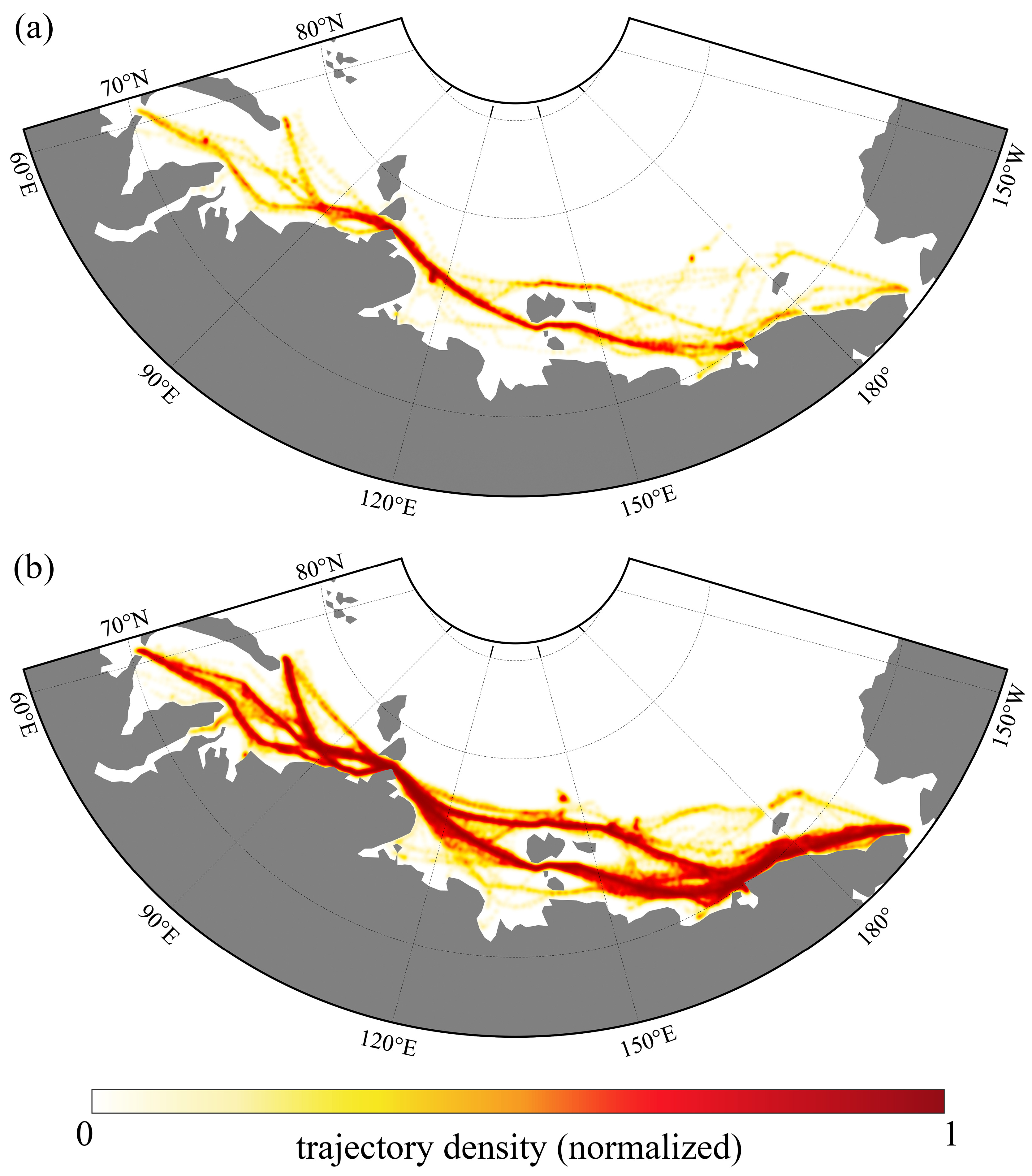
2.2.1. Positive Sample

This study used the position information of trajectory points provided by AIS as the source of positive sample data. AIS data enable global ship monitoring by receiving ship signals from any position in the world, including the polar region and open ocean areas. The rich data provided by the AIS are being increasingly applied in Arctic maritime research to analyze the activities of vessels in the area [25,26]. The position information recorded by AIS is the real-time data of vessels, which can be used to prove that the position was navigable at that time, but it can not indicate that there was no navigation risk. In order to eliminate the data in the AIS records that were navigable but with relatively high navigation risks, this paper referred to the vessel’s speed data recorded in AIS data. The absence of obvious speed reduction data can prove that the data used had a relatively high possibility of safe navigation.

AIS data are derived from ocean-going ship navigation data acquired by the HY-1C/D satellite and distributed by the China Ocean Satellite Data and Distribution System (OSDDS). The dataset covers the period from July to November for each year between 2019 and 2023. During preprocessing, only vessels that successfully navigated through the NEP were considered. AIS records were first grouped by vessels’ MMSI to reconstruct individual voyages. Then, records that fell outside the study area, had missing coordinates, and had excessive time intervals were removed, along with duplicate entries identified by timestamp and coordinates. After cleaning, 8599 trajectory points of PC6 ships and 42,409 trajectory points of OW ships were obtained. Figure 2 shows the trajectory distribution of these positive samples in the four sea areas along the NEP. AIS data are real navigation data. When PC6 and OW vessels navigate through the NEP, they not only consider the impact of sea ice conditions but also tend to follow historical routes, resulting in aggregation as shown in Figure 2. The regional generalization ability of AIS data is weak.

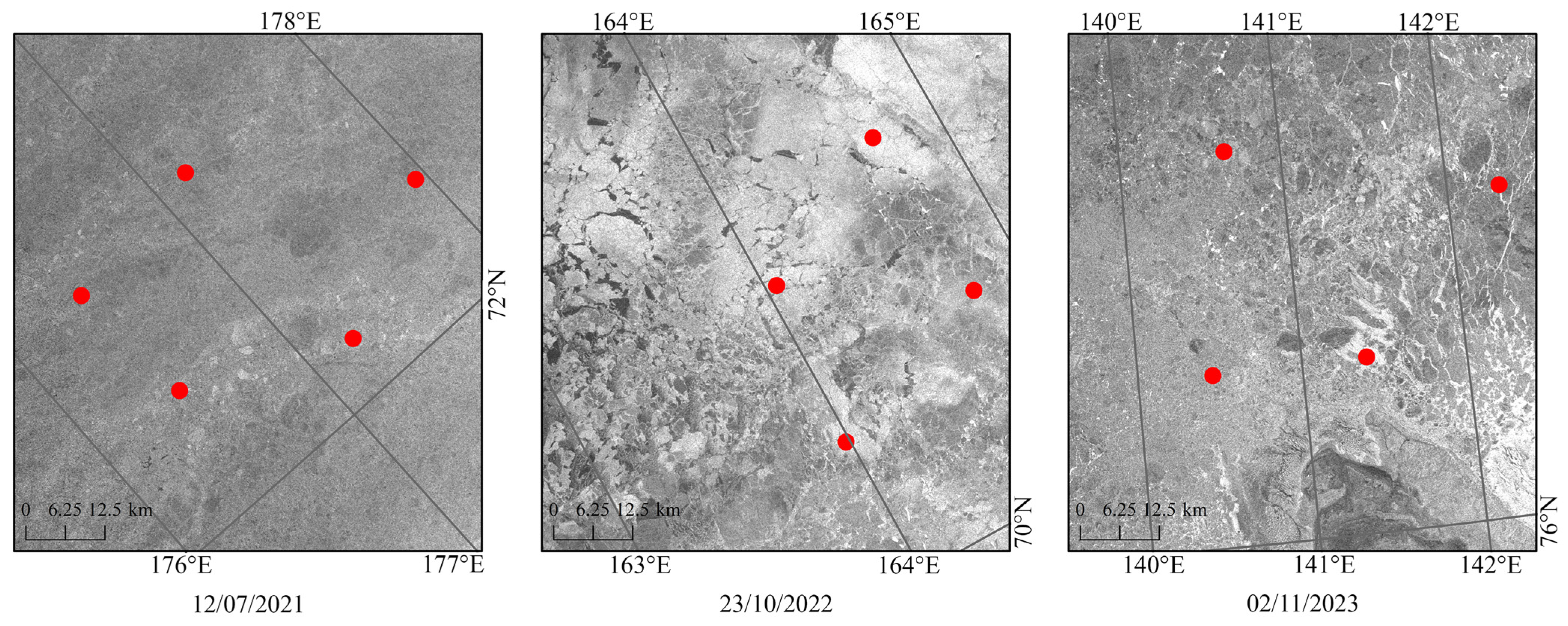
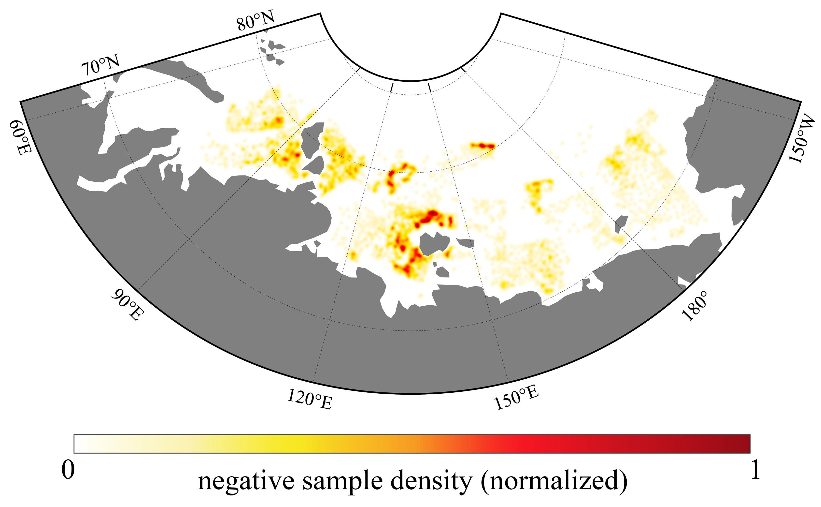
2.2.2. Negative Sample

Due to the lack of negative samples (i.e., non-navigable positions) in AIS trajectory data, this study introduced additional data derived from multi-temporal radar imagery acquired by the Sentinel-1 satellite, which provides high-resolution Synthetic Aperture Radar (SAR) observations of the Arctic. Sentinel-1 is particularly well-suited for sea ice monitoring because it operates in the C-band and offers all-weather, day-and-night imaging capabilities. Its high spatial resolution and sensitivity to surface roughness and dielectric properties enable the effective identification of severe ice conditions, including densely packed multi-year ice and consolidated ice regions that are impassable to low ice-class vessels.

The Sentinel-1 SAR images used in this study were obtained from the Alaska Satellite Facility Distributed Active Archive Center, and all images were acquired within the time range covered by the AIS dataset used in this study. These images also involve regions not recorded by AIS along the NEP, as such areas may be affected by more severe ice conditions that prevent vessels from entering. According to the existing Navigation Risk Assessment Models based on sea ice parameters [15,16,17,18,19,20], PC6 and OW vessels face high risks when navigating in areas with 100% SIC, making such areas unsuitable for navigation. Therefore, the criteria for selecting negative samples in this study are as follows: first, the regions chosen for negative samples should be as close as possible to the AIS data areas of the same day and covered by sea ice on a large scale; second, the entire area within a 6.25 km radius around the selected sample points must be covered by sea ice. By visually interpreting high-resolution SAR imagery, as shown in Figure 3, 2893 representative non-navigable positions were identified and used as negative samples in this study. The latitude and longitude coordinates of these positions were then extracted, and finally, a reliable negative sample set was successfully constructed. Figure 4 shows the trajectory density of these negative samples in the four sea areas of NEP.

2.2.3. Sea Ice Parameters

Two key sea ice parameters, SIC and SIT, were used in this study. The SIC data are sourced from the University of Bremen’s Advanced Microwave Scanning Radiometer 2 (AMSR2) product, which provides daily observations at a spatial resolution of 6.25 km since 2 July 2012. This dataset was processed using the ARTIST Sea Ice (ASI) algorithm [27], effectively reducing atmospheric interference from cloud cover and polar darkness through its 89 GHz channel signature, enabling an accurate characterization of marginal ice regions.

Accurate SIT data are difficult to obtain during the summer months due to the limitations of the satellite sensors. Therefore, a reanalysis SIT dataset with a spatial resolution of 1 degree from the Pan-Arctic Ice Ocean Modeling and Assimilation System (PIOMAS) was selected in this study. The PIOMAS provides long-term estimates of key Arctic cryosphere variables, including SIT, from 1978 to present; it has been widely validated against observed sea ice thickness data [28] and demonstrates the ability to assimilate summer SIT. The dataset was reprojected into the azimuthal equal-area coordinate system (aligned with the SIC) through nearest-neighbor interpolation.

The temporal coverage of SIC and SIT data is the same as that of the AIS dataset, from July to November for each year between 2019 and 2023.

2.3. Methods

2.3.1. Navigability Assessment Approaches of Sea Ice Parameter Models

Table 2. Navigation Risk Assessment Models based on sea ice parameters, including sea ice thickness (SIT) and sea ice concentration (SIC).

No.	References	Sea Ice Parameters	Models	Explanation
1	(Transport Canada, 2018) [15]	SIT	$SIT\le 0.15 \mathrm{m}$ for Open Water (OW) $SIT\le 1.2 \mathrm{m}$ for Polar Class (PC) 6	OW and PC6 vessels can safely navigate when the maximum SIT along the route does not exceed 0.15 m and 1.2 m, respectively.
2	(Lei et al., 2015) [16]	SIC	$SIC\le 50\%$ for PC6	PC6 vessels can safely navigate when the maximum SIC along the route does not exceed 50%.
3	(Khon et al., 2010) [17]	SIC	$SIC\le 15\%$ for OW	OW vessels can safely navigate when the maximum SIC along the route does not exceed 15%.
4	(Shibata et al., 2013) [18]	SIC	$SIC\le 30\%$ for OW	OW vessels can safely navigate when the maximum SIC along the route does not exceed 30%.
5	(Ji et al., 2021) [19]	SIC	$SIC\le 40\%$ for OW	OW vessels can safely navigate when the maximum SIC along the route does not exceed 40%.
6	(Transport Canada, 2018) [15]	SIC, SIT	Arctic Transport Accessibility Model (ATAM) with the equation: $IN=\left(C_1\times I{M}_1\right)+\left(C_2\times I{M}_2\right)$$+I+(C_n\ast I{M}_n)$	OW and PC6 vessels can safely navigate when the $IN$ value along the route is not less than 0.
7	(IMO, 2016) [20]	SIC, SIT	Polar Operational Limit Assessment Risk Indexing System (POLARIS) with the equation: $RIO=\left(C_1\times RI{V}_1\right)+\left(C_2\times RI{V}_2\right)$$+I +(C_n\times RI{V}_n)$	OW and PC6 vessels can safely navigate when the $RIO$ value along the route is not less than 0.

lists seven single or dual sea ice parameter models evaluated in this study: (1) five single sea ice parameter models, and (2) two dual sea ice parameter models (ATAM and POLARIS). The following describes the navigability assessment methods of these models.

For each positive and negative sample, the corresponding date and coordinate information were extracted, and the coordinate information was mapped onto the SIC data grid system to identify the corresponding georeferenced grid cells. Daily SIC and SIT datasets were then used to retrieve ice conditions matched to the date and position of each trajectory point. This approach ensures that each sample position is accurately matched with the surrounding sea ice conditions on the same day, which contributes to a more precise evaluation of models’ capability in identifying ice conditions and navigation.

For the single sea ice parameter models, navigability can be assessed using the following equation:

$$\left(P_{\left(x,y\right)}⩽T\right)$$

(1)

where $P_{(x,y)}$ is the SIC or SIT value within a specific grid cell along the route; and $T$ denotes the designated SIC or SIT threshold, which defines the upper limit of sea ice conditions permissible for safe navigation. If the SIC or SIT values at all positions recorded by AIS along the route are below the threshold, the voyage is classified as navigable by the model. Otherwise, the voyage is classified as non-navigable.

For the dual sea ice parameters models, referring to [15], the navigability assessment approach of the ATAM is as follows:

$$IN=Ca\times IMa+Cb\times IMb+\cdots +Cn\times IMn$$

(2)

where $Ca$, $Cb$, …, $Cn$ represent the sea ice concentrations of different ice types; and $IMa$, $IMb$, …, $IMn$ are the ice multipliers of ice types a, b, and n, respectively. The $IM$ value is an integer ranging from −4 to 2, representing the level of navigational risk posed by a specific ice type to a given ice-class vessel, and higher $IM$ values indicate a lower risk. If $IN$ is negative, the ice condition within the grid cell is considered highly hazardous and safe navigation is infeasible. A route is classified as navigable only if all positions recorded by the AIS are non-negative IN values; otherwise, it is considered non-navigable.

Similarly, referring to [20], the navigability assessment approach of POLARIS is shown in the following equation:

$$RIO=C_1\times R{V}_1+C_2\times R{V}_2+\cdots +C_n\times R{V}_n$$

(3)

where $C_1$, $C_2$, …, $C_n$ is the concentration of different sea ice type; and $R{V}_1$, $R{V}_2$, …, $R{V}_n$ are the risk index values, which denote the corresponding risk index values assigned to each ice type for a given ice-class vessel, ranging from −6 to 3, and differ from the $IM$ value range but follow the same principle: a higher value indicates a lower risk. The risk index outcome (RIO) is computed for each grid cell, and a route is classified as navigable only if all positions recorded by the AIS are non-negative RIO values; otherwise, it is considered non-navigable.

2.3.2. Construction of Navigation Risk Assessment Models Based on ML

To improve the accuracy of navigability assessment in the Arctic region, this study introduced a series of ML models to construct new Navigation Risk Assessment models based on sea ice parameters. ML has shown significant advantages in classification tasks, as it can automatically learn underlying patterns from large-scale data, adapt to complex and high-dimensional input features, and effectively construct the nonlinear relationships between inputs and outputs, thereby improving classification accuracy. ML has been widely applied in various fields such as medical diagnosis, financial risk control, text processing, and image recognition [29,30,31,32], exhibiting strong performance and broad applicability. In this study, the classification task is considered a binary problem, where each input sample is assigned a label of either 1 (navigable) or 0 (non-navigable). As the sea ice parameter models, the input features used by the ML models are also SIC and SIT, and the output result is 1 (navigable) or 0 (non-navigable). A total of 10 ML models were employed in this study to capture the complex relationships between ice conditions and navigability, including Logistic Regression (LR), K-Nearest Neighbors (KNN), Support Vector Classifier (SVC), Multi-layer Perceptron (MLP), Random Forest (RF), ExtraTrees Classifier (ETC), Gradient Boosting Machine (GBM), Extreme Gradient Boosting (XGBoost), Light Gradient Boosting Machine (LightGBM), and Categorical Boosting (CatBoost).

LR [33] is a linear classification algorithm that estimates the probability of a binary outcome using the logistic (sigmoid) function. It is simple, interpretable, and effective when the relationship between features and output is approximately linear. During binary classification, by default, if the predicted probability exceeds 0.5 by LR, the sample is classified as the positive class; otherwise, it is classified as the negative class.

KNN [34] is a simple, non-parametric algorithm that classifies samples based on the majority label of their K-Nearest Neighbors in feature space. It does not assume any underlying data distribution and works well for datasets with clear local structure. However, KNN is sensitive to the choice of distance metric and can be computationally expensive for large datasets.

SVC [35], based on Support Vector Machines (SVM), seeks to find an optimal separating hyperplane with maximum margin between classes. By using kernel tricks (e.g., RBF, polynomial), it can handle both linear and nonlinear classification problems effectively. SVC is robust in high-dimensional spaces but may require careful tuning of hyperparameters like the regularization parameter and kernel choice.

MLP [36] is a feedforward artificial neural network consisting of an input layer, one or more hidden layers, and an output layer. Each neuron performs a nonlinear transformation using activation functions like ReLU or sigmoid. MLP is trained via backpropagation to minimize prediction error and is capable of modeling complex, nonlinear relationships.

RF [37] is an ensemble learning algorithm that constructs multiple decision trees using random subsets of data and features. It aggregates their outputs to improve predictive accuracy and robustness. RF is less prone to overfitting than a single tree and can handle high-dimensional data effectively. It also provides insights into feature importance, aiding in model interpretation.

ETC [38] is an ensemble method similar to RF but introduces additional randomness by selecting split thresholds completely at random. This results in faster training and often lower variance. ETC works well on noisy or high-dimensional datasets and is less sensitive to parameter tuning than some other tree-based methods.

GBM [39] is a powerful ensemble method that builds trees sequentially, with each tree correcting the errors of its predecessor. It optimizes a loss function using gradient descent, allowing for high accuracy. GBM can construct complex patterns, but it is sensitive to hyperparameters such as learning rate and number of trees, requiring careful tuning.

XGBoost [40] is an optimized gradient boosting library for speed and performance. It incorporates regularization (L1 and L2) to prevent overfitting and supports parallel computation, missing value handling, and sparse data optimization. XGBoost consistently achieves superb results in many classification and regression tasks, especially on structured tabular data.

LightGBM [41] is a gradient boosting framework that uses histogram-based algorithms to accelerate training and reduce memory usage. It grows trees leaf-wise rather than level-wise, improving accuracy. LightGBM is highly efficient on large datasets and handles categorical features directly, making it well-suited for high-speed, high-accuracy machine learning tasks.

CatBoost [42] CatBoost is also a gradient boosting algorithm that can handle categorical features effectively without extensive preprocessing. CatBoost uses ordered boosting to reduce overfitting and provides strong performance out of the box. It is robust to parameter settings, handles missing values naturally, and is often preferred in business applications with many categorical variables.

In this study, a random splitting method was employed to model construction. For PC6 navigable binary classification models training, 2000 samples were randomly selected from 8599 positive samples and 2893 negative samples, respectively. For OW navigable binary classification models training, 2000 samples were randomly selected from 42,409 positive samples, and the negative samples were the same as those used for training the PC6 navigable binary classification models. The two datasets were randomly split into training and testing sets using a 7:3 ratio. The 7:3 ratio is commonly used for splitting training and testing sets in machine learning, as it can better balance the model’s learning ability and performance adjustment [43]. Five-fold cross-validation method is applied during training and hyperparameter tuning to improve model robustness and reduce variance caused by data partitioning.

To discuss the optimal amount of training samples, Figure 5 shows the learning curves of 10 ML models. Among KNN, SVC, RF, ETC, GBM, XGBoost, LightGBM, and CatBoost ML models, the performance of the binary classification models often increases with the number of training samples. When the size reaches about 1200, the learning curves gradually flatten out. Therefore, it is reasonable for this research to adopt 2000 as the number of training samples. However, for LR, SVC, and MLP, little improvement is shown. The efficiency and applicability of these algorithms in this study are questionable, and in Section 3.2 we found that these three models perform poorly.

2.3.3. Evaluation Metrics

Given the class imbalance between positive and negative samples in this study, four commonly used evaluation metrics were adopted: True Positive Rate (TPR), False Positive Rate (FPR), F1-score, and Matthews Correlation Coefficient (MCC), as shown in

Table 3. The formulas and optimal values of the four metrics used in this study.

Metric Name	Formula	Optimum Value
TPR	${\displaystyle \frac{TP }{ \left(TP+FN\right)}}$	1
FPR	${\displaystyle \frac{FP }{ \left(FP+TN\right)}}$	1
F1-score	${\displaystyle \frac{2\times TP}{2\times TP+FP+FN}}$	1
MCC	${\displaystyle \frac{TP\times TN-FP\times FN}{\sqrt{(TP+FP)(TP+FN)(TN+FP)(TN+FN)}}}$	1

. Furthermore, undersampling and oversampling techniques are used to balance the remaining samples, which are not selected for training and testing, to adjust the imbalanced validation samples [44].

TPR is also known as recall or sensitivity. It remains unaffected by class distribution imbalances, as it only considers actual positive samples in its denominator, and measures the proportion of correctly identified positive samples to all actual positive samples [45]. A higher TPR indicates a better ability of the model to detect navigable conditions.

FPR measures the proportion of negative samples that are incorrectly classified as positive among all actual negative samples. In contrast to TPR, FPR focuses solely on the model’s performance in classifying negative samples [44]. A lower FPR implies that the model is less likely to misclassify non-navigable positions as navigable.

F1-score is the harmonic mean of precision and recall, providing a balanced measure between false positives and false negatives. It ensures a fair evaluation of model performance by mitigating biases caused by class imbalance [46].

MCC is a robust and comprehensive metric. It takes into account all four elements of the confusion matrix and returns a value between –1 and 1, where 1 indicates perfect prediction, 0 indicates no better than random prediction, and –1 indicates total disagreement between prediction and observation. MCC provides a more accurate and balanced overall evaluation of classifier performance, particularly in cases of imbalanced sample distributions [47,48]. The MCC values obtained in this study were normalized (nMCC) to facilitate comparison with other evaluation metrics.

The specific evaluation metrics are as follows: firstly, we focus on the TPR. If the TPR is less than 0.9500, it means that over 5% of the navigable positions cannot be detected by this model, indicating that the model has poor applicability in this study. Secondly, we pay attention to the FPR. If the FPR value is greater than 0.0500, it indicates that over 5% of the navigable positions identified by the model actually threaten vessel safety. Finally, we consider both the F1-score and nMCC values. The performance of the model improves as these values increase.

3. Results

This section presents the classification results and evaluation metrics of both the sea ice parameter models and the machine learning models, and analyzes their capability to identify navigable and non-navigable samples for PC6 and OW vessels. Based on these results, the monthly navigability along the Northeast Passage is further assessed using these models, followed by validation of the assessment outcomes. Finally, a sensitivity analysis of the machine learning models is conducted to determine which sea ice parameter has a greater impact on the navigability of PC6 and OW vessels.

3.1. Classification Results of Sea Ice Parameter Models

According to the methodology described in Section 2.3.3, the sea ice parameter models performed the classification task using the same independent prediction set as the machine learning models. Subsequently, after applying undersampling and oversampling techniques to balance the independent validation dataset, the classification results were evaluated using four metrics: TPR, FPR, F1-score, and nMCC. The results are presented in

Table 4. Classification results and evaluation metrics of sea ice parameter models implementing the undersampling technique and the oversampling technique, respectively.

Sampling Technique	Vessel Type	Model	TP	FN	FP	TN	TPR	FPR	F1-Score	nMCC
Under- sampling	PC6	Model 1. $\mathrm{S}\mathrm{I}\mathrm{T}\le 1.2 \mathrm{m}$	889	4	848	45	0.9955	0.9496	0.6760	0.5703
		Model 2. $\mathrm{S}\mathrm{I}\mathrm{C}\le 50\mathrm{\%}$	760	133	10	883	0.8511	0.0112	0.9140	0.9240
		Model 6. ATAM	889	4	850	43	0.9955	0.9518	0.6755	0.5682
		Model 7. POLARIS	889	4	810	83	0.9955	0.9071	0.6860	0.6027
	OW	Model 1. $\mathrm{S}\mathrm{I}\mathrm{T}\le 0.15 \mathrm{m}$	813	80	44	849	0.9104	0.0493	0.9291	0.9309
		Model 3. $\mathrm{S}\mathrm{I}\mathrm{C}\le 15\mathrm{\%}$	746	147	0	893	0.8354	0.0000	0.9103	0.9235
		Model 4. $\mathrm{S}\mathrm{I}\mathrm{C}\le 30\mathrm{\%}$	761	132	2	891	0.8522	0.0022	0.9191	0.9295
		Model 5. $\mathrm{S}\mathrm{I}\mathrm{C}\le 40\mathrm{\%}$	771	122	3	890	0.8634	0.0034	0.9250	0.9339
		Model 6. ATAM	826	67	59	834	0.9250	0.0661	0.9291	0.9295
		Model 7. POLARIS	826	67	52	841	0.9250	0.0582	0.9328	0.9334
Over- sampling	PC6	Model 1. $\mathrm{S}\mathrm{I}\mathrm{T}\le 1.2 \mathrm{m}$	6569	30	6362	237	0.9955	0.9641	0.6727	0.5557
		Model 2. $\mathrm{S}\mathrm{I}\mathrm{C}\le 50\mathrm{\%}$	5541	1058	93	6506	0.8397	0.0141	0.9059	0.9173
		Model 6. ATAM	6569	30	6366	233	0.9955	0.9647	0.6726	0.5550
		Model 7. POLARIS	6569	30	6070	529	0.9955	0.9198	0.6829	0.5939
	OW	Model 1. $\mathrm{S}\mathrm{I}\mathrm{T}\le 0.15 \mathrm{m}$	36,935	3484	1337	39,072	0.9138	0.0331	0.9387	0.9410
		Model 3. $\mathrm{S}\mathrm{I}\mathrm{C}\le 15\mathrm{\%}$	33,616	6803	0	40,409	0.8317	0.0000	0.9081	0.9219
		Model 4. $\mathrm{S}\mathrm{I}\mathrm{C}\le 30\mathrm{\%}$	34,383	6036	61	40,348	0.8507	0.0015	0.9186	0.9293
		Model 5. $\mathrm{S}\mathrm{I}\mathrm{C}\le 40\mathrm{\%}$	34,560	5859	137	40,272	0.8550	0.0034	0.9202	0.9302
		Model 6. ATAM	37,454	2965	2300	38,109	0.9266	0.0569	0.9343	0.9349
		Model 7. POLARIS	37,468	2951	1967	38,442	0.9270	0.0487	0.9384	0.9393

.

Table 4 reveals notable differences in classification performance between the models. For PC6 vessels, both under the scenarios of undersampling and oversampling, Model 1, Model 6 (ATAM), and Model 7 (POLARIS) achieved near-perfect TPR results, but the FPR values can reach 0.9000. This indicates that these models are capable of correctly identifying the vast majority of navigable samples; however, their extremely high FPR results suggest a substantial overestimation of the vessels’ operational capability under given ice conditions, and they can barely identify the non-navigable positions. In practical navigation scenarios, these models could lead to misclassification of non-navigable areas as navigable, posing significant operational risks. Model 2, which relies solely on the SIC threshold, achieved moderate TPR values (0.8511 and 0.8397) and excellent FPR values (0.0112 and 0.0141), indicating relatively best performance. Therefore, for PC6 vessels, Model 2 has the best navigation strategy.

For OW vessels, both under the scenarios of undersampling and oversampling, Model 1, Model 6 (ATAM), and Model 7 (POLARIS) showed slightly unsatisfied TPR values (0.9104–0.9270) and FPR values (0.0331–0.0661). The divergences between the three models are small, the maximum difference between F1-score is 0.004, and the maximum difference in nMCC is 0.0061. These three models reveal a tendency to underestimate navigability in ice regions and adopt a more cautious navigation strategy. Models 3, 4, and 5, which rely solely on the SIC thresholds (15%, 30%, and 40%, respectively), achieved exceptionally low FPRs, and Model 3 does not even make an error in classifying the negative samples, showing strong ability in identifying negative samples. However, this came at the cost of sensitivity, as evidenced by their high FN values, especially in Model 3, which had the highest number of misclassified positive samples. Therefore, these models show an obvious drop in TPR results, indicating that they are more likely to make errors when identifying navigable conditions. Correspondingly, their F1-score and nMCC results also showed a downward trend. These models tend to adopt conservative classification strategies and underestimate navigable opportunities, and may not be a good choice to use them for practical applications because they will reduce shipping efficiency.

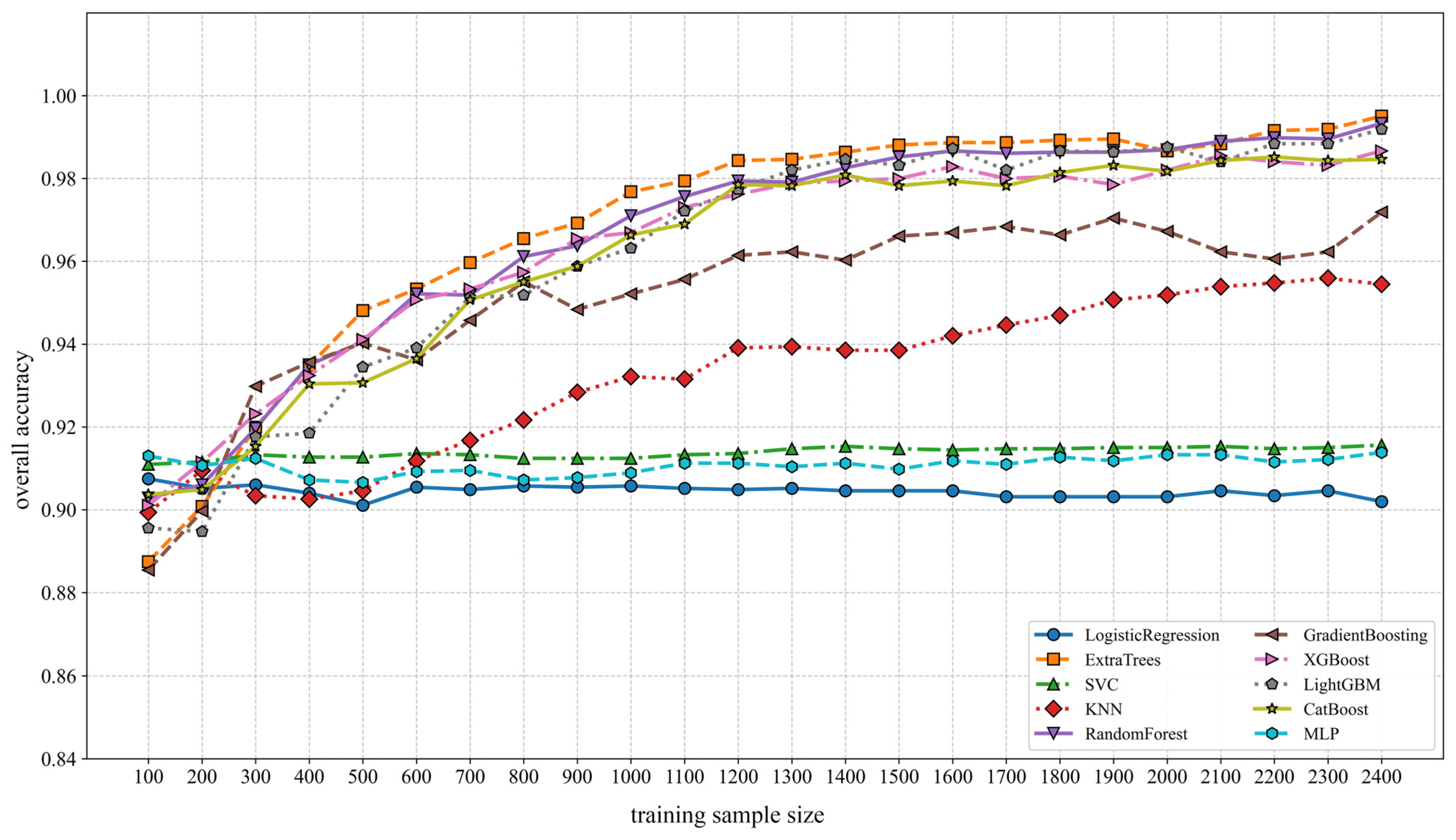
3.2. Classification Results of Machine Learning Models

The evaluation of sea ice parameter models reveals that they cannot accurately distinguish between navigable and non-navigable conditions, and are unable to balance navigational safety and transport efficiency. To address these limitations, ML models were introduced to enhance the accuracy of sea ice risk identification. This section evaluates and compares the classification performance of 10 ML models based on the independent prediction set.

Table 5. Classification results and evaluation metrics of ML models for PC6 vessel implementing the undersampling technique and the oversampling technique, respectively.

Sampling Technique	Model	TP	FN	FP	TN	TPR	FPR	F1-Score	nMCC
Under- sampling	ETC	892	1	7	886	0.9989	0.0078	0.9955	0.9955
	RF	892	1	6	887	0.9989	0.0067	0.9961	0.9961
	XGBoost	887	6	14	879	0.9933	0.0157	0.9888	0.9888
	LightGBM	891	2	17	876	0.9978	0.0190	0.9894	0.9894
	CatBoost	879	14	12	881	0.9843	0.0134	0.9854	0.9854
	GBM	886	7	9	884	0.9922	0.0101	0.9910	0.9910
	KNN	865	28	62	831	0.9686	0.0694	0.9496	0.9499
	MLP	812	81	24	869	0.9093	0.0269	0.9412	0.9421
	LR	772	121	28	865	0.8645	0.0314	0.9166	0.9189
	SVC	809	84	18	875	0.9059	0.0202	0.9429	0.9441
Over- sampling	ETC	6596	3	46	6553	0.9995	0.0070	0.9963	0.9963
	RF	6596	3	52	6547	0.9995	0.0079	0.9958	0.9958
	XGBoost	6559	40	111	6488	0.9939	0.0168	0.9886	0.9886
	LightGBM	6581	18	122	6477	0.9973	0.0185	0.9894	0.9895
	CatBoost	6515	84	75	6524	0.9873	0.0114	0.9880	0.9880
	GBM	6554	45	76	6523	0.9932	0.0115	0.9908	0.9908
	KNN	6411	188	491	6108	0.9715	0.0744	0.9486	0.9490
	MLP	5925	674	90	6509	0.8979	0.0136	0.9421	0.9439
	LR	5648	951	191	6408	0.8559	0.0289	0.9135	0.9162
	SVC	5905	694	52	6547	0.8948	0.0079	0.9435	0.9456

and

Table 6. Classification results and evaluation metrics of ML models for OW vessel implementing the undersampling technique and the oversampling technique, respectively.

Sampling Technique	Model	TP	FN	FP	TN	TPR	FPR	F1-Score	nMCC
Under- sampling	ETC	856	37	10	883	0.9586	0.0112	0.9733	0.9739
	RF	853	40	18	875	0.9552	0.0202	0.9671	0.9677
	XGBoost	824	69	7	886	0.9227	0.0078	0.9559	0.9586
	LightGBM	835	58	6	887	0.9351	0.0067	0.9631	0.9650
	CatBoost	826	67	8	885	0.9250	0.0090	0.9566	0.9590
	GBM	831	62	9	884	0.9306	0.0101	0.9590	0.9611
	KNN	811	82	14	879	0.9082	0.0157	0.9441	0.9475
	MLP	817	76	22	871	0.9149	0.0246	0.9434	0.9459
	LR	808	85	24	869	0.9048	0.0269	0.9368	0.9400
	ETC	809	84	22	871	0.9059	0.0246	0.9385	0.9417
Over- sampling	ETC	38,561	1848	527	39,882	0.9543	0.0130	0.9701	0.9709
	RF	38,602	1807	931	39,478	0.9553	0.0230	0.9658	0.9662
	XGBoost	37,429	2980	531	39,878	0.9263	0.0131	0.9552	0.9574
	LightGBM	38,012	2397	540	39,869	0.9407	0.0134	0.9628	0.9641
	CatBoost	37,388	3021	401	40,008	0.9252	0.0099	0.9562	0.9586
	GBM	37,666	2743	489	39,920	0.9321	0.0121	0.9589	0.9607
	KNN	36,794	3615	587	39,822	0.9105	0.0145	0.9460	0.9493
	MLP	37,065	3344	762	39,647	0.9172	0.0189	0.9475	0.9501
	LR	36,300	4109	937	39,472	0.8983	0.0232	0.9350	0.9389
	ETC	36,786	3623	349	40,060	0.9103	0.0086	0.9488	0.9523

present the classification results and evaluation metrics of ML models for classifying PC6 and OW vessels implementing the undersampling technique and the oversampling technique, respectively.

For PC6 vessels, it is evident that ensemble learning models (RF, ETC, GBM, XGBoost, LightGBM, and CatBoost) consistently outperform the other four classifiers (LR, KNN, SVC, and MLP) across both vessel types. ETC and RF achieved near-perfect classification results. Their TPR reached 0.9989 and FPR decreased to 0.0079, F1-score results exceeded 0.9900, and nMCC results approached 0.9970. These two models maintained extremely high TPR and low FPR results, indicating that they have an excellent ability to identify both navigable and non-navigable conditions, and their overall classification performance significantly surpasses that of the sea ice parameter models. XGBoost, LightGBM, CatBoost, and GBM also showed strong performance, suggesting that their ability to identify both navigable and non-navigable conditions can still be regarded as excellent, and they are more effective than sea ice parameter models in identifying the risk level when PC6 vessels encounter sea ice.

While ensemble models achieve superior performance, traditional models still produce high metrics and may be suitable in certain contexts. They exhibited increased errors during classification and failed to accurately identify positive samples or negative samples. Consequently, their TPR, F1-score, and nMCC declined, while the FPR rose. Among the 10 models, LR produced the worst classification result for positive samples, achieving the lowest TPR (0.8645 with undersampling and 0.8559 with oversampling).

For OW ships, the evaluation metrics indicated that ensemble learning models still have significant advantages in the task, though variations exist among different models. Among the 10 models, ETC and RF exhibited the strongest performance in terms of TPR and FPR. Their TPR results reached 0.9543–0.9586 and 0.9552–0.9553. Moreover, FPR decreased to 0.0112–0.0130 and 0.0202–0.0230, respectively. Compared to Model 7 (POLARIS)—a superior model among sea ice parameter models—ETC and RF showed a significant improvement in distinguishing between navigable and non-navigable samples. This confirms that decision tree-based Bagging algorithms maintain strong robustness when processing OW vessels data. XGBoost, LightGBM, CatBoost, and GBM also performed well. Compared to the sea ice parameter models, these models are more balanced and show good classification stability across all metrics. They achieved higher or comparable TPR results and significantly reduced FPR results, indicating fewer false predictions of non-navigable conditions under hazardous scenarios. This highlights the ability of the six ML models above to effectively address the misclassification problem commonly seen in sea ice parameter models. The other four models, LP, KNN, MLP, and SVC, lag behind the six ensemble learning models mentioned above. Their classification ability for both positive and negative samples was insufficient. Compared to the sea ice parameter models, they did not show any notable advantage, with several evaluation metrics even falling behind those of the POLARIS. Therefore, these four models are not suitable for navigation risk assessment.

3.3. Further Validation of the Effectiveness of ML Models in Navigability Assessment

To further validate the effectiveness of ML models in navigability assessment, in this section, the optimal sea ice parameter model (POLARIS) and ML model (RF) were selected for comparison based on the comprehensive evaluation metrics in Section 2.3.3. Firstly, daily SIC and SIT values of each grid cell along the NEP were extracted from the SIC latitude–longitude grid data. Then, the navigability of each grid cell was assessed using the POLARIS and the RF separately, based on daily ice conditions. The output was assigned a value of 1 if the grid cell was navigable on that day and 0 if not. Finally, the daily navigability results of each grid cell were aggregated to obtain the monthly number of navigable days along the NEP from July to November for each year during 2019–2023, as shown in Figure 6 and Figure 7, and darker blue colors indicate more navigable days at the grid location, while darker red colors indicate fewer navigable days.

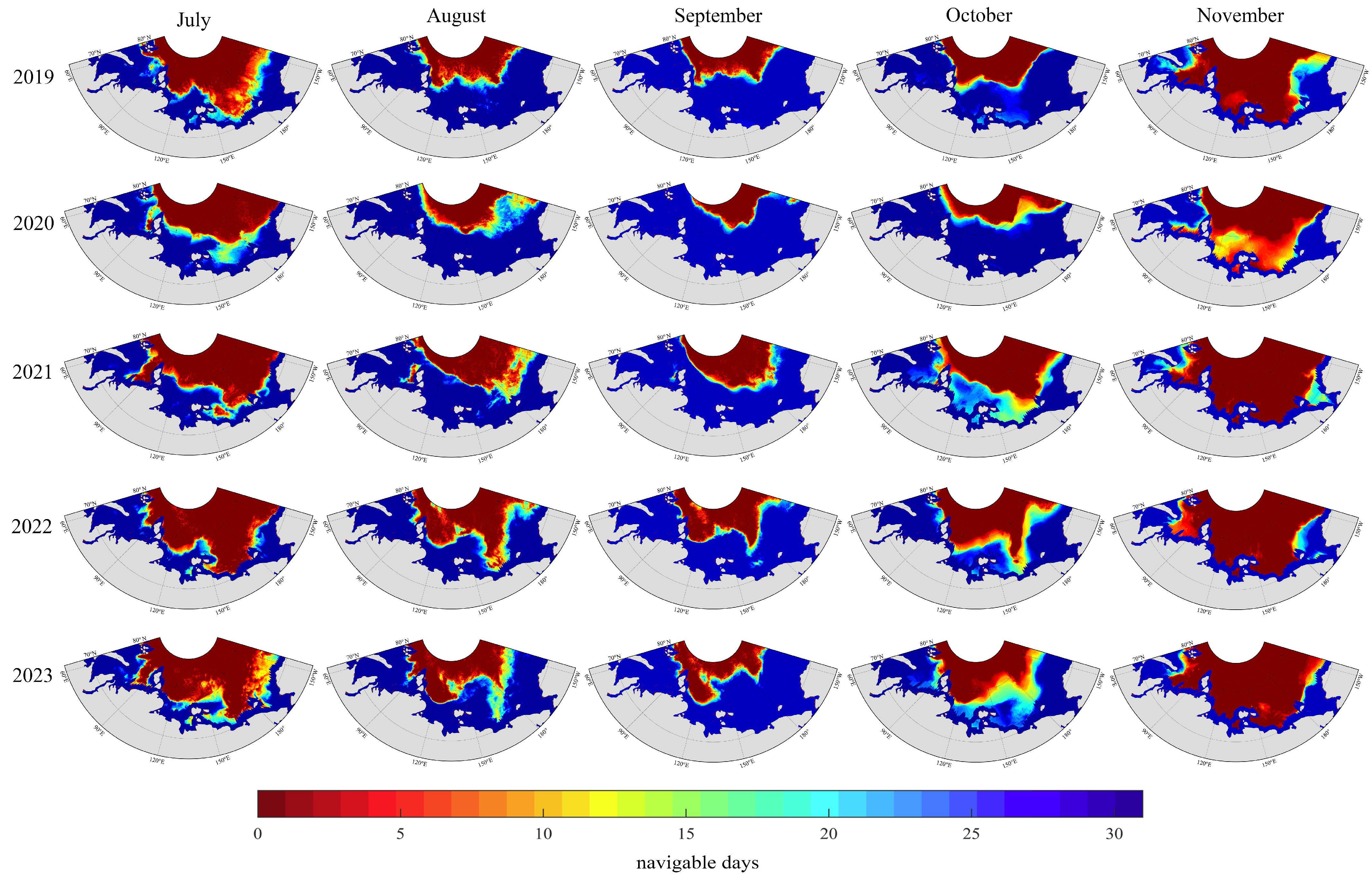
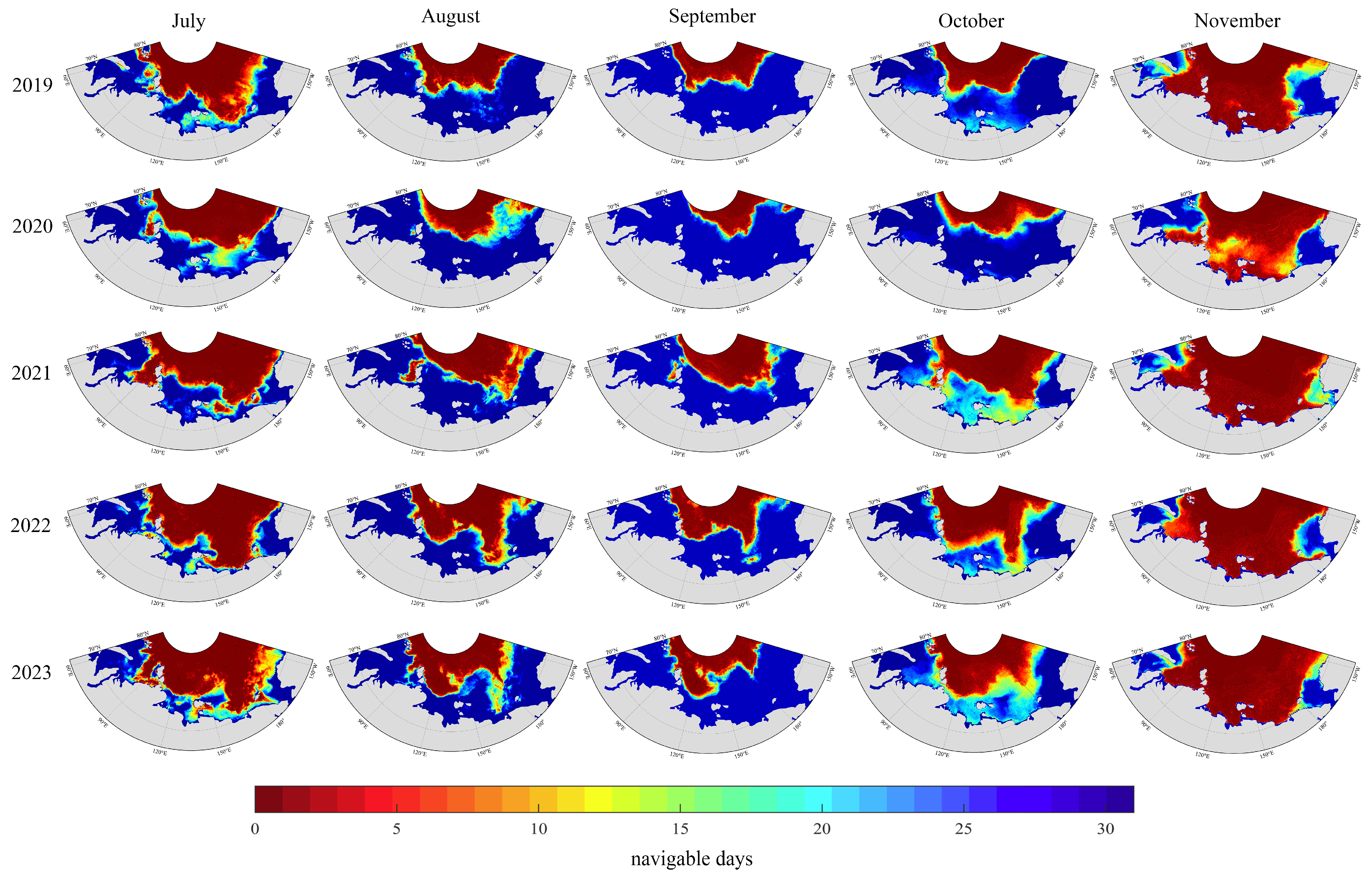
3.3.1. Monthly Navigability of NEP

From the monthly navigability distribution maps assessed using the POLARIS and the RF, despite the differences in navigability results between the two models along the NEP, both consistently indicate that 2020 was the most navigable year along the NEP, September was the most favorable month for OW vessel navigation during the shipping season each year, whereas November exhibited the poorest navigability. In July, the ESS had the worst navigability, and the Vilkitsky Strait also showed notable restrictions, especially in 2021 and 2023. By August, navigability improved significantly along the entire route, but the lower-latitude regions of the ESS still showed worse navigability compared to other sea areas in 2022 and 2023. In September, all maritime regions became fully navigable, achieving complete accessibility throughout the month. In October, navigability declined again, with this decline being especially pronounced in the Vilkitsky Strait and the ESS between 2021 and 2023. In November, due to severe ice conditions, navigation became difficult across the NEP except for the Chukchi Sea, and only in 2020 was there a limited degree of navigability observed.

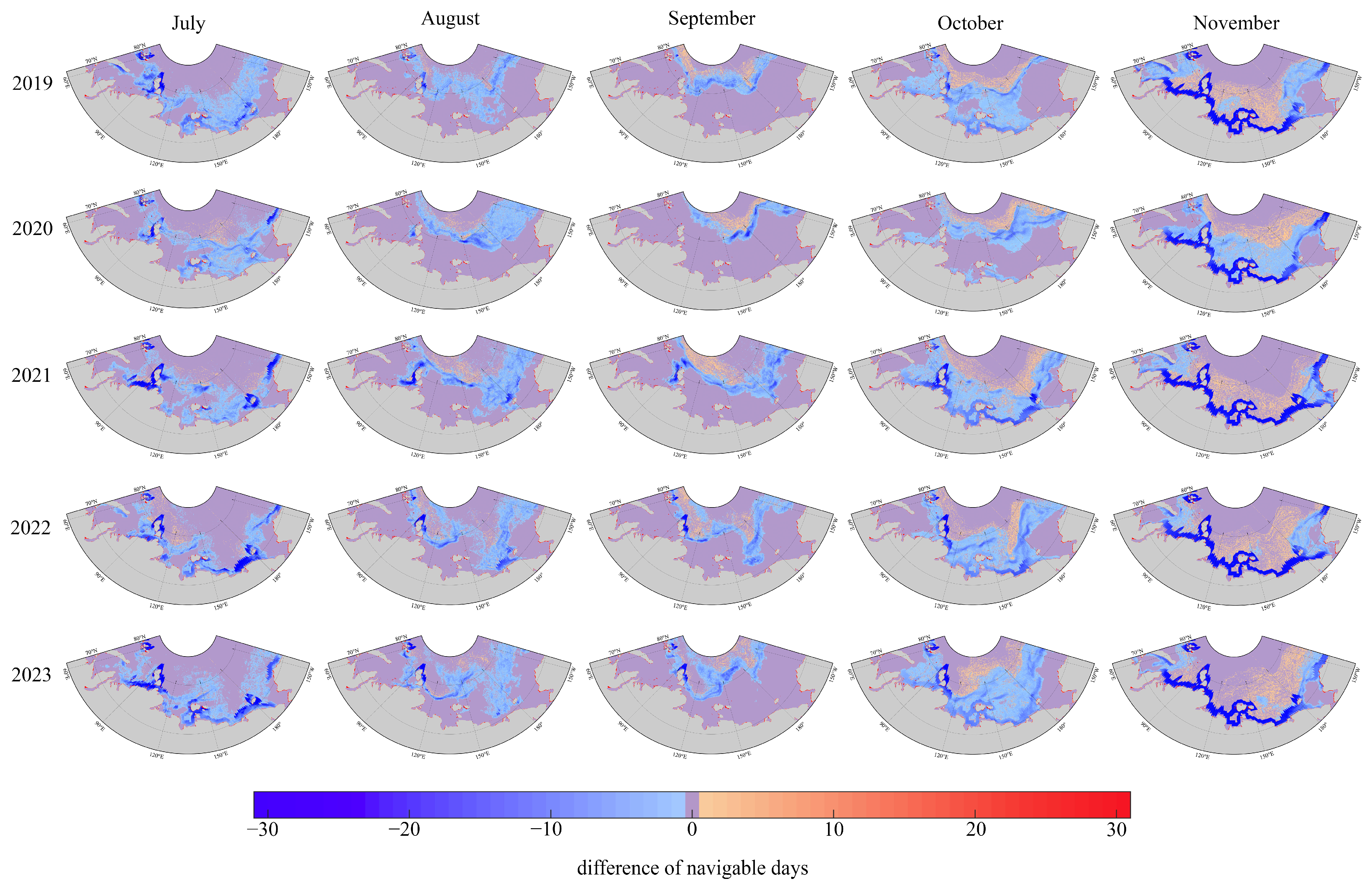
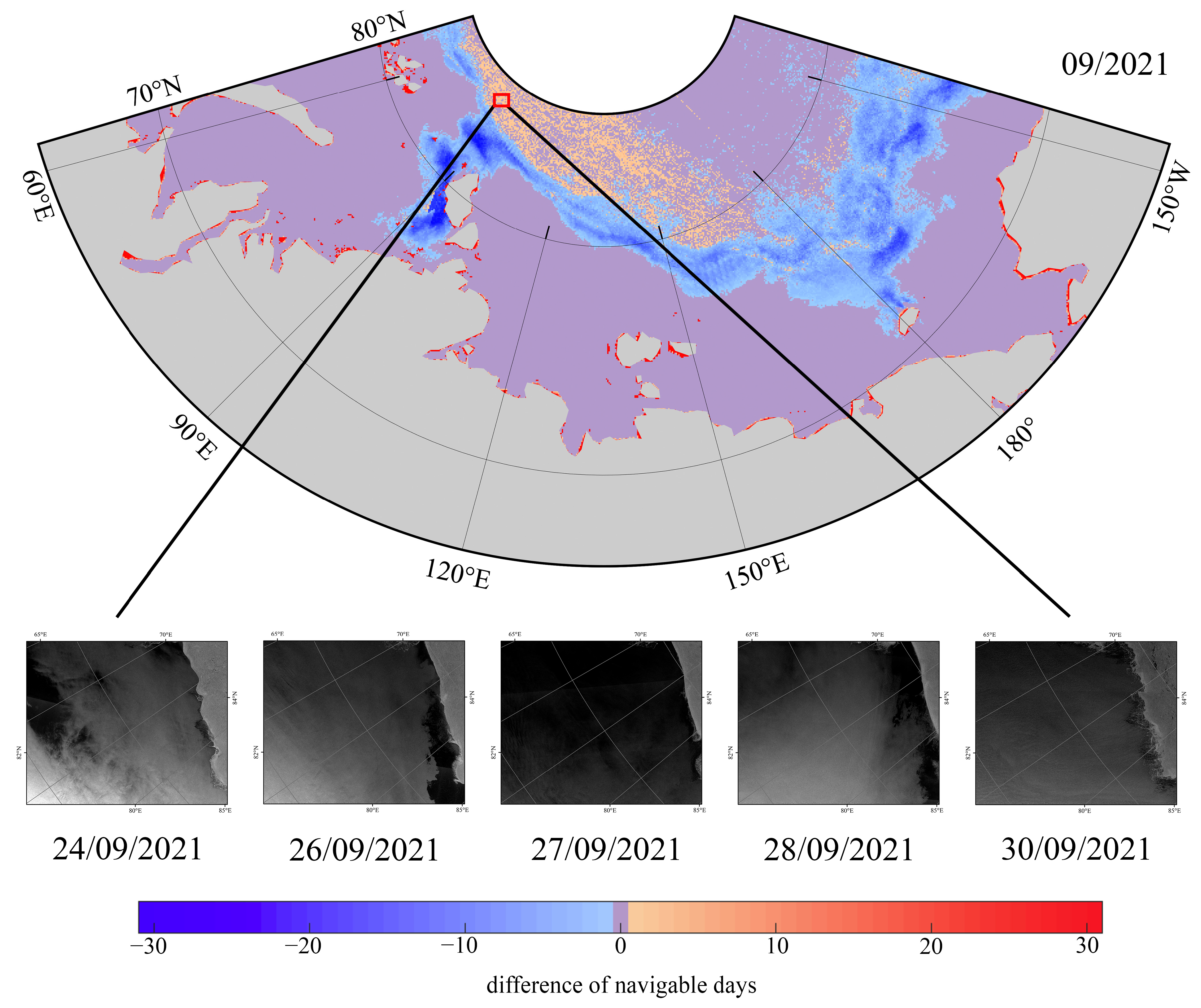
3.3.2. Difference of Monthly Navigability Assessment Results Between POLARIS and RF

To more clearly observe the differences in navigability assessment results between the POLARIS and RF, the two models’ monthly navigability results based on the grid were subtracted, and the resulting differences were visualized. Figure 8 illustrates the spatial distribution of monthly navigability differences along the NEP. Negative values indicate that the monthly number of navigable days assessed with the POLARIS at a grid position is greater than that assessed with the RF, and the closer the color is to blue, the larger the difference. Positive values indicate that the RF predicted more navigable days than the POLARIS at a grid position, and the closer the color is to red, the larger the difference. Purple areas represent grid cells where both models produced the same result, i.e., the difference in navigable days is 0.

It can be seen that the largest differences in monthly navigability assessments between the POLARIS and RF occurred in October and November each year, which was reflected in the area of the regions showing disagreement between the two models. July ranked next, while the differences area in August and September was considerably reduced due to the generally favorable navigability along the NEP during the 2 months. Compared to the POLARIS, RF often produced more optimistic navigability assessments for higher-latitude regions along the same longitude, and this tendency became more pronounced as the navigation season progressed, reaching its largest in November. In contrast, the POLARIS tended to produce better navigability assessment results than RF in lower-latitude areas along the same longitude. To verify the accuracy of models, this study used the monthly navigability difference map for September 2021 and selected a specific position, as shown in Figure 9. At this position, RF indicated the presence of navigable days during the month, while the POLARIS assessed the position as completely non-navigable in this month, which can also be observed in Figure 6 and Figure 7. Based on this discrepancy, Sentinel-1 imagery for the corresponding month and position was retrieved, and visual interpretation confirmed the presence of navigable conditions on multiple days. Figure 7 shows that favorable ice conditions were observed on the 24th, 26th, 27th, 28th, and 30th, and OW vessels can safely traverse this position. This finding confirmed that, compared to the POLARIS, the RF is more accurate in identifying sea ice hazards and is better suited for evaluating the navigability of vessels in ice-covered regions.

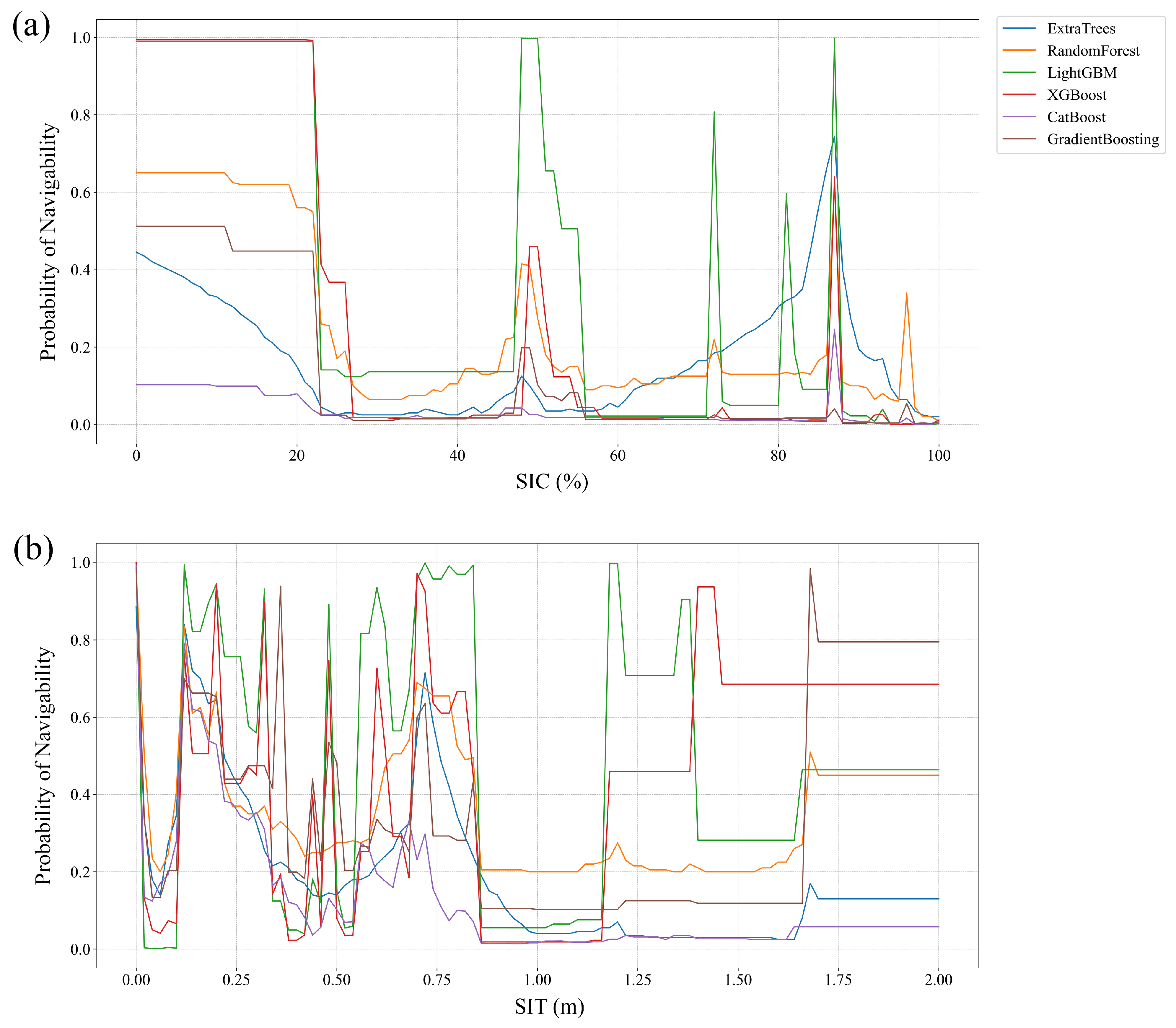
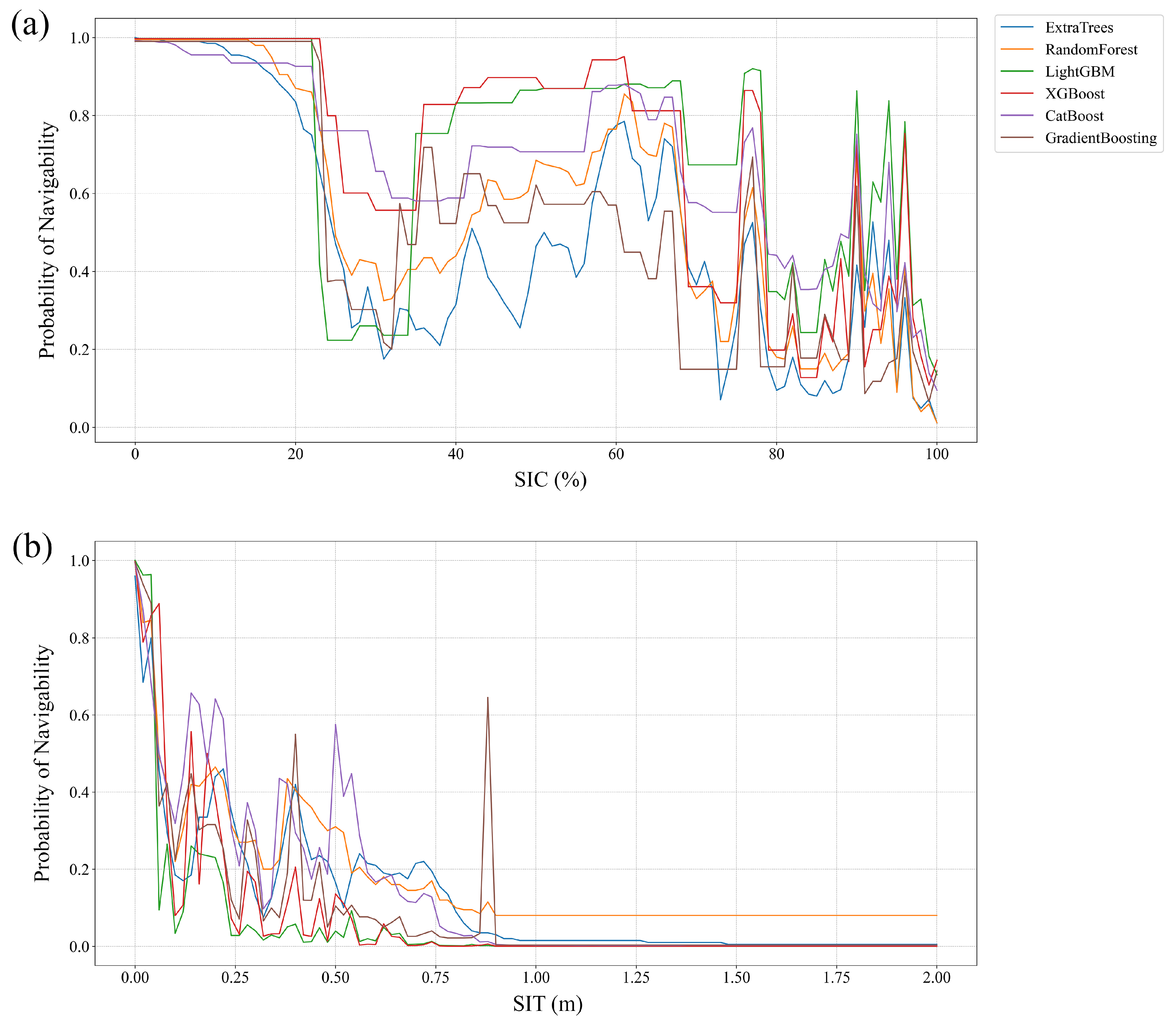
3.3.3. Sensitivity Analysis of ML Models

In this section, the method of single-factor sensitivity analysis was conducted to analyze the sensitivity of affecting the navigability of SIC and SIT. The SIC range was from 0 to 100%, and the SIT range was from 0 to 2 m. Figure 10 and Figure 11, as well as

Table 7. Sensitivity analysis results of SIC and SIT.

Vessel Type	Model	SIC Sensitivity	SIT Sensitivity	More Sensitive Feature
PC6	ETC	0.725	0.86	SIT
	RF	0.64	0.79	SIT
	XGBoost	0.9937	0.98	SIC
	LightGBM	0.9969	0.9989	SIT
	CatBoost	0.2452	0.9795	SIT
	GBM	0.5097	0.8824	SIT
OW	ETC	0.9889	0.955	SIC
	RF	0.9835	0.915	SIC
	XGBoost	0.8887	0.9972	SIT
	LightGBM	0.8627	0.9997	SIT
	CatBoost	0.8972	0.9937	SIT
	GBM	0.9246	0.992	SIT

, illustrate the results.

For PC6 vessels, five of the six models indicated that navigability was more sensitive to changes in SIT than in SIC, with only the result of XGBoost showing greater sensitivity to SIC. In the case of OW vessels, while navigability was found to be highly sensitive to both SIC and SIT, the results from XGBoost, LightGBM, CatBoost, and GBM suggested a higher sensitivity to SIT, and only ETC and RF showed greater sensitivity to SIC. Overall, the majority of models suggest that SIT has a stronger influence on vessel navigability for both PC6 and OW vessels. The results of the sensitivity analysis help to identify the dominant risk factor affecting vessel navigability and provide valuable reference for assigning appropriate weights to these factors in the development of future Navigation Risk Assessment Models.

4. Discussion

Based on AIS data and Sentinel-1 imagery, this study extracted the navigable and non-navigable samples, evaluated the accuracy of sea ice parameter models developed in a previous study for risk assessment, and constructed ML models based on SIC and SIT to identify sea ice hazards along the NEP. The results reveal that although sea ice parameter models offer a relatively easier-to-understand methodology grounded in empirical rules, they exhibit certain limitations in classification and cannot effectively distinguish between navigable and non-navigable conditions. These models rely more on fixed empirical thresholds of SIT or SIC to determine navigability, and these rules were primarily derived from expert experience or theoretical assumptions and have deficiencies in the face of changing ice conditions. Another evident deficiency is the failure of these models to consider the synergistic impact of both SIC and SIT. For example, Models 2, 3, 4, and 5 rely solely on SIC, neglecting the obstructive influence that SIT can have on vessel operations [49], thereby reducing the reliability of risk assessments. The ATAM and the POLARIS both introduced SIC and SIT, and adopted dynamic risk parameter settings according to the severity of ice conditions and enhanced their ability to classify positive samples, but these two models still faced challenges in accurately identifying non-navigable scenarios, particularly for PC6 vessels, this may be attributed to the absence of critical operational factors within the modeling framework [50]. These models fail to capture the nonlinear relationships between SIC and SIT and are more likely to misjudge in actual navigation work.

In comparison, among ML models, ensemble learning models are better able to capture the combined influence of SIC and SIT on vessel navigability, showing strong capability in distinguishing between navigable and non-navigable conditions, both for PC6 vessels and the more challenging OW vessels. These models achieved superb results across all four evaluation metrics and are capable of accurately identifying navigable samples while reducing the FPR results. For instance, in the classification of OW vessel samples, the POLARIS achieved the best in a comprehensively optimal combination of TPR (0.9250–0.9270) and FPR (0.0487–0.0582). While LightGBM maintained a comparable TPR (0.9351–0.9407) and FPR (0.0067–0.0134) to the POLARIS, showing a notable improvement in navigable identification. Ensemble learning models integrate the predictions of multiple weak learners to form a stronger overall prediction. This ensemble mechanism improves the model’s robustness and generalization ability and helps to capture complex, nonlinear relationships between sea ice conditions and navigability. This is particularly important in high-risk ice regions because the combined effects of SIC and SIT often determine the navigability.

However, LR, KNN, MLP, and SVC in this study exhibited weaker performance than ensemble learning models. These models produced more errors in identifying both positive and negative samples. In particular, their risk identification capability for OW vessels declined significantly, with performance on evaluation metrics comparable to or even worse than that of some sea ice parameter models. Actually, all ML models in this study performed worse on classifying OW vessel samples than on PC6 vessel samples. This is primarily reflected in the TPR, F1-score, and especially the FPR, which showed a clearly sharper increase. OW vessels are more sensitive to sea ice conditions, making the classification task inherently more complex. Subtle variations and differences of SIC and SIT often determine whether a location is navigable for OW vessels, which increases the difficulty of risk identification for models. Despite the performance drop, ensemble learning models still produced more accurate classification results than the sea ice parameter models and showed advantages in the comprehensive evaluation metrics.

In this study, during the preprocessing step, the interpolation accuracy in marginal regions was limited due to the coarser resolution of SIT compared to SIC. This limitation resulted in less accurate navigability evaluations in these areas, which consequently affected the visualization of marginal regions in the monthly navigability assessment maps, but has minimal impact on the overall navigability assessment results and the comparison among models, and thus the conclusions of this study remain highly reliable.

5. Conclusions

This study successfully developed Navigation Risk Assessment Models based on machine learning algorithms and validated their capability for identifying sea ice hazards along the NEP. The results revealed the strengths of these models in distinguishing between navigable and non-navigable conditions compared to the sea ice parameter models, providing strong support for improving Arctic shipping efficiency and scientifically planning shipping routes, and offering new insights into future navigability assessment approaches in the Arctic region. Meanwhile, this study also found that the ESS exhibited the poorest navigability throughout the shipping season, with navigable areas significantly smaller than other seas, particularly in July (sea ice has just begun to melt) and in October and November (sea ice starts to reform). As for the Vilkitsky Strait and its surrounding areas, a key node along the NEP, the navigability is also not optimistic. These two findings are consistent with previous studies [51,52], highlighting the severe ice conditions in these regions and requiring special attention when vessels traverse. Moreover, the sensitivity analysis results of the six ensemble learning models indicate that low ice-class vessels are more susceptible to variations in SIT, so a greater emphasis should be placed on SIT in future research on navigability.

It is important to note that the safe navigation of vessels is always influenced by multiple factors, including meteorological and hydrological conditions, vessel speed, crew operations, and policy frameworks [48]. Therefore, future development of Navigation Risk Assessment Models should incorporate these factors to enhance the overall safety assessment in ice regions while ensuring shipping efficiency.

Under the impact of global warming, sea ice retreat is expanding navigable areas and navigation seasons in the Arctic, providing new opportunities for higher-latitude shipping [21,53,54]. However, increasing shipping activities also raise some environmental problems, such as the accumulation of microplastic pollution [55], black carbon emissions [56], and increased risk of oil spills [57]. These issues pose serious threats to fragile ecosystems, local indigenous populations, and even the global climate and urgently require the attention of academia and policymakers. A key is to promote the development of Arctic shipping while protecting environmental safeguards and formulating policies that balance economic interests and ecological security. It is important to conduct in-depth, long-term evaluations of the social and ecological consequences of Arctic shipping to support its sustainable growth.

References

1. Wang, X.; Liu, Y.; Key, J.R.; Dworak, R. A New Perspective on Four Decades of Changes in Arctic Sea Ice from Satellite Observations. Remote Sens. 2022, 14, 1846. [Google Scholar] [CrossRef]
2. Maslanik, J.; Stroeve, J.; Fowler, C.; Emery, W. Distribution and Trends in Arctic Sea Ice Age through Spring 2011. Geophys. Res. Lett. 2011, 38, 13. [Google Scholar] [CrossRef]
3. Wang, T.; Ma, L.; Ma, X.; Zhao, Y. Risk Evolution and Prevention and Control Strategies in Emergency Responses for Arctic Maritime Transportation. Ocean Eng. 2024, 313, 119580. [Google Scholar] [CrossRef]
4. Schröder, C.; Reimer, N.; Jochmann, P. Environmental Impact of Exhaust Emissions by Arctic Shipping. Ambio 2017, 46, 400–409. [Google Scholar] [CrossRef] [PubMed]
5. O’Garra, T. Economic Value of Ecosystem Services, Minerals and Oil in a Melting Arctic: A Preliminary Assessment. Ecosyst. Serv. 2017, 24, 180–186. [Google Scholar] [CrossRef]
6. Troell, M.; Eide, A.; Isaksen, J.; Hermansen, Ø.; Crépin, A.-S. Seafood from a Changing Arctic. Ambio 2017, 46, 368–386. [Google Scholar] [CrossRef] [PubMed]
7. Arctic Council. Arctic Shipping Update: 37% Increase in Ships in the Arctic Over 10 Years. Available online: https://arctic-council.org/news/increase-in-arctic-shipping/ (accessed on 2 January 2025).
8. Centre for High North Logistics. Main Results of NSR Transit Navigation in 2024. Available online: https://chnl.no/news/main-results-of-nsr-transit-navigation-in-2024/ (accessed on 13 February 2025).
9. Kandel, R.; Baroud, H. A Data-Driven Risk Assessment of Arctic Maritime Incidents: Using Machine Learning to Predict Incident Types and Identify Risk Factors. Reliab. Eng. Syst. Saf. 2024, 243, 109779. [Google Scholar] [CrossRef]
10. Liu, G.; Ji, M.; Jin, F.; Li, Y.; He, Y.; Li, T. Analysis of the Spatial and Temporal Variation of Sea Ice and Connectivity in the NEP of the Arctic in Summer in Hot Years. J. Mar. Sci. Eng. 2021, 9, 1177. [Google Scholar] [CrossRef]
11. Matthews, J.L.; Peng, G.; Meier, W.N.; Brown, O. Sensitivity of Arctic Sea Ice Extent to Sea Ice Concentration Threshold Choice and Its Implication to Ice Coverage Decadal Trends and Statistical Projections. Remote Sens. 2020, 12, 807. [Google Scholar] [CrossRef]
12. Wu, M.; Jia, L.; Xing, Q.; Song, X. Spatio-Temporal Variation of Arctic Sea Ice in Summer from 2003 to 2013. Chin. Geogr. Sci. 2018, 28, 38–46. [Google Scholar] [CrossRef]
13. Min, C.; Zhou, X.; Luo, H.; Yang, Y.; Wang, Y.; Zhang, J.; Yang, Q. Toward Quantifying the Increasing Accessibility of the Arctic Northeast Passage in the Past Four Decades. Adv. Atmos. Sci. 2023, 40, 2378–2390. [Google Scholar] [CrossRef]
14. Li, T.; Wang, Y.; Li, Y.; Wang, B.; Liu, Q.; Chen, X. Feasibility of the Northern Sea Route: Impact of Sea Ice Thickness Uncertainty on Navigation. J. Mar. Sci. Eng. 2024, 12, 1078. [Google Scholar] [CrossRef]
15. Transport Canada. Arctic Ice Regime Shipping System (AIRSS) Standards Transport Publication, 12259 E. Available online: https://tc.canada.ca/sites/default/files/migrated/tp12259e.pdf (accessed on 16 September 2024).
16. Lei, R.; Xie, H.; Wang, J.; Leppäranta, M.; Jónsdóttir, I.; Zhang, Z. Changes in Sea Ice Conditions along the Arctic Northeast Passage from 1979 to 2012. Cold Reg. Sci. Technol. 2015, 119, 132–144. [Google Scholar] [CrossRef]
17. Khon, V.C.; Mokhov, I.I.; Latif, M.; Semenov, V.A.; Park, W. Perspectives of Northern Sea Route and Northwest Passage in the Twenty-First Century. Clim. Change 2010, 100, 757–768. [Google Scholar] [CrossRef]
18. Shibata, H.; Izumiyama, K.; Tateyama, K.; Enomoto, H.; Takahashi, S. Sea-Ice Coverage Variability on the Northern Sea Routes, 1980–2011. Ann. Glaciol. 2013, 54, 139–148. [Google Scholar] [CrossRef]
19. Ji, M.; Liu, G.; He, Y.; Li, Y.; Li, T. Analysis of Sea Ice Timing and Navigability along the Arctic Northeast Passage from 2000 to 2019. J. Mar. Sci. Eng. 2021, 9, 728. [Google Scholar] [CrossRef]
20. International Maritime Organization. Guidance on Methodologies for Assessing Operational Capabilities and Limitations in Ice. Available online: https://www.nautinst.org/static/uploaded/2f01665c-04f7-4488-802552e5b5db62d9.pdf (accessed on 16 September 2024).
21. Chen, J.; Kang, S.; Du, W.; Guo, J.; Xu, M.; Zhang, Y.; Zhong, X.; Zhang, W.; Chen, J. Perspectives on Future Sea Ice and Navigability in the Arctic. Cryosphere 2021, 15, 5473–5482. [Google Scholar] [CrossRef]
22. Ma, L.; Qian, S.; Dong, H.; Fan, J.; Xu, J.; Cao, L.; Xu, S.; Li, X.; Cai, C.; Huang, Y.; et al. Navigability of Liquefied Natural Gas Carriers Along the Northern Sea Route. J. Mar. Sci. Eng. 2024, 12, 2166. [Google Scholar] [CrossRef]
23. Mohamed, B.; Nilsen, F.; Skogseth, R. Interannual and Decadal Variability of Sea Surface Temperature and Sea Ice Concentration in the Barents Sea. Remote Sens. 2022, 14, 4413. [Google Scholar] [CrossRef]
24. National Snow and Ice Data Center. Sea Ice Analysis Spreadsheets Overview. Available online: https://nsidc.org/sites/default/files/documents/technical-reference/sea-ice-analysis-spreadsheets-overview.pdf (accessed on 6 September 2024).
25. Liu, Y.; Luo, H.; Min, C.; Chen, Q.; Yang, Q. Changes in the Arctic Traffic Occupancy and Their Connection to Sea Ice Conditions from 2015 to 2020. Remote Sens. 2024, 16, 1157. [Google Scholar] [CrossRef]
26. Rodríguez, J.P.; Klemm, K.; Duarte, C.M.; Eguíluz, V.M. Shipping Traffic through the Arctic Ocean: Spatial Distribution, Seasonal Variation, and Its Dependence on the Sea Ice Extent. iScience 2024, 27, 110236. [Google Scholar] [CrossRef] [PubMed]
27. Spreen, G.; Kaleschke, L.; Heygster, G. Sea Ice Remote Sensing Using AMSR-E 89-GHz Channels. J. Geophys. Res. 2008, 113, 2005JC003384. [Google Scholar] [CrossRef]
28. Schweiger, A.; Lindsay, R.; Zhang, J.; Steele, M.; Stern, H.; Kwok, R. Uncertainty in Modeled Arctic Sea Ice Volume. J. Geophys. Res. 2011, 116, C00D06. [Google Scholar] [CrossRef]
29. Samant, P.; Agarwal, R. Machine Learning Techniques for Medical Diagnosis of Diabetes Using Iris Images. Comput. Methods Programs Biomed. 2018, 157, 121–128. [Google Scholar] [CrossRef] [PubMed]
30. Tan, B.; Gan, Z.; Wu, Y. The Measurement and Early Warning of Daily Financial Stability Index Based on XGBoost and SHAP: Evidence from China. Expert Syst. Appl. 2023, 227, 120375. [Google Scholar] [CrossRef]
31. Li, Q.; Zhao, S.; Zhao, S.; Wen, J. Logistic Regression Matching Pursuit Algorithm for Text Classification. Knowl.-Based Syst. 2023, 277, 110761. [Google Scholar] [CrossRef]
32. Liu, Q.; Liu, C. A Novel Locally Linear KNN Method With Applications to Visual Recognition. IEEE Trans. Neural Netw. Learn. Syst. 2017, 28, 2010–2021. [Google Scholar] [CrossRef] [PubMed]
33. Cox, D.R. The Regression Analysis of Binary Sequences. J. R. Stat. Soc. Ser. B Stat. Methodol. 1958, 20, 215–232. [Google Scholar] [CrossRef]
34. Cover, T.; Hart, P. Nearest Neighbor Pattern Classification. IEEE Trans. Inform. Theory 1967, 13, 21–27. [Google Scholar] [CrossRef]
35. Cortes, C.; Vapnik, V. Support-Vector Networks. Mach. Learn. 1995, 20, 273–297. [Google Scholar] [CrossRef]
36. Rumelhart, D.E.; Hinton, G.E.; Williams, R.J. Learning representations by back-propagating errors. Nature 1986, 323, 533–536. [Google Scholar] [CrossRef]
37. Breiman, L. Random forests. Mach. Learn. 2001, 45, 5–32. [Google Scholar] [CrossRef]
38. Geurts, P.; Ernst, D.; Wehenkel, L. Extremely Randomized Trees. Mach. Learn. 2006, 63, 3–42. [Google Scholar] [CrossRef]
39. Friedman, J.H. Greedy Function Approximation: A Gradient Boosting Machine. Ann. Statist. 2001, 29, 1189–1232. [Google Scholar] [CrossRef]
40. Chen, T.; Guestrin, C. XGBoost: A Scalable Tree Boosting System. In Proceedings of the 22nd ACM SIGKDD International Conference on Knowledge Discovery and Data Mining, ACM, San Francisco, CA, USA, 13 August 2016; pp. 785–794. [Google Scholar] [CrossRef]
41. Ke, G.; Meng, Q.; Finley, T.; Wang, T.; Chen, W.; Ma, W.; Ye, Q.; Liu, T.-Y. LightGBM: A Highly Efficient Gradient Boosting Decision Tree. In Advances in Neural Information Processing Systems 30; Curran Associates, Inc.: New York, NY, USA, 2017; pp. 3146–3154. [Google Scholar]
42. Prokhorenkova, L.; Gusev, G.; Vorobev, A.; Dorogush, A.V.; Gulin, A. CatBoost: Unbiased Boosting with Categorical Features. arXiv 2018, arXiv:1706.09516. [Google Scholar] [CrossRef]
43. Sutojo, T.; Rustad, S.; Akrom, M.; Syukur, A.; Shidik, G.F.; Dipojono, H.K. A Machine Learning Approach for Corrosion Small Datasets. Npj Mater. Degrad. 2023, 7, 18. [Google Scholar] [CrossRef]
44. Bourel, M.; Segura, A.M.; Crisci, C.; López, G.; Sampognaro, L.; Vidal, V.; Kruk, C.; Piccini, C.; Perera, G. Machine Learning Methods for Imbalanced Data Set for Prediction of Faecal Contamination in Beach Waters. Water Res. 2021, 202, 117450. [Google Scholar] [CrossRef] [PubMed]
45. Luque, A.; Carrasco, A.; Martín, A.; De Las Heras, A. The Impact of Class Imbalance in Classification Performance Metrics Based on the Binary Confusion Matrix. Pattern Recognit. 2019, 91, 216–231. [Google Scholar] [CrossRef]
46. Diallo, R.; Edalo, C.; Awe, O.O. Machine Learning Evaluation of Imbalanced Health Data: A Comparative Analysis of Balanced Accuracy, MCC, and F1 Score. In Practical Statistical Learning and Data Science Methods; Awe, O.O.A., Vance, E., Eds.; STEAM-H: Science, Technology, Engineering, Agriculture, Mathematics & Health; Springer Nature: Cham, Switzerland, 2025; pp. 283–312. ISBN 978-3-031-72214-1. [Google Scholar] [CrossRef]
47. Canbek, G.; Taskaya Temizel, T.; Sagiroglu, S. PToPI: A Comprehensive Review, Analysis, and Knowledge Representation of Binary Classification Performance Measures/Metrics. Sn Comput. Sci. 2022, 4, 13. [Google Scholar] [CrossRef] [PubMed]
48. Chicco, D.; Warrens, M.J.; Jurman, G. The Matthews Correlation Coefficient (MCC) Is More Informative Than Cohen’s Kappa and Brier Score in Binary Classification Assessment. IEEE Access 2021, 9, 78368–78381. [Google Scholar] [CrossRef]
49. Jeong, S.-Y.; Choi, K.; Kim, H.-S. Investigation of Ship Resistance Characteristics under Pack Ice Conditions. Ocean Eng. 2021, 219, 108264. [Google Scholar] [CrossRef]
50. Yang, X.; Lin, Z.Y.; Zhang, W.J.; Xu, S.; Zhang, M.Y.; Wu, Z.D.; Han, B. Review of Risk Assessment for Navigational Safety and Supported Decisions in Arctic Waters. Ocean Coast. Manag. 2024, 247, 106931. [Google Scholar] [CrossRef]
51. Zhou, X.; Min, C.; Yang, Y.; Landy, J.C.; Mu, L.; Yang, Q. Revisiting Trans-Arctic Maritime Navigability in 2011–2016 from the Perspective of Sea Ice Thickness. Remote Sens. 2021, 13, 2766. [Google Scholar] [CrossRef]
52. Chen, X.; Zhao, J.; Zhao, Y.; Liu, X.; Ma, L.; Liu, M.; Shao, Z.; Xiao, J.; Chen, Z.; Zhang, S.; et al. Risk Assessment of Ice-Class-Based Navigation in Arctic: A Case Study in the Vilkitsky Strait. J. Phys. Conf. Ser. 2024, 2718, 012040. [Google Scholar] [CrossRef]
53. Zhang, Y.; Sun, X.; Zha, Y.; Wang, K.; Chen, C. Changing Arctic Northern Sea Route and Transpolar Sea Route: A Prediction of Route Changes and Navigation Potential before Mid-21st Century. J. Mar. Sci. Eng. 2023, 11, 2340. [Google Scholar] [CrossRef]
54. Mahmoud, M.R.; Roushdi, M.; Aboelkhear, M. Potential Benefits of Climate Change on Navigation in the Northern Sea Route by 2050. Sci. Rep. 2024, 14, 2771. [Google Scholar] [CrossRef] [PubMed]
55. Jones-Williams, K.; Galloway, T.S.; Peck, V.L.; Manno, C. Remote, but Not Isolated—Microplastics in the Sub-Surface Waters of the Canadian Arctic Archipelago. Front. Mar. Sci. 2021, 8, 666482. [Google Scholar] [CrossRef]
56. Lack, D.A.; Corbett, J.J. Black Carbon from Ships: A Review of the Effects of Ship Speed, Fuel Quality and Exhaust Gas Scrubbing. Atmos. Chem. Phys. 2012, 12, 3985–4000. [Google Scholar] [CrossRef]
57. Helle, I.; Mäkinen, J.; Nevalainen, M.; Afenyo, M.; Vanhatalo, J. Impacts of Oil Spills on Arctic Marine Ecosystems: A Quantitative and Probabilistic Risk Assessment Perspective. Environ. Sci. Technol. 2020, 54, 2112–2121. [Google Scholar] [CrossRef] [PubMed]
Figure 1. Four main sea areas along the Northeast Passage (NEP), including the Kara Sea (KS), Laptev Sea (LS), East Siberian Sea (ESS), and Chukchi Sea (CS).
Jmse 13 01408 g001
Figure 2. Trajectory distribution of vessels along the NEP. (a) PC6 vessels, and (b) OW vessels.
Jmse 13 01408 g002
Figure 3. Non-navigable positions were collected based on high-resolution imagery acquired by the Sentinel-1 satellite.
Jmse 13 01408 g003
Figure 4. Non-navigable samples distribution along the NEP.
Jmse 13 01408 g004
Figure 5. Mean overall accuracy of training set amount.
Jmse 13 01408 g005
Figure 6. Monthly navigability assessment results for OW vessels along the NEP based on the POLARIS.
Jmse 13 01408 g006
Figure 7. Monthly navigability assessment results for OW vessels along the NEP based on the RF.
Jmse 13 01408 g007
Figure 8. Differences in monthly navigability assessment results for OW vessels between the RF and POLARIS based on grid scale.
Jmse 13 01408 g008
Figure 9. Sea ice conditions on multiple days at a specific position along the NEP in September 2021.
Jmse 13 01408 g009
Figure 10. Sensitivity analysis of the impact of (a) SIC and (b) SIT on the navigability of PC6 vessels.
Jmse 13 01408 g010
Figure 11. Sensitivity analysis of the impact of (a) SIC and (b) SIT on the navigability of OW vessels.
Jmse 13 01408 g011