Predicting Interactions Between Full-Scale Counter-Rotating Vertical-Axis Tidal Turbines Using Actuator Lines

Abstract

As with wind turbines, marine tidal turbines are expected to be deployed in arrays of multiple turbines. To optimize these arrays, a more profound understanding of the interactions between turbines is necessary. This paper employs the Actuator Line Method alongside the Lattice Boltzmann Method and Large Eddy Simulation to develop a numerical model of tidal turbine arrays. It studies a vertical-axis turbine manufactured by HydroQuest/CMN that is equipped with two counter-rotating columns, each comprising two rotors. The ambient turbulence and upstream velocity profiles correspond to the characteristics of a tidal site such as the Alderney Race. Six turbine layouts are modeled: three aligned layouts with three turbines and three staggered layouts with four turbines. The spacing between turbines varies depending on the layout. This study yields several observations regarding array configuration. A minimum distance of 300 m, or $12D_{eq}$, between aligned turbines is necessary for full wake recovery. At shorter distances, the accumulation of velocity deficits significantly decreases the efficiency of the third turbine in the array. Pairs of counter-rotating vortices are observed in the wake of turbines. The evolution of these vortices and their influence on the wake depend greatly on the array configuration. An optimal configuration is observed in which the overall averaged power is not impaired by the interactions.

1. Introduction

Tidal energy converters, such as tidal turbines, harness the energy of tidal currents and convert it into a usable form of energy, typically electricity. Developing tidal turbines helps enrich the energy mix with a renewable and predictable form of energy. Only in certain specific areas are the tidal currents strong enough to be exploited. 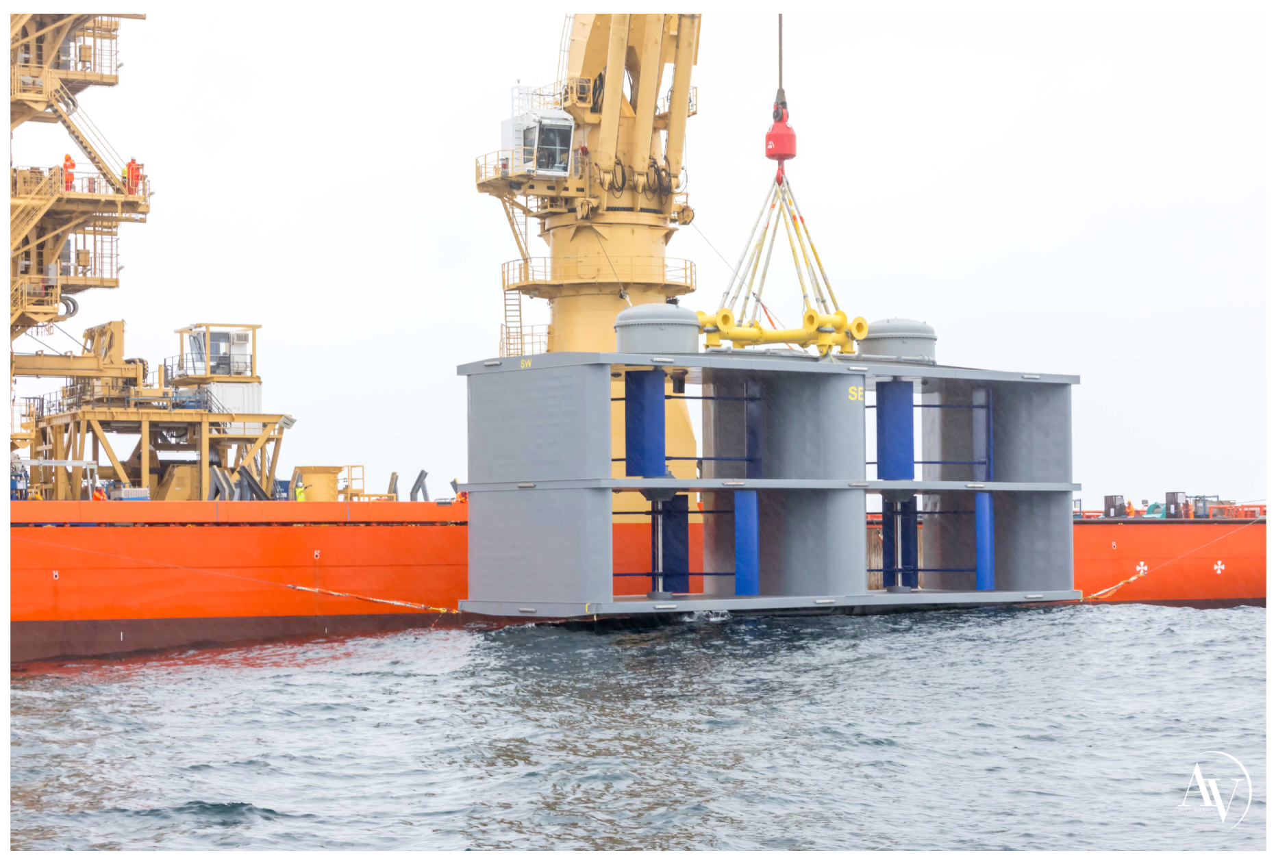To optimize cost and power, tidal turbines are likely to be installed on tidal farms [1]. At present, there is no industrial-scale tidal farm in operation; however, projects involving the deployment of turbines are being implemented. These projects are poised to establish the foundation for the development of industrial farms. This work is part of such a project, the OceanQuest project. OceanQuest’s technology is the HydroQuest turbine, a vertical-axis, bottom-mounted device, as shown in Figure 1.

Prior to undertaking a comprehensive examination of the numerous studies on tidal turbines, it is essential to provide a synopsis of the environmental context within which these turbines operate. Although highly localized, tidal sites can be found on almost every continent on Earth. Most of them are exposed to wind and waves [2,3]. These surface disturbances propagate through the water column and influence the flow. As shown in the analysis of in situ measurements in [4], sea states greatly affect load fluctuations without changing the average value. The bottom roughness also affects the stream and generates a high level of ambient turbulence of up to $20\%$ [5]. The ambient turbulence is site-specific and should be considered with great care when studying the implementation of a tidal site [2]. Turbulence characteristics and vortex size have also been shown to be affected by local roughness and may differ from one place to another within the same site [6,7,8]. Ambient turbulence influences the behavior of tidal turbines. Experimental and numerical studies have been performed on both vertical-axis tidal turbines (VATTs) and horizontal-axis tidal turbines (HATTs) to assess their effects [1,9,10,11]. From these investigations, turbulence was found to accelerate wake recovery, reduce the average power coefficient, and increase the load fluctuations. Investigations on tidal turbine arrays should therefore take this phenomenon into account.

In order to study tidal turbines and their environments, three possible approaches are available. The first and most cumbersome is in situ deployment, which has been successfully used to test prototypes and measure tidal flow characteristics [2]. This approach provides extremely valuable data but is expensive and very localized within tidal areas. Flume tank experiments are also used to test various tidal turbine technologies [11,12]. Access to the flow surrounding the turbines facilitates the acquisition of comprehensive and sophisticated statistics on flow and turbine behavior [13]. The main disadvantages of these approaches are the scale effects and the possible unrealistic blockage of the flow by the device. Experimental approaches are often used along with Computational Fluid Dynamics (CFD) approaches. It is acknowledged that numerical methods require experimentation for validation; nevertheless, these methods facilitate the creation of a full-scale model.

CFD VATT modeling techniques can be sorted into different categories based on increasing complexity and computational costs. The least expensive way to model turbines within a CFD simulation is the actuator cylinder approach coupled with the Reynolds-Averaged Navier–Stokes (RANS) solver [14]. This approach can be used to model large-scale arrays but can be inaccurate when complex and unsteady flows are considered. On the other side of the spectrum are blade-resolved simulations [15]. These approaches are the most accurate. Using state-of-the-art blade-resolved CFD, the authors of [15] were able to model two VATT models interacting. Even with access to large HPC centers, the computational cost of blade-resolved CFD is prohibitive when considering an array of more than two turbines. An interesting alternative is the Actuator Line Model (ALM) coupled with Large Eddy Simulation (LES) [16,17]. While less expensive than blade-resolved approaches, ALM–LES enables an unsteady description of the flow and tracking of the blades.

Due to its ability to capture unsteady phenomena, the ALM–LES method has been used to study advanced turbine behavior such as blade fatigue in HATT arrays [18]. When combined with a seabed morphology boundary condition, ALM–LES can model full-scale tidal turbines at actual tidal sites [19]. Regarding VATTs, [20,21] extensively examined the influence of ALM parameters on the accuracy of the model. Their findings are therefore extremely valuable for setting up a robust ALM–LES model. These investigations suggest that ALM–LES is an interesting tool for studying small arrays of full-scale vertical-axis tidal turbines.

Tidal turbine technology is not as well-established as wind turbine technology, and there are almost as many turbine technologies as there are manufacturers. Because these technologies behave differently, studies are required to optimize each design. The VATT in question here, the HydroQuest tidal turbine, has its own particularities and features four counter-rotating rotors distributed across two columns. The behavior of this specific turbine has been studied in model-scale experiments [11], in which unsteady upstream conditions were considered. A full-scale HydroQuest VATT was studied in [16] under various turbulent upstream conditions. To the best of the authors’ knowledge, no study has examined the interaction between multiple VATTs with counter-rotating rotors under realistic upstream conditions. The aforementioned setup includes complex interactions between unsteady phenomena and turbines. In light of the existing literature, ALM–LES appears to be a suitable methodology.

The ALM–LES method is implemented here within the Lattice Boltzmann Method (LBM) to calculate flow. The LBM is an efficient unsteady, weakly compressible CFD method that is well-suited for modeling large areas [8,22]. It also has low dissipation, making it well-suited for modeling the advection and dissipation of wakes. In the case of submerged water flow, simulations are well below the LBM compressibility limits. The LBM code is the PaLaBoS library [23]. ALM–LBM–LES is used in this paper to study full-scale HydroQuest turbines. Ambient turbulence is accounted for by generating a realistic turbulent boundary layer upstream of the turbines using a Synthetic Eddy Method (SEM) [24]. To avoid introducing too many unknown sources of disruption, the free surface and rough bottom are disregarded. Interactions between turbines are studied for six layouts with up to four turbines. The spacing and arrangement of the elements along the streamwise direction vary between cases. The analysis focuses on how the flow and power output are influenced by the relative distances and positions of the turbines. This paper is organized as follows. Section 2 introduces the numerical models, turbine specifications, and arrangements. Section 3 investigates the averaged flow and power, as well as the morphology of the wake. Section 4 presents the conclusions and perspectives.

Figure 1. HydroQuest/CMN tidal turbine tested at Paimpol-Bréhat (Brittany, France). Reproduced with permission from HydroQuest [25], 2022.

Figure 1. HydroQuest/CMN tidal turbine tested at Paimpol-Bréhat (Brittany, France). Reproduced with permission from HydroQuest [25], 2022.

2. Materials and Methods

2.1. Governing Equations

The LBM is a weakly compressible, unsteady CFD model derived from the Boltzmann equation [26]. Assuming that the fluid is isothermal and has a low Mach number, it is equivalent to a second-order finite-volume approach based on the Navier–Stokes equation. Unlike the latter, the LBM solves the problem at a mesoscopic scale. The behavior of groups of molecules is statistically represented with distribution functions. A distribution function is the density of molecules at a specific time and place that have a certain velocity. Interactions between molecules are modeled with the collision operator $\mathrm{\Omega }$, as shown in Equation (1). $f_i^{\prime }$ represents the post-collision distribution functions. The simulations presented in this paper are run with the open-source LBM library Palabos [23]. Palabos offers a wide range of collision operators depending on the physics at play. For studying tidal turbines with actuator lines, a regularized collision operator is selected [27,28].

$$f_i^{\prime }(\mathit{x},t)=\mathrm{\Omega }\left(f_i(\mathit{x},t)\right).$$

(1)

This collision operator does not add too much complexity to the scheme and provides enough stability and accuracy for the applications presented here. The stencil for velocity discretizations has 27 directions of propagation and is commonly referred to as $D3Q27$. Each node of the lattice now has 27 distribution functions ($f_i$), one per direction. The displacement of groups of molecules is performed during the streaming stage, preceded by the collision. Equation (2) shows the streaming equation:

$$f_i(\mathit{x}+c_i\Delta t,t+\Delta t)=f_i^{\prime }(\mathit{x},t)),$$

(2)

where $c_i$ represents the directions of the $D3Q27$ stencil and $\Delta t$ is the time step. The Large Eddy Simulation model is a constant Smagorinsky model. It is implemented in the LBM with the approach described in [29].

$${\mathit{S}}_{\alpha \beta }={\mathbf{\Pi }}_{\alpha \beta }^{neq}{\displaystyle \frac{1}{2}}{\displaystyle \frac{\rho \tau c_s^2-\sqrt{{\rho }^2{\tau }^2{c}_s^4+2C_s^2\parallel {\mathbf{\Pi }}_{\alpha \beta }^{neq}\parallel \rho }}{C_s^2\parallel {\mathbf{\Pi }}_{\alpha \beta }^{neq}\parallel \rho }}.$$

(3)

$${\mathbf{\Pi }}_{\alpha \beta }^{neq}=\sum _{i=0}^{27}\left(c_{i\alpha }{c}_{i\beta }{f}_i^{neq}\right)-{\delta }_{\alpha \beta }{c}_s^2.$$

(4)

The strain rate tensor ${\mathit{S}}_{\alpha \beta }$ is computed locally using Equation (3). The variable $\rho$ is the fluid density in lattice units, $\tau$ is the LBM relaxation rate, and the speed of sound in lattice units is $c_s=1/\sqrt{3}$. The tensor ${\mathbf{\Pi }}^{neq}$ is calculated using Equation (4), where $c_{i\alpha }$ is the ${\alpha }^{\mathrm{th}}$ component of the $i^{\mathrm{th}}$ direction of the $D3Q27$ stencil. The symbol ${\delta }_{\alpha \beta }$ is the Kronecker symbol, and $f_i^{neq}$ represents the non-equilibrium distribution functions. The Smagorinsky coefficient is $C_s=0.1$.

2.2. Actuator Line Model

Blade-resolved approaches require either a grid spacing inferior to $y^{+}=1$ in the boundary layer, or a sophisticated wall model. Even with the latter, it can be quite challenging to predict flow separation [30]. Both require large computational resources for high Reynolds-number simulations. In order to save computational resources and keep the benefit of the unsteadiness, an Actuator Line Model is used here. An ALM represents the blade action on the fluid through a forcing term in the LBM collision equation. An actuator line is placed where the blade should be. These lines comprise multiple point elements. The forcing term is calculated at the location of these elements. ALM input data are the tabulated lift coefficient $C_L$, the tabulated drag coefficient $C_D$, and the fluid velocity interpolated at each element $U_{rel}$. The algorithm by Shamsoddin and Porté-Agel (2016) [31] is implemented. It takes into account the dynamic stall of the blade during rotation. The force is calculated using Equation (5):

$${\displaystyle \frac{{\mathit{f}}_{AL}}{\rho }}=(c\Delta l)\left({\displaystyle \frac{U_{rel}^2}{2}}\right)(C_{L_{DS}}{\mathit{e}}_L+C_{D_{DS}}{\mathit{e}}_D),$$

(5)

where $C_{L_{DS}}$ and $C_{D_{DS}}$ are the coefficients modified by the dynamic stall algorithm. c is the chord, and $\Delta l$ is the spacing between two elements. The vectors ${\mathit{e}}_L$ and ${\mathit{e}}_D$ form the local frame of reference. In the dynamic stall algorithm, the derivative of the angle of attack with respect to the azimuth angle of the blade is obtained through a cubic spline interpolation of the average angle of attack. The angle of attack is averaged over 15 revolutions of the turbine. This implementation was validated by Grondeau et al., (2019) [16]. Time-averaging the angle of attack can eliminate variations in incidence caused by turbulence. However, since this study does not focus on load fluctuations, the influence of time-averaging on the averaged power coefficient and wake should be minimal. The model still takes into account instantaneous variations in velocity $U_{rel}$. The ALM–LBM–LES approach was successfully used to model a VATT placed inside a turbulent boundary layer. Three meshes were used to evaluate the influence of grid spacing. The numerical results were found to be in good agreement with the experimental data, especially for the shape of the wake and the velocity deficit, as shown in Figure 2.

To remain consistent with [16], the same parameters are selected. The spacing between two ALM elements along a line is equal to the grid size, $\Delta x=0.257$ m. To avoid discontinuities and instabilities, the ALM force is distributed around each ALM element using Equation (6), where $\eta (ϵ,d)$ is the distribution kernel.

$${\mathit{f}}_{AL}\left(\mathit{x}\right)=\eta (ϵ,d){\mathit{f}}_{AL}.$$

(6)

$$\eta (ϵ,d)={\displaystyle \frac{1}{{ϵ}^3{\pi }^{3/2}}}exp\left(-{\left({\displaystyle \frac{d}{ϵ}}\right)}^2\right).$$

(7)

The distribution kernel is described in Equation (7). The variable d is the distance between an ALM element and a node of the lattice where the force is distributed. The kernel parameter $ϵ$ is equal to $2\Delta x=0.514$ m [21]. The fluid velocity $U_{rel}$ is interpolated using the distribution kernel. The mesh is described in Section 2.4.

2.3. Turbine Specifications

The present study examines a vertical-axis tidal turbine designed and manufactured by HydroQuest (Grenoble, France) 1 and CMN (Construction Mécanique de Normandie, Cherbourg, France). The turbine is equipped with four rotors, each consisting of three blades, as illustrated in Figure 1. The rotors have straight blades and are of the Darrieus H-type. The left-hand side and right-hand side rotors are counter-rotating. The blade profile is based on the NACA0018 profile. The specific details regarding the blade’s profile and chord remain proprietary and are not disclosed. The lift and drag coefficients are calculated with the XFLR5 software v6.61 2, using the following parameters: $Ma=0$, $N_{crit}=9$, and 300 panels. Depending on its azimuthal angle, the turbulence intensity, or its location within the boundary layer profile, the blade experiences varying Reynolds numbers. Consequently, calculations with XFLR5 are executed within the range of Reynolds numbers from $7\times {10}^4$ to $6\times {10}^6$. The rotor characteristics are summarized in

Table 1. Configuration of the rotor.

Quantity	Value	Unit
Tip-speed ratio $\lambda$	$1.5$	~
Reynolds number based on radius	$5.9\times {10}^6$	~
Radius R	$4.0$	m
Height of the blades H	$3.8$	m

.

The rotor’s axis, connectors, and blades are modeled using actuator lines. Only the blade ALM model uses the tabulated $C_L$ and $C_D$. The axis and the H-connectors have constant drag. The axis has a drag coefficient of $C_{D_{axis}}=1$, and the drag of the H-connectors is evaluated with Ansys Fluent (v14.5, Ansys Inc., Canonsburg, PA, USA). The stator boundary condition is enforced at its surface location using the boundary condition from [33]. A free-slip condition is applied. Figure 3 depicts the turbine model. The gravity base is not modeled. The distance between the bottom of the stator and the seabed is 5 m. An equivalent diameter, representative of the turbine width, is defined for the turbine and is $D_{eq}=25.0$ m.

2.4. Turbine Layout and Simulation Setup

In total, 6 turbine layouts are investigated: 3 aligned scenarios and 3 staggered scenarios. The streamwise distance between turbines varies for each scenario. The distance between the turbines is defined from the rear of the upstream turbine stator to the front of the downstream turbine stator. The investigated distances are $50.0$ m, $100.0$ m, and $150.0$ m. The aligned layouts have 3 turbines, and the staggered layouts have 4 turbines. The depth of the domains is constant across all scenarios and is set to a realistic value of $43.12$ m, considering a tidal site like the Alderney Race. The domains also have a constant width of approximately $20D_{eq}=500$ m. The length of the numerical domains depends on the distance between the turbines. The dimensions of the domains are summarized in

Table 2. Turbine layouts.

Scenario	Layout	x-Spacing	y-Spacing	x-Length
$3T_1$	3 aligned	50 m	~	560 m
$3T_2$	3 aligned	100 m	~	660 m
$3T_3$	3 aligned	150 m	~	760 m
$4T_1$	4 staggered	50 m	70 m	560 m
$4T_2$	4 staggered	100 m	70 m	660 m
$4T_3$	4 staggered	150 m	70 m	760 m

, along with identifiers for each layout. For the $3T_i$ scenarios, the most upstream turbine is designated as the first one, the one in between as the second, and the most downstream one as the third. For the $4T_i$ scenarios, the most upstream turbine is designated as the first, the turbines in the second row are the second and third, and the most downstream one is the fourth.

As in most LBM simulations, the domain is discretized using Cartesian grids. Each mesh is composed of three grids, with a $\Delta x$ and $\Delta t$ ratio of two between neighboring grids. The grid with the smallest spacing contains the turbine and the close wake. The grid with the intermediate spacing is used to calculate the domain between the turbines and the wake further away from the turbines. The rest of the domain is solved on the coarsest grid. The mesh is illustrated in Figure 4 and Figure 5. The finest grid has a spacing of $\Delta x=0.257$ m, which is chosen following the convergence study carried out by Grondeau et al., (2019) [16]. The time step in the finest grid is $\Delta t=5.27\times {10}^{-3}$ s. In the LBM, the time step $\Delta t$ is imposed through the physical speed of sound of the fluid. This usually yields an extremely small time step. When acoustic effects are not considered, it is common practice to artificially decrease the speed of sound in the fluid. In this case, the hydrodynamic results are valid up to a Mach number of $0.3$. For the current study, the Mach number computed with the velocity $U_{x_{\delta }}$ is $Ma=0.05$, well below the limit of $0.3$ required by the LBM. The total number of nodes for each scenario is given in

Table 3. Computational effort for the ALM–LBM–LES simulations. Time spent refers to the wall-clock time.

Scenario	Nodes	N Processors	Time Spent/Revolution
$3T_1$	$29\times {10}^6$	280	1654 s
$3T_2$	$35\times {10}^6$	280	1972 s
$3T_3$	$39\times {10}^6$	280	2133 s
$4T_1$	$42\times {10}^6$	420	1702 s
$4T_2$	$46\times {10}^6$	420	1837 s
$4T_3$	$50\times {10}^6$	420	1810 s

.

The inlet of the numerical domain is a Dirichlet velocity boundary condition. A SEM boundary condition is added to it in order to generate realistic turbulence [34]. The average axial velocity profile is constant in the y-direction and is set to match measurements made in the Alderney Race [35]. It is illustrated in Figure 6 and is calculated as

$$U_x\left(z\right)=U_{x_{\delta }}{\left({\displaystyle \frac{z}{\delta }}\right)}^{{\displaystyle \frac{1}{n}}},$$

(8)

where z is the distance from the seabed and $U_{x_{\delta }}$ is the average velocity at $z=\delta$. In this study, $\delta =10.0$ m, $U_{x_{\delta }}=1.475$ m.s ⁻¹, and $n=6.5$. The flow velocity in the Alderney Race varies significantly depending on the location. The value we chose was not measured at the maximum velocity location and is consistent with the first deployment site at Paimpol-Bréhat. The SEM is calibrated to generate turbulence with an intensity that could be encountered in a real-life tidal site. Figure 7 plots the turbulence intensity measured within the ALM–LBM–LES simulation, 50 m upstream of the most upstream turbine. The sizes of the SEM vortices were set to a constant value of 8 m. In Grondeau et al., (2022) [9], the integral length scale of the turbulence was quantitatively linked to the prescribed size of the SEM vortices. Using a vortex size of 8 m should then produce an integral length scale of approximately 8 m. This value was chosen to match the average integral length scale ${\mathcal{L}}_z$ measured in the Alderney Race [36]. Velocity Dirichlet boundary conditions are applied to the top and side planes of the domain according to the velocity profile depicted in Figure 6. Spalding’s boundary layer velocity profile [37] is applied to the boundary located at the bottom of the domain. A constant pressure is imposed at the outlet of the numerical domain.

3. Results and Discussion

In this section, the results from the simulations of the aligned scenarios ($3T_i$) and the staggered scenarios ($4T_i$) are presented and discussed. The simulations were run for 530 s before calculating the statistics. This duration is approximately one channel flow-through time for the $3T_3$ and $4T_3$ scenarios. The statistics were sampled over 244 s, with a frequency of 190 Hz. According to [38], a minimum of 20 turbine revolutions is required to average the data. With a TSR of $1.5$, it took the turbine approximately 11 s to complete a single revolution. In 244 s, the turbine completed 21 revolutions, which is more than what is recommended by [38]. For all layouts, the focus is primarily on the wake velocity, then on the power output, and finally on the wake morphology.

3.1. Computational Effort

Table 3 summarizes the computational effort required for the six ALM–LBM–LES simulations. All computations were carried out on the CRIANN (Centre Régional d’Informatique et d’Applications du Numériques de Normandie) cluster Myria 3.

3.2. Wake Velocity

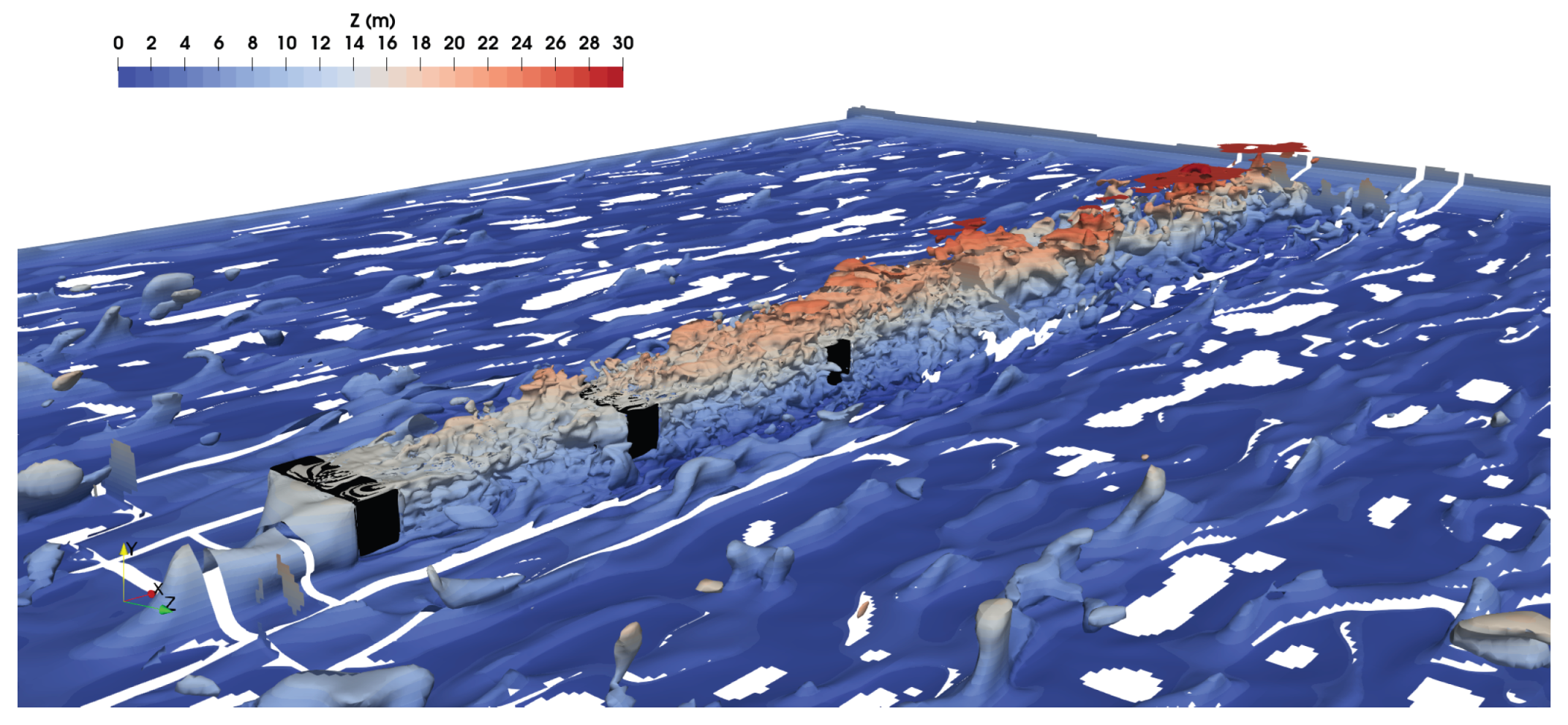
An instantaneous 3D view of the streamwise velocity for the $3T_3$ scenario is shown in Figure 8. Since this scenario has the largest spacing between turbines, it is interesting to note that downstream turbines are located in areas affected by the wake. Moreover, it was qualitatively observed that the ambient vortices had a size on the same order of magnitude as the turbines, reflecting the prescribed SEM vortex length of 8 m. Because of the computational cost of this study, the simulations were not run long enough to compute advanced statistics, such as autocorrelation, which could have provided a quantitative estimation of the actual size of the vortices.

Investigating how turbine spacing affects the wake can be tedious, as the wake is a 3D, unsteady phenomenon that occupies a large volume. To obtain a global view of the wake with a manageable amount of data, a limited set of quantities was selected. The averaged axial velocity deficit was plotted along the turbine centerline for all scenarios. The velocity deficit is defined as $U_{Def}=(U_{x_{\delta }}-U_x)/U_{x_{\delta }}$. Figure 9 shows the velocity deficits for the $3T_i$ scenarios. In all scenarios, wake recovery is not achieved between turbines, and downstream turbines are always located in regions with reduced velocity. Also, the velocity deficit upstream of the third turbine is greater than that upstream of the second turbine. This was observed across all three scenarios. The velocity deficit accumulates with each successive turbine, as also observed by [14]. After approximately 1 $D_{eq}$, the velocity recovery follows a linear trend, with a similar trend observed across all cases and turbines. This behavior is examined in more detail later in this section. The peak velocity deficit at each turbine varies depending on the turbine and the scenario, and no consistent trend was observed (see Figure 9). As the statistical line passes through the interior of the stator, the quantities calculated at the turbine location have little physical meaning.

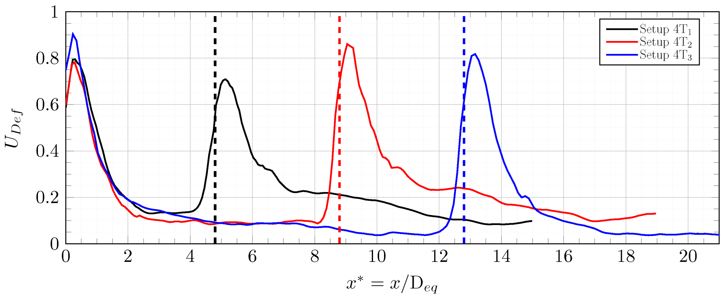
In the $4T_i$ scenarios, the turbines are not aligned, so two figures are needed to show the velocity deficit along the x-direction. Figure 10 shows $U_{Def}$ for central turbines 1 and 4. The velocity deficit upstream of turbine 4s varies significantly across scenarios. For the $4T_3$ scenario, the wake of turbine 1 almost fully recovered, so its influence on turbine 4 should be minimal. As in the $3T_i$ scenarios, a linear trend was observed in the far wake of each turbine. 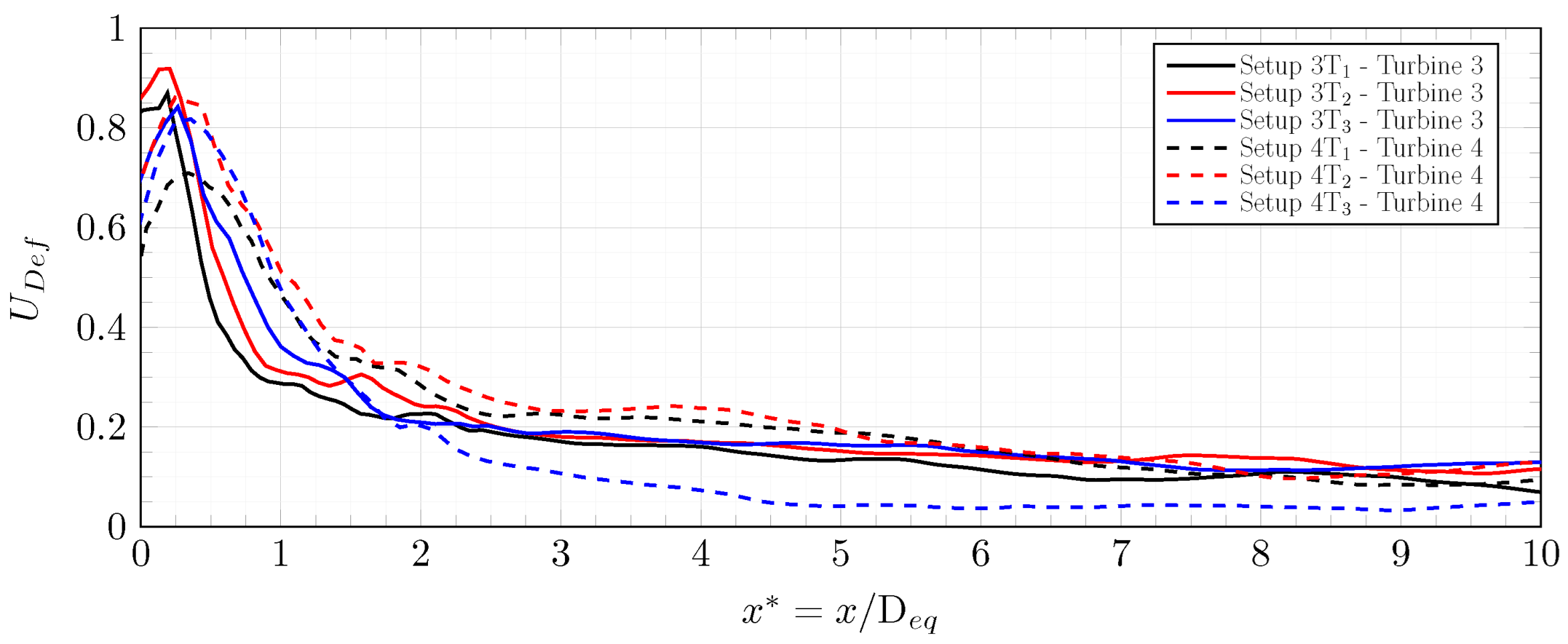Figure 11 shows $U_{Def}$ for lateral turbines 2 and 3, and no clear differences between the scenarios are visible. More differences may appear in integral quantities, such as the power coefficient, or in the 3D plots of the wakes examined in the following sections.

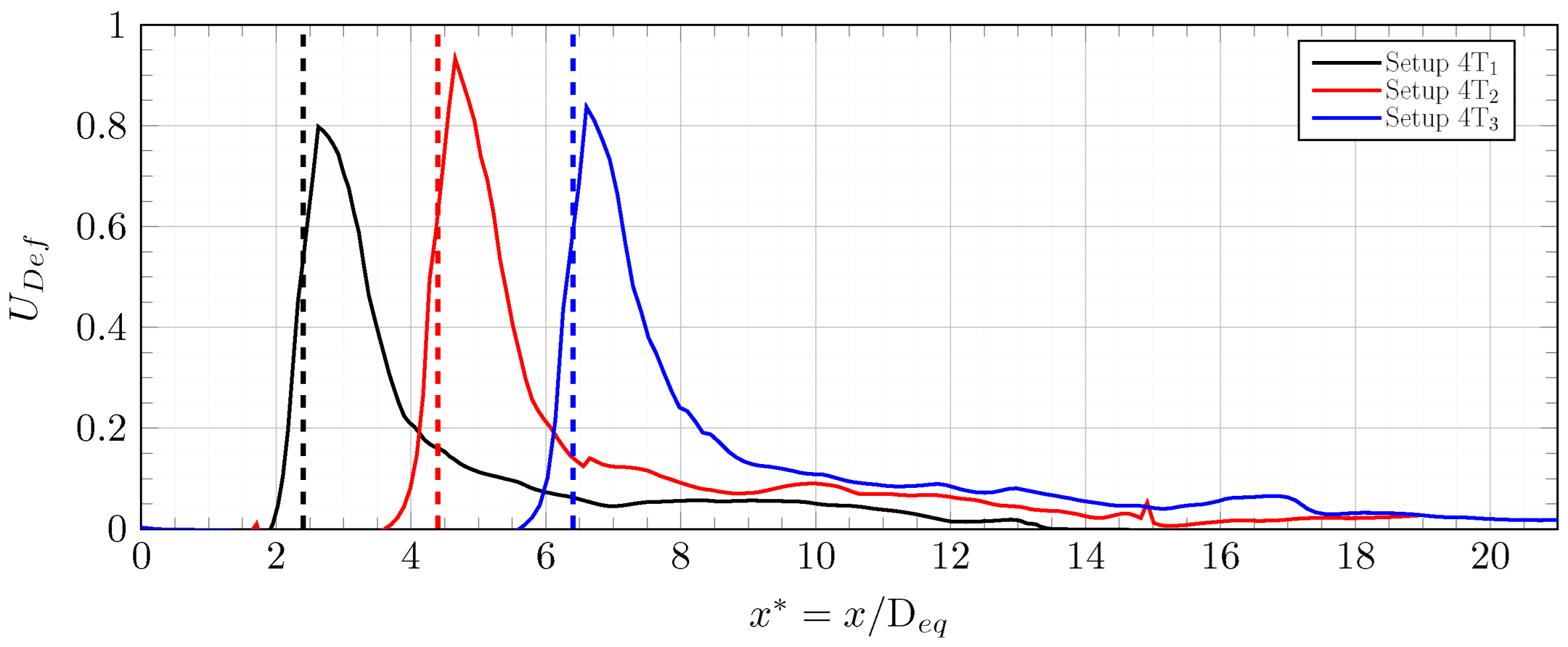
For better comparison between arrays, two additional figures are included. Figure 12 shows the wake downstream of the last turbine in the $3T_i$ and $4T_i$ scenarios. As noted previously, all velocity deficit plots exhibit a linear trend after approximately 1 $D_{eq}$. All scenarios are highly similar, with one exception: the velocity deficit downstream of turbine 4 in the $4T_3$ scenario is significantly lower than in the other scenarios. This is consistent with the results in Figure 10. 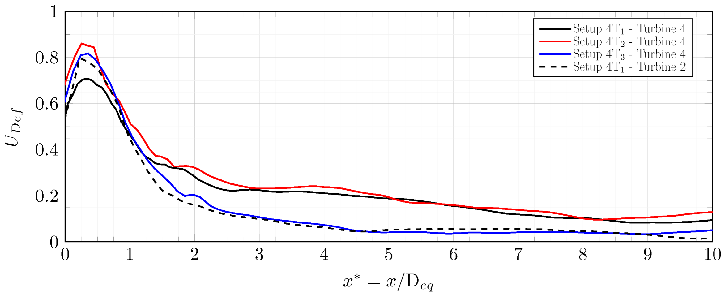Figure 13 compares the wake of turbine 4s in the $4T_i$ scenarios with the wake of turbine 2 in the $4T_1$ scenario. Indeed, turbine 2 in the $4T_1$ scenario is isolated and almost undisturbed. As seen in Figure 13, the wake of turbine 4 in the $4T_3$ scenario is almost identical to that of an undisturbed turbine.

The results in Figure 9, Figure 10, Figure 11, Figure 12 and Figure 13 suggest that the spacing between turbines and the number of turbines in the array do not significantly affect the velocity deficit downstream of the array. This remains true up to a critical spacing, beyond which the wake of an upstream turbine can fully recover. In such a scenario, the velocity deficit downstream of the array is similar to that of an isolated turbine. This critical spacing lies between 200 m and 300 m. As shown in Figure 10, the corresponding critical velocity deficit upstream of the turbine falls within the range $\left[0.05,0.1\right]$.

3.3. Turbine Power

In this section, the average power coefficients of the turbines in the $3T_i$ and $4T_i$ scenarios are investigated. The power coefficients are made dimensionless by dividing the power coefficient of each turbine by that of the first turbine of the corresponding layout, $3T_3$ or $4T_3$, as shown in Equation (9).

$$C_P^{*}(T_i,3T_i)={\displaystyle \frac{C_P(T_i,3T_i)}{C_P(T_1,3T_3)}},C_P^{*}(T_i,4T_i)={\displaystyle \frac{C_P(T_i,4T_i)}{C_P(T_1,4T_3)}}$$

(9)

A distinction is made between top rotors and bottom rotors. In the figures below, the power coefficients of the bottom rotors are shown in dull colors, while those of the top rotors are shown in bright colors. The power coefficients for the $3T_i$ scenarios are shown in Figure 14. Across all scenarios, turbine 1s have the highest $C_P^{*}$ values and turbine 3s have the lowest. The loss in $C_P^{*}$ for turbine 3s is substantial. All turbine 3s have $C_P^{*}$ values approximately $60\%$ lower than those of turbine 1s. This is consistent with the results in Section 3.2, where an accumulation of the velocity deficit for downstream turbines was observed. 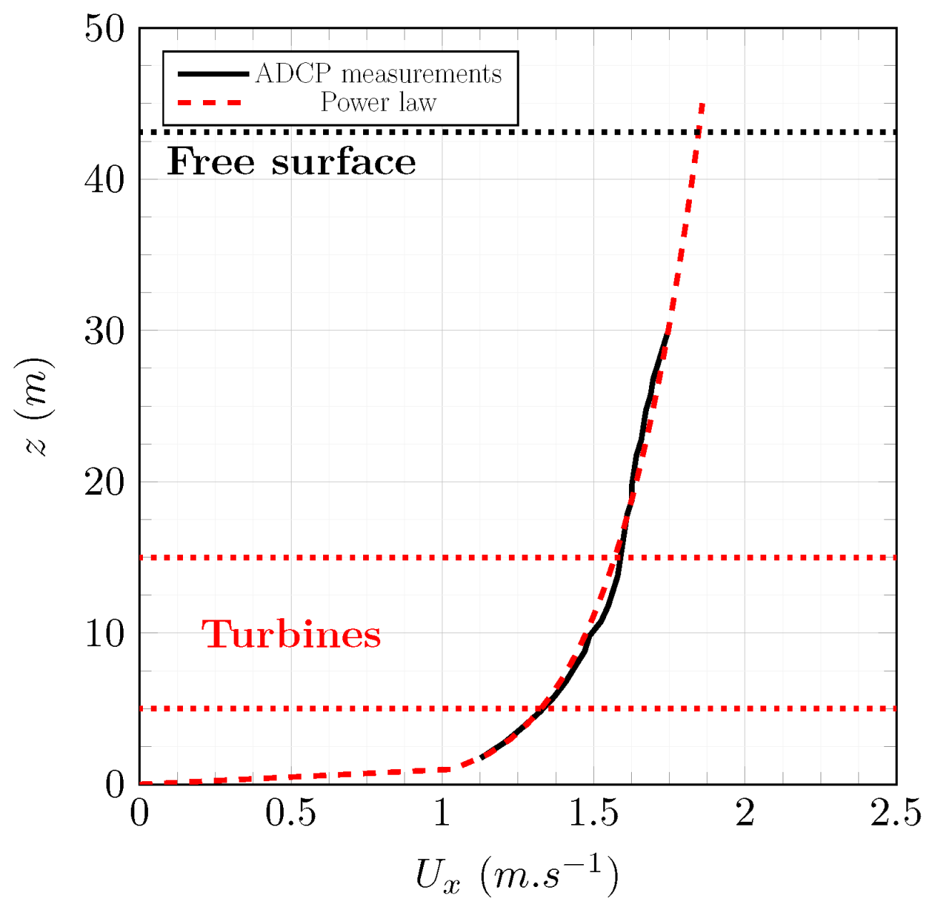The top rotors of turbines 1 and 2 have higher $C_P^{*}$ values than the bottom rotors. This is likely due to the upstream boundary layer shown in Figure 6. The difference in $C_P^{*}$ between the top and bottom rotors is more pronounced for turbine 2s than for turbine 1s. No difference is observed for turbine 3s. Further insight into these two observations is given in Section 3.4, based on the velocity deficit maps. Turbine 1 in the $3T_1$ scenario generates slightly less power than turbine 1 in the $3T_2$ scenario, which generates less power than turbine 1 in the $3T_3$ scenario. This difference could be due to how the array affects flow blockage, but it is also small enough to fall within the method’s margin of error.

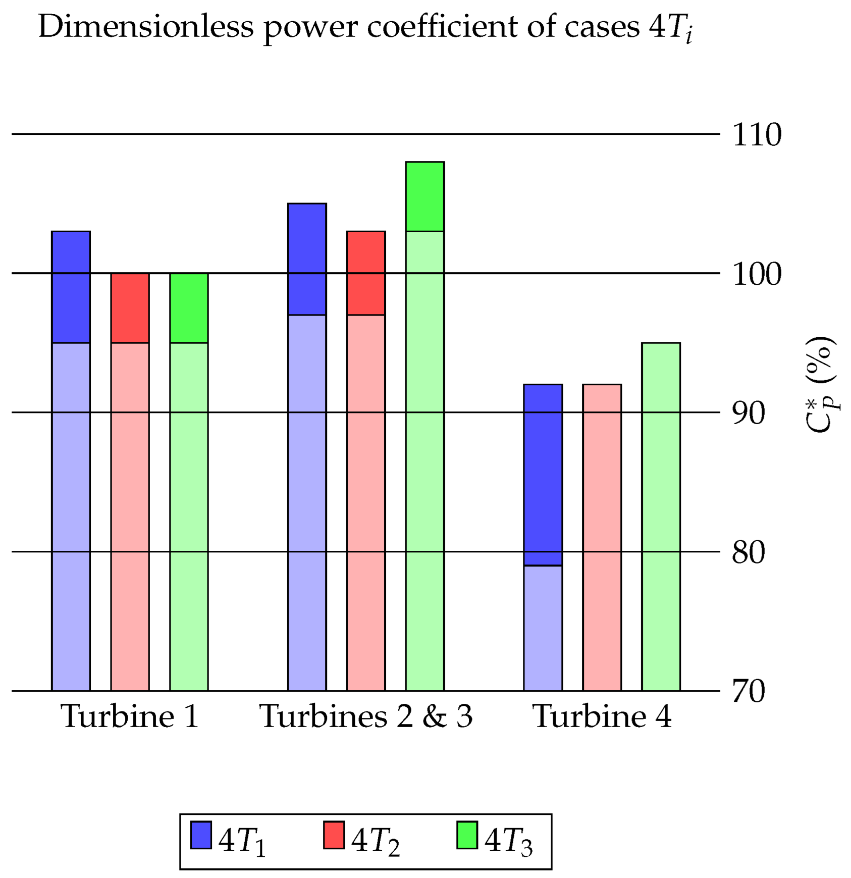
Figure 15 depicts the $C_P^{*}$ values for the turbines in the $4T_i$ scenarios. The power coefficients of all turbines fall within a narrower range compared to the $3T_i$ scenarios. The lowest power is observed in the bottom rotor of turbine 4 in the $4T_1$ scenario and is around $80\%$. Turbines 2 and 3 have higher $C_P^{*}$ values than turbine 1 and seem to benefit from the staggered configuration. The flow likely accelerates when bypassing the first turbines in the arrays, a known phenomenon in wind and tidal farms [14]. The gain in power is highest in the $4T_3$ scenario, with an $8\%$ increase in $C_P^{*}$. No difference between the top and bottom rotors is observed for turbine 4s, except in the $4T_1$ scenario. This is likely due to interactions between turbines and the expansion of the wake. Section 3.4 provides a more detailed analysis of this phenomenon.

Lin et al., (2024) [15] modeled two aligned VATTs using blade-resolved LES. By testing various distances between turbines, they observed that the power coefficient of the second turbine was halved when the distance between turbines was 10 diameters. In our case, the greatest reduction in power occurred in the $3T_1$ scenario, where the power coefficient of the second turbine decreased by 40%. In this scenario, the distance between turbines was 50 m, equivalent to two $D_{eq}$ or $6.25$ D. In addition to technological differences, Ref. [15] used a constant velocity inlet with no turbulence, which was not the case here. Turbulence is known to reduce the wake recovery distance. For example, in [1], the influence of the distance between two aligned HATTs was examined. Two inflow conditions were tested: one with a turbulence intensity of 3% and the other with 15%. With a distance of 12 D between turbines and a turbulence intensity of 3%, the power coefficient of the second turbine was reduced by 50%. However, with a distance of 6 D and a turbulence intensity of 15%, the reduction was only 20%. This could explain why, despite the shorter spacing compared to [15], the power coefficient reduction in our study was smaller.

It is worth noting that turbine 4s in the $4T_i$ scenarios and turbine 2s in the $3T_i$ scenarios have similar power coefficients. All are located in the wake of a single turbine. These observations are consistent with the velocity deficit upstream of these turbines, which lies between 10 and $20\%$.

3.4. Wake Morphology

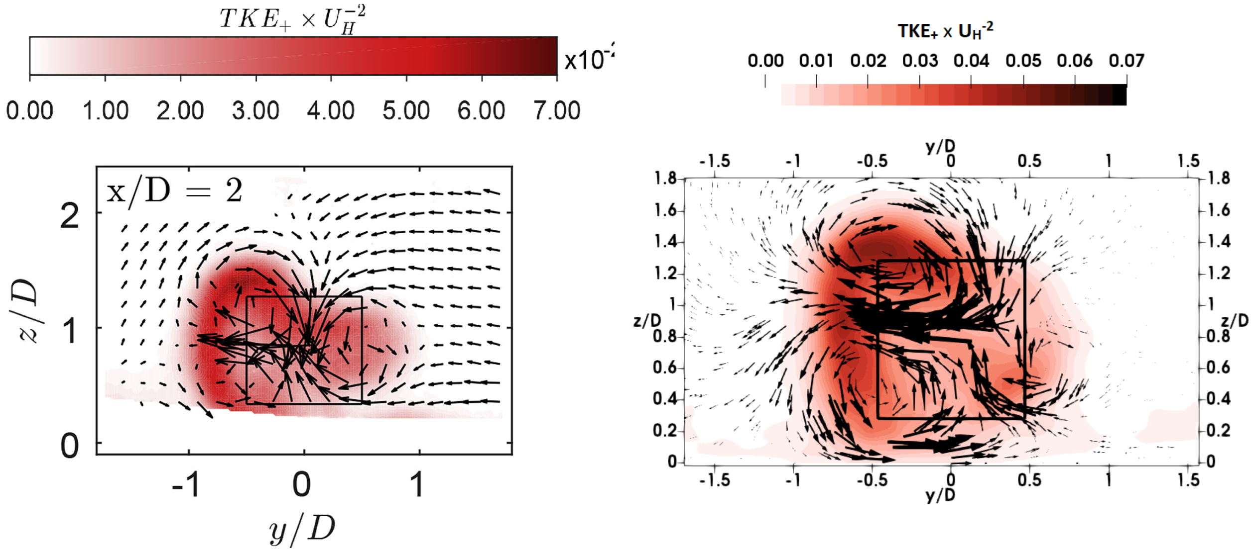
Grondeau et al., (2019) [16] studied the wake of a single HydroQuest turbine, identical to the one modeled here. To observe the shape of the wake, the average flow field was sliced with planes normal to $\overrightarrow{x}$ at several downstream distances. Two counter-rotating vortices were observed in the wake of the same turbine using this approach. A similar procedure was used in the $3T_i$ and $4T_i$ scenarios.

3.4.1. Wake Morphology for the Aligned Setup

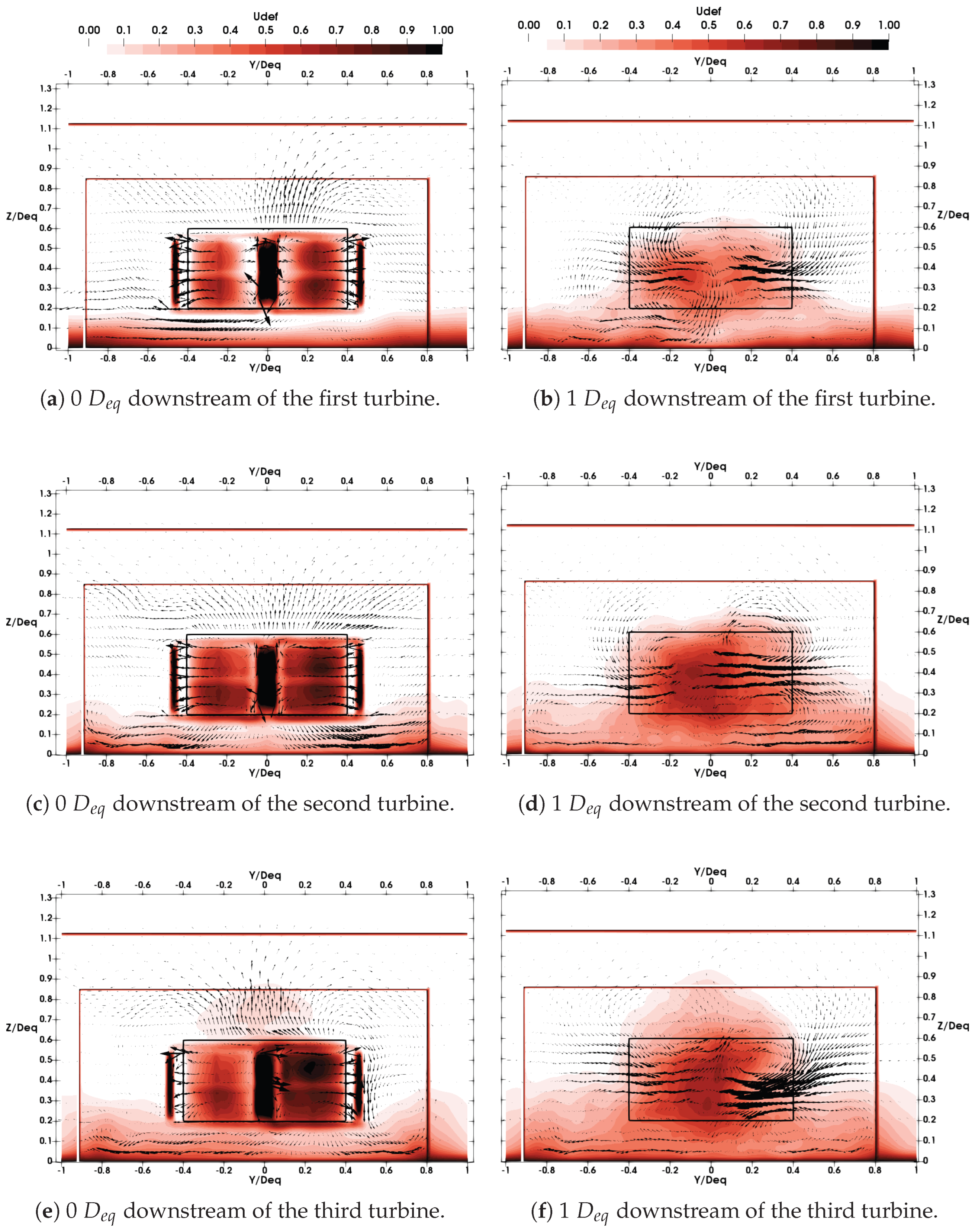
Starting with the most compact scenario ($3T_1$), the velocity deficit was plotted at two downstream distances for each turbine: $0D_{eq}$ (turbine location) and $1D_{eq}$. Recall that the spacing between turbines in this case is 50 m, or 2 $D_{eq}$. Figure 16a,b show the results for the first turbine; Figure 16c,d show the results for the second turbine; and Figure 16e,f show the results for the third and most downstream turbine. Looking at Figure 16a,c,e, the influence of upstream turbines on the second and third turbines is apparent. The boundary layer is thicker at the locations of turbines 2 and 3. Figure 16b,d,f depict the velocity deficit in the wakes of the turbines. The influence of upstream turbines on downstream turbines is even more noticeable. Counter-rotating vortices are observed, as reported in [16]. Top vortices have their centers located at the top of the turbine footprint, at about a quarter of the turbine width from the center. The intensity of the top vortices increases for the second and third turbines, modifying the shape of the wake. This stretches the bottom vortices toward the sides, although it has limited influence on the overall wake width, which is relatively similar between the second and third turbines. The most significant effect is the upward stretching of the wake toward the free surface.

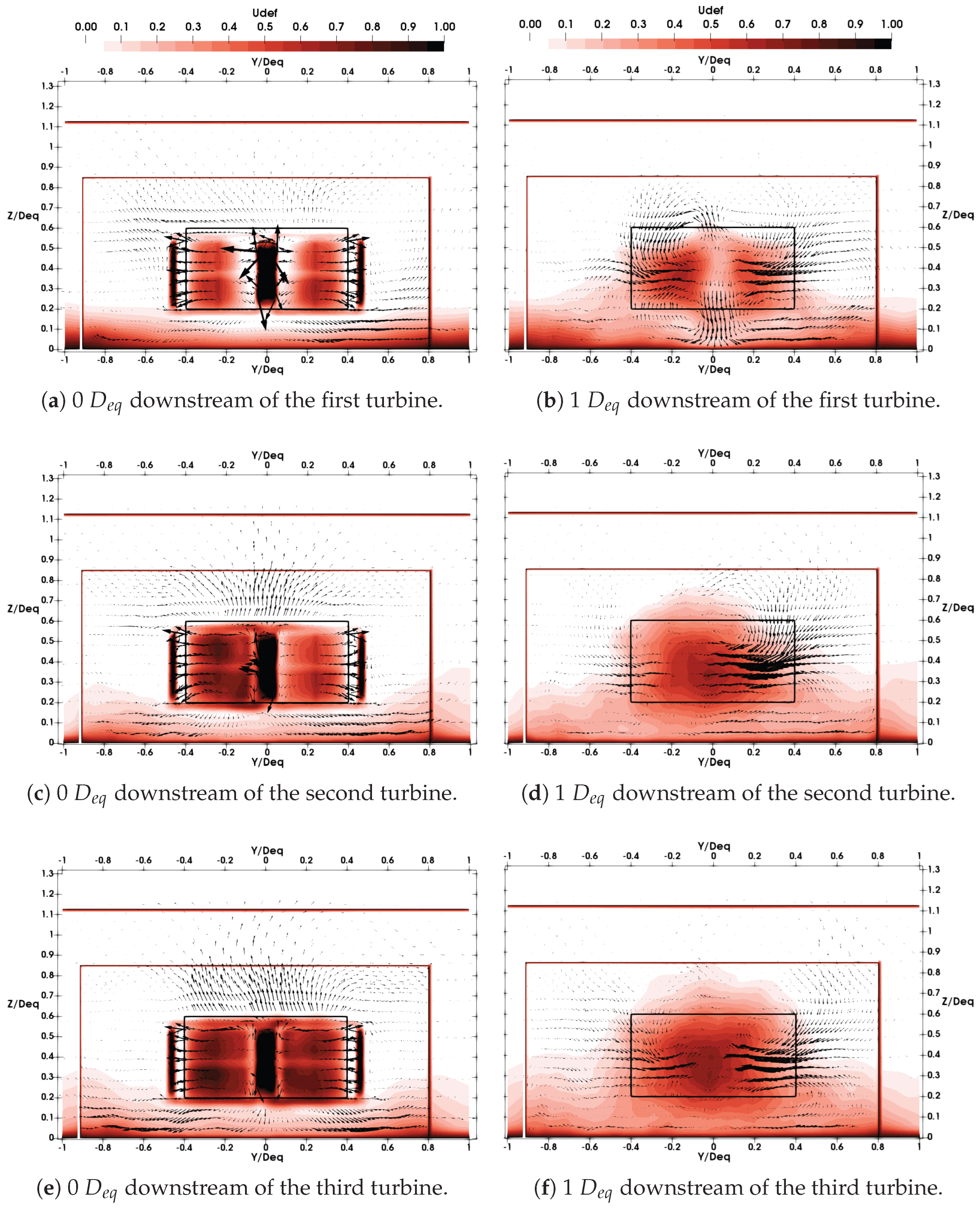
The second aligned scenario ($3T_2$), with a spacing between turbines of 100 m, is shown in Figure 17a–f. Differences can still be observed at the turbine locations, and the boundary layer is thicker for downstream turbines. The shapes of the wakes of turbines 1 and 2, as shown in Figure 17b,d, are similar. The main differences are that the wake footprint is larger and the velocity deficit is more pronounced for turbine 2. Only the wake of turbine 3 is stretched significantly upward.

The averaged velocity field for the $3T_3$ scenario, with a spacing between turbines of 150 m, is shown in Figure 18a–f. There is little difference between the boundary layers at the turbine locations. Additionally, the velocity fields shown in Figure 18c,e are almost identical. The wakes of turbines 2 and 3 are no longer mushroom-shaped but instead more rectangular, like that of turbine 1. Between turbines 2 and 3, the wake footprint spreads in the y- and z-directions, and the velocity deficit increases. The intensity of the counter-rotating vortices does not seem to increase between turbines.

The distance between turbines significantly affects the morphology of the wake. For spacings below 150 m, the counter-rotating vortices become more intense with each successive turbine. This greatly affects the shape of the wake by stretching it toward the surface, which can be seen in Figure 19. A 3D wake animation for the $3T_1$ scenario, based on the isocontour of the Lambda-2 criterion, is provided in the Supplementary Materials. Because only three turbines were modeled here, the effect on the array was limited. These vortices have also been described in experimental studies [32,39,40]. As explained in [32], the counter-rotating vortex pairs originate from the $U_z$ velocity gradient in the z-direction (see the original work for more details). Thus, an increase in this gradient for downstream turbines may cause the intensification of the vortices. Across all $3T_i$ scenarios, the wake footprint of the first turbine does not seem to extend beyond the turbine footprint. This is not the case for the wakes of turbines 2 and 3, consequently, turbine 3s are fully embedded in the velocity deficit region, whereas turbine 2s are not. Turbine 1s are only influenced by the upstream boundary layer. So, it is likely that the bottom and top rotors of turbine 3s experience a more uniform vertical velocity profile than those of turbines 1 and 2 due to the mixing caused by the wake. This may explain why the difference in $C_P$ between the top and bottom rotors, as discussed in Section 3.3, vanishes between turbines 2 and 3.

3.4.2. Wake Morphology for the Staggered Setup

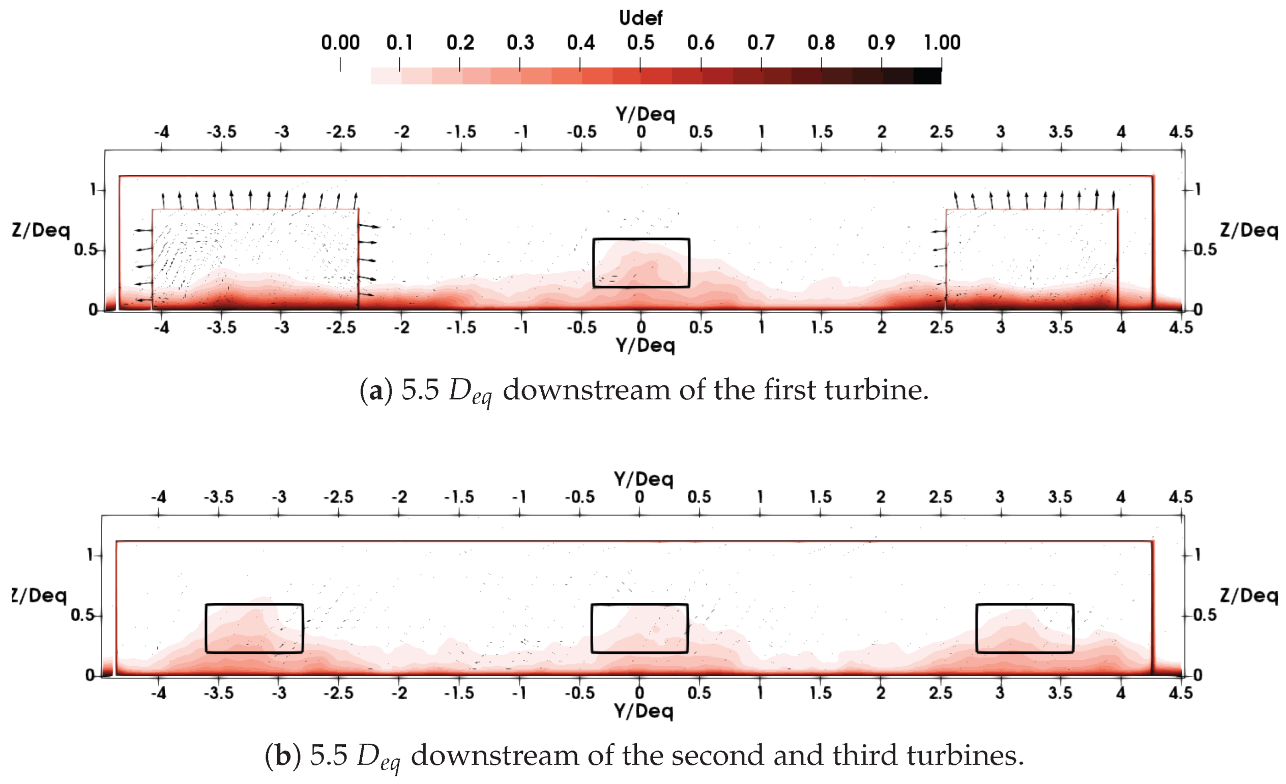
The procedure described at the beginning of Section 3.4 was applied to the $4T_i$ scenarios. For the $4T_1$ scenario, the average velocity deficit is shown in Figure 20 at $1.5D_{eq}$ downstream of the first turbine and $1.5D_{eq}$ downstream of the second and third turbines. This corresponds to $0.5D_{eq}$ upstream of the second, third and fourth turbines. In Figure 20a, the wake of the first turbine does not expand vertically beyond the turbine footprint. The wake is slightly wider than the turbine footprint but does not exceed $2D_{eq}$ in the y-direction. The counter-rotating vortices can be seen. As shown in Figure 20b, the wake of the first turbine creates a strong velocity deficit gradient in the z-direction. The velocity deficit is different between the top and the bottom of the turbine footprint and is estimated to be approximately $30\%$.

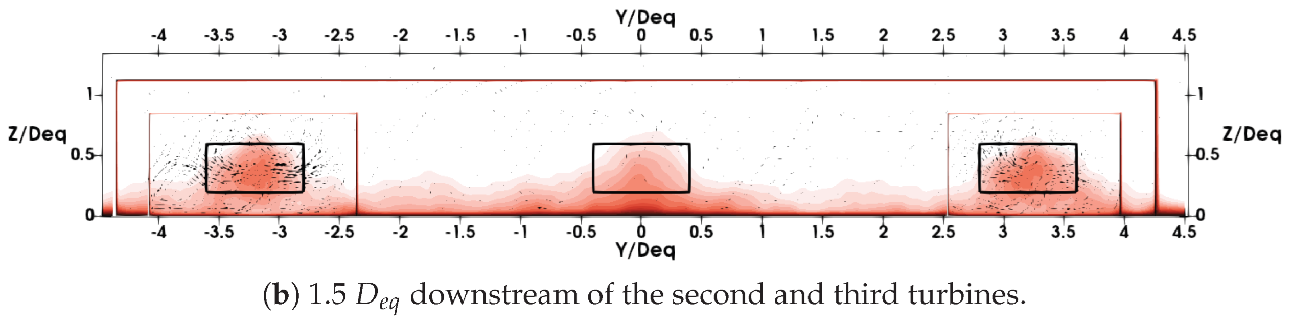
Figure 21a shows the velocity deficit $0.5D_{eq}$ upstream of turbines 2 and 3, or $3.5D_{eq}$ downstream of turbine 1. The wake expansion in the vertical direction is still restricted to the turbine footprint. In the y-direction, the wake expands up to $2D_{eq}$. No counter-rotating vortex is visible. Figure 21b shows the velocity deficit $0.5D_{eq}$ upstream of turbine 4, or $3.5D_{eq}$ downstream of turbines 2 and 3. The wakes of turbines 1, 2, and 3 are distinct from one another. The wake of turbine 1 covers all of turbine 4’s projected area. The difference in the velocity deficit between the top and bottom of turbine 4 is below $10\%$.

Figure 22a,b show the average axial velocity deficit $0.5D_{eq}$ upstream of turbines 2 and 3 and $0.5D_{eq}$ upstream of turbine 4, respectively. This corresponds to $5.5D_{eq}$ downstream of turbine 1 and turbines 2 and 3, respectively. The wake of turbine 1 expands beyond $2D_{eq}$ in the y-direction. As shown in Figure 22b, the wakes of turbines 1, 2, and 3 are still $1D_{eq}$ apart. The wake of turbine 1 is visible and covers most of turbine 4’s area, and the velocity deficit is almost uniform.

In Section 3.3, it was noted that in the $4T_2$ and $4T_3$ scenarios, the power coefficients of the top and bottom rotors of turbine 4s were identical. In the $4T_1$ scenario, a difference of $10\%$ was identified. This variation is likely attributable to disparate vertical velocity gradients present at the turbine locations. This gradient was relatively low for turbine 4s in the $4T_2$ and $4T_3$ scenarios, while it was higher in the $4T_1$ scenario. It was also noted in Section 3.3 that turbines within the second row benefited from the blockage produced by turbine 1. This resulted in higher $C_P$ values. As shown in the velocity deficit maps, the wakes of turbine 1s keep expanding in the y-direction. This would explain why the increase in $C_P$ was greater in the $4T_3$ scenario. This was not the case in the $4T_1$ and $4T_2$ scenarios, where the $C_P$ values of turbines 2 and 3 were close but the wake expansion differed. The vertical expansion of all the wakes of the $4T_i$ turbines was limited to the turbine footprints. This outcome was significantly different from that of the $3T_i$ scenarios, where the vertical expansion was amplified for multiple aligned turbines situated at distances less than 150 m from each other.

4. Conclusions and Outlook

ALM–LBM–LES simulations of realistic full-scale VATTs arranged into small arrays were performed. A total of six layouts were investigated: three aligned configurations with three turbines ($3T_i$ scenarios) and three staggered configurations with four turbines ($4T_i$ scenarios). The distances between consecutive aligned turbines were 50, 100, 150 m in the $3T_i$ scenarios, and 100, 200, 300 m in the $4T_i$ scenarios. All simulations used the same turbulent upstream boundary condition, generating a realistic inflow. The average velocity deficit along the turbine centerline was analyzed, as well as the average power coefficient and the shape of the wake.

It was observed that the centerline velocity deficit downstream of the array was not influenced by the number of turbines and that arrays $3T_i$, $4T_1$, and $4T_2$ exhibited similar wakes. The distance between turbines appeared to have a greater influence. Indeed, the wake in the $4T_3$ scenario differed significantly from the others. It was suggested that, in this scenario, there was a critical spacing of between 200 m and 300 m that led to a quasi-full recovery of the flow. This resulted in the far wake of the array being identical to that of a single turbine. The influence of different turbulence intensities on the far wake of a single HydroQuest VATT was assessed in [16] using the same numerical approach. The impact on both the velocity deficit and the shape of the wake was observed. Consequently, the observations in this paper may be affected by local variations in turbulence characteristics, such as those caused by seabed morphology.

The impact of the distance between turbines on the average power coefficient was evident. For a distance between turbines greater than 100 m, the second turbine only lost $10\%$ power to the first turbine in the array. The accumulation of the velocity deficit between turbines led to a significant drop in efficiency of around $50\%$ for the third turbines in the $3T_i$ arrays. Across all scenarios, the mixing in the wake from upstream turbines reduced the velocity gradient in the vertical direction. This translated into smaller differences in $C_P^{*}$ between the top and bottom rotors of downstream turbines. The lateral $4T_i$ turbines benefited from the staggered configuration with a maximal increase in $C_P^{*}$ of $8\%$ compared to the first turbine in the array.

Observing the shape of the wake, it was suggested that the counter-rotating vortices created by the turbine became more intense with each passing turbine for a spacing below 150 m. Among the consequences was a stretching of the wake toward the free surface. When the spacing was equal to or greater than 150 m, this phenomenon was no longer observed.

These observations can be used to design more practical guidelines for these specific arrays:

• To optimize power output and allow for flow recovery, aligned turbines should be kept at least 300 m apart, or 12 equivalent diameters.
• A lateral spacing of 70 m, or $2.8$ equivalent diameters, in the lateral direction is enough to prevent the wake from merging.
• A staggered configuration can increase power production due to the blocking effect.
• Because counter-rotating vortices tend to increase the turbine footprint, the evolution of counter-rotating vortex pairs should be predicted.

In this paper, an integral length scale was chosen to match the observed integral length at the Alderney Race tidal site. However, significantly changing this scale would likely affect the results. For example, studies in the wind turbine sector, such as [41], have observed phenomena linking large-scale vortices of turbulent flows to wake meandering. Future studies could focus on the influence of this parameter.

As discussed in the introduction, free-surface waves affect load fluctuations and are therefore important for fatigue predictions. Including extreme events, such as storms, in our model could provide valuable data for designing the turbine’s structure.

Understanding the influence of turbulence, layouts, and the fact that turbulence varies within a site, a similar study incorporating the actual seabed morphology of a tidal site would give valuable information on how a small farm would perform. Such a study could focus on how the seabed’s morphology locally affects the wake and load fluctuations.