Abstract
Liquefied natural gas (LNG) is increasingly used as a marine fuel due to its capacity to significantly reduce emissions of particulate matter, sulfur oxides (SOx), and nitrogen oxides (NOx), compared to conventional fuels. In addition, LNG combustion produces less carbon dioxide (CO2) than conventional marine fuels, and the use of non-fossil LNG offers further potential for reducing greenhouse gas emissions. However, this benefit can be partially offset by methane slip—the release of unburned methane in engine exhaust—which has a much higher global warming potential than CO2. This study presents an experimental evaluation of methane emissions from a RoPax vessel powered by low-pressure dual-fuel four-stroke engines with a direct mechanical propulsion system. Methane slip was measured directly during onboard testing and combined with a year-long analysis of engine operation using an Engine Load Monitoring (ELM) method. The yearly average methane slip coefficient (Cslip) obtained was 1.57%, slightly lower than values reported in previous studies on cruise ships (1.7%), and significantly lower than the default values specified by the FuelEU (3.1%) Maritime regulation and IMO (3.5%) LCA guidelines. This result reflects the ship’s operational profile, characterized by long crossings at high and stable engine loads. This study provides results that could support more representative emission assessments and can contribute to ongoing regulatory discussions.
1. Introduction
The maritime transport sector is gradually evolving in response to environmental and regulatory constraints. Although it remains the most carbon-efficient mode of large-scale freight transportation, the shipping sector is nonetheless responsible for approximately 3% of global CO2 emissions [1], and it is increasingly regulated due to its contribution to greenhouse gases (GHG) and air pollutant emissions. Among the emerging solutions to meet both environmental and regulatory goals, the use of liquefied natural gas (LNG) as a marine fuel has grown considerably over the past decade (e.g., [1]). One of the major environmental benefits of LNG-powered marine engines is their very low particulate matter (PM) emissions. Unlike heavy fuel oil (HFO) or marine gas oil (MGO), LNG combustion provides low emission factors of black carbon [2] or fine particles (see, e.g., [3,4,5,6]), with studies showing up to a 93% reduction in particulate matter emissions per unit of energy compared to heavy fuel oil [4]. This substantial reduction in PM is particularly important for minimizing health impacts in port areas and coastal regions, as well as for reducing the contribution of shipping to global warming. Indeed, emitted BC absorbs sunlight both in the atmosphere and when deposited, accelerating ice melt particularly in the Arctic. As highlighted by Lehtoranta et al. [7], two studies conducted on dual-fuel engines [4,5] have shown that black carbon emission factors in LNG mode are more than ten times lower than in diesel mode. In addition to reducing PM emissions, LNG significantly lowers emissions of nitrogen oxides (NOx), and sulfur oxides (SOx) are almost eliminated since LNG is sulfur-free, and the small amount of SOx emissions observed when using LNG are primarily attributed to the pilot diesel fuel [6]. Thanks to its negligible sulfur content, LNG combustion meets the limits imposed by sulfur emission control areas (SECAs). Furthermore, dual-fuel LNG engines, particularly those operating in low-pressure mode, are capable of complying with the IMO TIER III standards for NOx emissions without requiring the operation of exhaust after-treatment systems (e.g., [3,6]).
In addition to reducing local air pollutants, LNG also offers a GHG benefit: its combustion generates approximately 24% less carbon dioxide (CO2) compared to heavy fuel oil (HFO), due to the higher hydrogen-to-carbon ratio of methane [8]. However, the climate benefit of LNG can be partially offset by methane slip, a phenomenon in which a portion of unburned methane escapes through the engine exhaust (e.g., [8,9]). Methane slip occurs during incomplete combustion, especially at low engine loads and for all LNG engine types [8], and it is primarily linked to flame quenching, crevice volumes, and scavenging during valve overlap [9]. Given that methane has a Global Warming Potential (GWP) 28 to 30 times higher than CO2 over a 100-year period [1], the methane slip must remain limited to avoid affecting the net positive climate impact of LNG-fueled vessels.
Methane’s regulation framework is rapidly evolving, either within the European Union or at the International Maritime Organization (IMO). Under the European Green Deal strategy, the shipping sector’s contribution to climate change has been addressed by two major regulatory instruments: the EU Emissions Trading System (ETS) and the FuelEU Maritime regulation. These regulations include not only CO2 but also methane (CH4) and nitrous oxide (N2O), whose emissions are converted into a CO2 equivalent (CO2e) using their respective GWPs, in order to account for their relative climate impacts. Whereas the ETS applies to direct onboard emissions (Tank-to-Wake), FuelEU Maritime adopts a life cycle (Well-to-Wake) approach. Both regulations use fixed default emission factors for fuels. In spring 2025, the Marine Environment Protection Committee (MEPC 83) of the IMO adopted the Global Fuel Standard (GFS), a regulatory framework based on a lifecycle approach that uses Greenhouse gas Fuel Intensity (GFI) as its key metric. Under this framework, ships are required to progressively reduce their annual GFI over time, thereby lowering their overall greenhouse gas emissions. Both IMO [10] and EU regulations [11] authorize the use of actual emission factors for methane slip. In this context, better understanding and quantifying methane emissions from LNG engines under real operating conditions is essential.
Data from onboard measurements remain limited, and recent studies that investigated methane slip from dual-fuel four-stroke engines on board cruise ships [12,13] or RoPax ferries [7] were conducted on diesel–electric propulsion systems, where the engine operates at constant rotational speed to drive electrical generators. However, to date, no published data is available for RoPax vessels with direct mechanical propulsion. These ships represent a significant segment of the LNG-powered fleet and feature simpler architectures without electrical intermediaries. Although very few studies have relied on engine load monitoring for LNG-propelled vessels, the study conducted by Balcombe et al. [14] on board an LNG carrier during round trip voyage from the USA to Europe demonstrated the influence of the operational profile on the overall methane slip emissions. They also highlighted the need to further develop this type of onboard study.
The present study combines direct stack measurements of methane emissions conducted during onboard testing with a year-long analysis of engine operation using the Engine Load Monitoring (ELM) methodology. This method, whose guidelines are under discussion at the IMO, allows for the estimation of annual emissions based on the actual time-resolved load profile of each engine. The study was conducted on a RoPax vessel equipped with a straightforward propulsion system consisting of a low-pressure dual-fuel four-stroke engine, a reduction gearbox, and a controllable-pitch propeller—without any intermediate electrical generation stage—providing a representative case for mechanically driven LNG propulsion in the current fleet. The objective is to derive a reliable quantification of the annual methane emission for this ship and its engines, considering both the engines’ technical performance and the ship’s operational profile.
2. Materials and Methods
2.1. Ship, Engine, and Operating Conditions
The study was conducted onboard the Salamanca, a vessel operated by Brittany Ferries. This modern RoPax-type ship is the company’s first, and it is also the first French-flagged ferry to be powered by liquefied natural gas (LNG). Commissioned in 2022, the Salamanca operated regular routes throughout 2023 between Cherbourg (France), Rosslare (Ireland), and Bilbao (Spain). The measurements presented in this study were carried out in May 2023 during a field campaign conducted as part of the French ADEME AQACIA EMINAV project (Grant No. 2266D0003). The Salamanca is propelled by two Wärtsilä 46DF engines (Wärtsilä, Vaasa, Finland), which run primarily on LNG with marine gas oil (MGO) used as pilot fuel. These are medium-speed, four-stroke, 12-cylinder engines, with each cylinder delivering 1145 kilowatts of power.
As part of this study, we applied the Engine Load Monitoring (ELM) methodology to evaluate methane emissions over a full year of operation. Although the ELM procedure considers engine load as the sole operational parameter for emission calculations, we also examined variations in influencing factors such as ambient conditions, maintenance cycles, and fuel composition to ensure that the emission factors established during the May 2023 measurement campaign are representative of annual emission characteristics. During this test week, navigation conditions were favorable—clear weather, calm seas, and wind speeds below 15 knots—with ambient temperatures consistently around 20 °C. Regarding maintenance, engine performance is continuously monitored remotely by the manufacturer to ensure optimal efficiency and schedule maintenance operations, which occur at intervals ranging from three to six years. As such, no maintenance activities likely to affect emission levels were carried out during the 2023 reference period. The last point concerns the fuel: the methane, ethane, and propane content of the LNG fuel can affect the combustion process, due to their impact on the Methane Number (MN), a key indicator of knock resistance in gas engines [8,15]. To account for this, we conducted a weekly monitoring of the LNG composition throughout the year, based on the bunkering certificates. The following Figure 1 presents the evolution of methane, ethane, and propane content reported weekly over the year.
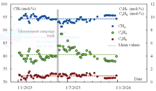
Figure 1.
Temporal evolution of the composition of the bunkered gas throughout 2023.
We note that the final samples of the year are more stable due to a different bunkering port. This figure shows that the fuel composition remained broadly stable, although the relative fluctuations in propane and ethane are more pronounced because of their low concentrations. No seasonal patterns or significant composition drifts are evident. The LNG used during the onboard campaign contained 94.14 mol-% methane, 3.96 mol-% ethane, and 1.26 mol-% propane, and the pilot fuel was a marine gas oil (MGO) with low sulfur level of 0.07 m-%. We report these values in Table 1, including both Lower Heating Value (LHV) and Methane Number (MN). The table also presents the corresponding annual averages and coefficients of variance (COV), along with the values reported in the testbed EIAPP certification report. These results confirm that the LNG used during the week of emission measurements is representative of the annual fuel supply, with an MN = 78, slightly higher than the average one over the year (MN = 79.7).

Table 1.
Composition and key parameters of the LNG (Lower Heating Value, Methane Number).
When comparing the bunkering values to testbed LNG characteristics, it appears that the average methane number is lower than the MN = 85 reported during engine test bench certification. IMO does not prescribe a single standardized reference fuel for LNG-fueled engine bench tests in the same way that reference fuels exist for conventional fuels (e.g., ISO 8217 marine diesel). But the characteristics of the fuel used for the test are “to be determined and recorded” [16]. Low-pressure dual-fuel four-stroke engines require a methane number above MN > 70 [15], and some engine manufacturers even recommend MN > 80, although as noted by Kuczyński et al. [17], a significant portion of the liquefied natural gas available on the market does not meet this threshold. Despite this observation, the average methane number over the year remains close to 80, with limited variability.
Regarding the propulsion configuration, engines are directly connected to the propellers via a reduction gearbox. Propulsive power is modulated through a combined control of propeller pitch and engine rotation speed. Even though the engine speed varies between 465 and 600 revolutions per min (rpm) during the vessel’s operational life, the E2 cycle applicable to constant-speed propulsion engines is used for this engine’s certification. During regular operation, the vessel employs different propulsion modes. During maneuvering, the engine runs at a constant speed while power output is controlled by adjusting the propeller pitch. In contrast, during sea passages, the ship operates in “combinator mode”, where both the engine speed and propeller pitch are varied simultaneously according to a control map designed to optimize propulsive efficiency and, consequently, reduce fuel consumption and atmospheric emissions. This configuration differs from that of some large cruise ships, where the engines operate at constant speed and supply electricity to propulsion motors (PODs) via alternators. Two recent studies have been conducted on this Wärtsilä 46DF engine model in such diesel–electric, constant-speed configurations [12,13]. The evaluation of engine emission factors is typically performed at steady-state load points, with values and weighting factors defined by type-approval test cycles. For propulsion engines, the International Maritime Organization (IMO) prescribes the weightings applied to different load levels: 10%, 25%, 50%, 75%, and 100% engine load. Most studies focusing on LNG engine emission factors, therefore, target measurements near these nominal load points. However, onboard measurements during commercial operation often cannot reach 100% load. Furthermore, some recent investigations [7,12,18] include low-load conditions (around 10%), due to the known increase in emission factors at such loads and the anticipated regulatory changes to better account for this phenomenon, even though it might be difficult to achieve stable 10% under operational conditions. The NOx Technical Code [16] specifies the requirements for the five steady-state load points during engine bench testing: a duration of 10 min per load point, with a sampling frequency of 1 Hz and a coefficient of variance (COV) of engine load below 5%. This COV is defined as the ratio of the standard deviation to the mean engine load. For this study, conducted during commercial operations of the vessel and on a main propulsion engine, we requested the crew to perform engine load plateaus without targeting specific load values. During low-load operations in port environments, it was not possible to maintain prolonged plateaus; as a result, durations ranged from 5 to 10 min. This is illustrated in Figure 2, which shows the data recorded during the vessel’s departure from the Port of Bilbao, sailing to Rosslare (Ireland). The instrumentation used for this monitoring is presented in Figure 3. In Figure 2a, the vessel’s route is shown alongside engine load and the geographical locations of stabilized points (with point numbers P1 to P11, engine load values, and COV listed in the legend). In Figure 2b, synchronous recordings of engine load and methane concentration in the exhaust are presented, highlighting the 11 identified steady-state phases P1 to P11. As can be observed, methane slip concentration is strongly correlated with engine load, with significant peaks occurring during load reductions. Additionally, a brief gas trip (i.e., an automatic interruption of gas fuel supply that is triggered by the engine’s control system, usually to prevent damage or unsafe conditions) is visible between 19:00 and 20:00. During this event, the engine switched from LNG to MGO mode, the methane concentration dropped to zero before rising again, and the engine load fell below 40% before recovering. This recording shows that at low engine loads (points 1 to 3, corresponding to 32%, 45%, and 58% load), increasing the load results in a significant decrease in methane concentration. This is consistent with the well-known behavior of increased methane slip with decreasing load, at low engine loads. Between points 4 and 5 (75% to 86% load), the increase in load leads to a further decrease in exhaust methane concentration, whereas between points 6 and 7 (71% to 60% load), a decrease in load also leads to a decrease in methane concentration. While this may seem counterintuitive, Figure 4b reveals a coherent slight increase in the methane slip emission factor between 50% and 70% load, followed by a decrease beyond 70%.
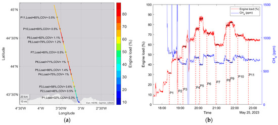
Figure 2.
Monitoring of a departure from the Port of Bilbao (Spain), (a) Ship trajectory colored by engine load; (b) Monitoring of engine load together with CH4 concentration in the exhaust.
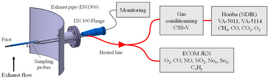
Figure 3.
Measurement setup on board the Salamanca.
During this onboard measurement campaign, we were able to carry out 16 h of recording and identify 31 measurement points with 10 min of stabilized engine load, as well as 51 points with measurement durations between 5 and 10 min. For all 82 points, the coefficient of variation (COV) of engine load remained below 5%. The corresponding details are summarized in Table 2. It can be observed that the COV of methane concentration—also measured at a 1 Hz frequency—is generally higher, yet the mean value remains below 5%, indicating good emission stability. Among the 82 measurement points, the maximum observed COV for CH4 is 12.7%. However, only seven points exceed a COV of 5%, all of which correspond to engine loads below 45%.
Table 2.
Analysis of the mean, maximum, and COV values for the engine load and the CH4 concentration at the averaging points of the measurements.
2.2. Emission Measurements
Emission measurements were conducted in the exhaust line of the port-side main engine (ME2). For this purpose, a DN100 access port was installed prior to the measurement campaign on the upper deck, as close as possible to the atmospheric exhaust outlet. On this flange, two heated (180 °C) sampling lines were installed—one for particle sampling and one for gas-phase analysis. A Pitot-type velocity probe was used to measure both the gas velocity and temperature along the exhaust axis, allowing a direct estimation of the exhaust mass flow rate. Methane (CH4), carbon monoxide (CO), and carbon dioxide (CO2) concentrations were quantified directly in the raw exhaust using a conventional Non-Dispersive Infrared (NDIR) analyzer (VA-5000, HORIBA, Tokyo, Japan). Additionally, nitrogen oxides (NOx) emissions were measured with a flue gas analyzer (J2KN, ECOM, Iserlohn, Germany) equipped with electrochemical sensors. The complete setup of the gaseous sampling system and measurement instruments is illustrated in Figure 3.
To convert methane concentrations into emission factors expressed in grams per kilowatt-hour, it is necessary to determine both the exhaust gas flow rate and the engine power output. The calculation of the power delivered by the engine is based on a torque measurement sensor taken directly at the engine output shaft. Using simultaneous recordings of rotational speed and torque, the engine power during the tests was calculated as a function of load (see Figure 5a, below). The deviation between the calculated power values and those from the EIAPP data remains below 1.3%, with this maximum difference observed at 75% engine load. The exhaust flow was estimated using the carbon balance method, as defined in the NOx Technical Code, based on exhaust gas concentrations and the measured fuel flow rates for both LNG and pilot fuel. As with engine power, the fuel consumption data required for this carbon balance approach were recorded on board and retrieved by the ship operator from the engine manufacturer’s monitoring system. Analysis of these datasets confirmed that both LNG consumption and delivered engine power scale linearly with engine load and are consistent with the values reported in the engines’ EIAPP (Engine International Air Pollution Prevention) certificate (see Figure 5b for the LNG consumption, below). The gas flow meter used for flow measurement is a high precision Coriolis-type device (Proline Promass F500, Endress+Hauser AG, Reinach, Switzerland). As shown in Figure 5b, the discrepancy between the measured flow rates and those obtained during engine bench testing for EIAPP certification is minimal. The maximum relative deviation observed is 3.5% at 25% engine load.
2.3. Engine Load Monitoring Method
Based on the emission factors of an engine and its operational profile, represented by the engine load as a function of time, it is possible to calculate the yearly average equivalent slip coefficient, Cslip, over a one-year reference period. The objective is that this coefficient of slip, when applied to the actual fuel mass consumed during the reference period, accurately reflects the effective atmospheric release due to methane slip in the exhaust over that same period. This approach, commonly referred to as ELM (Engine Load Monitoring), is currently under discussion, and a working document submitted to MEPC 83 outlines the calculation procedure to be followed in determining this equivalent slip coefficient.
We present below the main steps used to compute the slip coefficient Cslip, using the ELM method. This approach considers the actual engine load during operation, instead of relying on the predefined weighting factors described in the NOx Technical Code and combines it with CH4 emission factors to derive more representative emission estimates.
- (a)
- Emission values at different engine loads.
Emission values at specific reference engine loads are derived from CH4 emission measurements obtained through test-bed or onboard campaigns. The reference loads are 10%, 25%, 50%, 75%, and 100%. For onboard measurements, the 100% can be replaced by a lower load; however, it cannot be lower than 85%. For load points between two measured values, emission values are determined by linear interpolation between the nearest measured points above and below the target load. For load points outside the measured range (i.e., below the lowest or above the highest measured load), emission values are estimated based on available data. The following estimation approaches may be applied, depending on the range and distribution of measured points:
- Linear extrapolation using the two closest points if the lowest measured load is ≤ 10%;
- Polynomial interpolation using all measured points if the lowest measured load is 25%;
- Linear extrapolation using the two closest points if the highest measured load is ≥ 90%;
- Polynomial interpolation using all measured points if the highest measured load is 75%.
- (b)
- Load monitoring.
The load of the engine considered must be continuously monitored. Engine load data should be averaged over 30 min intervals, excluding periods of zero load or operation on diesel fuel.
- (c)
- Calculations.
Emission values for corresponding engine loads are calculated based on verified measurements, expressed in units of g/g fuel (i.e., as a percentage of the fuel mass consumed by the engine). The annual methane slip coefficient Cslip (g/g fuel) is determined using the following procedure:
- The total fuel mass (in kg) consumed during each 30 min interval is calculated using data from the fuel flow meter.
- The emission factor (as a percentage) corresponding to the average engine load during the interval is obtained from the measurement data, as outlined in Point 1.
- The methane emission mass (in kg) for the interval is computed by multiplying the total fuel mass of the 30 min interval by the emission factor.
- The annual weighted slip coefficient (Cslip) for the whole monitoring period is achieved by dividing the total emission (kg) over the reporting period by the total fuel mass (in kg) consumed during the same period.
The procedure described above defines the analysis period as being divided into 30 min intervals. In this study, we propose varying the length of these intervals. Furthermore, the procedure was originally designed to produce an annual emission balance, but it can also be applied to shorter analysis periods. Since the Salamanca operates on a weekly rotation schedule, we applied the procedure over one-week periods to calculate a weekly slip coefficient Cslip,week and to investigate the variability of methane emissions to the atmosphere.
3. Results
3.1. Methane Emission Factor
The average methane concentrations obtained at stabilized engine loads were converted into emission factors expressed in grams per kilowatt-hour and are presented in Figure 4. Alongside these results, data from two other studies conducted on Wärtsilä 46DF engines are shown: one by Kuittinen et al. [12] and another by Sagot et al. [13]. As is often the case, Kuittinen et al. [12] performed measurements at five reference engine load points, whereas the study by Sagot et al. was conducted during sea trials of a vessel nearing completion, resulting in more varied engine loads across the measurement points. We observe that the emission factor levels measured in this study on the Salamanca are consistent with those reported in these two earlier investigations, both conducted on similar engines installed on large cruise ships with diesel–electric propulsion architecture. However, we identify a marked discontinuity in the distribution of the emission factors around 40% engine load (grey area). This discontinuity is linked to the propulsion chain architecture and the use of the combined operating mode and is the subject of a detailed analysis in Section 3.2.
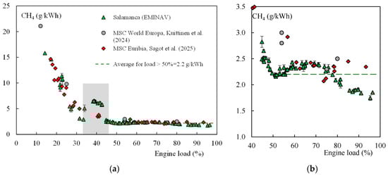
Figure 4.
CH4 emission factor as a function of engine load. Comparison with previous onboard measurement of 46DF by Kuittinen et al. [12] and Sagot et al. [13]: (a) Full load range; (b) Zoom on the 40–100% load range.
In the second part of the figure (Figure 4b), we provide a zoomed view of the engine load range from 40% to 100%. Within this range, 66 measurement points are shown, all having a coefficient of variation (COV) for both engine load and methane concentration below 5% (with average COVs of 1.3% for engine load and 1.6% for methane). Among these, 29 points correspond to 10 min measurements, and the remainder range between 5 and 10 min in duration. These measurements were conducted across several different days, and the low dispersion of the data points within this load range demonstrates good repeatability of the entire instrumentation chain and post-processing methodology. Finally, the discontinuity observed in the emission factor curve and revealed through continuous monitoring of emissions over a wide engine load range is further explored in detail in the following subsection.
3.2. Analyses of the Non Linearity in the Emission Factor Curve
The discontinuity in emission factors as a function of engine load (Figure 4) is quite pronounced, and we sought to explain this phenomenon. When plotting the exhaust mass flow as a function of the engine load (Figure 5a, below), a clear discontinuity can also be observed near 40% engine load. This discontinuity is confirmed by two completely independent methods: one based on direct exhaust flow measurement using a Pitot tube, and the other based on the fuel flow measurement and the exhaust gas composition analysis. These two determinations are highly consistent with each other, as well as with the measurements reported in the technical file accompanying the engine’s EIAPP certificate of the ME2 engine. This technical file provides detailed technical values such as the power, fuel flow, and exhaust gas flow as a function of the engine load for the test cycle measurement points.
On Figure 5b, we present an analysis of the high-frequency recordings (at Hertz level) during the measurement week, specifically for the boost pressure and the LNG flow, that further confirms the discontinuity, clearly in the boost pressure curve, and to a lesser extent in the gas consumption curve of engine ME2.
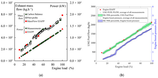
Figure 5.
(a) Exhaust mass flow and power as a function of engine load, by different methods; (b) LNG fuel flow and boost pressure as a function of engine load.
Using the air and fuel flow rates, the intake air/fuel ratio was calculated and are reported in Figure 6. Once again, a marked discontinuity appears in the same engine load range.
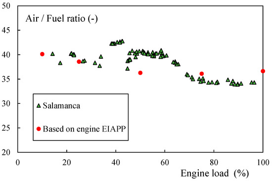
Figure 6.
Evolution of the air/fuel mass flow ratio with engine load.
This analysis confirms that the observed discontinuity in methane slip emission factors is not a measurement artifact but rather linked to variations in the air/fuel ratio, which is the most influential parameter affecting incomplete combustion [19]. In fact, the same discontinuity is observed across all gaseous concentrations expressed in grams per kilowatt-hour, including O2, CO, CO2, and NOx. Discussions with the ship operator’s engineering team suggest that this phenomenon is likely related to the use of the combinator mode, which controls propulsion by adjusting both engine speed and propeller pitch to optimize efficiency. At lower engine rotation speed, there is a risk of surge in the turbocharger’s air supply turbine, which can lead to damage. To prevent this, the engine control system actuates an air bypass valve, which affects the air/fuel ratio. However, in the absence of detailed data on the engine’s control logic, this remains a working hypothesis that would require further verification. As we have shown, these variations in the air/fuel ratio also have a direct impact on the methane slip emission factor, although the increase remains limited and occurs within a relatively narrow engine load range. This analysis confirms the relevance of conducting exploratory measurements beyond the specific load points defined in the engine’s EIAPP certificate, particularly in the context of a direct mechanical propulsion architecture.
3.3. Application of the Engine Load Monitoring Method for the Calculation of the Annual Methane Slip Coefficient
The analysis presented here aims to align as closely as possible with the ELM (Engine Load Monitoring) procedure described above (see Section 2.3), using on-board emission factor measurements and the engine load profile of Salamanca for the year 2023.
The first step is to construct an interpolation between the measurement points. Since we have multiple data points, we defined reference points based on the average of the measurements, which are then used to construct linear or quadratic interpolations. According to the proposed procedure, for low engine loads, extrapolation beyond the lowest measured load point must be polynomial to avoid underestimation by the interpolated emission factor. We opted for a conservative approach by maximizing the emission factor relative to measured points: the observed discontinuity is, thus, accounted for, even if it is not explicitly addressed in the discussed procedure. Emission factors are expressed either in grams per kilowatt-hour or as a slip coefficient , expressed as g/g fuel (i.e., as a percentage of the fuel mass consumed by the engine). It is worth noting (see Figure 7 below) that the proposed quadratic interpolation is consistent with the point measured at 12% load on an equivalent engine by Kuittinen et al. [12].
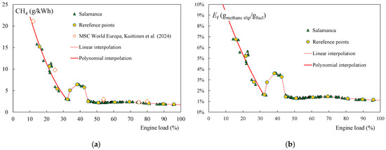
Figure 7.
CH4 emission factor as a function of engine load. (a) Emission factor (g.kW.h−1), with data from Kuittinen et al. [12]. (b) Slip coefficient (%) as a function of engine load.
The procedure then requires averaging the recorded engine load in 30 min intervals, excluding periods when the engine load is zero. This step is illustrated in Figure 8a. The automated processing detects engine start-up and shutdown and calculates average loads over 30 min intervals, the last interval being truncated. On this sequence, we observe that the load of the starboard engine ME1 increases significantly just after 16:00, corresponding to the shutdown of ME2 (the engine considered in this study). Shutting down ME2 allows the navigation phase to continue with ME1 operating at higher load, while the second engine is turned off.

Figure 8.
30 min engine load averaging procedure. (a) Illustration of the 30 min period averaging for ME2. (b) Yearly (2023) ME2 load distribution, and impact of averaging on distribution.
This automated processing was applied to a full year of recordings, totaling 6980 h of engine operation, indicating that the engine was in use about 80% of the time throughout the year 2023. Figure 8b shows the engine load distribution resulting from this analysis, with and without 30 min averaging. The averaging procedure smooths the peak observed around 8% load, which corresponds to idle phases during engine start-up at berth, clearly visible in Figure 8a just before 11:00. The average relative deviation between the two distributions for engine loads below 30% is 63%, while it is only 12% for loads between 30% and 100%. Given the operational profile of the Salamanca, the 30 min averaging has a minimal impact on the annual engine load distribution, except at low engine loads.
Based on this procedure of dividing the operational period into n intervals of 30 min (or shorter for the final segments of navigation), each identified by its index, i, the average methane slip coefficient, , over the entire analysis period can be evaluated, defined by dividing the total emission (kg) by the total fuel mass (kg) consumed:
with being the average engine load during interval, i, and are, respectively, the fuel mass flow rate (kg·s−1) and the emission factor (%), both evaluated at the average load, , and is the duration of interval, i.
By applying this calculation method over the full year 2023, the resulting coefficient is 1.57%. This value, obtained using the so-called Engine Load Monitoring (ELM) methodology, is lower than the default values of 3.1% and 3.5% specified by the FuelEU Maritime regulation [11] and IMO LCA guidelines [10].
3.4. Investigation on the Parameters of the ELM Procedure, and Discussion
As previously shown in Figure 8b, the 30 min averaging procedure alters the engine load distribution, with a smoothing effect at low loads. By varying the reference averaging period, it is possible to assess, for the same emission factor curve, the impact on the annual coefficient. The results presented in Figure 9 show that the increase associated with this averaging duration is extremely small. For a 10 min averaging period, the value is 1.55%, and close to 1.54% with no averaging at all. Therefore, applying the 30 min interval ELM procedure does not underestimate this vessel’s methane slip emissions.
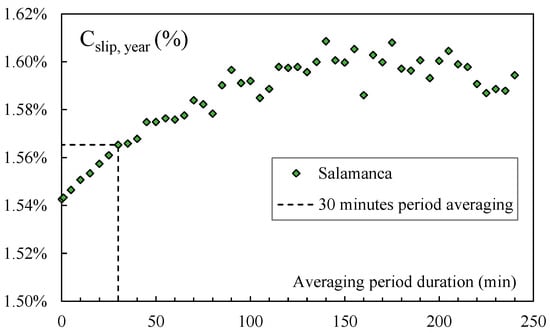
Figure 9.
Evolution of the yearly slip coefficient, Cslip, with the averaging period duration.
We applied the ELM approach over a full year, as it is intended to provide shipowners with an annual emission assessment of a vessel. However, it can also be applied to shorter reference periods. Since this vessel operates regular routes on a fixed weekly schedule that brings it back to Cherbourg (France) once a week for crew change, we calculated the average coefficient on a weekly basis for each of the 51 full weeks within year 2023. This allowed us to examine the impact on the weekly average emission factor of the variability in the operational profile that is related to weather conditions, tidal currents, and various uncertainties at sea and during port calls. Figure 10 shows the distribution of the obtained for the 51 weeks. Seven weeks stand out, with values exceeding 1.65%. Data analysis revealed that these correspond to the final weeks of the year, during which the vessel’s operational profile and destinations have changed within the weekly schedule, including low-speed nighttime navigation and, thus, low engine load conditions. If these seven weeks are excluded, it becomes clear that under a stable weekly schedule, the variability of remains limited, with less than 15% between the minimum and maximum observed values of . This analysis finally illustrates how the ELM approach can also support the optimization of operational profiles to reduce methane slip emissions.
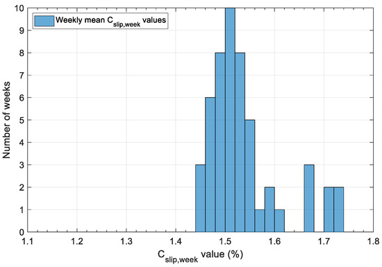
Figure 10.
Distribution of the weekly average slip coefficient Cslip,week.
Two average slip coefficient values were evaluated in recent studies by Kuittinen et al. [12] and Sagot et al. [13], both of which reported values of 1.7%. In both cases, the studies concerned cruise ships with diesel–electric propulsion architecture. The value of 1.57% for the average Cslip coefficient obtained in this study is slightly lower than those reported in the two referenced studies, primarily due to the vessel’s specific operational profile, which includes a very limited proportion of time spent at low engine loads. Furthermore, we verified that the load distribution between the vessel’s two engines is perfectly balanced, as are the discontinuities observed in the fuel consumption and turbocharging pressure curves. As a result, the approach developed and applied to one engine is fully transferable to both engines installed on the ship.
The starting point of the methodology developed in this study is the methane slip emission factor curve as a function of engine load, which was directly measured onboard. The procedures for defining these emission factors are still under discussion, particularly regarding the instrumentation used. The recent inter-comparison study by Lehtoranta et al. [18] is especially valuable in this context, highlighting the practical challenges of implementing measurement systems, especially under onboard conditions. This is notably the case with FID (Flame Ionization Detection) systems, which require hydrogen cylinders, posing safety concerns on passenger vessels. As emphasized in the recent report by Moutik and Benedetti [20], which provides a comprehensive overview of methodologies for onboard measurement campaigns, producing reliable emission factors in operational conditions remains both a technical and logistical challenge. This explains why, since the study conducted by Anderson et al. ([3], 2015), fewer than ten studies have been carried out on LNG-powered ships. However, this study is the third measurement campaign carried out on a Wärtsilä 46DF engines, and our measurement results show a remarkable level of consistency with the two previous studies [12,13] conducted in very different measurement conditions.
4. Conclusions
By combining engine emission factors with the Engine Load Monitoring (ELM) methodology used in this study, it becomes possible to evaluate the actual methane emissions of a vessel over a given operational period. The application of this calculation method over the full year 2023 on the ROPAX vessel Salamanca resulted in an exhaust methane slip Cslip coefficient of 1.57%, a value that is particularly low. When scaled to a fleet level, this approach enables the integration of real operational profiles into the assessment of actual atmospheric emissions. In the current context of evolving regulations and the monetization of methane emissions [18], the accurate quantification of real emissions is becoming essential. Improved consideration of ships’ actual emissions will make regulatory frameworks more effective and potentially more incentive-based, thus encouraging both the deployment of emission reduction technologies at the engine level and the optimization of operational profiles, for example, through the hybridization of propulsion systems.
Author Contributions
Conceptualization, B.S.; Formal analysis, B.S. and R.D.; Funding acquisition, B.S.; Investigation, B.S. and R.D.; Methodology, B.S. and R.D.; Project administration, B.S. and A.J.; Resources, B.S.; Validation, B.S.; Writing—original draft, B.S., R.D., R.M., A.V. and A.J.; Writing—review and editing, B.S., R.D., R.M., A.V. and A.J. All authors have read and agreed to the published version of the manuscript.
Funding
This research was funded by the French project ADEME AQACIA EMINAV, grant number 2266D0003.
Data Availability Statement
All the data relevant to interpretation of results are available in the article.
Acknowledgments
The authors are grateful to ADEME for their financial and operational support and to all the crew members of the Salamanca, who welcomed and assisted us onboard this vessel. We would also like to thank David Perez and Franck Faux for their support and assistance in contributing to the preparation and realization of the measurement campaigns, and in designing and integrating the sampling system. We would like to thank Vincent Coquen and Bertrand Crispils from Brittany Ferries for their valuable contribution to the measurement campaigns organization, project coordination with the crews, and data retrieval.
Conflicts of Interest
The authors declare no conflicts of interest.
Abbreviations
The following abbreviations are used in this manuscript:
| COV | Coefficient Of Variance, defined as the ratio of the standard deviation to the mean |
| EIAPP | Engine International Air Pollution Prevention |
| ELM | Engine Load Monitoring |
| GFI | Greenhouse gas Fuel Intensity |
| GHG | Greenhouse gas |
| GWP | Global Warming Potential |
| HFO | Heavy Fuel Oil |
| IMO | International Maritime Organization |
| LNG | Liquefied Natural Gas |
| LHV | Lower Heating Value |
| LCA | Life Cycle Assessment |
| ME2 | Main Engine 2 |
| MGO | Marine Gas Oil |
| NDIR | Non-Dispersive InfraRed |
References
- Balcombe, P.; Staffell, I.; Kerdan, I.G.; Speirs, J.F.; Brandon, N.P.; Hawkes, A.D. How Can LNG-Fuelled Ships Meet Decarbonisation Targets? An Environmental and Economic Analysis. Energy 2021, 227, 120462. [Google Scholar] [CrossRef]
- Corbin, J.C.; Peng, W.; Yang, J.; Sommer, D.E.; Trivanovic, U.; Kirchen, P.; Miller, J.W.; Rogak, S.; Cocker, D.R.; Smallwood, G.J.; et al. Characterization of Particulate Matter Emitted by a Marine Engine Operated with Liquefied Natural Gas and Diesel Fuels. Atmos. Environ. 2020, 220, 117030. [Google Scholar] [CrossRef]
- Anderson, M.; Salo, K.; Fridell, E. Particle- and Gaseous Emissions from an LNG Powered Ship. Environ. Sci. Technol. 2015, 49, 12568–12575. [Google Scholar] [CrossRef] [PubMed]
- Peng, W.; Yang, J.; Corbin, J.; Trivanovic, U.; Lobo, P.; Kirchen, P.; Rogak, S.; Gagné, S.; Miller, J.W.; Cocker, D. Comprehensive Analysis of the Air Quality Impacts of Switching a Marine Vessel from Diesel Fuel to Natural Gas. Environ. Pollut. 2020, 266, 115404. [Google Scholar] [CrossRef] [PubMed]
- Lehtoranta, K.; Aakko-Saksa, P.; Murtonen, T.; Vesala, H.; Ntziachristos, L.; Rönkkö, T.; Karjalainen, P.; Kuittinen, N.; Timonen, H. Particulate mass and nonvolatile particle number emissions from marine engines using low-sulfur fuels, natural gas, or scrubbers. Environ. Sci. Technol. 2019, 53, 3315–3322. [Google Scholar] [CrossRef] [PubMed]
- Aakko-Saksa, P.T.; Lehtoranta, K.; Kuittinen, N.; Järvinen, A.; Jalkanen, J.P.; Johnson, K.; Jung, H.; Ntziachristos, L.; Gagné, S.; Takahashi, C.; et al. Reduction in Greenhouse Gas and Other Emissions from Ship Engines: Current Trends and Future Options. Prog. Energy Combust. Sci. 2023, 94, 101055. [Google Scholar] [CrossRef]
- Lehtoranta, K.; Kuittinen, N.; Vesala, H.; Koponen, P. Methane Emissions from a State-of-the-Art LNG-Powered Vessel. Atmosphere 2023, 14, 825. [Google Scholar] [CrossRef]
- Kuittinen, N.; Heikkilä, M.; Lehtoranta, K. Review of Methane Slip from LNG Engines; Green Ray Project. Deliverable D1.1; GREEN RAY, EU: Brussels, Belgium, 2023. [Google Scholar]
- Stenersen, D.; Thonstad, O. GHG and NOx Emissions from Gas Fuelled Engines; Mapping, Verification, Reduction Technologies; SINTEF Ocean AS: Trondheim, Norway, 2017; pp. 1–52. [Google Scholar]
- MEPC 81-2024 GUIDELINES ON LIFE CYCLE GHG INTENSITY OF MARINE FUELS (2024 LCA GUIDELINES). Available online: https://wwwcdn.imo.org/localresources/en/OurWork/Environment/Documents/annex/MEPC 81/Annex 10.pdf (accessed on 25 February 2025).
- FuelEU Maritime. Regulation (EU) 2023 of the European Parliament and of the Council on the Use of Renewable and Low-Carbon Fuels in Maritime Transport, and Amending Directive 2009/16/EC, 2023. Available online: https://eur-lex.europa.eu/eli/reg/2023/1805/oj (accessed on 27 February 2025).
- Kuittinen, N.; Koponen, P.; Vesala, H.; Lehtoranta, K. Methane Slip and Other Emissions from Newbuild LNG Engine under Real-World Operation of a State-of-the Art Cruise Ship. Atmos. Environ. X 2024, 23, 100285. [Google Scholar] [CrossRef]
- Sagot, B.; Giraudier, G.; Decuniac, F.; Lefebvre, L.; Miquel, A.; Thomas, A. On-Board Measurement of Emissions on a Dual Fuel LNG Powered Cruise Ship: A Sea Trial Study. Atmos. Environ. X 2025, 25, 100313. [Google Scholar] [CrossRef]
- Balcombe, P.; Heggo, D.A.; Harrison, M. Total Methane and CO2 Emissions from Liquefied Natural Gas Carrier Ships: The First Primary Measurements. Environ. Sci. Technol. 2022, 56, 9632–9640. [Google Scholar] [CrossRef] [PubMed]
- Ushakov, S.; Stenersen, D.; Einang, P.M. Methane Slip from Gas Fuelled Ships: A Comprehensive Summary Based on Measurement Data. J. Mar. Sci. Technol. 2019, 24, 1308–1325. [Google Scholar] [CrossRef]
- MEPC, IMO Resolution. 177 (58), 2008. Amendments to the Technical Code on Control of Emission of Nitrogen Oxides from Marine Diesel Engines (NOx Technical Code 2008) IMO London. Available online: https://wwwcdn.imo.org/localresources/en/OurWork/Environment/Documents/177(58).pdf (accessed on 27 February 2025).
- Kuczyński, S.; Łaciak, M.; Szurlej, A.; Włodek, T. Impact of Liquefied Natural Gas Composition Changes on Methane Number as a Fuel Quality Requirement. Energies 2020, 13, 5060. [Google Scholar] [CrossRef]
- Lehtoranta, K.; Vesala, H.; Flygare, N.; Kuittinen, N.; Apilainen, A.-R. Measuring Methane Slip from LNG Engines with Different Devices. J. Mar. Sci. Eng. 2025, 13, 890. [Google Scholar] [CrossRef]
- Rochussen, J.; Jaeger, N.S.B.; Penner, H.; Khan, A.; Kirchen, P. Development and Demonstration of Strategies for GHG and Methane Slip Reduction from Dual-Fuel Natural Gas Coastal Vessels. Fuel 2023, 349, 128433. [Google Scholar] [CrossRef]
- Moutik, B.; Benedetti, G. Onboard Methane Slip Emissions Measurement: Practical Insights and Industry Lessons Learned; SGMF: London, UK, 2025. [Google Scholar]
Disclaimer/Publisher’s Note: The statements, opinions and data contained in all publications are solely those of the individual author(s) and contributor(s) and not of MDPI and/or the editor(s). MDPI and/or the editor(s) disclaim responsibility for any injury to people or property resulting from any ideas, methods, instructions or products referred to in the content. |
© 2025 by the authors. Licensee MDPI, Basel, Switzerland. This article is an open access article distributed under the terms and conditions of the Creative Commons Attribution (CC BY) license (https://creativecommons.org/licenses/by/4.0/).