Power Assessment and Performance Comparison of Wind Turbines Driven by Multivariate Environmental Factors

Abstract

The increasing deployment of turbines installed offshore is critical for sustainable energy development, yet accurate performance assessment remains challenging due to complex environmental influences, diverse turbine control strategies, and issues with data quality. Traditional performance metrics and power curve models often fail to provide reliable cross-turbine comparisons because they neglect multivariate environmental factors and turbine-specific biases. To address these limitations, this study develops a novel multivariate environmental factor-driven power assessment framework employing segmented long short-term memory (LSTM) models. A hybrid data cleaning method, combining bidirectional quartile analysis with the power curtailment detection, is proposed to effectively identify outliers, including subtle anomalies within typical data ranges. Samples are segmented based on rated wind speed to reflect differences in control strategies, and turbine-specific operational parameters are excluded to ensure unbiased comparisons among turbines. The proposed method achieves substantial improvements in predictive accuracy, with decreases of 9.39% in mean absolute error (MAE) and 11.75% in root mean square error (RMSE), compared to conventional binning approaches. When applied to three 5.5 MW offshore wind turbines, the proposed method reveals significant differences among the units. Turbine A demonstrates the highest performance, while turbines B and C exhibit reductions of 14.35% and 8.29%, respectively. Operational state analysis shows that turbine B experiences substantially longer maintenance durations, indicating severe faults that adversely affect its operational reliability and power output. These findings provide valuable insights for maintenance prioritization and performance benchmarking among wind turbines.

1. Introduction

With the rapid depletion of fossil fuels and their nonrenewable nature, there is an urgent need to accelerate the advancement of renewable energy technologies [1]. Due to its low emissions and environmental friendliness, wind power is considered a key strategic option for the sustainable development of electricity. According to the International Energy Agency (IEA), the global share of wind power has continued to rise and comprised approximately 29% of new renewable energy installations in 2023 [2]. Compared to onshore wind farms, offshore wind energy offers enhanced potential for large-capacity wind turbines due to more abundant and stable wind resources [3]. Consequently, offshore wind is widely recognized as a pivotal contributor to achieving long-term global climate targets. By the end of 2022, the combined capacity of onshore wind farms installed globally reached 841.9 gigawatts, while offshore wind power installations totaled 64.3 gigawatts. Throughout that year, the wind energy sector saw an expansion of 77.6 gigawatts in new capacity additions worldwide [4]. Wind turbines are primarily classified based on their axis of rotation into horizontal-axis wind turbines (HAWTs) and vertical-axis wind turbines (VAWTs) [5]. Among these, HAWTs have become the mainstream choice for offshore wind power due to their higher efficiency and scalability. To enhance the performance and cost-effectiveness of wind turbines, various optimization methods have been employed, including aerodynamic optimization, structural design improvements, and control strategy refinement, often utilizing advanced techniques such as computational fluid dynamics (CFD) and multi-objective optimization [6].

Although offshore wind offers many benefits, operating turbines offshore encounters considerable challenges because of the requirements for remote connectivity and the harsh weather conditions [7]. Accurately assessing turbine performance anomalies and implementing scientifically sound maintenance or technological upgrades have become critical to enhancing power generation capacity. Current industry practices rely on metrics such as energy yield, capacity factor, power curve analysis, and multivariate power evaluation for turbine performance assessment [8]. Energy yield functions as a foundational metric that directly reflects the actual power generation of a turbine over a given period. It quantifies the total electrical energy produced by the turbine within a specified timeframe, and this energy is typically expressed in megawatt-hours (MWh) [9]. The capacity factor, which represents the proportion of actual energy generated compared to the maximum possible output, quantifies turbine utilization efficiency over a given period [10]. It serves as a key indicator to assess how effectively a turbine converts available wind resources into electrical energy. A higher capacity factor signifies better performance and indicates that the turbine operates closer to its full potential, which is critical for planning, investment decisions, and comparing different wind energy projects. However, both metrics are influenced by multiple factors, including operational hours, failure rates, and environmental conditions, limiting their ability to comprehensively evaluate turbine performance.

While power curves assess turbine performance across wind speeds, they rely solely on wind speed data, neglecting the combined effects of variables such as wind direction and temperature. This omission introduces environmental interference during cross-turbine comparisons. To address this, multivariate power assessment methods have emerged as essential tools [11,12]. These methods not only improve accuracy in real-world operational assessments but also provide robust data support for fault diagnosis, performance optimization, and maintenance strategies [13]. A study investigated the impact of critical environmental factors on turbine power output [14]. The findings revealed that turbulence intensity (TI) below 10% has a limited effect on power generation. However, as turbulence intensity increases, power output at wind speed near the cut-in threshold shows significant improvement, while near the rated wind speeds, it tends to decline. Astolfi et al. [15] proposed a multivariate wind turbine power curve analysis method, incorporating environmental and operational parameters as inputs to data-driven models. By leveraging SCADA data alongside artificial intelligence and statistical techniques, this approach improves accuracy under non-steady-state conditions. Guo et al. [16] highlighted limitations in the IEC-61400-12-1 [17] standard’s binned power curve modeling and analyzed multiple factors affecting wind energy capture and turbine power output. To overcome the limitations of traditional wind turbine power curve (WTPC) approaches for modeling the complex nonlinear connection between wind speed and power output, Mushtaq et al. [18] developed a multivariate model, demonstrating tighter error distribution around zero compared to single-variable approaches. Wang et al. [19] established multivariate power assessment models using backpropagation neural networks (BPNNs) and support vector machines (SVMs) after preprocessing and anomaly detection of SCADA data. These models outperformed conventional power curve models in metrics such as MAE and RMSE. Addressing short-term autocorrelation in environmental parameters, Qiao et al. [20] proposed a multivariate power curve modeling method incorporating segmented control differences and short-term autocorrelation for cross-turbine performance comparison. Despite employing long short-term memory (LSTM) and gated recurrent unit (GRU) architectures, their models fell short of the baseline binning technique. The underperformance might be attributed to the lack of hyperparameter optimization, which is crucial for the effectiveness of complex neural network models [21].

In multivariate power assessment studies, key operational factors like rotor speed and pitch angle are often included as inputs to enhance single-turbine accuracy for long-term health monitoring [22,23]. However, in cross-turbine comparisons, these parameters introduce turbine-specific biases due to variations in control strategies and maintenance states, compromising objective assessment of environmental impacts. Therefore, standardized environmental features should serve as unified inputs to quantify external influences and ensure equitable comparisons.

To address cross-turbine performance analysis needs, this study proposes a novel multivariate environmental factor-driven power assessment framework for wind turbines. Initially, SCADA data are cleaned by filtering out discontinuous power generation records through operational codes. Subsequently, abnormal values are identified using a power curtailment detection algorithm combined with the bidirectional quartile method. Based on the control strategies, segmented LSTM models are constructed, and hyperparameters are optimized accordingly via grid search. Finally, by inputting unified environmental feature samples, the power generation performance of different wind turbines is compared. The principal contributions and unique features of this work are summarized as follows:

• A hybrid data cleaning approach is developed based on the bidirectional quartile method, with the incorporation of power curtailment detection. This method improves the identification of outliers in typical data distribution areas.
• Taking into account the differences between maximum power point tracking (MPPT) and constant power control approaches for variable-speed, variable-pitch wind turbines, the rated wind speed is used as the segmentation reference value to construct multivariable environmental factor samples for training a segmented LSTM model. The sample features are constructed without involving turbine-specific parameters (such as rotor speed, pitch angle, etc.), enabling the samples to serve as a unified input for comparing the power output of different turbines.
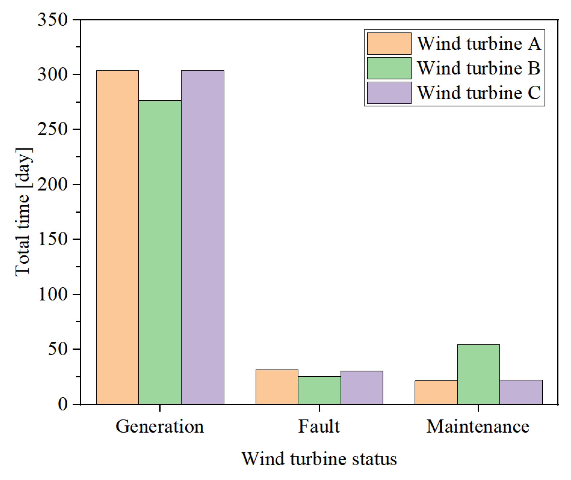
• By applying the proposed method to a full year of SCADA data, a comparative analysis of the power generation performance of three 5.5 MW offshore wind turbines is conducted. Furthermore, the results are compared with their annual power output, fault occurrences, and total maintenance time, thereby enriching the perspective on turbine performance assessment.

2. Methods

This section presents the methodological approaches involved in the proposed technical framework, including data cleaning, variations in wind turbine control strategies across different wind speed regimes, an LSTM-based machine learning model, and environmental feature selection.

2.1. Data Cleaning

Samples collected at 10 min intervals from the SCADA system were filtered to exclude non-continuous power generation states based on the unit operation codes. Then, the following algorithms identified samples under power curtailment conditions as well as abnormal samples.

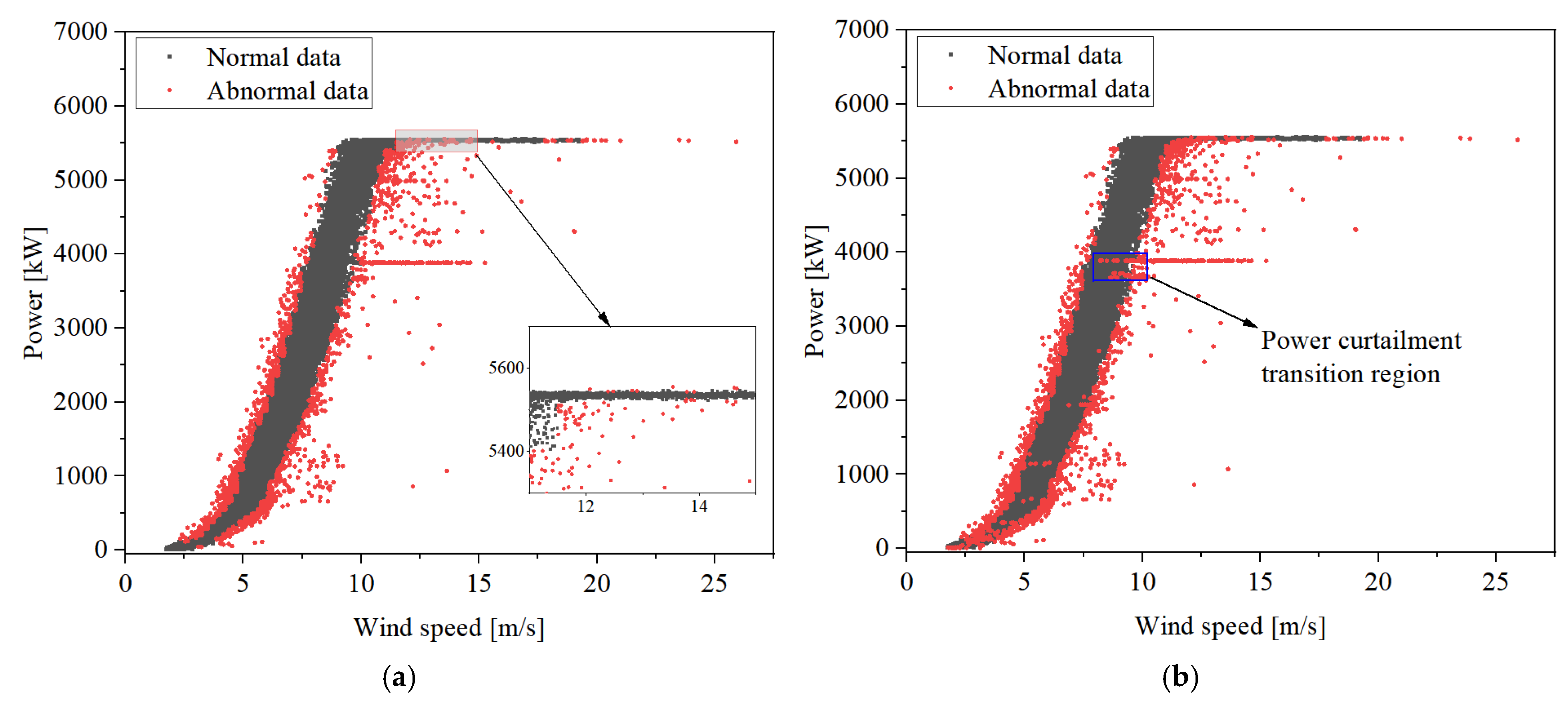
2.1.1. Power Curtailment Detection Algorithm

In handling a large dataset of accumulated power curtailment samples, the spatial distribution features of curtailed power data clustered within the transition region closely resemble those of normal data. As a result, normal data can be easily misclassified and removed, while the stacked power curtailment data may be overlooked. This misclassification negatively impacts the accuracy of multivariate measurable wind turbine curve models as well as turbine-level wind energy performance evaluations. Based on the time-series power data from the wind turbine SCADA system, a dynamically stability-driven curtailment state identification algorithm was proposed. For each power data point, an observation window containing the current point and the subsequent 6 consecutive samples was constructed. The standard deviation of the power values within the window was calculated. When the following conditions were simultaneously met, the time instant t was determined to be in a curtailment state:

$$\left\{\begin{array}{l}{\sigma }_t\le {\tau }_{\sigma }\\ P_t\le \phi P_{rated}\end{array}\right.,$$

(1)

where ${\sigma }_t$ is the standard deviation of the power within the window, ${\tau }_{\sigma }$ is a dynamic threshold determined through statistical analysis of historical data, P_t is the power at time t, P_rated is the rated power of the turbine, and $\phi$ is a proportional coefficient, typically set to 0.9 [20] or appropriately adjusted according to actual conditions.

2.1.2. Bidirectional Quartile Method

This study utilized a bidirectional quartile method to preprocess scattered anomalous data, predominantly represented by points distant from the typical wind power range. The term “bidirectional” refers to sequentially binning the data along two dimensions: wind speed and power. Within each bin, the quartile method was applied to identify and remove outliers [24]. This approach determines the data distribution through quartile calculation and utilizes the interquartile range (IQR) to identify outliers. The IQR is defined as follows:

$$IQR=Q3-Q1,$$

(2)

where Q1 represents the first quartile and Q3 the third quartile. A data point x_i is deemed normal if it falls within the range:

$$x_i\in \left[Q1-1.5\times IQR,Q3+1.5\times IQR\right].$$

(3)

Points that fall outside this boundary are categorized as outliers. Statistical bounds are clipped to the physical range when necessary.

2.2. Data Classification

Variable-speed, variable-pitch wind turbines are the mainstream models in the current wind power generation field. The main reasons include that variable-speed operation allows the turbine’s rotational speed to adapt to the wind speed, thereby maximizing wind energy capture and improving power generation efficiency. By adjusting the blade pitch angle, the turbine output power can be effectively controlled, reducing overload risk, optimizing generator load, and extending equipment lifespan. At the same time, pitch control also enables soft start and soft stop of the turbine, enhancing operational stability. Here, a variable-pitch wind turbine specifically refers to a turbine whose blades’ pitch angles can be actively adjusted to regulate aerodynamic forces on the rotor, thereby enabling precise control over power output and load management under varying wind conditions. Due to different power control strategies adopted at various wind speed stages, wind turbines exhibit significant differences in wind energy capture capabilities. In the sample data of this paper, the wind speed at the last moment was used as the basis for segmentation, with the rated wind speed serving as the segmentation reference value. Figure 1 illustrates the various operating regions of a wind turbine, as identified in prior studies [14]. After filtering out discontinuous power generation samples, the analysis focused on Stage II and Stage III. Stage II corresponds to the MPPT variable-speed phase, where wind speed ranges from the cut-in wind speed to the rated wind speed. During this stage, the turbine rotor speed dynamically adjusts in response to wind speed variations to maintain the optimal angle of attack and aerodynamic efficiency of the blades. The pitch angle is kept at its optimal minimal value (usually near zero or slightly adjusted) to ensure maximum thrust generation by the blades. Stage III refers to the rated power region, where wind speeds lie between the rated wind speed and the cut-out wind speed. At this stage, the rotor speed remains fixed at the rated speed and does not increase further with rising wind speed. Instead, the pitch angle is actively adjusted (pitch control) to regulate the blade’s angle of attack, thereby reducing the captured wind energy and limiting the output power to its rated value. In modern wind turbines, the power transition from the end of Stage II to the beginning of Stage III is designed to be smoother.

2.3. Machine Learning

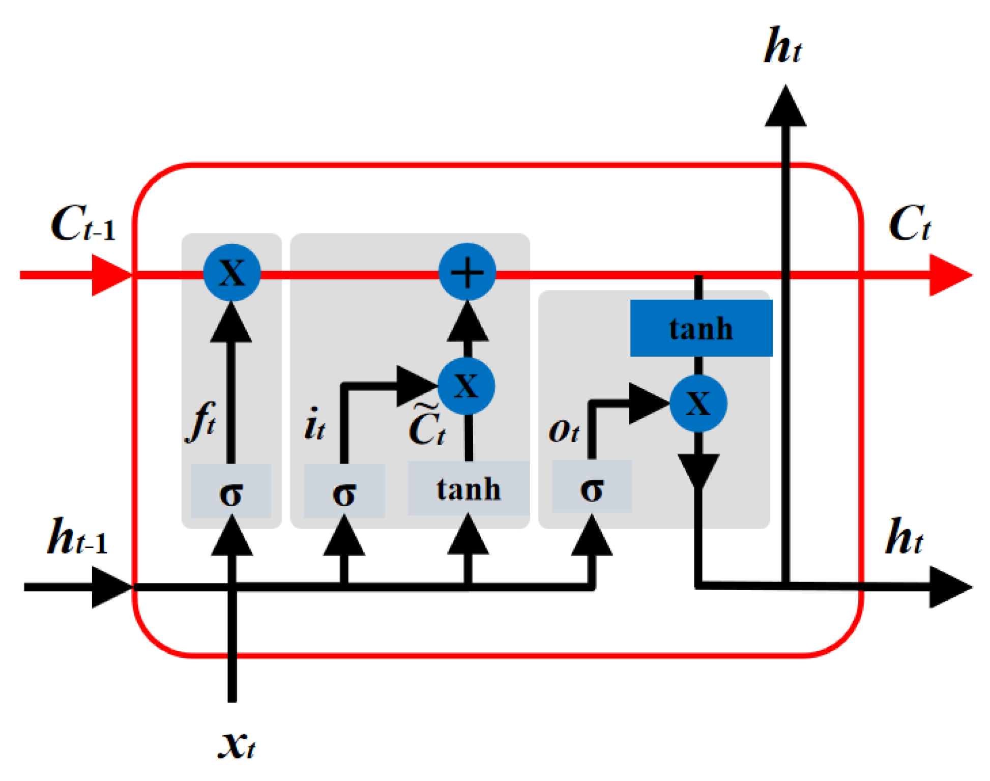
2.3.1. LSTM Unit

As a specialized recurrent neural network, the LSTM model excels in capturing the complex nonlinear and time-varying dynamics of time series. This capability stems from its gated architecture, which dynamically regulates information flow through learnable parameters to preserve long-term dependencies—crucial for modeling degradation trends in industrial systems. Each LSTM unit consists of a cell state and three primary components: the forget gate, the input gate, and the output gate. The detailed internal architecture is illustrated in Figure 2. The $x_t$ denotes the input data vector at time step t. The $h_{t-1}$ and $h_t$ represent the hidden states at the previous and the current time steps, respectively. Similarly, $C_{t-1}$ and $C_t$ correspond to the cell states at the previous and current time steps. The forget gate ($f_t$), input gate ($i_t$), candidate cell state (${\stackrel{\sim }{C}}_t$), and output gate ($o_t$) are the components represented here, with sigmoid function $\sigma (\cdot )$ and hyperbolic tangent function tanh(·) serving as the activation functions within the LSTM unit.

The forward propagation process is described by the following equations:

$$f_t=\sigma (W_f\ast \left[h_{t-1},x_t\right]+b_f),$$

(4)

$$i_t=\sigma (W_i\ast \left[h_{t-1},x_t\right]+b_i),$$

(5)

$${\stackrel{\sim }{C}}_t=\tanh (W_c\ast \left[h_{t-1},x_t\right]+b_c),$$

(6)

$$C_t=f_t\odot C_{t-1}+i_t\odot {\stackrel{\sim }{C}}_t,$$

(7)

$$o_t=\sigma (W_o\ast \left[h_{t-1},x_t\right]+b_o),$$

(8)

$$h_t=o_t\odot \tanh (C_t),$$

(9)

where W and b denote the corresponding weight matrices and bias vectors, respectively. During training, the backpropagation of errors occurs through each time step, enabling the calculation of gradients for all parameters. These gradients are then used to update and optimize the weights and bias terms. By performing both forward and backward propagation, the LSTM model effectively learns complex patterns and captures long-term dependencies present in time-series data.

2.3.2. Evaluation Metrics

Given the complexity and nonlinear characteristics of the multivariate wind turbine power estimation model, this study adopted a multi-metric evaluation strategy to provide a comprehensive and precise assessment of the model’s performance. In particular, four evaluation metrics were employed: MAE, RMSE, coefficient of determination (R²), and normalized mean absolute percentage error (NMAPE). Among these, a higher R² value indicates better model performance, whereas lower values are preferred for MAE, RMSE, and NMAPE. The formulas for these metrics are presented below:

$$\mathrm{MAE}={\displaystyle \frac{1}{N}}{\displaystyle \sum _{i=1}^N\left|{\stackrel{\wedge }{P}}_i-P_i\right|},$$

(10)

$$\mathrm{RMSE}=\sqrt{{\displaystyle \frac{1}{N}}{\displaystyle \sum _{i=1}^N{({\stackrel{\wedge }{P}}_i-P_i)}^2}},$$

(11)

$${\mathrm{R}}^2=1-{\displaystyle \frac{{\displaystyle \sum _{i=1}^N{({\stackrel{\wedge }{P}}_i-P_i)}^2}}{{\displaystyle \sum _{i=1}^N{(\overline{P}-P_i)}^2}}},$$

(12)

$$\mathrm{NMAPE}={\displaystyle \frac{1}{N}}{\displaystyle \sum _{i=1}^N\left|\frac{{\stackrel{\wedge }{P}}_i-P_i}{P_{\max }}\right|}\times 100\%,$$

(13)

where N is the number of samples, ${\stackrel{\wedge }{P}}_i$ and $P_i$ correspond to the estimated and actual values of the target variable, while $\overline{P}$ and $P_{\max }$ indicate the mean and maximum of the actual values.

2.4. Selection of Multivariable Environmental Factors

Wind turbine power generation is influenced by various environmental parameters, such as wind speed, wind direction, and air density. Selecting the environmental parameters that accurately represent the wind energy resources at the turbine location is a crucial step for achieving accurate modeling of multivariable power assessment. This selection is also fundamental for ensuring the accuracy of performance comparisons across different turbines. Based on aerodynamic principles, the mechanical power output of a wind turbine is determined by the following equation [19]:

$$P={\displaystyle \frac{1}{2}}{C}_p\rho A{V}_H^3,$$

(14)

where C_p denotes the wind energy utilization coefficient at the hub height wind speed, which is influenced by the tip speed ratio and the pitch angle, $\rho$ represents the air density, A stands for the rotor swept area, and V_H is the wind speed at the hub height.

The output power of a wind turbine is directly related to air density and the cube of the wind speed at the hub height, making these two environmental factors primary variables. Variations in wind direction over time also influence the turbine’s yaw performance; therefore, wind direction is typically represented by its cosine and sine components [25]. Wind speed exhibits considerable random fluctuations over time and displays notable spatial heterogeneity due to factors such as terrain, surface roughness, and atmospheric stability. Turbulence intensity is commonly employed to characterize the spatiotemporal variability of wind speed. Consequently, wind speed, air density, the cosine and sine of wind direction, and turbulence intensity were selected as input parameters for the multivariate power curve model. These parameters effectively capture the actual wind energy conditions at the turbine location and are relatively straightforward to obtain.

2.5. Power Assessment Model Framework

Based on the LSTM power assessment model illustrated in Figure 3, the following steps were undertaken: (1) abnormal state identification was performed through rigorous data cleaning, (2) time-series data samples were classified according to different control strategies, with the optimal time step length determined using the partial autocorrelation coefficient method, and (3) modeling was conducted using an LSTM architecture, with hyperparameter optimization carried out via grid search.

3. Results and Discussion

The dataset originated from the SCADA system of an offshore wind farm located in southern China and included data from three turbines, designated as units A, B, and C. These wind turbines are semi-direct drive, variable-speed, and variable-pitch units with a rated capacity of 5.5 MW. Detailed technical data of the wind turbines are listed in

Table 1. Detailed technical data of the wind turbine.

Parameters	Value	Units
Rated power	5.5	MW
Rotor diameter	155	m
Hub height	100	m
Cut-in wind speed	3	m/s
Rated wind speed	10.1	m/s
Cut-out wind speed	25	m/s
Blade tip speed	97.34	m/s
Gear transmission ratio	1:23.187
Blade pitch range	0 to 91	°

. Data were collected over the period from 1 January 2024 to 31 December 2024. Based on the criteria outlined in the previous section, the selected SCADA variables included wind speed, air density, the cosine and sine components of wind direction, turbulence intensity, and active power. Additionally, the operating mode measurement was incorporated to accurately identify each turbine’s operational state and to mitigate the influence of extended maintenance periods or fault conditions. All variables were aggregated as 10 min average values. The following will illustrate the model development process using turbine A as an example and, finally, compare the power generation performance of all three turbines under the same environmental conditions.

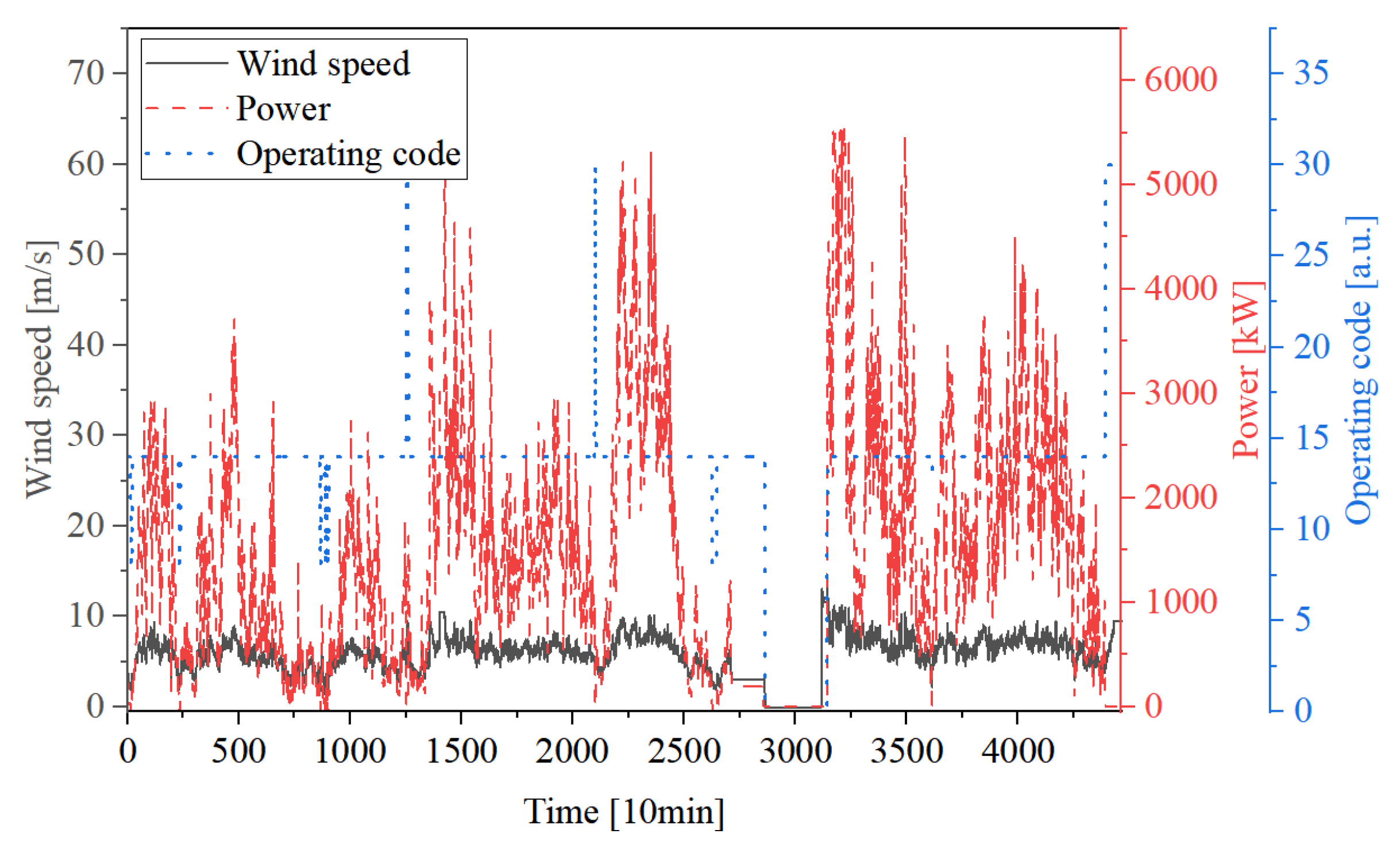
3.1. Wind Turbine Data Cleaning Results

The samples collected from the SCADA system were filtered based on the unit operation codes to exclude non-continuous power generation states. Figure 4 displays partial time series of feature variables for wind turbine A in January 2024. During operation, the wind turbine is in power generation mode when the code value equals 14. Code values from 1 to 10 represent different fault levels, while a code value of 30 indicates maintenance mode. As illustrated in Figure 4, the feature variables demonstrated notable volatility and included outliers during abnormal operating conditions. Consequently, to ensure the analysis reflected normal power generation, only data associated with code value 14 were utilized when constructing the model. The filtered data are shown in Figure 5. The points clustered at the bottom within the non-continuous power generation samples represent fault shutdowns or maintenance states, during which no power is generated. The outliers within the typical value range may be caused by start–stop state changes, fault operations, and other factors.

Subsequently, the power curtailment detection algorithm and the bidirectional quartile method were employed to identify abnormal samples. Data were binned into 0.5 m/s wind speed and 55 kW power intervals before applying the IQR. Figure 6a presents the anomaly detection results using only the bidirectional quartile method, whereas Figure 6b illustrates the results using a combination of the bidirectional quartile method and power curtailment detection. The combination approach achieved better filtering performance and successfully identified anomalies in the power curtailment transition region.

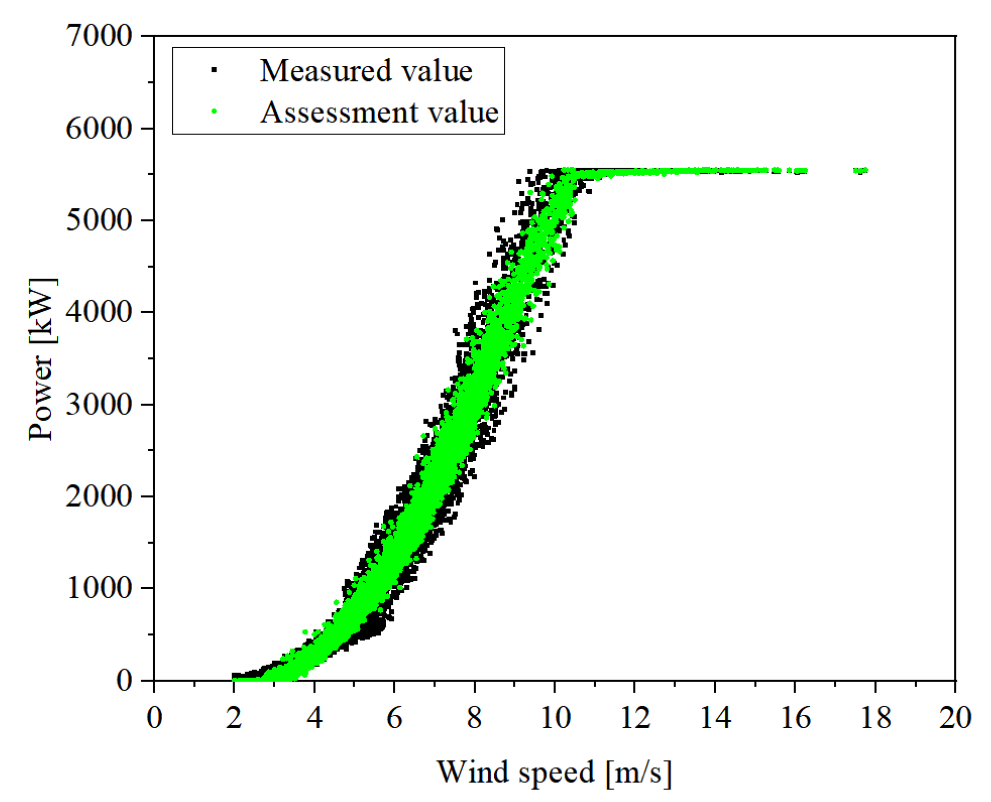
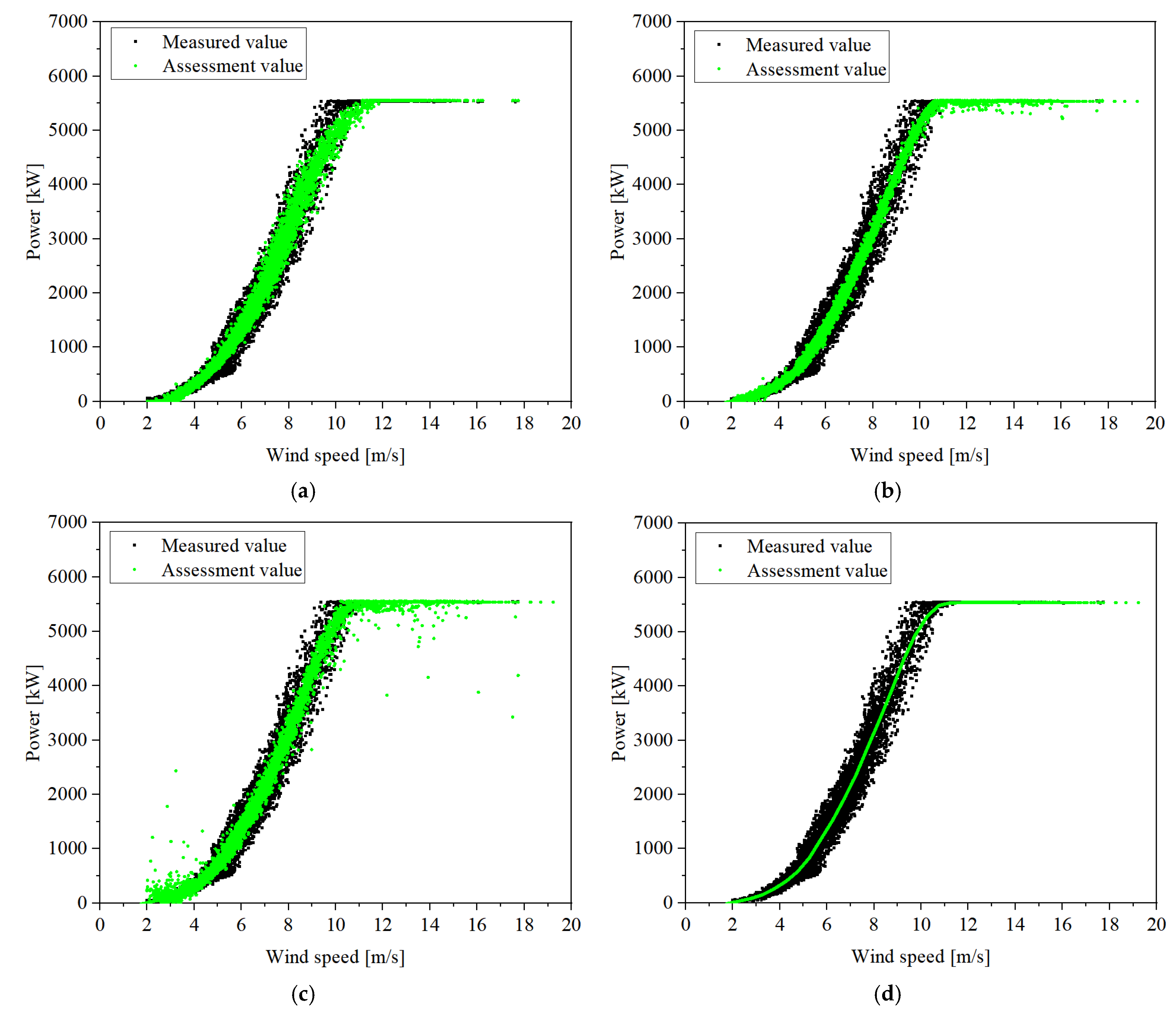
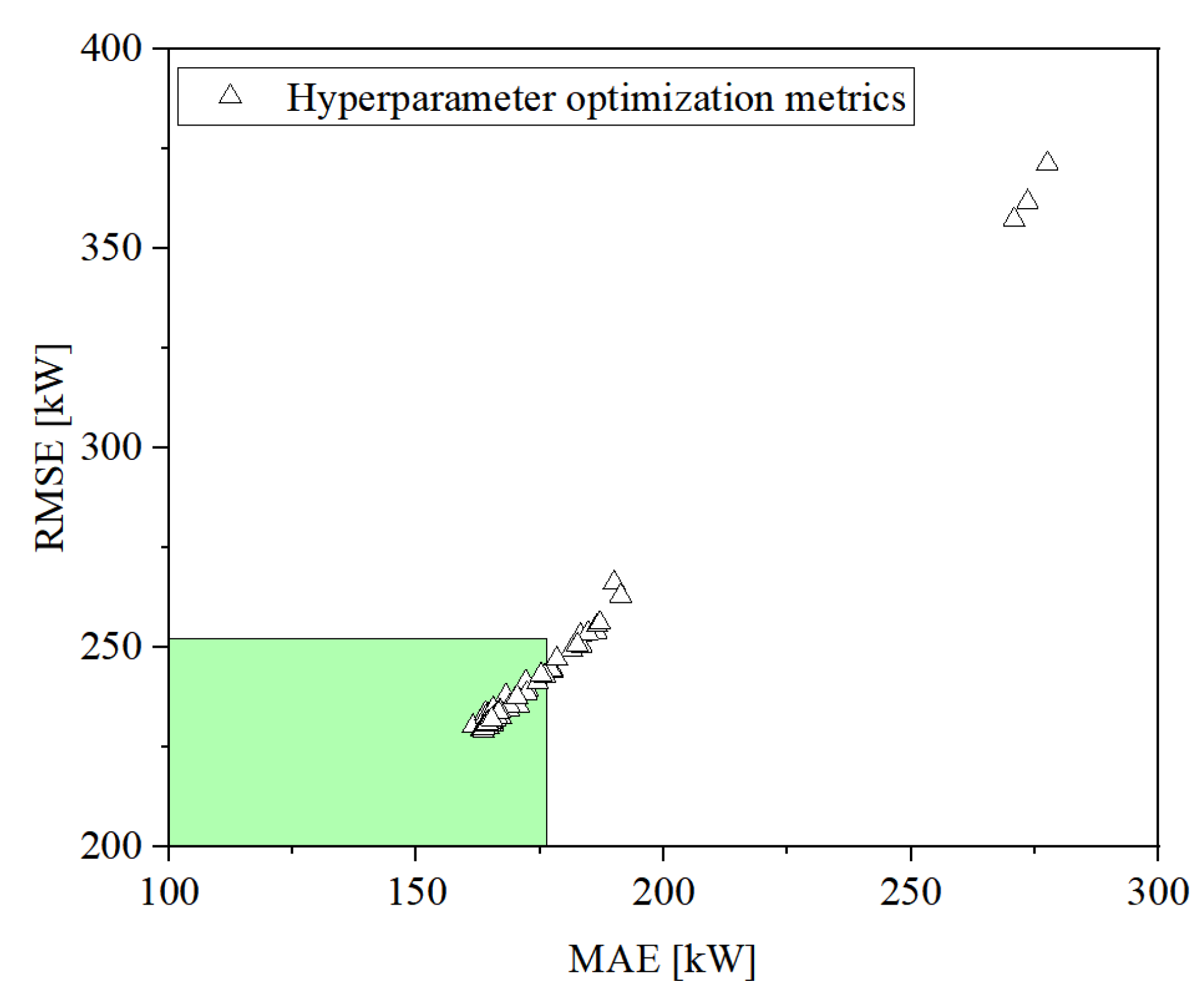
3.2. Proposed Model Training

The sliding window method was employed to construct data samples, allowing each window to capture both historical and current environmental parameters. The window width was determined by the lag corresponding to the maximum partial autocorrelation coefficient among all considered environmental variables. This study analyzed the partial autocorrelation coefficients of wind speed, air density, the cosine and sine components of wind direction, and turbulence intensity. Ultimately, a window size of 5 was chosen based on the maximum partial autocorrelation lag across all environmental variables. This choice was consistent with previous research [20] and ensured that the window effectively captured the most relevant temporal dependencies in the data.

Using the rated wind speed as the segmentation reference value, the samples were divided into two categories based on the final wind speed of each sample. Then, the data were split into training, validation, and test sets with a ratio of 6:2:2. During model training, min–max normalization was applied to both the input features and the target variables. Scaling the feature values to a consistent range helped to speed up the convergence of gradient descent algorithms. Hyperparameter tuning was conducted using a grid search across the following ranges: learning rate values of [0.1, 0.01, 0.001], hidden unit numbers of [16, 32, 64, 128, 256], and batch sizes of [32, 64, 128, 256, 512]. The power assessment results of the proposed model are shown in Figure 7. The assessment data obtained from the proposed model were highly consistent with the measured data.

To validate the improvement of the proposed model, it was compared with LSTM, BPNN, SVM, and the Bins method. The evaluation outcomes for various models are illustrated in Figure 8, with the corresponding metric values provided in

Table 2. Performance comparison of power assessment models.

Model	MAE (kW)	RMSE (kW)	R2	NMAPE (%)
Proposed	159.7231	222.3996	0.9793	2.8796
LSTM	161.4178	230.1190	0.9778	2.9101
BPNN	177.5985	251.0999	0.9736	3.2018
SVM	188.1254	266.4495	0.9703	3.3916
Bins method	176.2705	252.0215	0.9733	3.1758

. The proposed method demonstrated greater reliability by achieving the best overall performance across all evaluation metrics, with optimal values in MAE, RMSE, R², and NMAPE—consistently outperforming other models. This comprehensive superiority highlights its robust capability to minimize prediction uncertainty under complex operational scenarios. Based on the figures and tables, it can be seen that the performance of LSTM without segmentation ranked second, slightly inferior to the proposed method. As observed in Figure 8a, this model exhibited relatively large errors near the rated wind speed, which corresponded to the critical transition region between the MPPT region and the constant power region. This error concentration arose from two inherent limitations: (1) monolithic LSTM struggled to simultaneously learn contradictory control strategies (e.g., torque maximization vs. power limitation) across operational regions and (2) wind turbulence and pitch actuator dynamics near rated speed introduced high-frequency nonlinearities that exceeded the model’s generalization capacity without physical segmentation. In contrast, BPNN, SVM, and the Bins method performed relatively poorly, primarily due to their structural inability to exploit temporal dependencies in wind sequences. BPNN and SVM treat sequential data as independent points, discarding vital information that governs turbine dynamics, while the Bins method’s static averaging fails to capture transient control adjustments. These limitations manifest as systematic biases in regions with high volatility, as evidenced by their consistently higher MAE and RMSE in Table 2.

3.3. Performance Comparison of Wind Turbines

Following the aforementioned procedure, segmented LSTM models were developed separately for turbine B and turbine C. The cleaned multivariate environmental parameter data from turbine A were used as the input for all three turbines to obtain the cumulative power output, which was then applied to evaluate the performance degradation of the different wind turbines. The calculation results are presented in

Table 3. Total power generation of different wind turbines based on the environmental samples from wind turbine A.

Wind Turbine	Total Power Generation (MWh)	Max. Normalization
A	1029.0538	1.0000
B	881.3843	0.8565
C	943.7895	0.9171

. As shown in Table 3, under the same wind energy resource conditions, turbine A demonstrated better power performance compared to turbines B and C. The power generation of turbines B and C decreased by 14.35% and 8.29%, respectively, relative to turbine A. These results indicate that turbines B and C exhibited relatively poorer power performance and, therefore, should be prioritized for maintenance scheduling or technical retrofit plans in the upcoming maintenance cycle.

3.4. Discussion

This paper proposed performing outlier detection using a combination of the bidirectional quartile method and power curtailment detection after data preprocessing. As shown in Figure 6, this approach identifies power curtailment samples clustered within the typical value range, which is beneficial for the subsequent model development.

Meanwhile, samples were classified based on differences in wind turbine control strategies under varying wind speeds, followed by the establishment of LSTM models. Compared to the non-segmented LSTM, this approach achieved better performance. After hyperparameter optimization, the proposed model’s performance showed a reduction of 9.39% in MAE and 11.75% in RMSE relative to the traditional Bins method. The optimized non-segmented LSTM model also outperformed the Bins method. The LSTM performance metrics under different hyperparameters obtained through grid search are shown in Figure 9, where the green area represents regions outperforming the Bins method, highlighting the importance of hyperparameter optimization.

After separately establishing the proposed method models for different turbines, a unified input environment sample was used to compare their power generation performance. As shown in Table 3, wind turbine A demonstrated the best power generation performance, while wind turbine B performed the worst. Based on the SCADA operating codes, the total durations of power generation, fault, and maintenance states for the three turbines were calculated, as shown in Figure 10. Turbine B had the shortest total time in both power generation and fault states, but its maintenance time far exceeded that of turbines A and C, indicating the presence of high-level faults in turbine B. These faults may include issues such as gearbox malfunctions, generator overheating, or blade damage, all of which can significantly impact the turbine’s power generation performance. This was also reflected in the power generation performance measured by the proposed method. Meanwhile, turbines A and C had relatively similar total durations across the three states, making it difficult to determine the priority for the next round of scheduled maintenance. The proposed method revealed that the power generation of turbine C decreased by 8.29% compared to turbine A, providing a reference for establishing the maintenance priority order.

4. Conclusions

This paper proposed a segmented power assessment LSTM model based on multivariate environmental factors to compare the power generation performance of different wind turbines. An effective outlier detection method was developed by combining the bidirectional quartile method with power curtailment detection, covering various abnormal cases, including power curtailment samples within the typical value range. Considering changes in turbine control strategies, a segmented power assessment model was established, and its hyperparameters were optimized using grid search. Experimental results demonstrated that the proposed method reduced the MAE and RMSE by 9.39% and 11.75%, respectively, compared with the traditional Bins method. Using SCADA data from three turbines in a real offshore wind farm throughout 2024, a comparative analysis of power generation performance was conducted. Under similar environmental conditions, turbine A exhibited the best performance, while turbines B and C showed decreases in power generation of 14.35% and 8.29%, respectively, relative to turbine A. Further statistical analysis of operational status data revealed that turbine B experienced significantly longer maintenance durations than turbines A and C, suggesting the presence of higher-level faults that prolonged fault diagnosis and repair cycles. Future research will focus on continuously expanding the sample dataset and conducting in-depth analyses of the dynamic variations in wind turbine power generation performance over extended timescales, aiming to provide theoretical foundations and technical support for improving operational efficiency and reliability of wind turbines.

References

1. Wang, J.Z.; Wang, Y.; Jiang, P. The study and application of a novel hybrid forecasting model–A case study of wind speed forecasting in China. Appl. Energy 2015, 143, 472–488. [Google Scholar] [CrossRef]
2. Shao, H.; Henriques, R.; Morais, H.; Tedeschi, E. Power quality monitoring in electric grid integrating offshore wind energy: A review. Renew. Sustain. Energy Rev. 2024, 191, 114094. [Google Scholar] [CrossRef]
3. Guo, Y.; Wang, H.; Lian, J. Review of integrated installation technologies for offshore wind turbines: Current progress and future development trends. Energy Convers. Manag. 2022, 255, 115319. [Google Scholar] [CrossRef]
4. Kassa, B.Y.; Baheta, A.T.; Beyene, A. Current trends and innovations in enhancing the aerodynamic performance of small-scale, horizontal axis wind turbines: A review. ASME Open J. Eng. 2024, 3, 031001. [Google Scholar] [CrossRef]
5. Ghafoorian, F.; Wan, H.; Chegini, S. A systematic analysis of a small-scale HAWT configuration and aerodynamic performance optimization through kriging, factorial, and RSM methods. J. Appl. Comput. Mech. 2024, 11, 887–903. [Google Scholar]
6. Farajyar, S.; Ghafoorian, F.; Mehrpooya, M.; Asadbeigi, M. CFD investigation and optimization on the aerodynamic performance of a Savonius vertical axis wind turbine and its installation in a hybrid power supply system: A case study in Iran. Sustainability 2023, 15, 5318. [Google Scholar] [CrossRef]
7. Enevoldsen, P.; Valentine, S.V. Do onshore and offshore wind farm development patterns differ? Energy Sustain. Dev. 2016, 35, 41–51. [Google Scholar] [CrossRef]
8. Yan, J.; Zhang, H.; Liu, Y.; Han, S.; Li, L. Uncertainty estimation for wind energy conversion by probabilistic wind turbine power curve modelling. Appl. Energy 2019, 239, 1356–1370. [Google Scholar] [CrossRef]
9. Jung, C.; Schindler, D. A global wind farm potential index to increase energy yields and accessibility. Energy 2021, 231, 120923. [Google Scholar] [CrossRef]
10. Jung, C.; Schindler, D. Development of onshore wind turbine fleet counteracts climate change-induced reduction in global capacity factor. Nat. Energy 2022, 7, 608–619. [Google Scholar] [CrossRef]
11. Lee, G.; Ding, Y.; Genton, M.G.; Xie, L. Power curve estimation with multivariate environmental factors for inland and offshore wind farms. J. Am. Stat. Assoc. 2015, 110, 56–67. [Google Scholar] [CrossRef]
12. Cascianelli, S.; Astolfi, D.; Castellani, F.; Cucchiara, R.; Fravolini, M.L. Wind turbine power curve monitoring based on environmental and operational data. IEEE Trans. Ind. Inform. 2021, 18, 5209–5218. [Google Scholar] [CrossRef]
13. Janssens, O.; Noppe, N.; Devriendt, C.; de Walle, V.; Hoecke, V. Data-driven multivariate power curve modeling of offshore wind turbines. Eng. Appl. Artif. Intell. 2016, 55, 331–338. [Google Scholar] [CrossRef]
14. Saint-Drenan, Y.M.; Besseau, R.; Jansen, M.; Staffell, I.; Troccoli, A.; Dubus, L.; Schmidt, J.; Gruber, K.; Simões, S.G.; Heier, S. A parametric model for wind turbine power curves incorporating environmental conditions. Renew. Energy 2020, 157, 754–768. [Google Scholar] [CrossRef]
15. Astolfi, D.; Castellani, F.; Lombardi, A.; Terzi, L. Multivariate SCADA data analysis methods for real-world wind turbine power curve monitoring. Energies 2021, 14, 1105. [Google Scholar] [CrossRef]
16. Guo, P.; Infield, D. Wind turbine power curve modeling and monitoring with Gaussian process and SPRT. IEEE Trans. Sustain. Energy 2018, 11, 107–115. [Google Scholar] [CrossRef]
17. IEC 61400-12-1:2017; Wind energy generation systems – Part 12-1: Power performance measurements of electricity producing wind turbines. International Electrotechnical Commission: Geneva, Switzerland, 2017.
18. Mushtaq, K.; Zou, R.; Waris, A.; Yang, K.; Wang, J.; Iqbal, J.; Jameel, M. Multivariate wind power curve modeling using multivariate adaptive regression splines and regression trees. PLoS ONE 2023, 18, e0290316. [Google Scholar] [CrossRef] [PubMed]
19. Wang, B.; Zhou, B.; Zhu, D.; Zou, M.; Luo, H. Pre-Filtering SCADA data for enhanced machine learning-based multivariate power estimation in wind turbines. J. Mar. Sci. Eng. 2025, 13, 410. [Google Scholar] [CrossRef]
20. Qiao, Y.; Han, S.; Zhang, Y.; Liu, Y.; Yan, J. A multivariable wind turbine power curve modeling method considering segment control differences and short-time self-dependence. Renew. Energy 2024, 222, 119894. [Google Scholar] [CrossRef]
21. Bischl, B.; Binder, M.; Lang, M.; Pielok, T.; Richter, J.; Coors, S.; Thomas, J.; Ullmann, T.; Becker, M.; Boulesteix, A.L.; et al. Hyperparameter optimization: Foundations, algorithms, best practices, and open challenges. Wiley Interdiscip. Rev. Data Min. Knowl. Discov. 2023, 13, e1484. [Google Scholar] [CrossRef]
22. Pandit, R.K.; Infield, D. Comparative assessments of binned and support vector regression-based blade pitch curve of a wind turbine for the purpose of condition monitoring. Int. J. Energy Environ. Eng. 2019, 10, 181–188. [Google Scholar] [CrossRef]
23. Karamichailidou, D.; Kaloutsa, V.; Alexandridis, A. Wind turbine power curve modeling using radial basis function neural networks and tabu search. Renew. Energy 2021, 163, 2137–2152. [Google Scholar] [CrossRef]
24. Tao, T.; Liu, Y.; Qiao, Y.; Gao, L.; Lu, J.; Zhang, C.; Wang, Y. Wind turbine blade icing diagnosis using hybrid features and Stacked-XGBoost algorithm. Renew. Energy 2021, 180, 1004–1013. [Google Scholar] [CrossRef]
25. Meng, A.; Chen, S.; Ou, Z.; Ding, W.; Zhou, H.; Fan, J.; Yin, H. A hybrid deep learning architecture for wind power prediction based on bi-attention mechanism and crisscross optimization. Energy 2022, 238, 121795. [Google Scholar] [CrossRef]
Figure 1. Operating zones of a wind turbine with variable speed and pitch control.
Jmse 13 01377 g001
Figure 2. Schematic of the LSTM unit.
Jmse 13 01377 g002
Figure 3. Schematic of the LSTM power assessment model.
Jmse 13 01377 g003
Figure 4. Time-series plots of wind speed, power, and operating code for turbine A in January 2024.
Jmse 13 01377 g004
Figure 5. Filtered plots of wind speed and power samples for turbine A in 2024.
Jmse 13 01377 g005
Figure 6. Anomaly detection results using (a) the bidirectional quartile method only and (b) a combination of the bidirectional quartile method and power curtailment detection.
Jmse 13 01377 g006
Figure 7. The power assessment results of the proposed model.
Jmse 13 01377 g007
Figure 8. The power assessment results of the proposed model: (a) LSTM without segmentation, (b) BPNN, (c) SVM, and (d) the Bins method.
Jmse 13 01377 g008
Figure 9. Performance metrics of LSTM under different hyperparameters, where the green area represents regions outperforming the Bins method.
Jmse 13 01377 g009
Figure 10. Total time of power generation, fault, and maintenance states for the wind turbines in 2024.
Jmse 13 01377 g010