Article

Wake Characteristics and Thermal Properties of Underwater Vehicle Based on DDES Numerical Simulation

1
Naval Architecture and Ocean Engineering College, Dalian Maritime University, Dalian 116026, China
2
Wuhan Second Ship Design and Research Institute, Wuhan 430205, China
*
Authors to whom correspondence should be addressed.
J. Mar. Sci. Eng. 2025, 13(7), 1371; https://doi.org/10.3390/jmse13071371
Submission received: 25 June 2025 / Revised: 13 July 2025 / Accepted: 16 July 2025 / Published: 18 July 2025
(This article belongs to the Special Issue Advanced Studies in Ship Fluid Mechanics)

Abstract

Investigating the coupled hydrodynamic and thermal wakes induced by underwater vehicles is vital for non-acoustic detection and environmental monitoring. Here, the standard SUBOFF model is simulated under eight operating conditions—speeds of 10, 15, and 20 kn; depths of 10, 20, and 30 m; and both with and without thermal discharge—using Delayed Detached Eddy Simulation (DDES) coupled with the Volume of Fluid (VOF) method. Results indicate that, under heat emission conditions, higher speeds accelerate wake temperature decay, making the thermal wake difficult to detect downstream; without heat emission, turbulent mixing dominates the temperature field, and speed effects are minor. With increased speed, wake vorticity at a fixed location grows by about 30%, free-surface wave height rises from 0.05 to 0.15 m, and wavelength remains around 1.8 m, all positively correlated with speed. Dive depth is negatively correlated with wave height, decreasing from 0.15 to 0.04 m as depth increases from 5 to 20 m, while wavelength remains largely unchanged. At a 10 m submergence depth, the thermal wake is clearly detectable on the surface but becomes hard to detect beyond 20 m, indicating a pronounced depth effect on its visibility. These results not only confirm the positive correlation between vessel speed and wake vorticity reported in earlier studies but also extend those findings by providing the first quantitative evaluation of how submergence depth critically limits thermal wake visibility beyond 20 m. This research provides quantitative evaluations of wake characteristics under varying speeds, depths, and heat emissions, offering valuable insights for stealth navigation and detection technologies.

1. Introduction

With the rapid development of science and technology and the growing understanding of the oceans and seas, underwater space has become a new focus of international strategic competition. It is more and more important that we develop marine energy resources and safeguard maritime security. An underwater vehicle is a vehicle that navigates underwater by remote control or automatic control. It is widely used for ocean exploration, surveillance, reconnaissance, intelligence collection, communication, navigation, and payload transport in military and civil fields. Detecting underwater vehicles has been one of the important issues in the marine security field. Underwater vehicles play a critical role in naval operations, scientific exploration, and subsea resource development. A vehicle’s wake—the region of complex vortex structures and turbulent mixing trailing behind it—strongly influences its hydrodynamic performance, acoustic signature, and thermal footprint. Coherent vortical motions in the wake can enhance flow unsteadiness, increase drag, and generate pressure fluctuations that propagate into the far field, potentially betraying the vehicle’s position. Meanwhile, heat transfer between the hull and the surrounding water governs the thermal plume, which is a key factor in infrared detection and environmental impact. A detailed understanding of both wake dynamics and thermal behavior is therefore essential for optimizing design, reducing detectability, and ensuring mission safety.
So far, it is common that underwater vehicles are detected by way of underwater acoustic transmission methods. It is known to the public that underwater acoustic wave transmission has the characteristics of low relative loss and long transmission distance. A multi-beam fish finder fitted on fishing boats can effectively distinguish underwater vehicles, cables, steel burials, and underwater objects. However, through the application of vibration and noise reduction technology, the radiation noise of underwater vehicles is greatly reduced and the level of concealment is significantly improved. On the other hand, due to the complexity of the underwater acoustic environment, the performance of acoustic detection equipment is greatly affected by the environment. So, a lot of research is focusing on non-acoustic detecting methods, such as magnetic reconnaissance drones, which can carry out extensive investigations into relevant waters in channels [1]. The focus is on multi-dimensional perception. Developing multi-dimensional and diversified exploration methods is effective for solving the problem of complex acoustic underwater survey equipment and changeable underwater environments.
The ocean is a fluid which is layered in density, temperature, and salinity. Hydrodynamic disturbance of seawater caused by the action of propellers and crafts creates wake turbulence during ship and underwater vehicle navigation. The wake in the water, left for a long time, propagates in the vertical direction; therefore, it forms hydrodynamic wakes such as Bernoulli Hills and Kelvin Wakes on the sea surface. The hydrodynamic wake of an underwater vehicle can remain on the sea surface for more than 1 to 1.5 h and extend for more than 15 to 25 km [2]. The eddy flow around the vehicle and the wake eddy flow at the rear of the vehicle are formed by the water medium and the vehicle moving together when the wake propagates in the horizontal direction. The relative duration is longer, and the distance is longer. More vehicle track information is contained in the vehicle’s path, which can last for many days, and the characteristics change with time. The impact of the body movement and propeller rotation on the seawater and friction between a rigid body and a fluid generates some heat when the vehicle is sailing underwater. In comparison to the effect of friction on the temperature of seawater, the cooling water of the power plant discharged by the vehicle will cause the temperature of nearby water or even far-field water to increase significantly and plays a major role in the change in seawater temperature. Meanwhile, there are temperature differences and density differences between the steady flow field and cooling water. Due to heat exchange and the buoyancy effect, the warmer water in the wake will spread to the cooler water, and the heavy water below lifts warmer water to the surface, which forms a wake with obvious thermal characteristics. The real-time position of a submarine can be captured and tracked by detecting the thermal wake of the sea surface with a high-resolution infrared thermal imager. Under the influence of the volume effect and turbulent wake effect, there will be obvious wave phenomena on the surface when the submarine sails near the surface. Airborne radar and reconnaissance satellite detection can also track the approximate location of the submarine. Therefore, many domestic and foreign experts and scholars have carried out various studies on the non-acoustic characteristics of the wake.
Wu et al. [3,4] used a VOF multiphase flow model to numerically simulate a layered flow field. They studied the temperature uniformity and linear stratification of a two-dimensional flow field and captured the floating phenomenon of cooling water discharge at different times, in order to simplify the calculation of flow field, save calculation time and improve simulation efficiency. The changes in relevant parameters such as temperature and density of the wake field were analyzed in detail. In addition, the numerical simulation results regarding the influence of submarine depth and speed parameters on thermal wake were also obtained and compared with the experimental results of the Los Angeles shrinkage model of American submarines, so as to verify the numerical simulation method. Schetz JA et al. [5,6,7,8] studied the wake lift diffusion characteristics of elongated objects in the thermocline propelled by propellers. In 2014, Rudolf et al. [9] used a real-time Brillouin scattering liDAR system to measure water temperature profiles in a laboratory setting with an average accuracy of 0.07 degrees Celsius. Hong et al. [10] investigated the surface wake characteristics generated by a submarine moving underwater at a uniform temperature, using unsteady viscous numerical simulations based on the RANS equations and the VOF method, respectively. In 2024, Peng et al. [11] used a VOF-based multiphase flow model in Fluent to numerically simulate coolant discharge and thermal wake diffusion and buoyancy for a 10,000-ton submarine, revealing how wake diffusion varies with speed and depth and the formation of surface “cold spots.” In 2014, Chen et al. [12] conducted three-dimensional Navier–Stokes numerical simulations alongside laboratory IR experiments to study the “cold wake” temperature difference generated by a diesel-powered submarine in stratified seawater, demonstrating consistent cold wake signatures on the surface that agreed with the simulation and IR measurements. In 2017, Hu et al. [13] experimentally investigated the surface thermal characteristics of the thermal wake of a self-propelled remote-control submarine in a water channel, revealing that the wake consists of a hot area and a hot–cold mixed area and validating their findings with infrared imaging. Zhang et al. [14] employed a seawater infrared radiation model—accounting for surface emissivity, sky radiation, shadow occlusion, and atmospheric effects—to simulate the 8–14 μm infrared signatures of submarine thermal wakes and calculate detection ranges based on temperature differences, revealing how radiative characteristics vary with viewing angle, wind speed, wake temperature, and ambient temperature. Luo et al. [15] conducted numerical simulations—employing the RNG k-ε turbulence model and VOF method within a 3D unsteady incompressible RANS framework—to analyze the free-surface wake generated by a moving submerged body and its interaction with stochastic ocean waves. Existing studies have primarily focused on either hydrodynamic or thermal wakes and largely employed RANS simulations or experimental methods, failing to utilize high-fidelity numerical approaches to concurrently analyze the coupled effects of speed, depth, and heat emission on wake characteristics under identical model conditions.
This study develops a numerical simulation model to investigate the evolution of both submerged and surface wakes of an underwater vehicle in a flow field with uniform temperature and density. Balancing available computational resources and solution accuracy, the most efficient grid generation method was adopted. By introducing a delayed function into the Detached Eddy Simulation (DES) turbulence model, the Delayed Detached Eddy Simulation (DDES) approach was implemented. Using the established mesh and physical model supplemented with the energy conservation equation, we analyzed the effects of varying ship speed, diving depth, and heat release intensity on wake vorticity, surface wave behavior, and thermal diffusion. The results show that wake vorticity and surface wave characteristics are highly sensitive to vessel speed, whereas the thermal wake strongly depends on diving depth and heat emission rate. These findings provide theoretical and technical support for the non-acoustic detection of underwater vehicles and enrich the understanding of multiphysical wake phenomena in stratified ocean environments.

2. Numerical Theoretical Model

This chapter provides a concise overview of the CFD techniques employed in this study, primarily drawing on the theoretical research of Wang et al. [16,17], including the three conservation equations of fluid motion and related turbulence modeling methods.

2.1. Control Equation

The numerical simulation of fluid motion must satisfy three conservation laws that are the law of conservation of mass, the law of conservation of momentum, and the law of conservation of energy. The energy conversion caused by temperature change for the study of hydrodynamic characteristics of conventional surface ships and underwater bodies is ignored. The energy conservation equation is generally not considered. However, in this study, considering the thermal emissions of underwater vehicles, the governing equation is more complicated than conventional research. Therefore, it is necessary to add the energy equation to carry out research on this topic.

2.1.1. Equation of Continuity

The law of conservation of mass is generally represented by the continuity equation. The significance of this principle is that the increase in fluid mass within a differential volume over a unit of time is equal to the net mass flowing into that differential volume. The expression is shown in (1):
ρ t + ( ρ v ) = 0
In a rectangular coordinate system, the expression can be rewritten as
ρ t + ( ρ u ) x + ( ρ v ) y + ( ρ w ) z = 0
In the above expression, u , v , and w are the velocity components in three directions in a rectangular coordinate system, respectively. The value of the density of the steady flow does not change with time and is constant. Therefore, the first term on the left of expression (2) is 0. The density of an incompressible fluid is constant. Then, the continuity equation is as follows:
u x + v y + w z = 0

2.1.2. Momentum Conservation Equation

Formulas (4)–(6) are mathematical expressions of the law of conservation of momentum, which is called the Navier–Stokes equation, or the N-S equation.
ρ u t + ( ρ u U ) = p x + μ 2 u x 2 + 2 u y 2 + 2 u z 2 + F x
ρ v t + ( ρ v U ) = p y + μ 2 v x 2 + 2 v y 2 + 2 v z 2 + F y
ρ w t + ( ρ w U ) = p z + μ 2 w x 2 + 2 w y 2 + 2 w z 2 + F z
In this formula, F x , F y , and F z are the mass force components, p is the fluid pressure, and μ is the dynamic viscosity coefficient.

2.1.3. Energy Conservation Equation

The law of conservation of energy, or the first law of thermodynamics, can be understood as the increase in energy within a differential volume being equal to the net heat flowing into the volume and the work performed by external forces. Without considering the change in kinetic energy, the internal energy can be expressed by temperature T, and the energy equation is as follows:
( ρ T ) t + d i v ( ρ u T ) = d i v k c p g r a d T + S T
The expanded form of this expression is
( ρ T ) t + ( ρ u T ) x + ( ρ v T ) y + ( ρ w T ) z = x k c p T x + y k c p T y + z k c p T z + S T
In this formula, T is the temperature, k is the thermal conductivity, c p is the specific heat capacity, and S T is the energy source term.
The heat transfer process in a substance is called heat transfer [18], which is mainly divided into three basic ways: heat conduction, convection, and radiation. When there is a large temperature difference within a substance or between a variety of substances, the various methods of heat transfer will transfer heat from the high-temperature region to the low-temperature region. Heat transfer exists in the direct exchange of energy between molecules, and there is no macroscopic movement in the medium. Generally speaking, there is only one way of heat transfer in solids, and heat transfer in fluids is accompanied by heat convection. The heat transfer process of heat convection is the relative displacement of fluid particles, which only occurs in fluids. Natural convection and forced convection are two main forms of heat conduction accompanied by molecular motion. Natural convection is the difference in density caused by the temperature difference of the fluid. Forced convection is a flow process caused by external mechanical action. Increasing the flow rate of the fluid can accelerate the process of convective heat transfer. Thermal radiation is the electromagnetic radiation phenomenon that occurs when the object does not directly depend on the medium due to the temperature difference.

2.2. Turbulence Solving Method

Theoretically, N-S equations are closed. However, direct numerical simulation requires extremely high computing power and occupies huge computing resources, and it is difficult to be widely used in industrialization. Therefore, the Reynolds average method is used to decrease the average processing time for calculating the turbulent pulsation term. The RANS method simplifies the processing of time pulsation, thus reducing the calculation cost, and makes the numerical simulation widely used in practical engineering. However, this method introduces an additional nonlinear term, which leads to the non-closure of the N-S equation and thus produces a variety of turbulence models. The computational cost of the LES method is lower than that of DNS, but the computational resources required for most complex practical models are still relatively large. However, with the gradual improvement of computer computing performance, this method has begun to be widely used in industrial flow computing.
Although RANS accurately reproduces mean surface pressure distributions, it lacks the ability to resolve the transient, large-scale vortices that drive turbulent mixing and heat convection in a submarine’s wake. DDES, by resolving these eddies while modeling only the near-wall regions, provides the necessary unsteady flow resolution for reliable thermal wake predictions.
The separation vortex combines the advantages of RANS and LES. The RANS method is used in the area near the wall to reduce the grid and calculation, and the LES method is used in the area far from the wall to ensure that the large-scale separation flow can be captured. Only the mathematical expression of the model is given here:
t ( ρ k ) + x i ρ k u i = x j Γ k k x j + G k Y k + S k
t ( ρ ω ) + x i ρ ω u i = x i Γ ω ω x i + G ω Y ω + S ω
where Γ k and Γ ω , respectively, represent the effective diffusivity of k and ω . G k is the turbulent kinetic energy that is generated by the average velocity gradient. G ω represents the generation of special turbulent kinetic energy dissipation ω . k is turbulent kinetic energy. Y k and Y ω denote turbulence k and ω dissipation. Custom source entries for the user are S k and S ω . The concept is that by resolving all turbulence scales above a specified cutoff, one can capture the large-scale effects and quasi-ordered structures present in many unsteady, nonequilibrium processes—phenomena that RANS methods fail to represent—while avoiding the enormous computational cost of resolving all turbulence scales in direct numerical simulation. To prevent RANS regions from prematurely switching to LES mode, a delay function is introduced into the DDES formulation to adjust the turbulence length scale. Spalart [19] proposed the form of the delay function as follows:
f d = 1 tanh 8 r d 3
r d = v t + v u i j u i j κ 2 d 2
f d equals 0 in the boundary layer near the wall. f d equals 1 in a separate flow area away from the wall. Thus, the turbulence characteristic length scale in DDES is defined as
L D D E S = L R A N S f d m a x 0 , L R A N S L L E S
It can be seen that the redefined turbulent characteristic length scale LDDES ensures that the RANS model is used to calculate the boundary layer region near the wall.

3. Calculation Model and Numerical Verification

3.1. SUBOFF Computational Model

Figure 1 shows the two computational models used in this study. On the left is the SBUOFF AFF-8 submarine hull, derived from the SUBOFF standard model developed at the David Taylor Research Center and extensively validated in towing-tank tests. Its geometry comprises a 1.016 m forebody, a 2.229 m parallel midbody, and a 1.111 m afterbody, for a total length of 4.356 m and a maximum diameter of 0.508 m. The sail measures 0.368 m in length and 0.460 m in height, based on a 2:1 circular cross-section. Four NACA 0020 cruciform control surfaces, each with a tip chord of 0.152 m, are attached at the stern. On the right is a seven-blade, large-side oblique propeller with a diameter of 0.25 m. The blades are skewed at 45° to optimize tip vortex control. The mesh is refined in the blade-tip region to ensure a near-wall y + < 1 for accurate boundary-layer resolution.
In this study, the actual scale model is assumed to be a 1:20 amplified model. Therefore, speed and depth are defined by this standard. The parameters used in the simulation are obtained based on Froude number similarity conversion. Speed is defined in the following terms: 10 kn corresponds to 1.15 m/s, 15 kn corresponds to 1.75 m/s, and 20 kn corresponds to 2.30 m/s. The depth is defined as follows: 10 m corresponds to 0.5 m, 20 m corresponds to 1.0 m, and 30 m corresponds to 1.5 m. The depth is defined as the distance from the free water surface to the central axis of the submersible.

3.2. Calculation Domain and Grid Independence Verification

Based on the RANS method, the standard SUBOFF model and the seven-blade large-side oblique propeller are adopted. The calculation domain is set to be 60 m long, about 14 times the length range; 32 m wide, about 7 times the length range; and 12 m high, about 3 times the length range. The front end of the calculation domain is 10 m from the tail of the underwater vehicle, and the tail end of the calculation domain is 50 m from the tail of the underwater vehicle. The boundary conditions of the front end and both sides of the calculation domain are the velocity inlet, the tail end is the pressure outlet, and the bottom and top are walls.
The grid diagram used in this paper to calculate SUBOFF resistance is shown in Figure 2. The number of grids represents the accuracy of the calculation to some extent. Therefore, in order to eliminate the interference of the number of grids on the calculation results, this paper selects four sets of different numbers of grids for the grid division of the calculation domain. The numbers of Mesh1, Mesh2, Mesh3, and Mesh4 were 1.02 million, 1.53 million, 2.05 million, and 2.9 million. The encryption methods of different grids remain the same; only the size of the encryption grid is different.
Figure 3 shows the calculation results of SUBOFF resistance with different mesh sizes. As seen in the figure, as the number of grids increases, the resistance value gradually decreases, indicating that higher grid accuracy is achieved. However, considering the available computing resources, the third set of computational grids was chosen for this paper. This set offers a higher computational quality while also accounting for the actual computing resources. In the final mesh, we performed y+ monitoring on the submarine surface and propeller blades. For the submarine surface, the thickness of the first grid layer was designed to ensure that y+ < 1, with the actual instantaneous y+ values distributed between 0.2 and 0.9 (average approximately 0.5). For the propeller blades, further refinement was applied in the tip and leading-edge regions, targeting y+ < 2. The monitored y+ values ranged from 0.5 to 1.8 (average approximately 1.2). These y+ results indicate that our mesh can adequately resolve the boundary layer and is sufficient for DDESs.

3.3. Numerical Verification

Based on the published resistance test results of the SUBOFF model, in this paper, the speed point of 3.045 m/s for numerical resistance verification was selected, and comparing the calculated results with the test results, the error is only 1.2%. See Table 1.
In this paper, the surface pressure coefficient of the naked boat body without appendages was monitored, and the speed was 3.3439 m/s. The numerical calculation results were treated without dimensionality and compared with the experimental values of Huang et al. [20]. The pressure coefficient is defined as
C p = 2 ( p p 0 ) / ρ U 0 2
In this formula, p is pressure, p 0 is the pressure of the fluid (in the simulation, neither the free liquid surface nor the pressure gradient is considered; this item is 0), U 0 is the incoming flow velocity, and ρ is fluid density.
As can be seen from Figure 4, the numerical calculation results are consistent with the experimental data, indicating that the RANS method is a cost-effective method for submarine hydrodynamic research, which is not only fast in calculation speed but also high in accuracy.
In Figure 4, the surface pressure coefficient Cp of the bare hull without appendages shows differences at certain values of the independent variables. There are several main reasons for this difference: In experimental data, the pressure measurements are often taken at discrete points on the hull, and due to the limitations of experimental setups, the probe placement might not exactly correspond to the locations where the CFD simulations were conducted. Additionally, the experimental setup may introduce small perturbations that affect the pressure readings, especially near sharp geometric features like the bow. In the CFD simulation, the mesh resolution near the hull surface plays a crucial role. Although the grid is refined in the boundary layer, slight differences in mesh density and the treatment of boundary conditions (e.g., turbulence models and wall functions) could result in small variations in Cp, especially in regions with high pressure gradients. The areas where the discrepancies are observed (such as near x/L = 0) typically correspond to regions of high flow separation and vortex formation, where experimental uncertainty is generally higher due to the complex nature of the flow field. In CFD, flow separation is modeled numerically, which can slightly differ from the physical process in the experiment.

4. Underwater Vehicle Wake Characteristics and Wake Thermal Characteristics

In this paper, a virtual pool is used to simulate the self-propulsion of a fully attached SUBOFF with a homogeneous density flow field. The SUBOFF has two symmetrical cooling water discharge outlets, and the energy equation and VOF method are added to the numerical model. The influence of different speeds on the heat phenomena in the wake is studied. The different characteristics of thermal wake and wave generation in the water surface under different diving depths are studied.

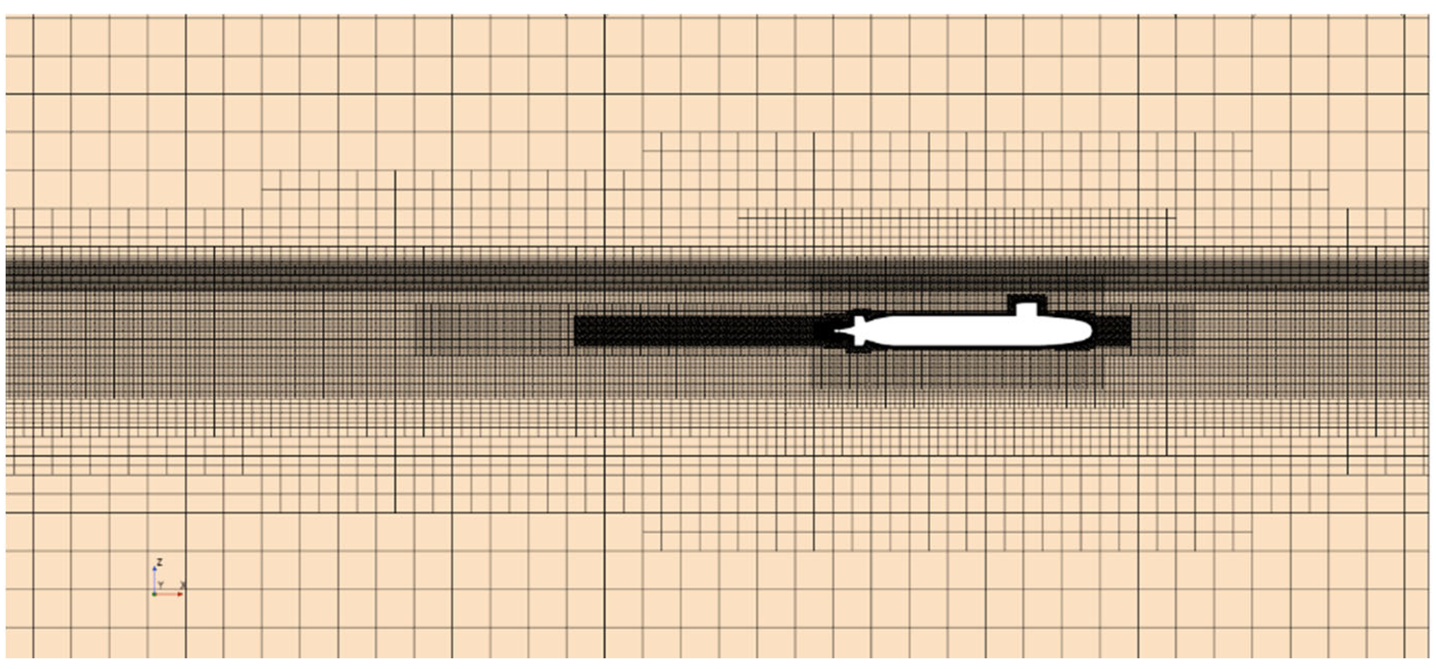
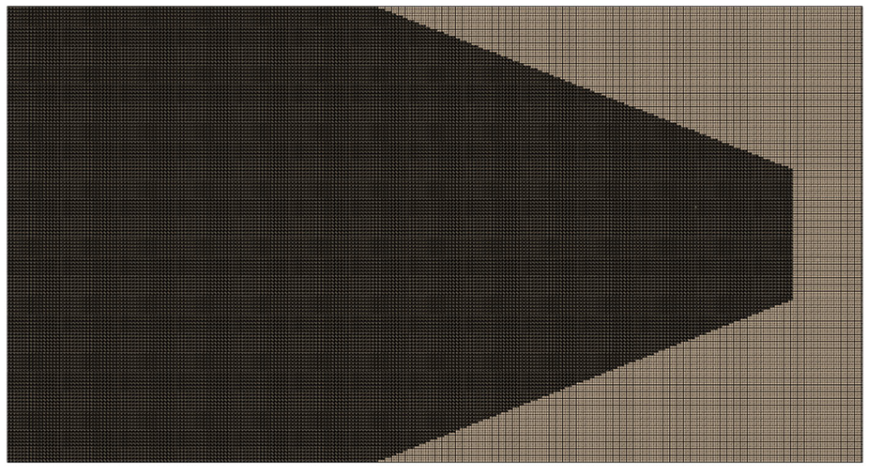
4.1. SUBOFF Model and Meshing

In the study of stratified flow fields with a free liquid surface and density, the geometric model in Figure 5 is adopted throughout the paper, so that the red circle in the lower figure is the heat discharge outlet.
In the SUBOFF standard model, two symmetrical cooling water discharge ports were added 0.04 m below the horizontal tail rudder, 0.34 m away from the tail end of the model in the horizontal direction, as shown in Figure 5, where the diameter of the cooling water discharge port was 0.02 m. Figure 6 and Figure 7 are the grids used in the simulation calculation in this paper, which are the longitudinal cross-section grid and the water surface grid, respectively. The content of this paper is slightly different from the mesh used in the numerical simulation in Section 2. First, the numerical simulation of the flow field under uniform density includes two-phase fluid of air and water, and there is a free liquid surface, and the mesh near the free liquid surface needs to be encrypted.
In order to make the water surface grid and the surrounding grid have a good transition, this paper encrypts the grid near the water surface with three layers, among which the most precise grid ensures at least 10 layers in the vertical direction and then gradually thins based on this grid. Since the wave generation of underwater vehicles is similar to that of surface ships, which generally presents a Kelvin wave Angle of 19°28′, in order to accurately encrypt the grid, improve the grid utilization rate, and reduce the total number of grids, this paper only encrypts the X and Y direction grids within the range of 19°28′. Secondly, the underwater vehicle will discharge cooling water. In order to accurately capture the thermal characteristics in the wake, it is necessary to encrypt the grid in the tail side of the underwater vehicle within a certain horizontal range, and the grid transition is also three-layered. The final number of grids will be adjusted with different working conditions, and the total number is generally about 8.6 million. The DDESs employed a mesh of approximately 8.6 million cells and were executed in parallel on 96 CPU cores. A representative case—advancing 30 s of physical time with a time step of 1 × 10⁻³ s—required about 18 h and peaked at around 70 GB of RAM. These figures serve as a practical benchmark for researchers planning similar DDES-based wake–thermal studies.

4.2. Numerical Model and Calculation Condition

In this paper, the delayed separation vortex (DDES) turbulence solution method is used for numerical simulation, and the free liquid surface is captured by the VOF method. All physical property parameters of air are fixed values. Under a flow field of uniform density, eight calculation conditions are formulated in this paper according to three parameters, speed, depth, and heat emission, as shown in Table 2:

4.3. Results and Analysis

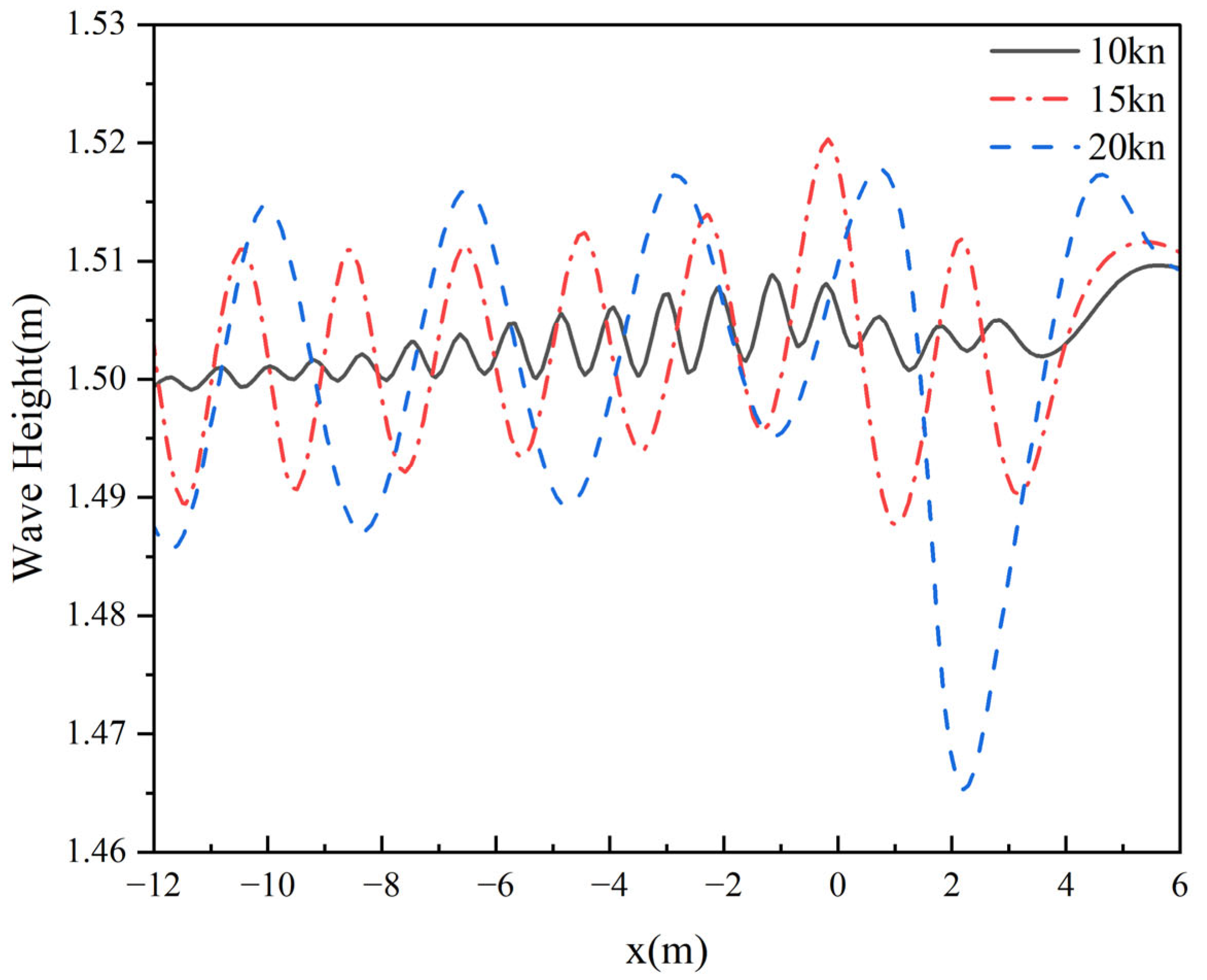
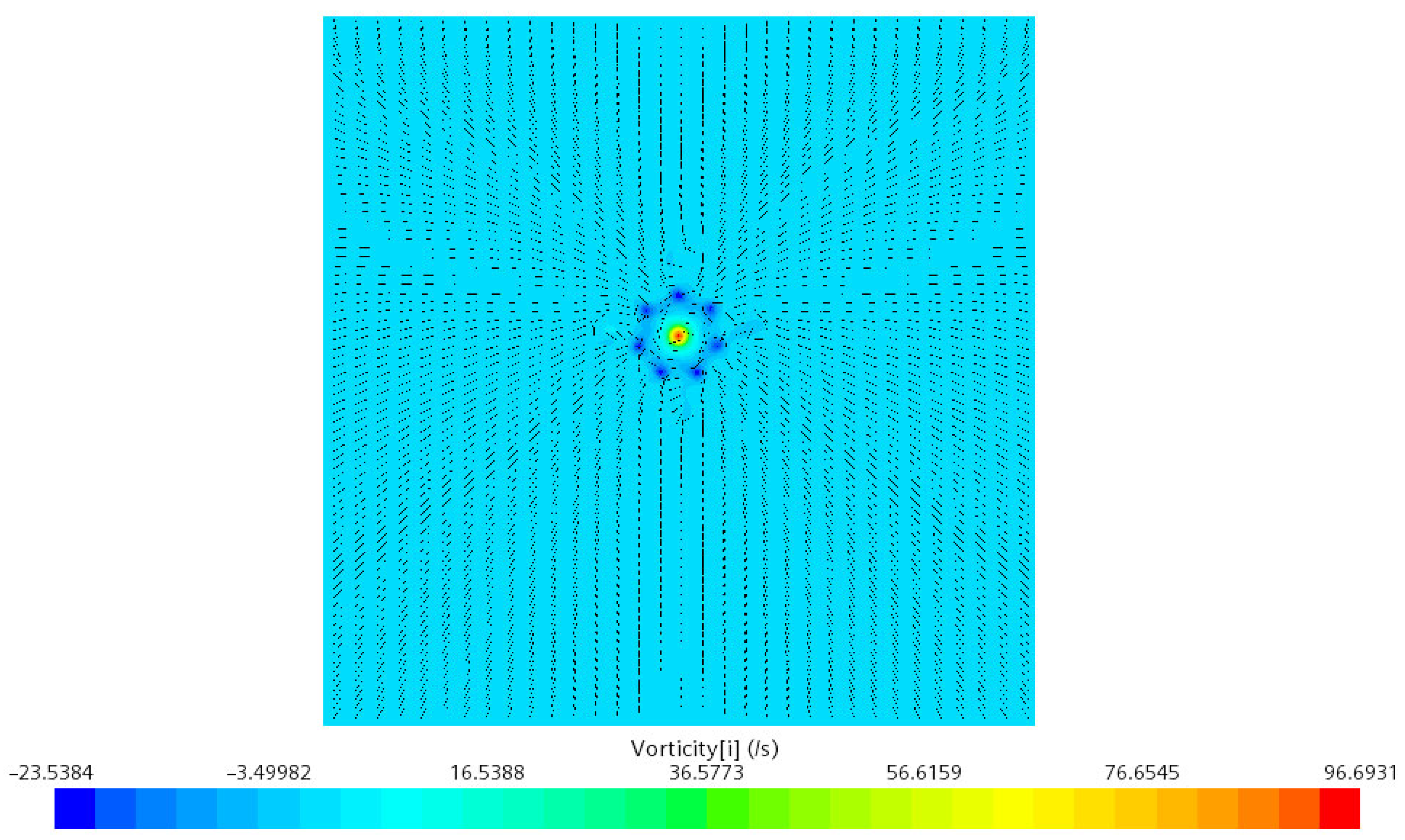
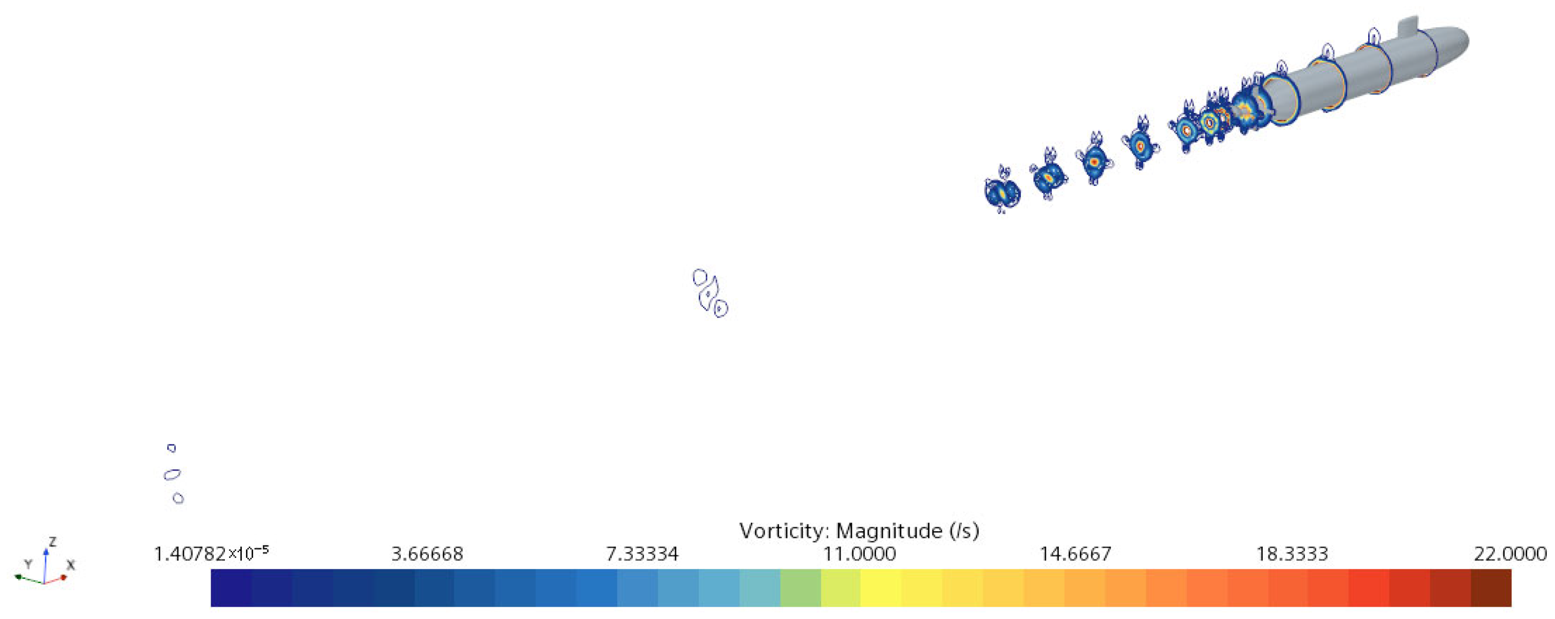
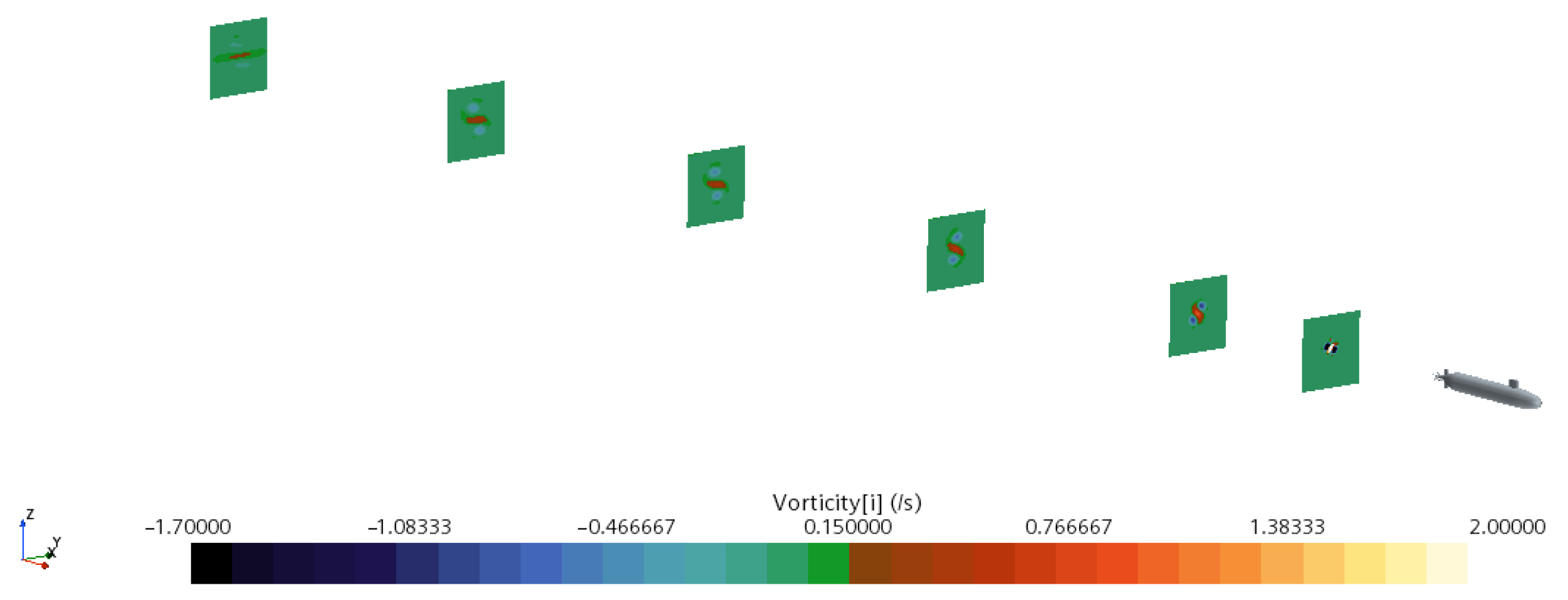
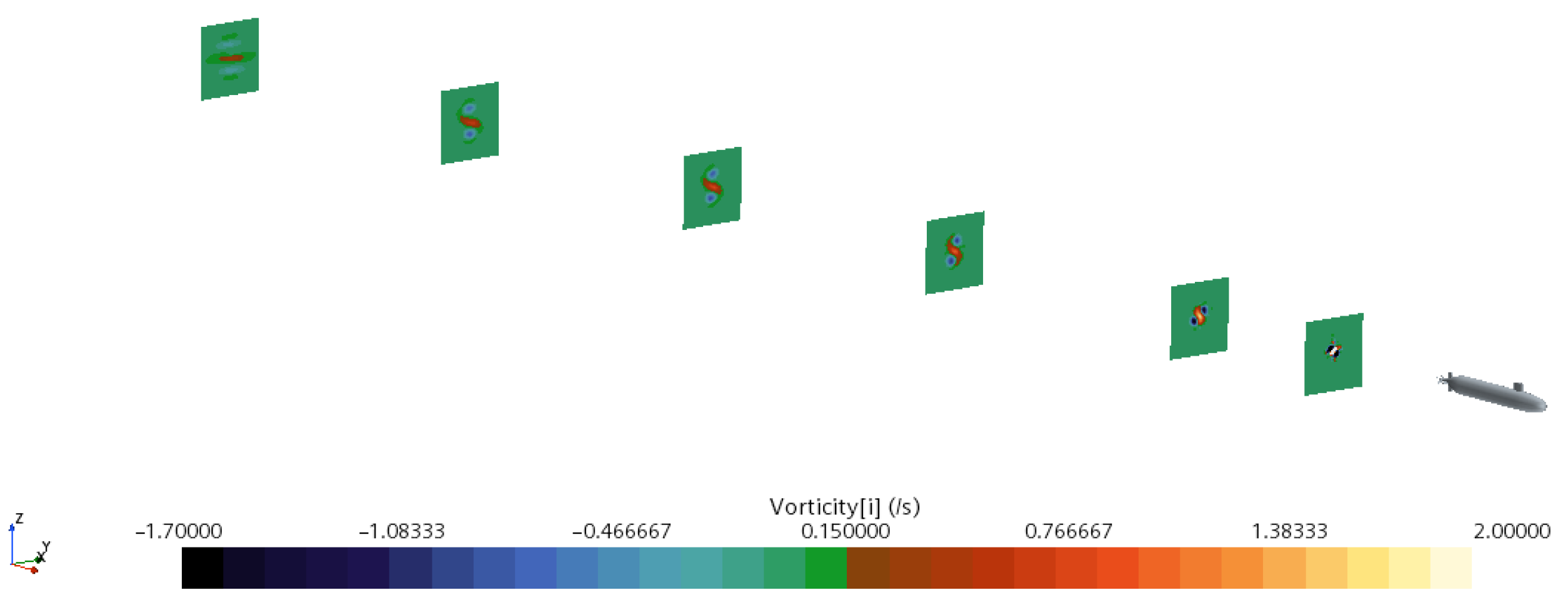
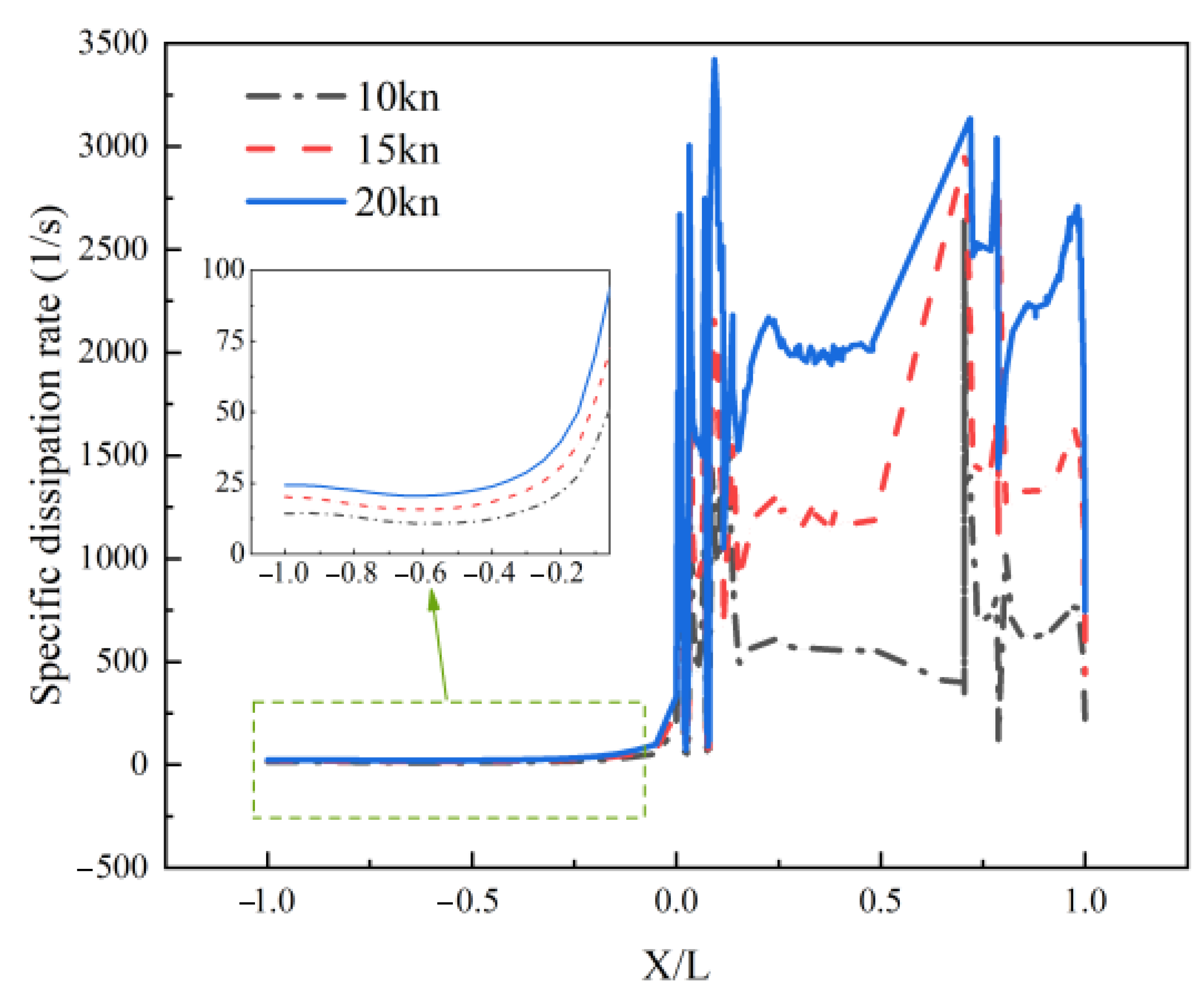
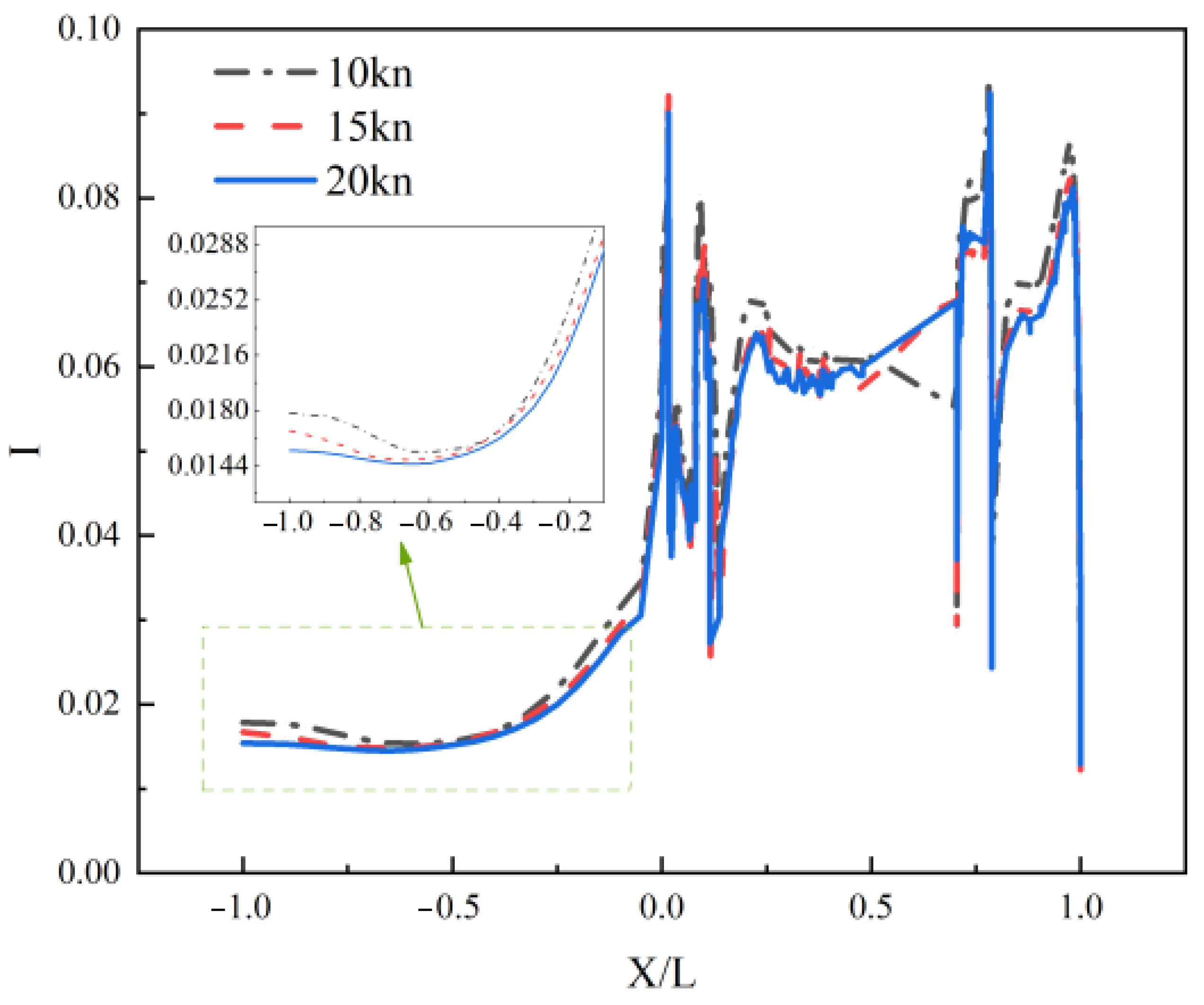
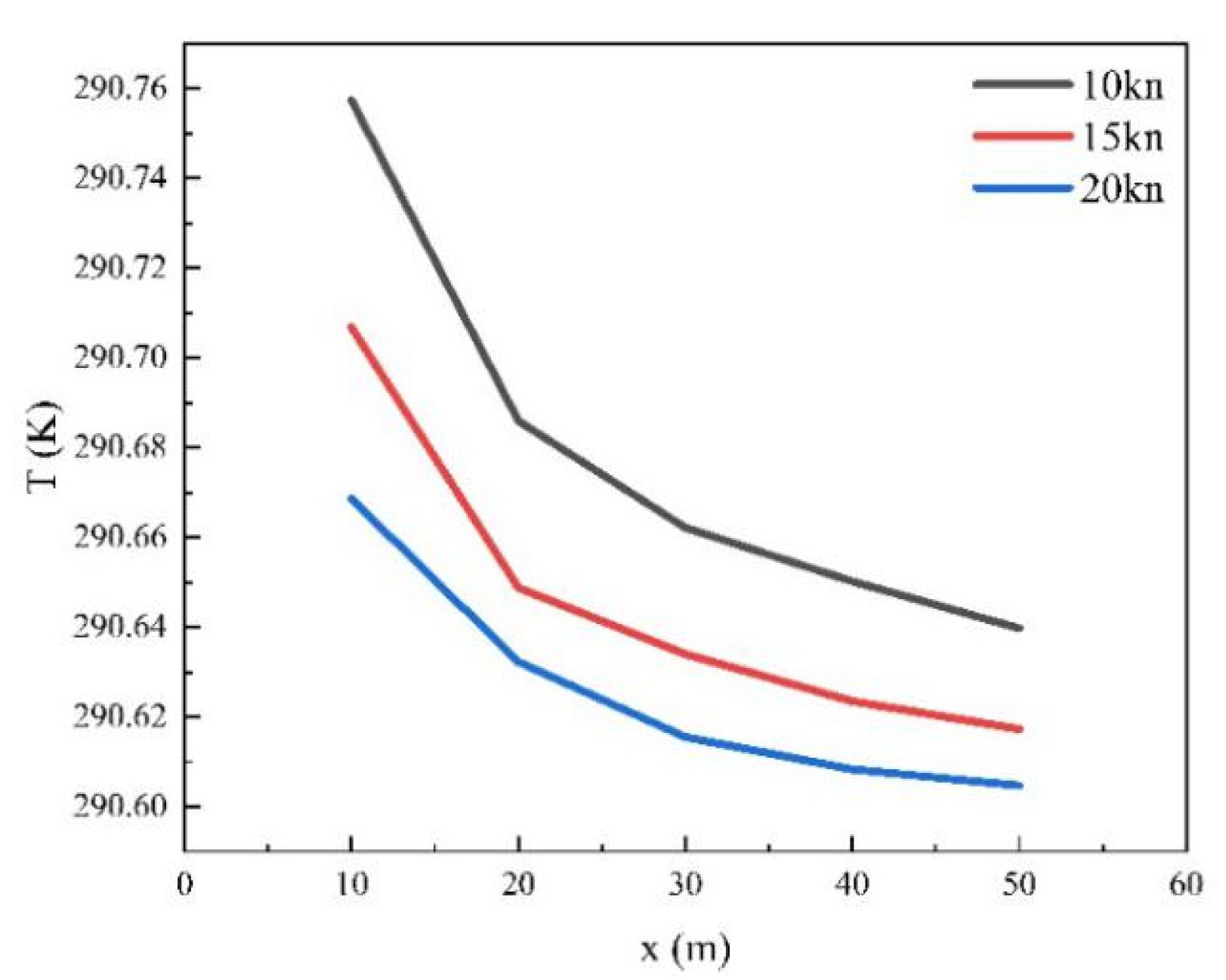
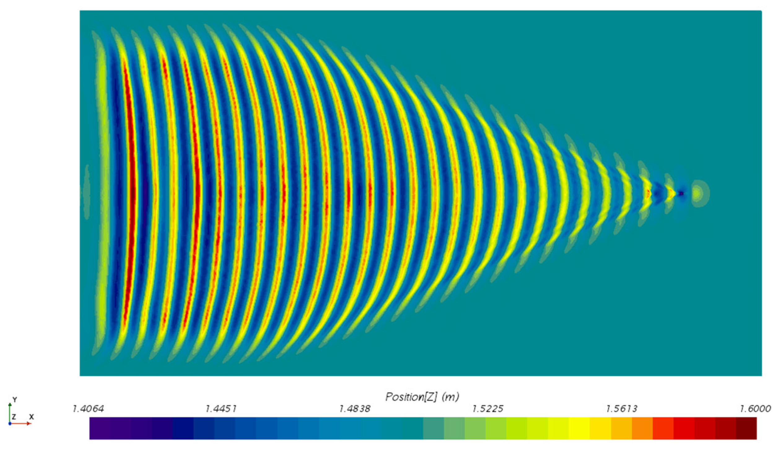
4.3.1. Influence of Speed on Hydrodynamic Wake Characteristics

The numerical calculations were performed for the operating conditions in Table 2 where speed is the variable, namely conditions 1, 4, and 7. In these conditions, the submarine’s diving depth is fixed at 20 m, and the submarine undergoes thermal emission with the same parameters (speed of 0.74 m/s and a temperature difference of 60 K). The wave generation on the water surface under each condition is shown in Figure 8, Figure 9 and Figure 10.
By analyzing the surface wave generation plots in Figure 8, Figure 9 and Figure 10, we observe that at a speed of 10 knots, the wake exhibits initial flow disturbances around the submarine. The wave structures are relatively weak, with moderate intensity in the far wake. The vortex patterns behind the hull are less pronounced compared to higher speeds, indicating lower energy in the wake flow. At 15 knots, the wake disturbances intensify, with clearer wave structures forming behind the submarine. The vortices become stronger, and the wake shows larger amplitudes compared to the 10-knot case. This indicates higher energy release into the water at this speed. At 20 knots, the wake becomes significantly more turbulent, with pronounced vortex formations and stronger wave activity in the far-field wake. The wake pattern is highly energetic, with large amplitude fluctuations in the water, reflecting the increased energy and fluid displacement caused by the higher speed and temperature differential. The primary difference between these figures lies in the intensity and extent of the wave and vortex patterns, which become more pronounced and stronger as speed increases. These variations reflect changes in the submarine’s hydrodynamic behavior as speed increases, accompanied by enhanced wake turbulence and energy dissipation.
Figure 11 shows the comparison of the wave height of the water surface at 19°28′ Kelvin, as well as the wave angle at different speeds. Through comparison, it was found that there is a positive correlation between the wave height of the water surface and ship speed within this range. The larger the ship speed is, the higher the wave height of the water surface is, and the more obvious the water wave is. In addition, observing the first three figures, it can be seen that the obvious reason for wave formation on the water surface is also related to the wavelength. The higher the speed, the longer the wavelength of wave formation on the water surface.
In order to further improve the credibility of the numerical simulation results in this paper, we sorted out the relationship between the wavelength of the water surface waves and the speed at three speeds, and we compared it with the results calculated by the empirical formula, which is Formula (15). Table 3 is plotted based on the calculation and simulation results as follows.
λ t h e o r y = 2 π U 2 g
In this formula, U is the speed, and λ is the wavelength.
The simulation results are basically consistent with those calculated by the empirical theoretical formula, and the error is very small, which further improves the reliability of the numerical simulation results in this paper.
The propulsion device used in this paper is a seven-blade large-side oblique propeller, so in the underwater wake, the vorticity diagram with the characteristics of propeller rotation will be presented. Figure 12 shows the section vorticity diagram extracted by axial vorticity and section velocity when the speed is 15 kn, where the section position X = −0.05 L.
When seawater flows through the vicinity of the propeller, the high-speed rotation of the propeller will change its motion mode, and flow separation will occur in the fluid, forming a center hub vortex and a surrounding tip vortex. The hub vortex is related to the hub of the propeller, and the tip vortex is related to the blade. There are seven blade blades in total, so seven corresponding tip vortices will be formed. And the shape of the vortex will also change to a certain extent, and it will eventually gradually maintain a steady flow field. In order to fully display the vortex structure behind the propeller, the Q criterion was adopted in this paper to extract the vortex diagram in the flow field, present the vortex structure in a three-dimensional manner, and color the vortex structure with a temperature field, as shown in Figure 13.
The meaning of the Q criterion is the possibility of vortices in the flow field. When Q is greater than 0, vortices may exist in the flow field. In this paper, the value of Q is set at 300. In this case, the vortex structure in the wake field can be clearly expressed, in which the outer ring is tip vortex and the inner ring is hub vortex, and this spiral vortex structure will gradually spread with the development of the wake. Its structure will become more and more blurred, and after a certain distance, it will completely dissipate in the background flow field.
Figure 13 also shows the mixing of cooling water and the spiral vortex. The thermal wastewater discharged by the underwater vehicle (red area) develops in the direction of an oblique upper angle through the rotation of the propeller, and it gradually diffuses into the whole tip vortex with the wake of the propeller, but it has little influence on the hub vortex.
Due to the rapid rotation speed of the propeller, the vorticity intensity in the wake is very strong, which will cover up the fluid flow separation caused by the characteristics of the main structure. In the figure, the real eddy current structure will be different from the eddy current structure shown, as the tiny structure cannot be reflected in the figure. In order to show the detailed eddy current structure, cross-sections near multiple subjects are selected to capture this feature in this paper.
Figure 14 shows the vortex diagram of the section near the main body. The maximum value of the color bar is fixed to 22, which can fully show the vortex structure differently from that in Figure 12. The main body of the fully attached SUBOFF model has a bridge and four tail rudders. When seawater flows through these special structures, a corresponding flow separation phenomenon will also occur. Therefore, in the vortex diagram, there will be a very obvious convex structure in front of the tail rudders, which is caused by the fluid flow separation near the bridge. There are also four distinct protruding structures around it, which are caused by fluid flow separation near the stern rudder, and the stern rudder directly above is in the same vertical plane as the bridge, so the flow separation phenomenon above is more obvious.
Figure 15, Figure 16 and Figure 17 show the vortexes of sections at different flight speeds, where the section distances from near to far are X = −4 m, −10 m, −20 m, −30 m, −40 m, and −50 m in order to unify the contrast effect. An analysis of the cross-sectional vortex distribution in submarine wakes at three different speeds (10 kn, 15 kn, 20 kn) reveals significant speed-dependent effects on vortex structures. At the nearest cross-section (X = −4 m), all three cases show concentrated high-intensity vorticity, with the 20 kn case exhibiting substantially greater extreme values compared to 10 kn and 15 kn, indicating that higher speeds intensify vortex separation near the hull. As the cross-sections move away from the submarine (from X = −10 m to −50 m), vorticity strength gradually diminishes in all cases, though the decay rate is noticeably slower at higher speeds (15 kn and 20 kn), where stronger vorticity characteristics persist even in far-field regions. In contrast, the 10 kn case shows near-zero vorticity at X = −50 m, demonstrating that high-speed vortex structures maintain greater far-field persistence. Additionally, while vorticity distribution remains relatively symmetrical at a low speed (10 kn), higher speeds lead to expanded positive vorticity regions with lateral displacement, likely due to enhanced flow asymmetry. The consistent color scale (−1.7~2.0) across all plots clearly demonstrates the positive correlation between speed and vorticity intensity, with the 20 kn near-field cross-section showing more pronounced color contrast and extreme values approaching the scale limits. These observations collectively highlight how increased speed significantly alters the spatial evolution of wake vorticity, providing valuable insights for optimizing submarine hydrodynamic performance.
The specific dissipation rate and turbulence intensity of the flow field extracted at 1 m behind the central axis and at the transversal surface of the underwater vehicle are shown in Figure 18 and Figure 19. When the submersible depth is 20 m, the specific dissipation rate at three speeds is shown in Figure 18, and the data within 1 m range of the underwater vehicle are locally amplified. The trend of the three curves is the same, in which there is a large range of fluctuations in the control tower enclosure and the tail rudder, and the specific dissipation rate increases with the increase in speed. When the submersible depth is 20 m, turbulence intensity at three speeds is shown in Figure 19. The turbulence intensity curve fluctuates in a large range at the control platform envelope and the tail rudder. However, the three curves have little difference and basically coincide. The speed has little influence on the turbulence intensity at the same depth.

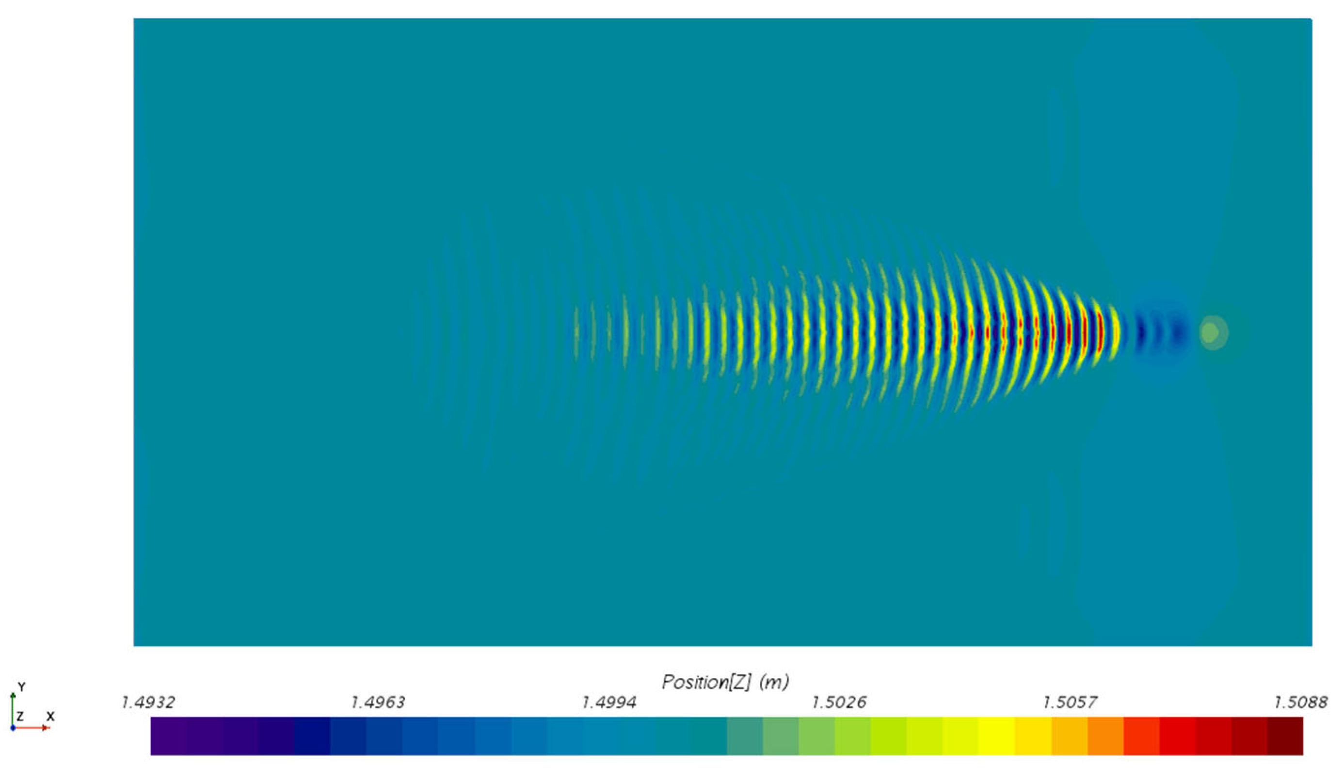
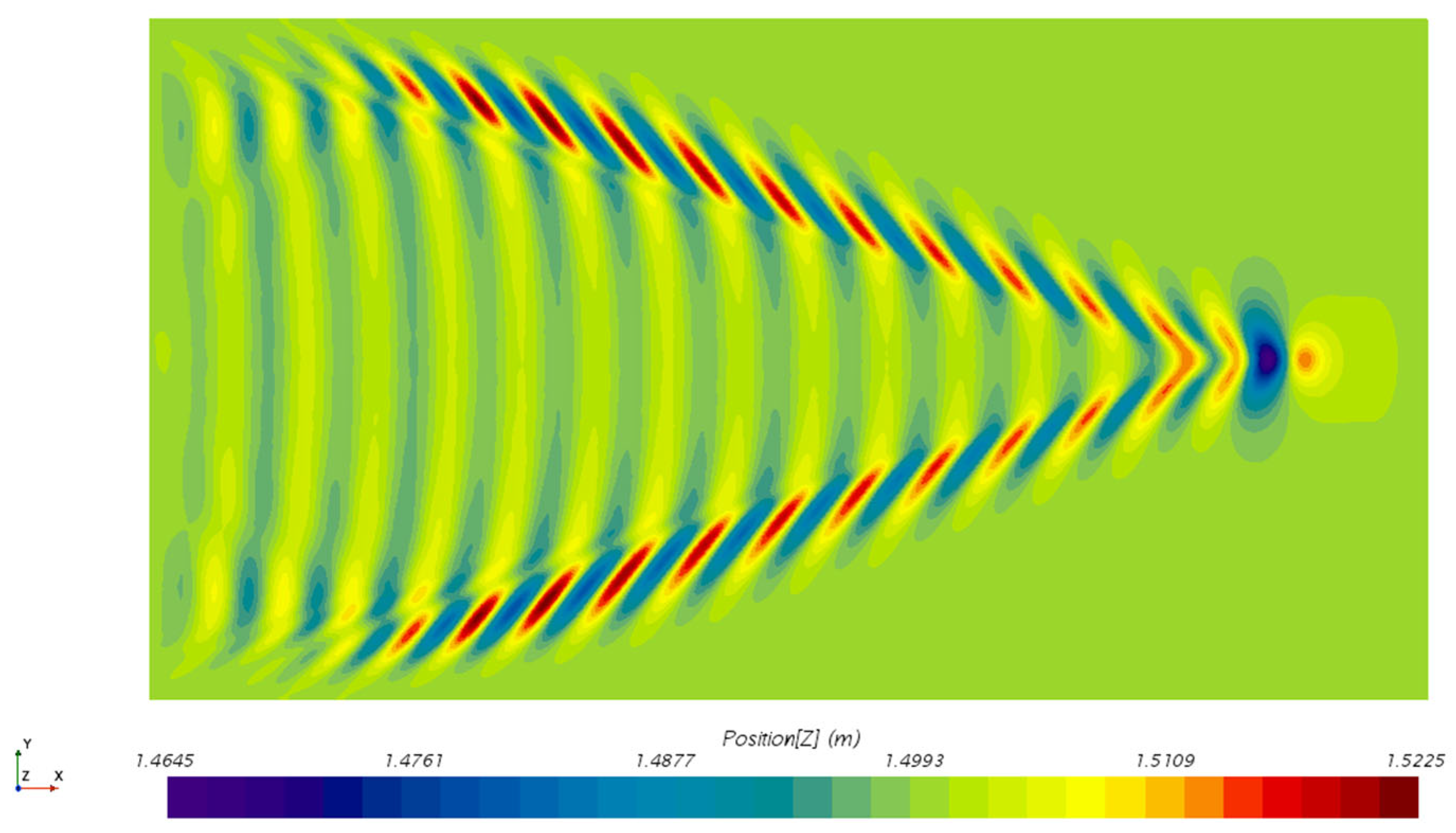
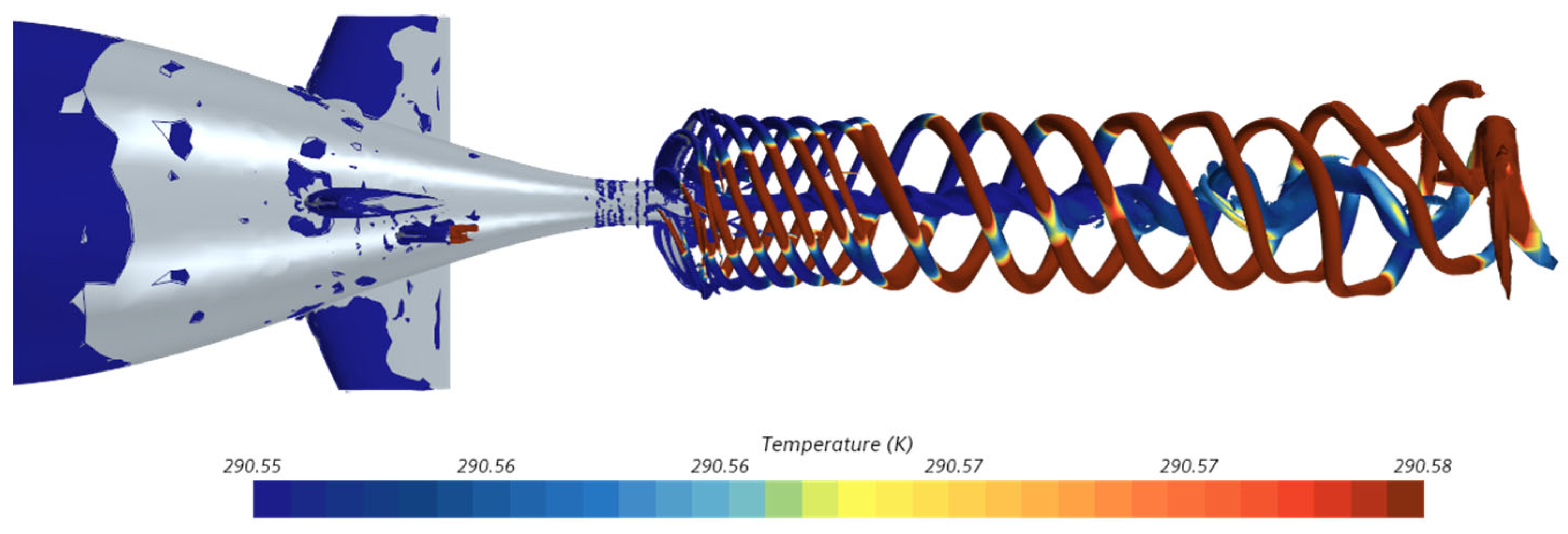
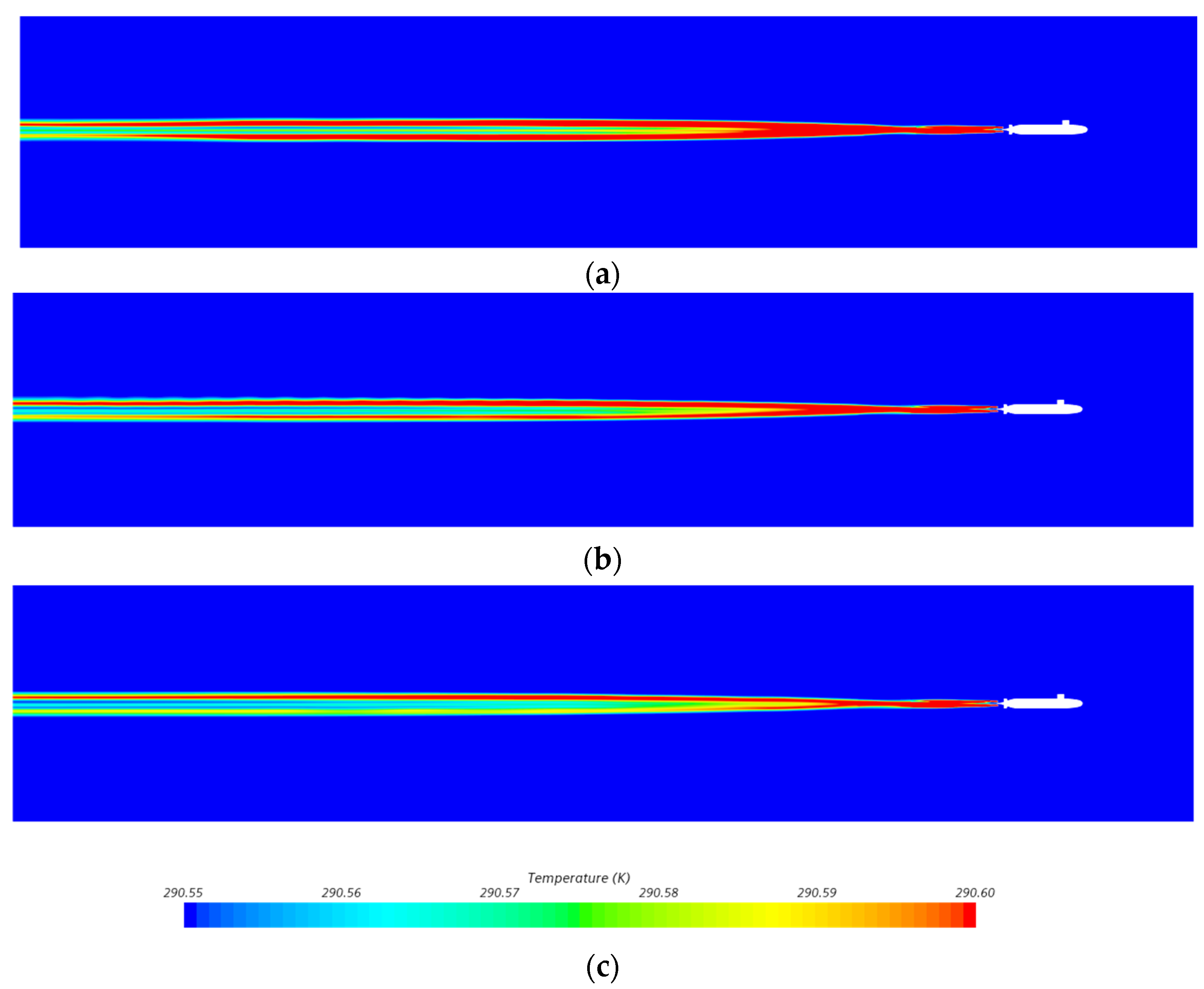
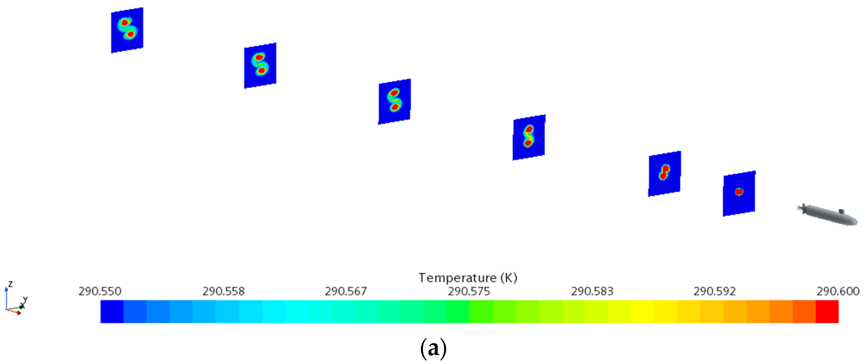
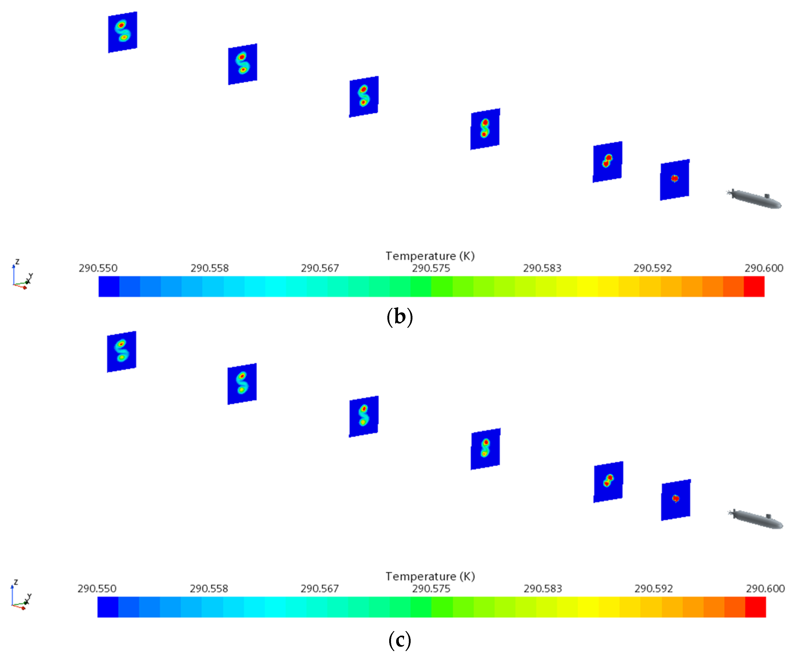
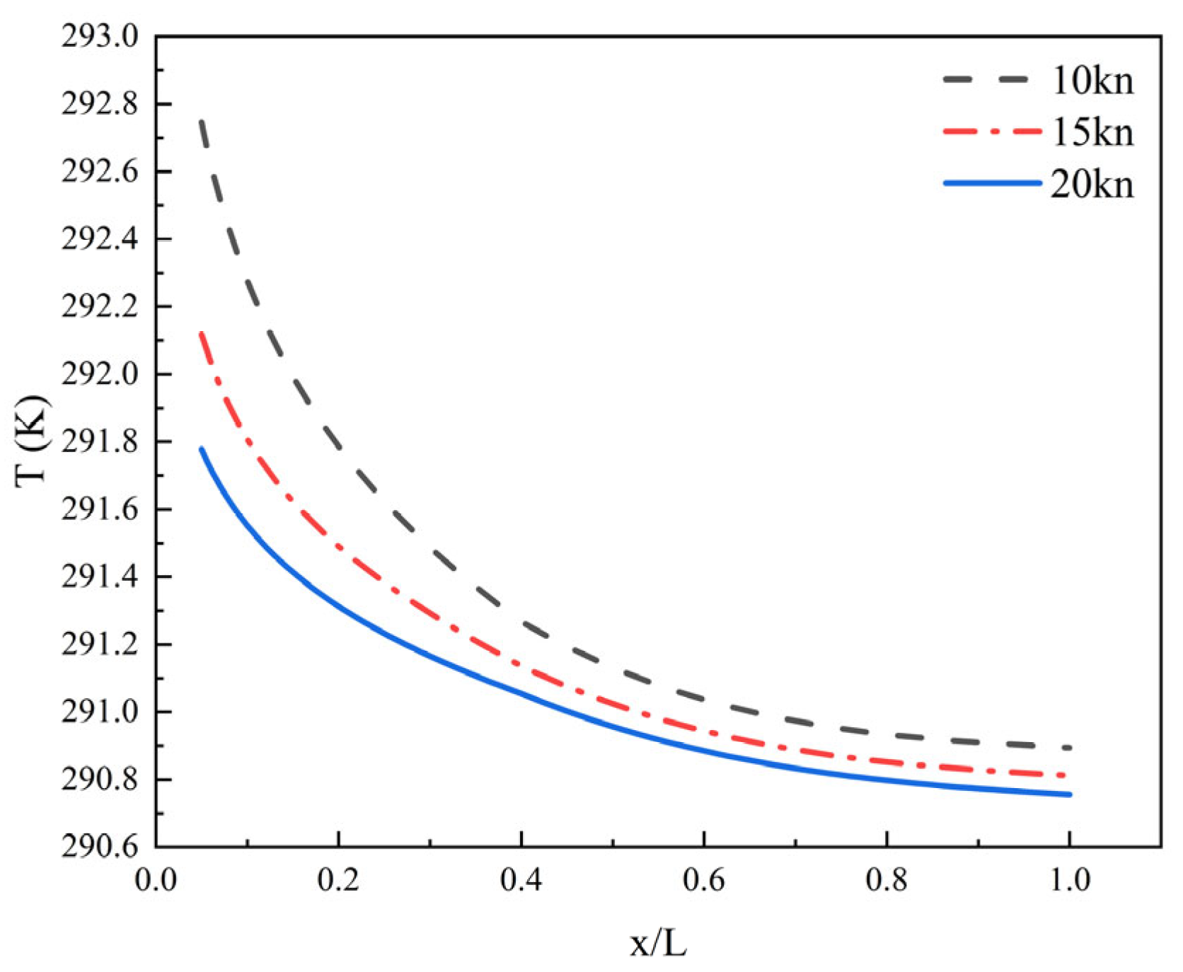
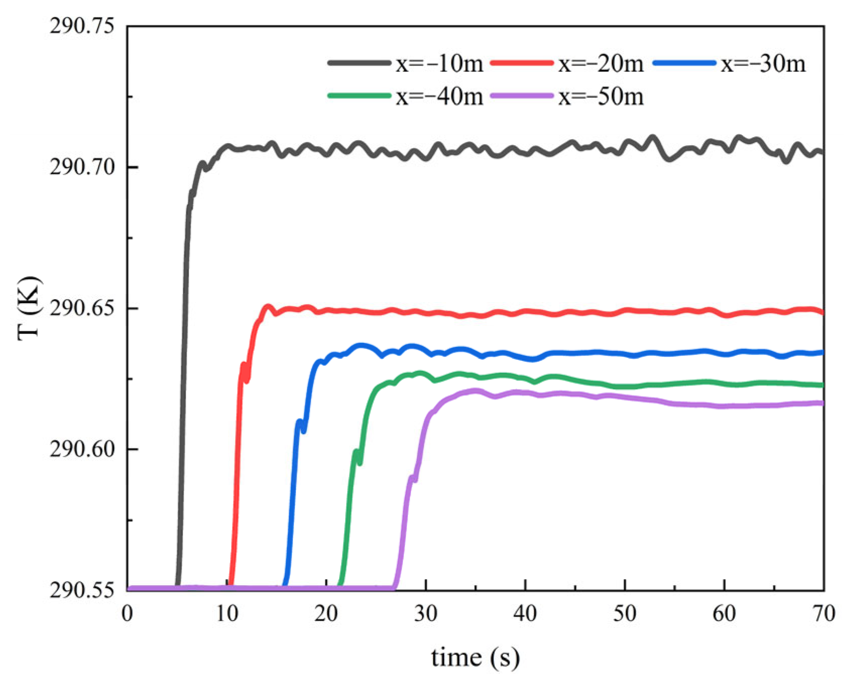
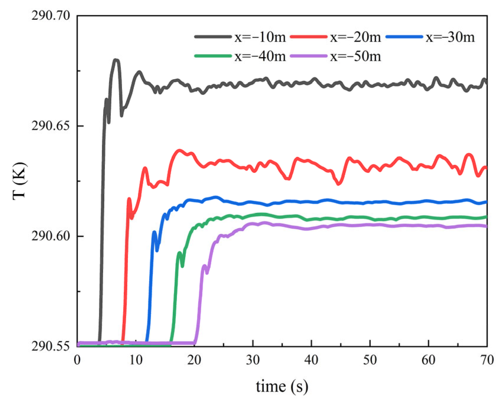
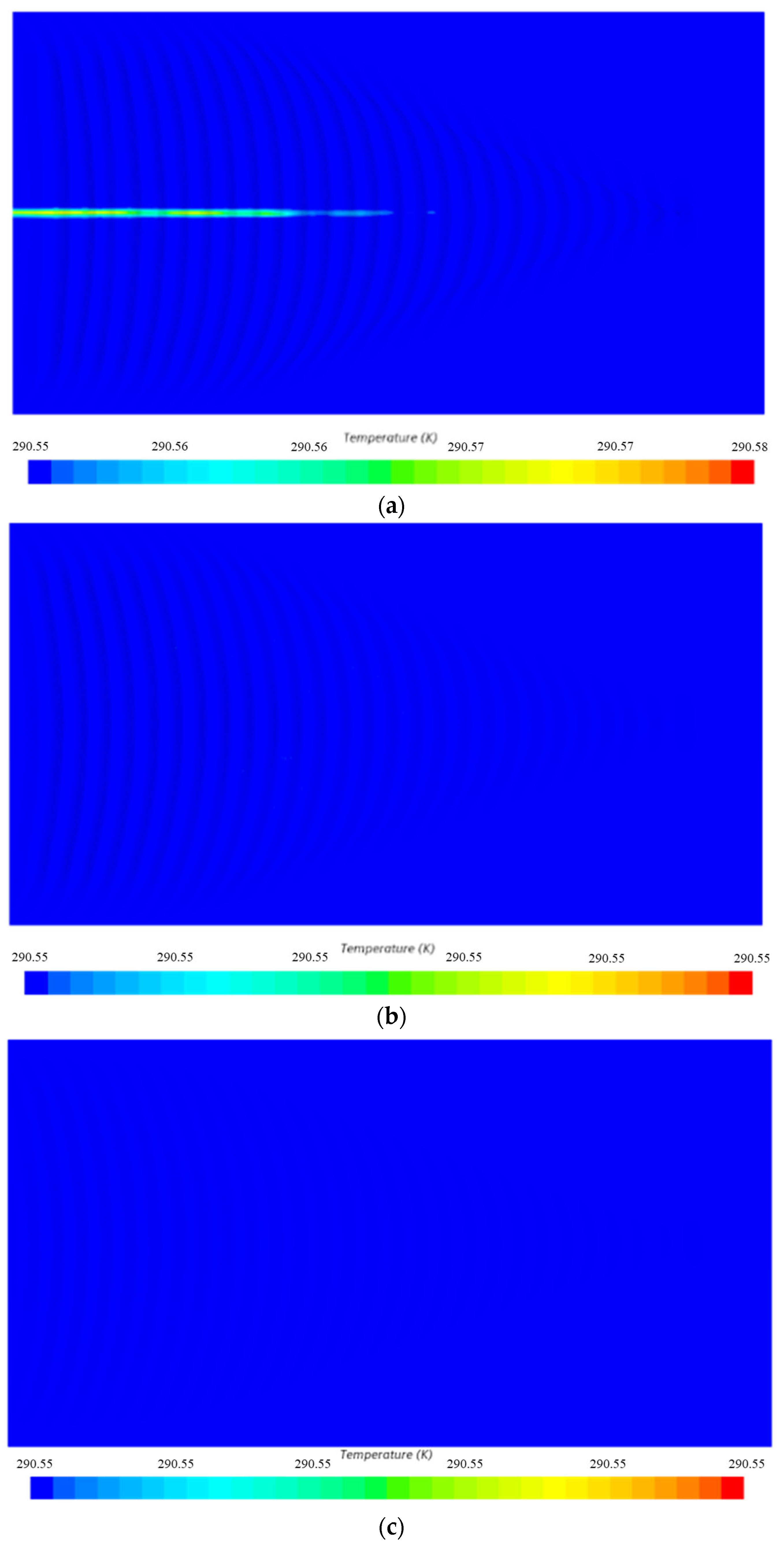
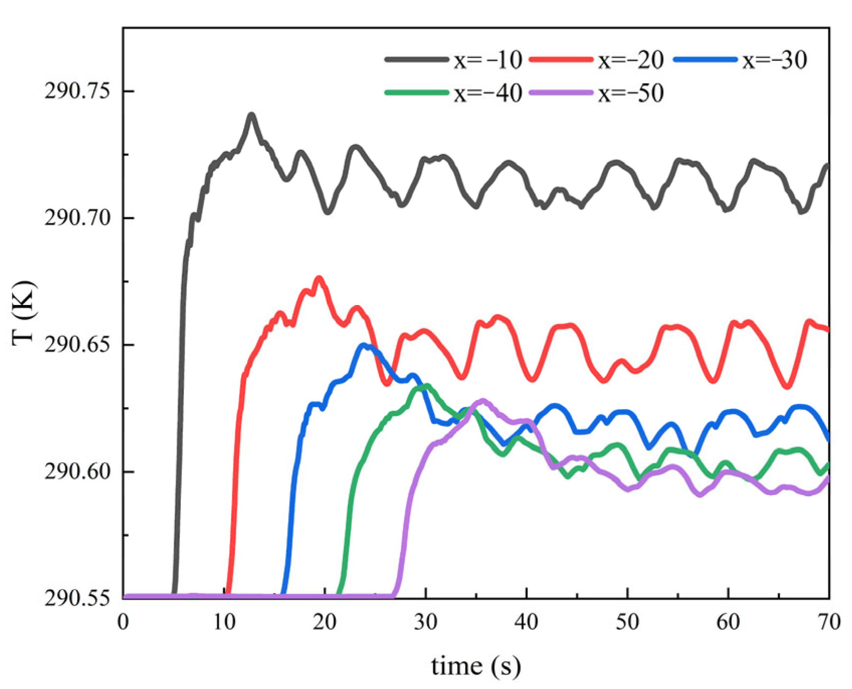
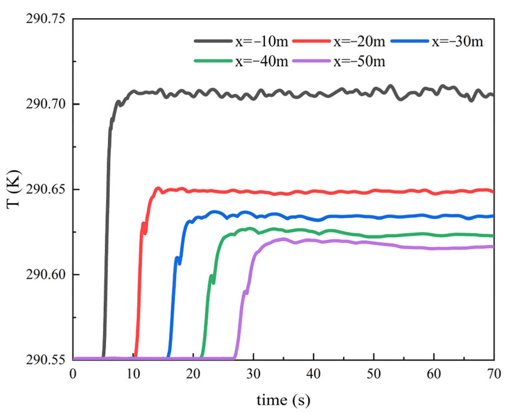
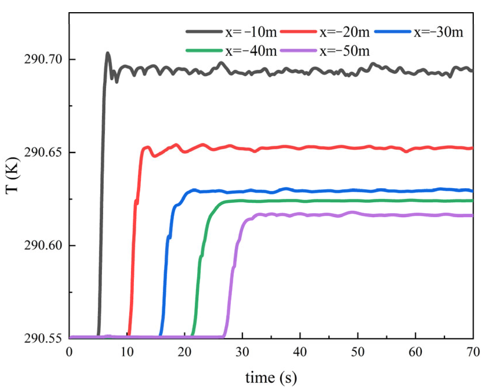
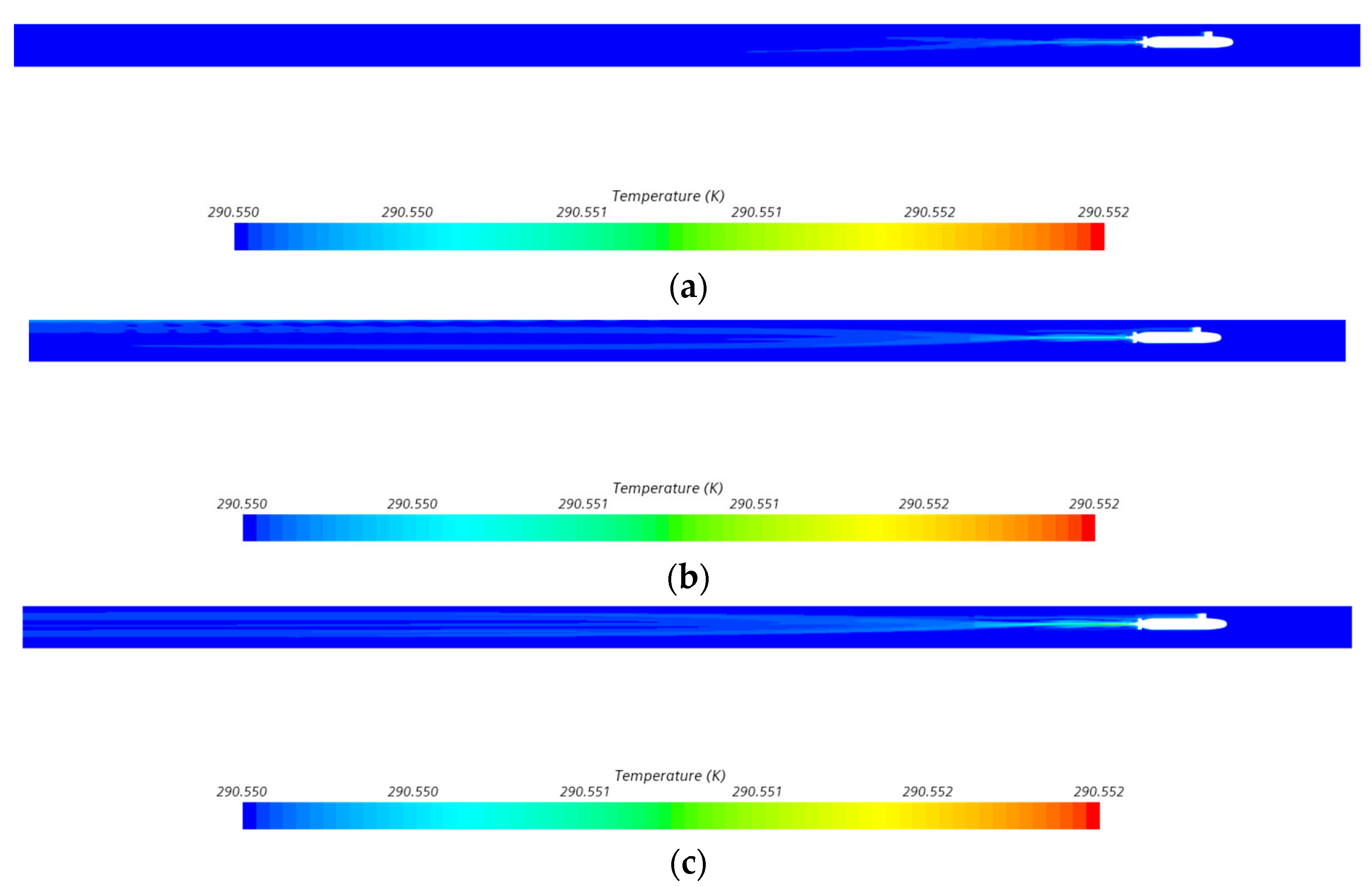
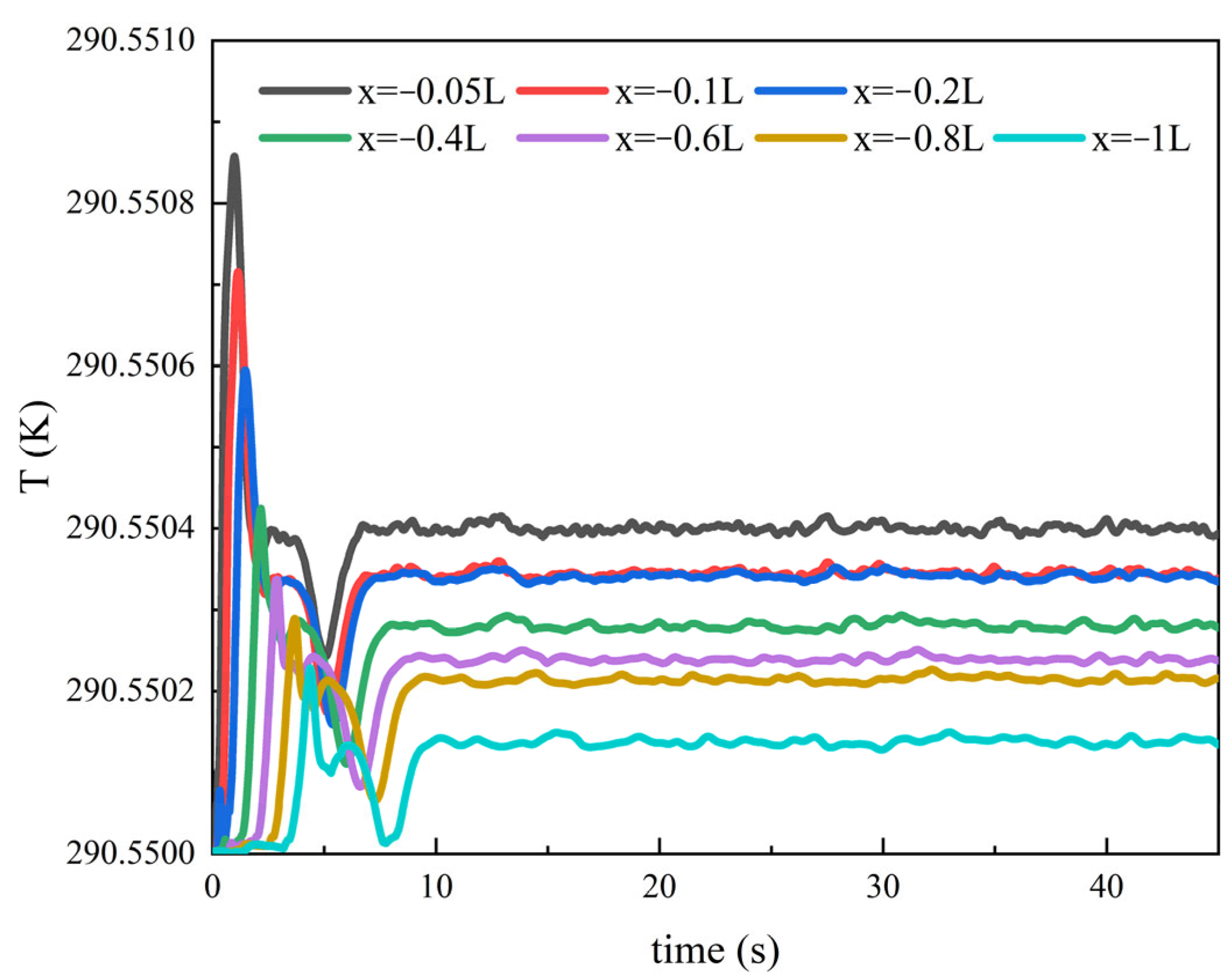
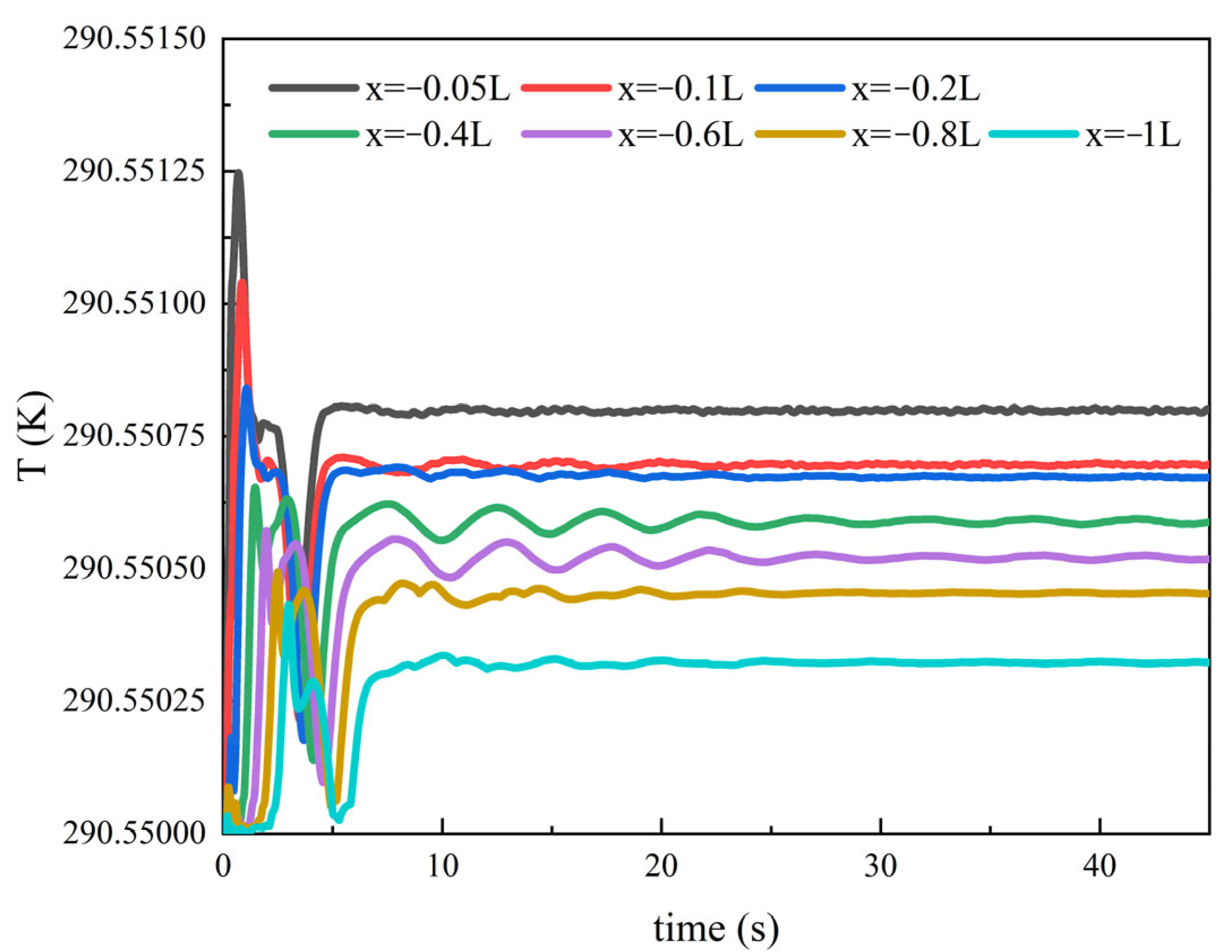
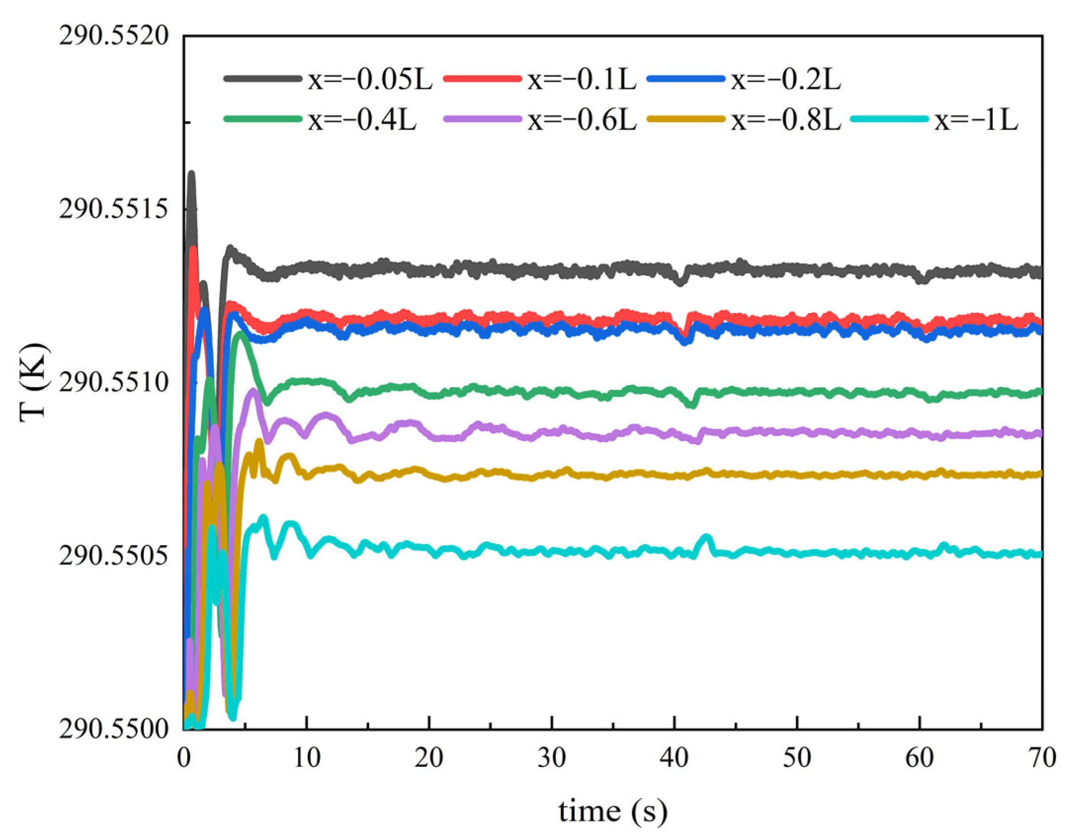
4.3.2. Influence of Speed on Thermal Wake Diffusion Characteristics

The speed also has a great influence on the thermal characteristics of the wake, and the thermal wake shows different characteristics at different speeds. In order to distinguish the near-field and far-field wake thermal characteristics, the range from X = 0 to X = −1 L is taken as the near field, and the range from X = −10 m to X = −50 m is taken as the far field, which is consistent with the definition here in the following paper.
In Figure 20, the calculation time of the flow field is 70 s. Due to the high initial temperature of heat emission, the maximum temperature value is defined as 290.60 K in the figure to clearly show the overall temperature difference on the cross-section. It can be found that at this time, the depth of the thermal feature color bar of the Y = 0 section of the flow field presents a negative correlation law with the speed; that is, the smaller the speed, the more obvious the thermal feature in the wake field. The law is more clear when multiple cross-sections are taken from the flow field.
As can be seen from Figure 21, the higher the speed, the stronger the disturbance of the underwater vehicle to the seawater, and the faster the rotational speed of the propeller, both of which will intensify the diffusion effect of the hot wake, and the heat exchange between the high-temperature and the low-temperature seawater becomes more intense. Therefore, the higher the speed, the lower the wake temperature.
In this paper, the time–history curves of the maximum temperature of different cross-sections in the near field and far field are calculated, and the changes in the maximum temperature of different cross-sections and the changes in wake temperature with the sailing distance can be intuitively seen. Figure 22, Figure 23, Figure 24 and Figure 25 show the variation in the near-field wake temperature of an underwater vehicle.
As can be seen from Figure 22, Figure 23, Figure 24 and Figure 25, with the passage of calculation time, the maximum temperature of each section increases first and then drops back to a relatively stable temperature value, and the convergence curve presents a certain oscillation phenomenon. Figure 22 shows the near-field wake temperature at different speeds, and it summarizes Figure 23, Figure 24 and Figure 25. The presented law is consistent with the flow field temperature cloud map, and the results are intuitive. The higher the speed, the lower the temperature value, and the temperature value first shows a phenomenon of a sharp decline and then a slow decrease in the X direction. This paper also calculates the temperature curve of the far-field wake. Figure 26, Figure 27 and Figure 28 show the temperature variation of the far-field wake of the submersible.
Similar to the near-field wake temperature, as the calculation time goes on, the maximum temperature of each section of the far field also first presents a rise and then converges to a relatively stable temperature value. Unlike the near-field temperature, the oscillation phenomenon of the convergence curve is not very obvious. Figure 29 shows the far-field wake temperature at different speeds, and it summarizes the temperature from Figure 26, Figure 27 and Figure 28. The presented law is basically the same as that of the near-field temperature. The higher the speed, the lower the temperature value, and the temperature value shows a phenomenon of a sharp decline first and then a slow decrease in the X direction. This slowly decreasing temperature indicates that the thermal wake will exist for a long time in the flow field, so the thermal emission of the submersible has a great influence on its concealment.

4.3.3. Influence of Submersible Depth on Hydrodynamic Wake Characteristics

Numerical calculations were performed for the operating conditions in Table 2 with depth as the variable, specifically conditions 3, 4, and 6, where the submarine’s speed was fixed at 15 knots. The wave generation on the water surface for each condition is shown in Figure 30, Figure 31 and Figure 32.
At a fixed speed of 15 kn, the free-surface wake patterns vary markedly with submergence depth. At 10 m depth, the Kelvin wake is strongest: wave crests are sharp and high-amplitude, and the wake extends far downstream. At 20 m depth, the surface disturbance is noticeably weaker—crest heights are reduced, the visible wave train is shorter, and energy decays more rapidly. By 30 m depth, the free-surface response is further attenuated: crests are low in amplitude and largely confined to the immediate vicinity of the hull, and the downstream wake signature is almost lost. This progression illustrates how increasing depth diminishes the pressure disturbance reaching the surface and thus weakens the visible wave pattern.
Figure 33 shows the comparison of wave heights of different deep water surfaces under a Kelvin wave angle of 19°28′, and the measured parameters are consistent with the conditions of different speed mentioned above. Through comparison, it is found that there is a negative correlation between the water surface wave height and submersible depth in this range; that is, the lower the submersible depth is, the higher the wave surface is, and the more obvious the wave surface. The wave height is similar to that obtained by changing the speed above, but the wave wavelength shows a completely different rule. It can be said that the wave wavelength that can be captured on the water surface basically remains unchanged regardless of the change in the depth of the dive, which also proves that the wavelength of the water surface is only related to the speed of sailing and has nothing to do with the depth of the dive.
When the submersible speed is 15 kn, the specific dissipation rate and turbulence intensity of the flow field extracted at 1 m behind the central axis and at the transversal surface of the underwater vehicle are shown in Figure 34 and Figure 35. The specific dissipation rate curve in 33 differs greatly in the range of the ship body, showing a negative correlation with the depth of submersion; that is, the greater the depth of submersion, the greater the specific dissipation rate. However, the difference in the specific dissipation rate of the three depths of the tail of the submersible is not large, which is because the propeller speed is very fast and the disturbance to the wake field of the three depths is very severe. At this time, the effect of the depth on the specific dissipation rate is very small compared to the propeller. In Figure 35, there is little difference in the turbulence intensity after the bow and tail rudder at the three submersible depths, but the turbulence intensity at the parallel midbody of the submersible also increases with the increase in submersible depth. Therefore, the impact of submersible depth on the specific dissipation rate and turbulence intensity is slightly less than that of speed.

4.3.4. Influence of Depth on Thermal Wake Diffusion Characteristics

In this study, the influence of speed on thermal wake diffusion is mainly reflected in the maximum temperature of different cross-sections below the water surface, that is, speed mainly affects the axial temperature, but the influence of depth on thermal wake is different from that of speed, and it mainly affects the vertical temperature in general.
As can be seen from Figure 36, when the submersible depth is 20 m, wake heat characteristics cannot be observed on the water surface of the flow field. When the submersible depth is 10 m, there is an obvious thermal wake phenomenon on the water surface, and the temperature difference between it and the background flow field even reaches 0.03 K. Infrared technology can easily capture the temperature difference in this range, which is very threatening to the concealed navigation of the submersible. There are many situations in which the submersible releases high-temperature cooling water, and most of them are in the situation of low speed near water. Therefore, this paper also carries out simulation calculations for the situation of low speed at a depth of 10 m, and the value of low speed is 5 kn.
The water surface in Figure 37 also shows a very obvious thermal wake phenomenon. Although the water surface is relatively calm at this time, the wave can hardly be seen. However, the width range of the thermal wake is even larger than that of the speed, 15 kn, and the color bar is more obvious, so it is not conducive to the concealment of the underwater vehicle when sailing near the water surface at a low speed.
In this study, the influence of depth on the temperature of different sections under water is less than that of speed, and the specific influence is mainly reflected in the far-field wake temperature.
Figure 38, Figure 39, and Figure 40 show the temperature time–history curves of different sections in the far field at a depth of 10 m, 20 m, and 30 m, respectively. Taking the far-field section where X = −10 m as an example, the maximum temperature of the section decreases with the increase in the depth of the dive. The depth of the dive is negatively correlated with the maximum temperature of the section. The temperature value of the section where X = −20 m also proves the law. However, when the distance increases to X = −30 m, the temperature value at a depth of 10 m will deviate from the law. The temperature values of both depths 20 and 30 remain the same until X = −50 m. According to the research, when the submersible depth is 10 m, the high-temperature cooling water discharged by the submersible has been diffused to the free water surface at a distance of X = −30 m. At this time, the heat exchange of the hot wake changes from heat exchange between seawater to heat exchange between seawater and air. Underwater, the temperature of the hot wake decreases faster than above the water surface. There is a deviation from the previous rule. Although in this case the thermal wake temperature accelerates reduction, it appears above the water surface, which is not conducive to the concealed navigation of underwater vehicles. Therefore, with reference to the general rule of 20 m and 30 m depth, the greater the depth, the more conducive it is to the concealment of the submersible.

4.3.5. Underwater Vehicle Wake Thermal Characteristics Without Heat Emission

As mentioned above, the thermal emission of underwater vehicles is relatively complicated, but it is not carried out all the time. This section analyzes the simulation results of working conditions 2, 5, and 8. Even if the submersible does not discharge heat, the friction will generate a certain amount of heat due to the disturbance of the main body and the propeller with the seawater, which will also lead to thermal features in the wake.
It can be seen from the above Figure 41 that when the submersible does not carry out heat emission, the higher the speed, the darker the temperature color bar and the higher the temperature value in the wake, which is contrary to the thermal characteristics shown by the wake when there is heat emission. Therefore, this situation confirms the phenomenon of friction heat generation between the propeller, underwater body, and seawater—that is, the higher the speed, the faster the propeller speed; the more intense the interaction between the main body, propeller, and water body; and the hotter the generated heat. The detailed temperature value is shown in the figure below.
Figure 42, Figure 43 and Figure 44 are the time–history curves of the cross-section temperature at different speeds, and Figure 45 is the summary of the previous three figures. It can be intuitively seen that the relationship between the temperature at different sections and speed can be seen, and with the increase in cross-section distance, the temperature decreases continuously and comes closer to the temperature of a steady flow field. At the same time, since the submersible does not carry out heat emission, the temperature difference caused by friction in the wake is very small in numerical value, so the numerical difference of the research on the depth will be smaller. There is little point in discussing this. This paper only summarizes the influence of speed on the characteristics of the thermal wake.

5. Conclusions

In this paper, the energy equation and VOF method are combined to study the turbulent wake and wake thermal characteristics of underwater vehicles. The computational model adopts the SUBOFF model and summarizes the geometric model and simulation numerical model of an underwater vehicle. The numerical simulation of various operating conditions based on different speeds, depths, and levels of heat emission is carried out. The influence of different speeds, depths, and levels of heat emission on the thermal phenomena in the wake is studied, as well as the different characteristics of the thermal wake in the water surface under different depths. This study provides a certain research basis for underwater concealed navigation.
(1) Influence of different speeds on the wake characteristics of the underwater vehicle: An increase in underwater vehicle speed and propeller speed will lead to an increase in wake vorticity. That is, the greater the speed, the greater the wake vorticity at the same distance, and the wave height and wavelength of the water surface are positively correlated with the speed.
(2) Influence of different diving depths on the wake characteristics of the underwater vehicle: There is a negative correlation between dive depth and free-surface wave height. That is, the greater the dive depth, the smaller the free-surface wave height, and the smaller the dive depth, the larger the free-surface wave height. However, there is no significant relationship between wavelength and submersible depth. Regardless of the value of the submersible depth, the wavelength of water surface waves captured by simulation is almost fixed at the same speed.
(3) Influence of different speeds on the wake thermal characteristics of the underwater vehicle: When there is heat emission, the faster the speed, the lower the temperature at the same distance. When there is no heat emission, the faster the speed, the higher the temperature at the same distance. This phenomenon is relatively small.
(4) Influence of different submersible depths on wake thermal characteristics: Compared with speed, the influence of submersible depth on wake thermal characteristics is more manifested on the surface of the water. When the submersible is at a depth of 10 m, the thermal wake phenomenon can be obviously captured on the surface of the water. However, when the depth is more than 20 m, this phenomenon cannot be captured on the surface of the simulated flow field.

Author Contributions

Conceptualization, Y.L., J.C. and B.L.; Methodology, Y.L., B.L. and S.S.; Formal analysis, J.C., S.S. and W.S.; Data curation, W.S., J.C., B.L. and S.S.; Writing—original draft preparation, Y.L., J.C. and S.S.; Writing—review and editing, Y.L., J.C. and W.S.; Supervision, J.C. and Y.L.; Project administration, Y.L., W.S. and B.L.; Funding acquisition, Y.L. and B.L. All authors have read and agreed to the published version of the manuscript.

Funding

This study is supported by the National Natural Science Foundation of China General Project (No. 52171293), the Fundamental Research Funds for the Central Universities (No. 3132025117 and No. 3132023516), Major Program (JD) of Hubei Province (No. 2023BAA023).

Data Availability Statement

The data presented in this study are available in this article (tables and figures).

Conflicts of Interest

The authors declare no conflicts of interest.

Nomenclature

SymbolDescription
ρ ρ Fluid density
u , v , w The velocity components in the Cartesian coordinate system (in the x, y, and z directions)
t Time
x , y , z Spatial coordinates
p Pressure
μ Dynamic viscosity
F x , F y , F z Body force components
T Temperature
c p Specific heat capacity
k Turbulent kinetic energy
S T Energy source term
Γ k The effective diffusion rates of k
Γ ω The effective diffusion rates of ω
G k The turbulent kinetic energy that is generated by the average velocity gradient
G ω The generation of special turbulent kinetic energy dissipation ω
Y k Turbulence k dissipation
Y ω Turbulence ω dissipation
L D D E S Turbulent length scale in DDES

References

  1. Xiao, Y.; Qiu, Z.; Shi, Z. On Current Research Status of UUV and Its Critical Technologies. Electron. Opt. Control 2014, 21, 46–49. [Google Scholar]
  2. Yan, Y. The overview study of non-acoustic detection technology base on UUV application in searching target underwater. Ship Sci. Technol. 2017, 39, 10–13. [Google Scholar]
  3. Wu, M.; Gong, W.; Yuan, B. Study of Surface Temperature Features of Thermal Wake Caused by Underwater Vehicle. Infrared Technol. 2011, 32, 29–34. [Google Scholar]
  4. Wu, M.; Chen, B.; Zhang, X. The Study on the Varied Laws of Surface Feature Parameters Caused by a Going Body Underwater in the Temperature Stratification Ocean. Infrared Technol. 2010, 32, 242–246. [Google Scholar]
  5. Gran, R. An Experiment on the Wake of a Slender Propeller-Driven Body; National Technical Information Service, U.S. Department of Commerce: Springfield, VA, USA, 1973. [Google Scholar]
  6. Schetz, J.A.; Jakubowski, A.K. Experimental Studies of the Turbulent Wake behind Self-Propelled Slender Bodies. AIAA J. 1975, 13, 1568–1575. [Google Scholar] [CrossRef]
  7. Schetz, J.A.; Daffan, E.B.; Jakubowski, A.K.; Cannon, S.; Cox, R.; Dubberley, D. Mean Flow and Turbulence Measurements in the Wake of Slender Propeller-Driven Bodies Including Effects of Pitch Angle; Virginia Polytechnic Institute and State University Blacksburg Department of Aerospace and Ocean Engineering: Blacksburg, VA, USA, 1976; Volume 77, p. 12337. [Google Scholar]
  8. Schetz, J.A.; Daffan, E.B.; Jakubowski, A.K. Turbulent Wake behind Slender Propeller-Driven Bodies at Angle of Attack. AIAA J. 1978, 16, 6–7. [Google Scholar] [CrossRef]
  9. Rudolf, A.; Walther, T. Laboratory Demonstration of a Brillouin Lidar to Remotely Measure Temperature Profiles of the Ocean. Opt. Eng. 2014, 53, 051407. [Google Scholar] [CrossRef]
  10. Hong, F. Numerical simulation of surface wake for submarine moving in homogeneous fluid. J. Ship Mech. 2005, 9, 9–17. [Google Scholar]
  11. Peng, J. Research on diffusion characteristics of submarine thermal wake based on multiphase flow. SHIP Sci. Technol. 2024, 46, 47–52. [Google Scholar]
  12. Chen, S.; Zhong, J.; Sun, P. Numerical Simulation and Experimental Study of the Submarine’s Cold Wake Temperature Character. J. Therm. Sci. 2014, 23, 253–258. [Google Scholar] [CrossRef]
  13. Hu, R. Experimental study on infrared signature of thermal wake of remote control submarine. SHIP Sci. Technol. 2017, 39, 53–56. [Google Scholar]
  14. Zhang, X. The Analysis and Carculation of Infrared Signature of Thermal Wake of Submarines. Laser Infrared 2007, 37, 1054–1057. [Google Scholar]
  15. Luo, H. The Numerical Simulation of Interaction between Free-Surface Wake Generated by a Moving Submerged Body and Stochastic Ocean Waves. J. Shanghaijiaotong Univ. 2007, 41, 1435–1440. [Google Scholar] [CrossRef]
  16. Wang, F. Computational Fluid Dynamics Analysis: Principles and Applications of CFD Software; Tsinghua University Press Co., Ltd.: Beijing, China, 2004. [Google Scholar]
  17. Ferziger, J.H.; Perić, M.; Street, R.L. Computational Methods for Fluid Dynamics; Springer: Berlin/Heidelberg, Germany, 2019. [Google Scholar]
  18. Pan, Y. Analysis on Diffusion Characteristics of Submerged Body Thermal Wake in Ocean Stratified Flow. Master’s Thesis, Harbin Engineering University, Harbin, China, 2020. [Google Scholar]
  19. Spalart, P.R.; Deck, S.; Shur, M.L.; Squires, K.D.; Strelets, M.K.h.; Travin, A. A New Version of Detached-Eddy Simulation, Resistant to Ambiguous Grid Densities. Theoret. Comput. Fluid Dyn. 2006, 20, 181–195. [Google Scholar] [CrossRef]
  20. Huang, T.; Liu, H.L. Measurements of Flows over an Axisymmetric Body with Various Appendages in a Wind Tunnel: The DARPA SUBOFF Experimental Program; British Maritime Technology: London, UK, 1994. [Google Scholar]
Figure 1. The SUBOFF standard model (left) and the large lateral diagonal propeller (right).
Jmse 13 01371 g001
Figure 2. Grid division.
Jmse 13 01371 g002
Figure 3. The result of grid convergence calculation.
Jmse 13 01371 g003
Figure 4. The pressure coefficient of the SUBOFF bare boat.
Jmse 13 01371 g004
Figure 5. SUBOFF geometric models from different perspectives.
Jmse 13 01371 g005
Figure 6. Longitudinal section grid.
Jmse 13 01371 g006
Figure 7. Water surface grid (The black part is the encrypted grid).
Jmse 13 01371 g007
Figure 8. Surface wave generation at a speed of 10 kn.
Jmse 13 01371 g008
Figure 9. Surface wave generation at a speed of 15 kn.
Jmse 13 01371 g009
Figure 10. Surface wave generation at a speed of 20 kn.
Jmse 13 01371 g010
Figure 11. Water surface wave height comparison (Speed 10 kn, 15 kn, 20 kn).
Jmse 13 01371 g011
Figure 12. X = −0.05 L vortex cloud image.
Jmse 13 01371 g012
Figure 13. Eddy current structure extracted by the Q criterion.
Jmse 13 01371 g013
Figure 14. Vortex cloud image.
Jmse 13 01371 g014
Figure 15. Vorticity of different sections at a speed of 10 kn.
Jmse 13 01371 g015
Figure 16. Vorticity of different sections at a speed of 15 kn.
Jmse 13 01371 g016
Figure 17. Vorticity of different sections at a speed of 20 kn.
Jmse 13 01371 g017
Figure 18. Specific dissipation rate at different speeds at depth = 20 m.
Jmse 13 01371 g018
Figure 19. Turbulence intensity curves at different speeds at depth = 20 m.
Jmse 13 01371 g019
Figure 20. Thermal characteristics of Y = 0 cross-section at different speeds at a depth of 10 m: (a) speed 10 kn; (b) speed 15 kn; (c) speed 20 kn.
Jmse 13 01371 g020
Figure 21. Thermal characteristics of cross-section at different speeds and a depth of 20 m: (a) speed 10 kn; (b) speed 15 kn; (c) speed 20 kn.
Jmse 13 01371 g021aJmse 13 01371 g021b
Figure 22. Near-field wake temperature at different speeds.
Jmse 13 01371 g022
Figure 23. Section temperature at speed 10 kn (Near-field).
Jmse 13 01371 g023
Figure 24. Section temperature at speed 15 kn (Near-field).
Jmse 13 01371 g024
Figure 25. Section temperature at speed 20 kn (Near-field).
Jmse 13 01371 g025
Figure 26. Section temperature at speed 10 kn (Far-field).
Jmse 13 01371 g026
Figure 27. Section temperature at speed 15 kn (Far-field).
Jmse 13 01371 g027
Figure 28. Section temperature at speed 20 kn (Far-field).
Jmse 13 01371 g028
Figure 29. Far-field wake temperature at different speeds.
Jmse 13 01371 g029
Figure 30. Water surface wave at depth 10 m.
Jmse 13 01371 g030
Figure 31. Water surface wave at depth 20 m.
Jmse 13 01371 g031
Figure 32. Water surface wave at depth 30 m.
Jmse 13 01371 g032
Figure 33. Water surface wave height comparison (Depth 10 m-black, 20 m-red, 30 m-green).
Jmse 13 01371 g033
Figure 34. Specific dissipation rate for different depths at a speed of 15 kn.
Jmse 13 01371 g034
Figure 35. Turbulence intensity curve for different depths at a speed of 15 kn.
Jmse 13 01371 g035
Figure 36. Water surface thermal characteristics at different depths and a speed of 15 kn: (a) depth 10 m; (b) depth 20 m; (c) depth 30 m.
Jmse 13 01371 g036
Figure 37. Surface thermal characteristics at a speed of 5 kn and a depth of 10 m.
Jmse 13 01371 g037
Figure 38. Different cross-section temperatures at depth 10 m (Far field).
Jmse 13 01371 g038
Figure 39. Different cross-section temperatures at depth 20 m (Far field).
Jmse 13 01371 g039
Figure 40. Different cross-section temperatures at depth 30 m (Far field).
Jmse 13 01371 g040
Figure 41. No heat emission, 20 m depth, and Y = 0 cross-section thermal characteristics at different speeds: (a) speed 10 kn; (b) speed 15 kn; (c) speed 20 kn.
Jmse 13 01371 g041
Figure 42. Section temperature at speed 10 kn (Without heat emission).
Jmse 13 01371 g042
Figure 43. Section temperature at speed 15 kn (Without heat emission).
Jmse 13 01371 g043
Figure 44. Section temperature at speed 20 kn (Without heat emission).
Jmse 13 01371 g044
Figure 45. Near-field wake temperature at different speeds (Without heat emission).
Jmse 13 01371 g045
Table 1. Numerical verification results.
Speed (m/s)Resistance (N)Error %
Numerical SimulationBasin Test
3.045101.0102.21.2
Table 2. Homogeneous dense flow field calculation condition.
uniform flow fieldoperating conditionspeed (kn)depth (m)thermal discharge
11020with
2without
31510with
420with
5without
630with
72020with
8without
Table 3. Errors between numerical values and theoretical wavelengths.
Numerical ValueTheoryError
0.8160.847−0.0370
1.9201.9160.0021
3.5203.3900.0383
Disclaimer/Publisher’s Note: The statements, opinions and data contained in all publications are solely those of the individual author(s) and contributor(s) and not of MDPI and/or the editor(s). MDPI and/or the editor(s) disclaim responsibility for any injury to people or property resulting from any ideas, methods, instructions or products referred to in the content.

