Article

Comparison of Innovative Strategies for the Coverage Problem: Path Planning, Search Optimization, and Applications in Underwater Robotics

by
Ahmed Ibrahim
1,2,
Francisco F. C. Rego
3,4,5,* and
Éric Busvelle
6
1
Instituto Superior Técnico, University of Lisbon, 1049-001 Lisbon, Portugal
2
SeaTech School of Engineering, Université de Toulon, Av. de l’Université, 83130 La Garde, France
3
COPELABS—Centro de Investigação em Computação Centrada nas Pessoas e Cognição, Lusófona University, 1700-097 Lisbon, Portugal
4
CTS—Centro de Tecnologia e Sistemas, UNINOVA-Instituto de Desenvolvimento de Novas Tecnologias, 2829-517 Caparica, Portugal
5
Intelligent Systems Associate Laboratory (LASI), 4800-058 Guimarães, Portugal
6
LIS, CNRS, Université de Toulon, Aix Marseille University, 13007 Marseille, France
*
Author to whom correspondence should be addressed.
J. Mar. Sci. Eng. 2025, 13(7), 1369; https://doi.org/10.3390/jmse13071369
Submission received: 17 June 2025 / Revised: 8 July 2025 / Accepted: 15 July 2025 / Published: 18 July 2025
(This article belongs to the Special Issue Innovations in Underwater Robotic Software Systems)

Abstract

In many applications, including underwater robotics, the coverage problem requires an autonomous vehicle to systematically explore a defined area while minimizing redundancy and avoiding obstacles. This paper investigates coverage path-planning strategies to enhance the efficiency of underwater gliders particularly in maximizing the probability of detecting a radioactive source while ensuring safe navigation. We evaluate three path-planning approaches: the Traveling Salesman Problem (TSP), Minimum Spanning Tree (MST), and the Optimal Control Problem (OCP). Simulations were conducted in MATLAB R2020a, comparing processing time, uncovered areas, path length, and traversal time. Results indicate that the OCP is preferable when traversal time is constrained, although it incurs significantly higher computational costs. Conversely, MST-based approaches provide faster but fewer optimal solutions. These findings offer insights into selecting appropriate algorithms based on mission priorities, balancing efficiency and computational feasbility.

1. Introduction

Locating specific targets in an environment often requires a trajectory generation algorithm to ensure a high probability of detection. This leads us to an important concept which is motion planning or path planning. Geographic information systems, robotics, computer graphics, and other industries all encounter path-planning or motion-planning problems. The problem consists of finding an optimal route that avoids obstacles and achieves a certain goal. Normally, the path’s quality is evaluated based on its Euclidean path length, smoothness, and obstacle-free status. In particular, the coverage problem is considered, which amounts to visiting every point in a defined area within a predefined distance.
Throughout this paper, several covering algorithms are to be discussed and implemented based on the state-of-the-art planning methods and coverage problem mentioned in Section 2. These methods can be classified into standard path-planning methods, e.g., the Traveling Salesman Problem (TSP), Minimum Spanning Tree (MST), etc., and search theory using Optimal Control Problems (OCPs) as in the Koopman search theory [1]. Section 3 discusses the theory behind the TSP, MST, and the OCP. Also, it shows a framework for modeling basic search problems that were established as part of WWII antisubmarine warfare activities and have since been widely used in industrial and tactical applications [2]. Afterwards, the numerical methods that are now available to solve the problem at hand are discussed.
Several implemented algorithms can be found in Section 4 associated with multiple simulations and graphs, and a comparison between the aforementioned algorithms is made according to several key points, e.g., the length of the traversed path and time taken during each path. For the MST problem, two configurations were utilized, which are a square configuration and a hexagonal configuration, to define the path traversed in each algorithm.

Problem Definition

Let Q R 2 be a simply connected rectangular region of interest of area A Q punctured by a finite set of polygonal obstacles O = { O 1 , , O M } . The vehicle is modeled as a point mass whose body-clearance requirements are absorbed into an inflated obstacle set O + obtained via a Minkowski sum with the set of all possible robot configurations. Hence, the planner may treat the robot as a point while still respecting hardware safety distances. We consider, therefore, that the free space is F = Q j = 1 M O j + .
The robot carries a downward-looking sensor with footprint radius r s > 0 . Whenever the robot’s center lies at p F , the sensor covers the disc S ( p ) = { x F | x p r s } .
A coverage path is a finite ordered list of way-points W = { w 0 , w 1 , , w N } F . Straight-line interpolation between consecutive way-points yields a piecewise–linear curve Γ ( W ) = i = 0 N 1 [ w i , w i + 1 ] , where [ w i , w i + 1 ] = { ( 1 λ ) w i + λ w i + 1 λ [ 0 , 1 ] } .
The length of the trajectory is L ( W ) = i = 0 N 1 w i + 1 w i . Define the covered set C ( W ) = p Γ ( W ) S ( p ) , and the uncovered (missed) area A m i s s ( W ) = A Q area C ( W ) .
The planning problem consists of selecting w 1 , , w n such that the uncovered area A miss ( W ) and the length of the path L ( W ) are subject to W F . It is thus a tradeoff between two metrics, and each method assigns more weight to one or the other. In particular, we consider the following methods:
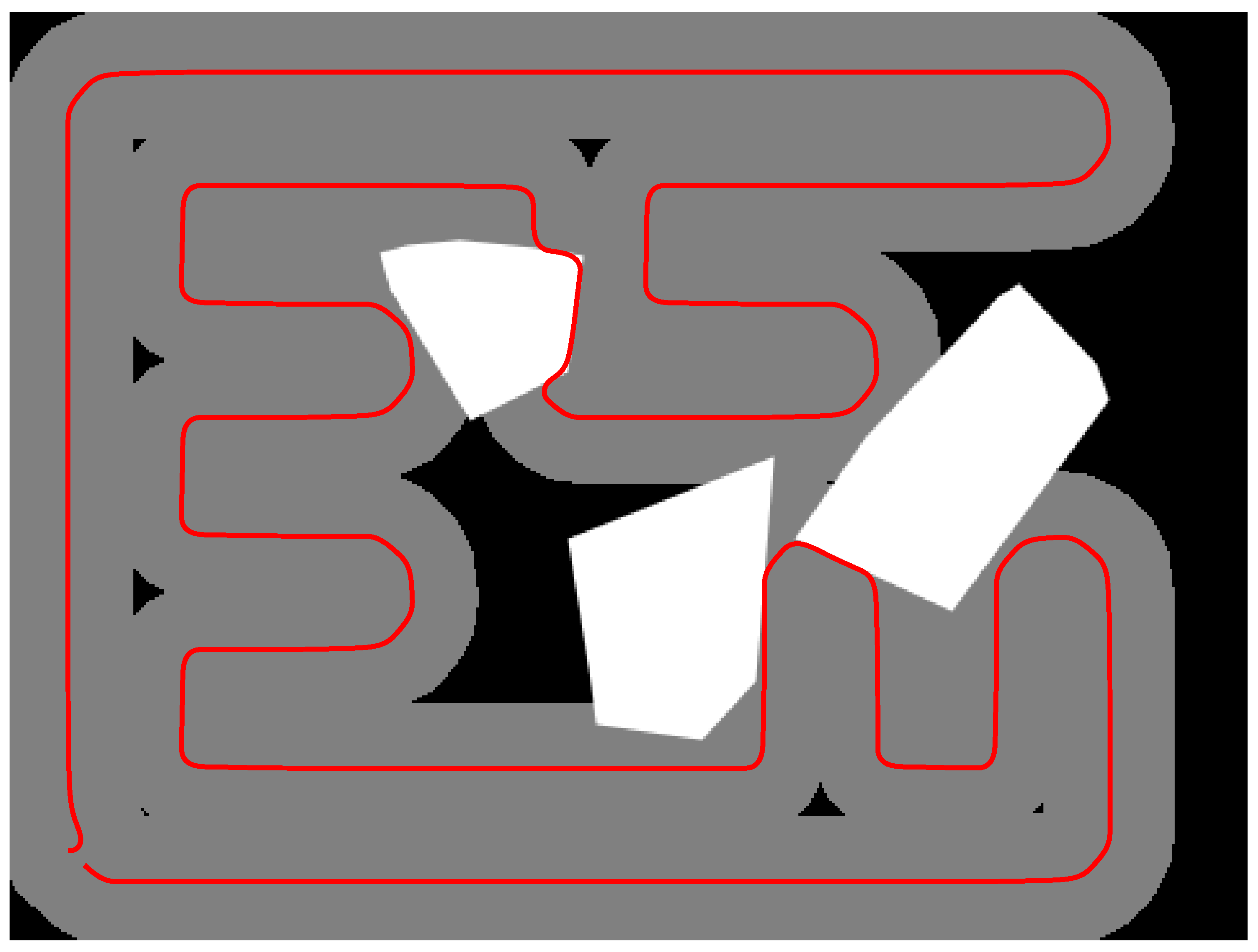
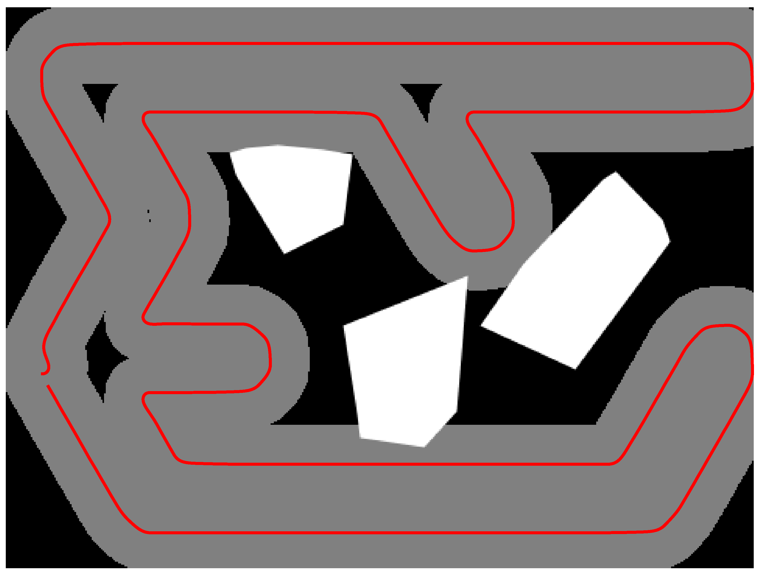
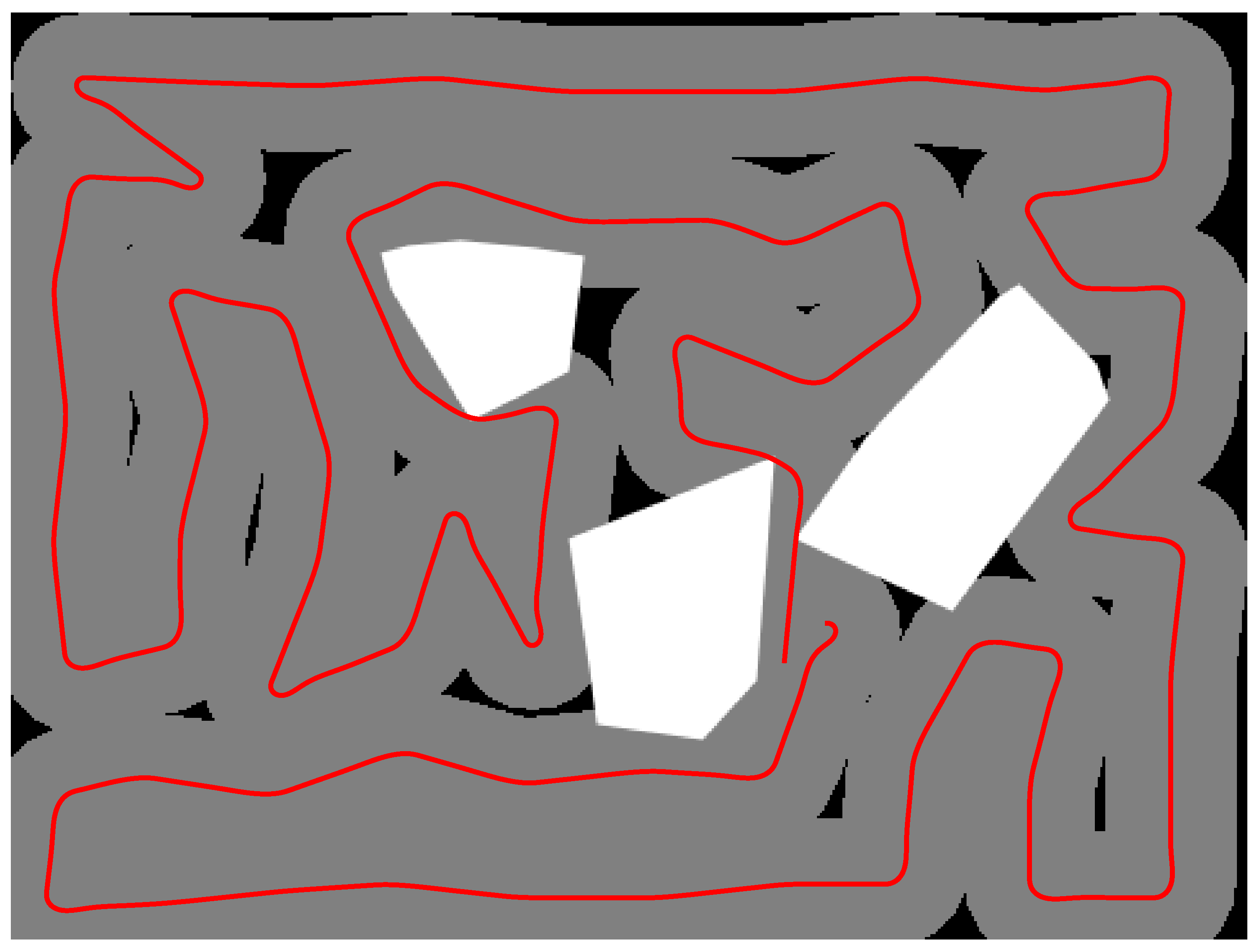
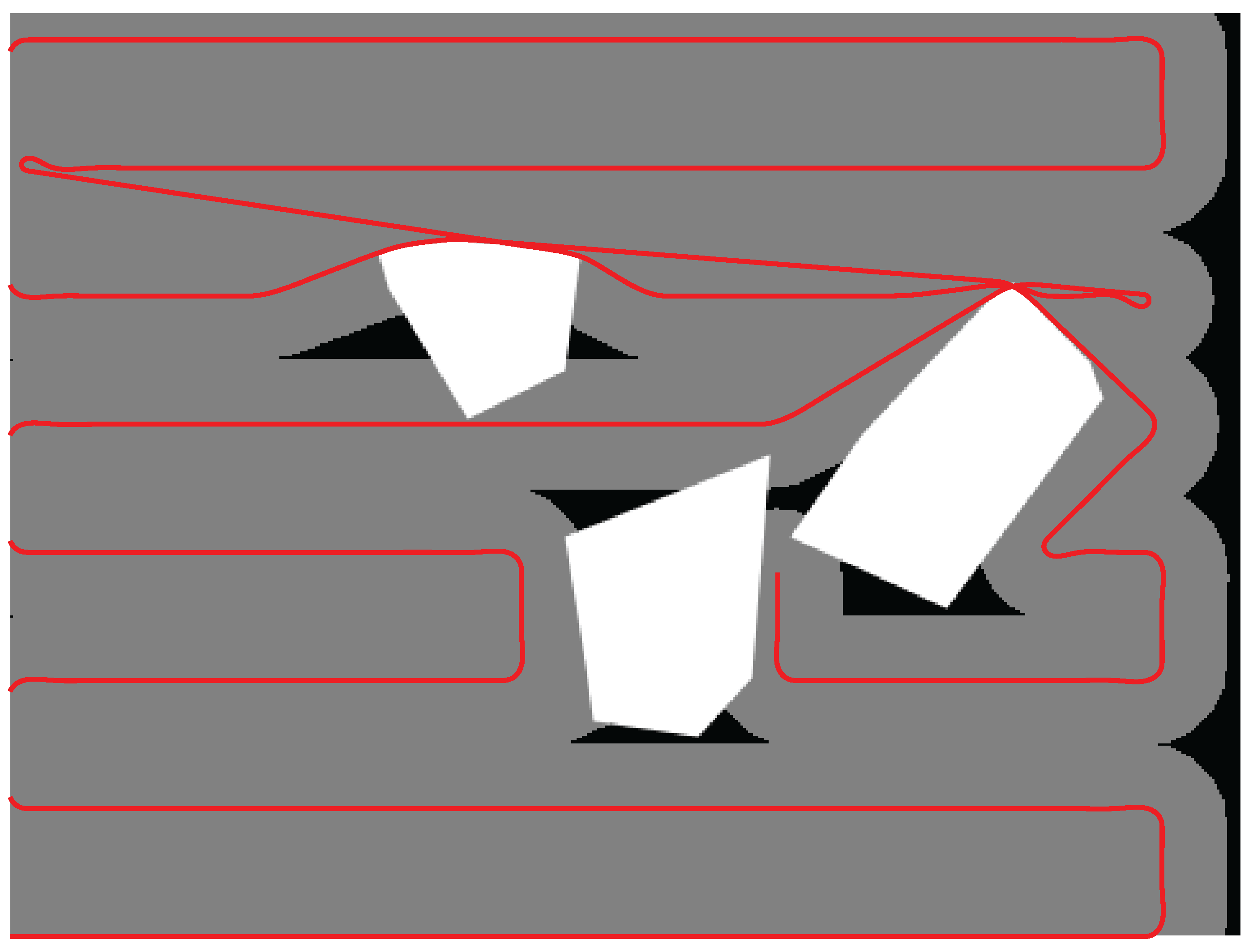
  • TSP path on a point lattice—gold standard for minimum-length tours, but constrained to a fixed selection of way-points, only varying the order.
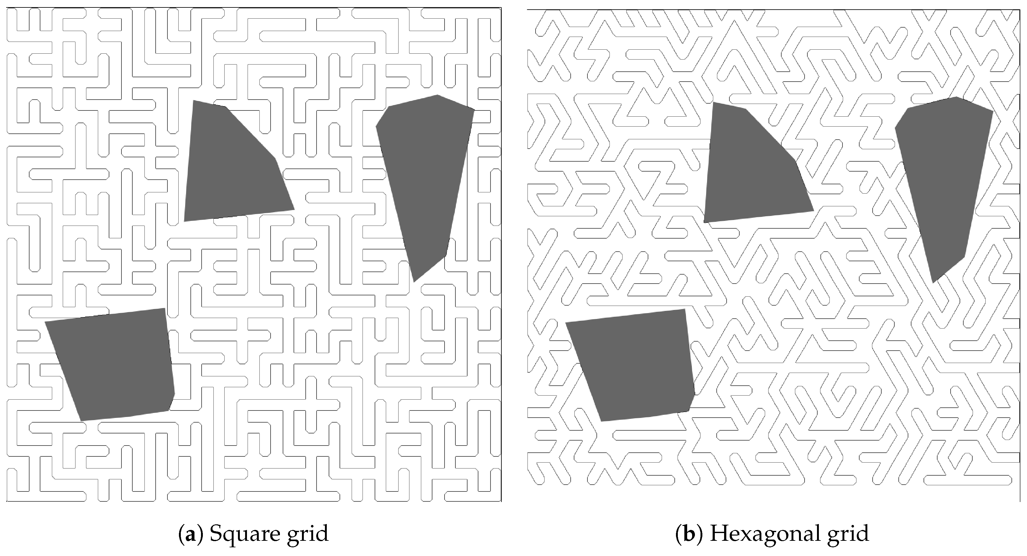
  • MST–Hex and MST–Square—fast, scalable heuristics. The literature lacks a quantitative evaluation of their coverage loss.
  • The OCP [3]—originally formulated for energy-aware path planning, and we adapt it here to address the coverage problem, supplying guidelines for the coverage terms and for warm-starting with TSP.
All planners assume point-mass kinematics after obstacle inflation, meaning every path in our study can be tracked by the physical robot with the same safe margin. Therefore, the comparison is hardware-fair.
Although TSP and MST are standard, the community still lacks a clear answer regarding how much coverage we sacrifice when we pick a sub-second planner (MST) instead of an optimal but slower method (OCP/TSP).
The main objectives of this paper are threefold:
  • Benchmark canonical planners. We deliver a head-to-head quantitative comparison of TSP, MST and an OCP baseline, using the bi-objective metric “uncovered area vs. path length”.
  • Lightweight MST variant for on-board use. There are two key novelties:
    (a)
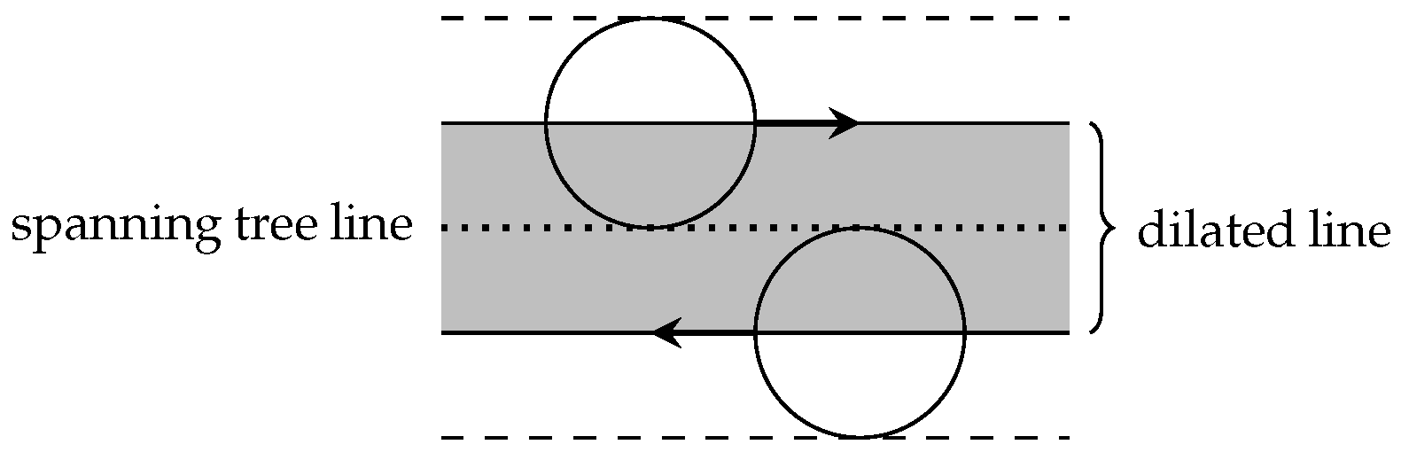
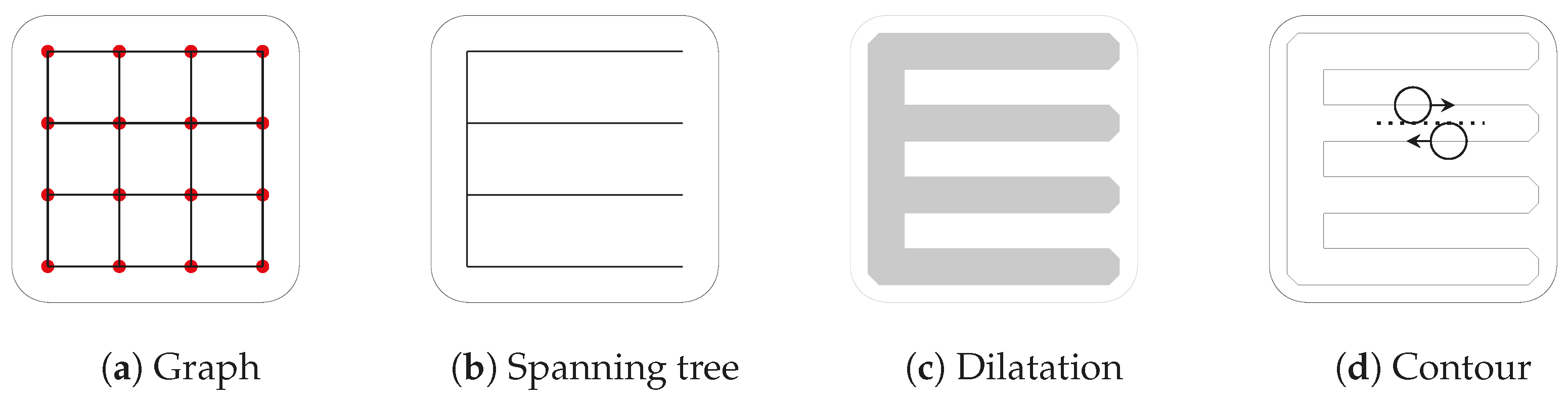
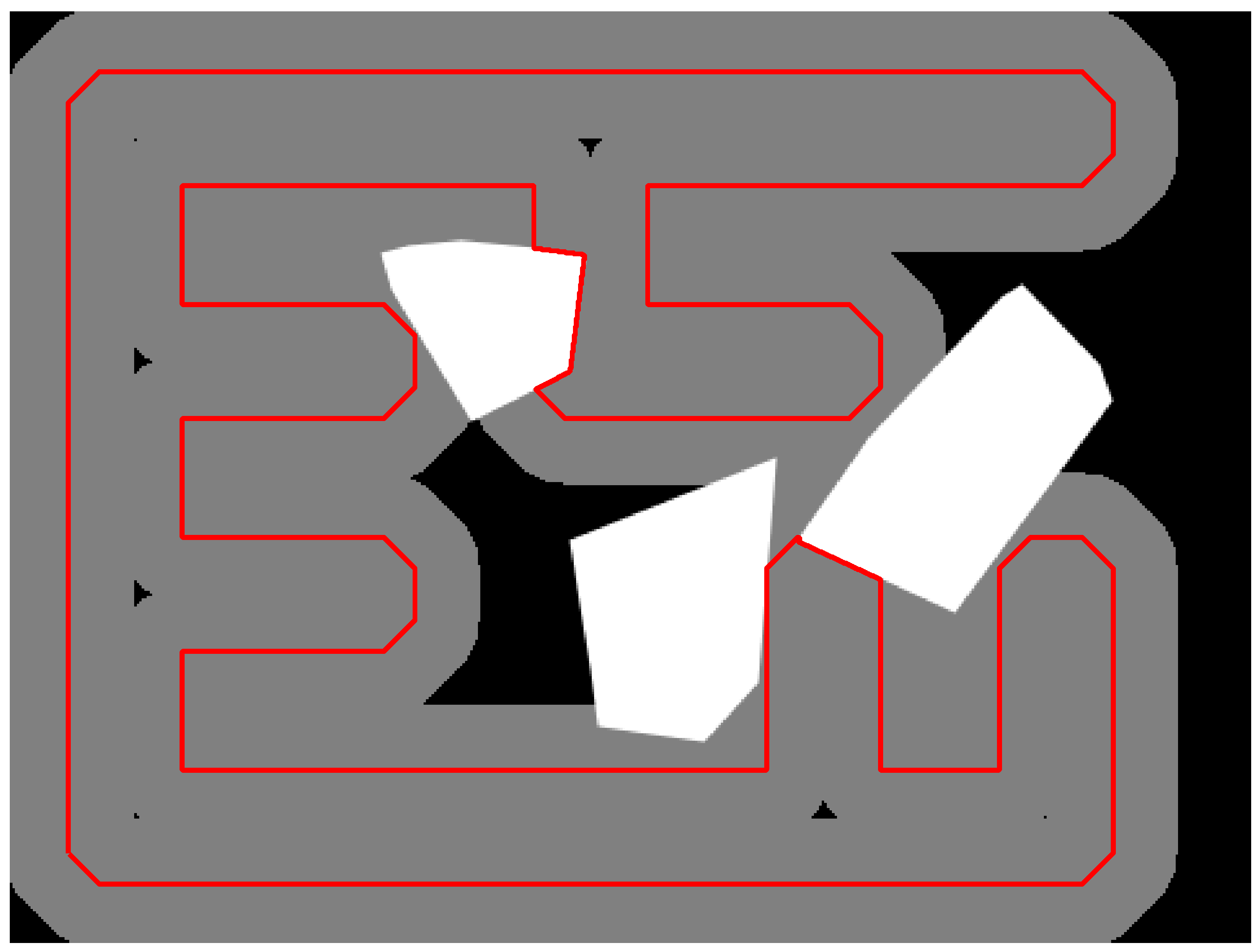
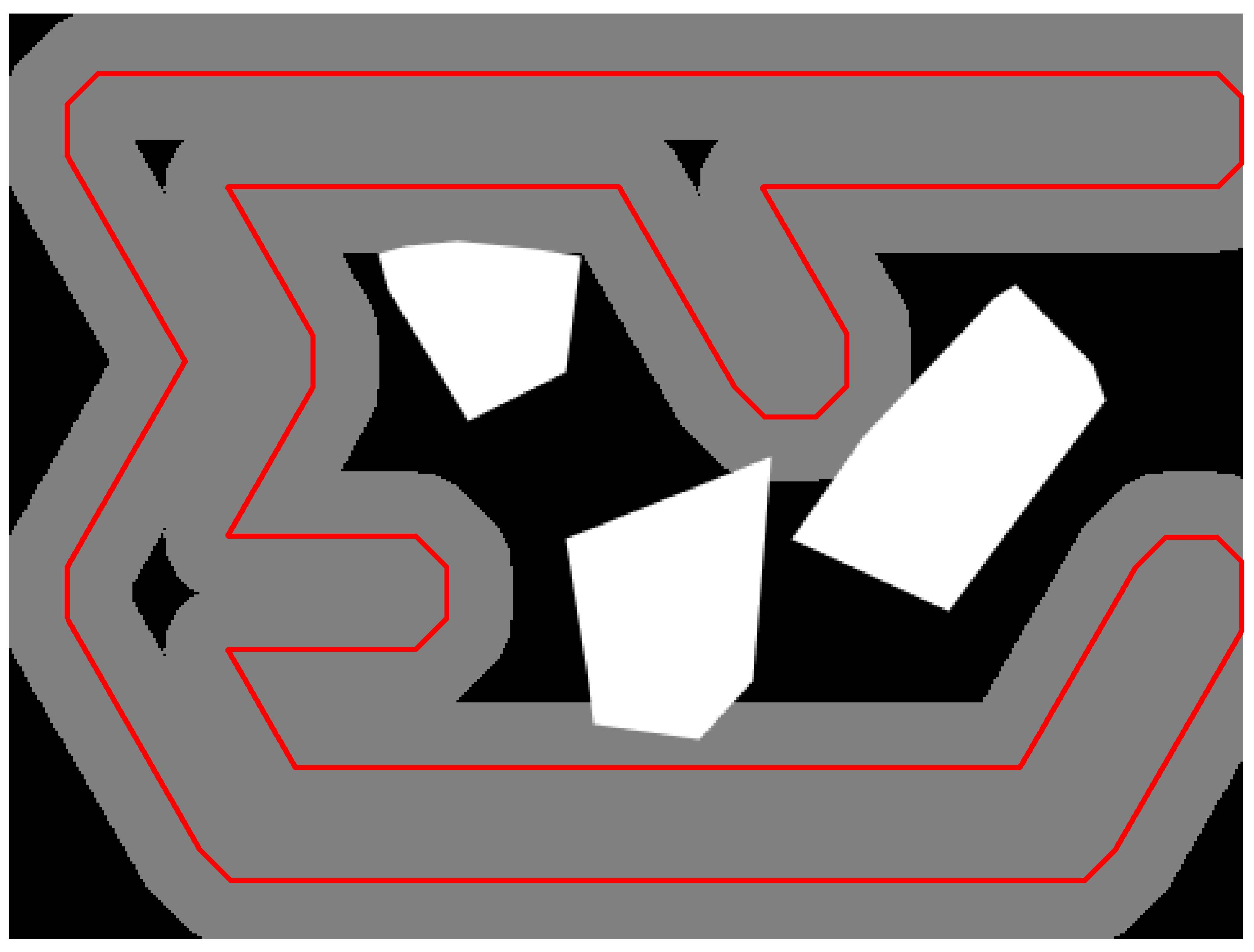
    Tree-to-contour. Dilate the MST and keep its outer boundary, obtaining a single closed sweep line.
    (b)
    Real-time runtime. Coarse grid, Kruskal algorithm, and two image operations complete in under 0.5 s on an Intel i7-12700H.
  • Coverage-tuned OCP. We replace the original energy cost with a “missed-area + path-length” objective, warm-start the solver with the TSP solution, and enforce obstacle constraints directly in the collocation mesh.

2. Literature Review

2.1. Search Theory Problem

Search theory [4] plays a crucial role in the field of robotics, offering a structured approach to solving problems related to navigation, decision making, and resource management. One of its primary applications is path planning, particularly for autonomous robots. By employing search theory, robots can determine the most efficient route to maximize the probability of detecting a determined object while avoiding obstacles and ensuring safe navigation through complex environments.
Moreover, search theory enables the optimization of resources in robotics. Robots often have limited resources, such as energy and computational power. Through the principles of search theory, they can plan their actions to minimize energy consumption and maximize operational time. This is of paramount importance in scenarios where robots are deployed in remote or hostile environments and must operate efficiently with constrained resources.
Furthermore, search theory is useful in exploration and mapping activities. When robots are entrusted with mapping unknown or partially known settings, this theory guides their exploration, allowing them to efficiently map the surroundings and uncover new areas or places of interest. It is essential in applications such as search and rescue, environmental monitoring, and archaeological exploration.
We start with [4], which covers recent advances in pursuit–evasion and autonomous search that apply to mobile robotics applications. Karaman and Frazzoli (2011) [5] discuss sampling-based algorithms for optimal motion planning in robotics. They present algorithms such as Probabilistic Roadmaps (PRMs) and Rapidly-exploring Random Trees (RRTs) that have been shown to work well in practice and have theoretical guarantees of probabilistic completeness. Masakuna et al. (2019) [6] address the problem of search by a group of solitary robots. They propose a coordinated search strategy for self-interested robots without prior knowledge about each other. The results demonstrate the effectiveness of the strategy in achieving efficient search. Ismail and Hamami (2021) [7] conduct a systematic literature review on swarm robotics strategies applied to the target search problem with environment constraints. The review identifies various strategies and highlights their applicability in different research domains, including computational and swarm intelligence.
Yang et al. (2019) [8] propose an extended particle swarm optimization (PSO)-based collaborative searching approach for robotic swarms with practical constraints. The approach aims to address the problem of collaborative search for specific targets in an unknown area. The results demonstrate the effectiveness of the approach in achieving efficient search. Luo et al. (2020) [9] focus on the target search process in swarm robotics. They propose a search approach based on robot chains with an elimination mechanism. The approach utilizes limited perception and the local interaction of robots under a self-organizing mechanism. The results show the effectiveness of the approach in achieving cooperative search. Zhou et al. (2021) [10] propose a multi-target coordinated search algorithm for swarm robots considering practical constraints. The algorithm addresses the challenges of multi-target search in unknown complex environments. The results demonstrate the effectiveness of the algorithm in achieving efficient search.

2.2. Coverage Problem

For several convincing reasons, the coverage problem is extremely important in the realm of robotics. First and foremost, it is critical to efficiently use resources, particularly when resources such as time, energy, or materials are limited. To properly complete their tasks, robots must make well-informed decisions on how to navigate and cover an area. Several researchers consider the covering problem as part of the motion-planning problem.
A critical component related to the coverage issue is time efficiency. Identifying the most time-efficient methods for area coverage is critical in search and rescue missions, inspection activities, and surveillance, especially when time is of the essence. Furthermore, in mobile robotic systems, energy is frequently a valuable and restricted resource. Efficient coverage tactics are critical for reducing energy consumption, prolonging the robot’s operational time, and improving overall efficacy.
The coverage problem guarantees that sensors mounted on robots acquire information equally across the entire region, lowering the danger of missing key data points in data-collecting applications such as environmental monitoring and exploration. In other cases, such as floor-cleaning robots or crop-harvesting equipment, complete coverage is required because missing any part of the area is undesirable.
Furthermore, coverage methods are frequently included in path planning. They aid in the generation of pathways that not only cover the area effectively but also take obstacle avoidance and safe navigation into account especially in dynamic contexts. The coverage problem has several practical applications, including autonomous lawnmowers, vacuum cleaners, agricultural robots, and autonomous cars, all of which require good area coverage to complete their tasks.
The coverage problem in robotics refers to the task of ensuring that one or more robots visit each point in a target area at least once. Several papers have addressed this problem and proposed different approaches and algorithms.
Batalin and Sukhatme (2004) [11] defined the coverage problem as the maximization of the total area covered by a robot’s sensors. They discussed the exploration and deployment of a mobile robot in a communication network and proposed algorithms for efficient coverage.
Galceran and Carreras (2013) [12] conducted a survey on coverage path planning for robotics. They presented a collection of algorithms for complete coverage path planning using a team of mobile robots in unknown environments. They discussed various approaches, including boustrophedon decomposition and cellular decomposition.
Algorithms mentioned by Batalin and Sukhatme (2004) [11] and Le et al. [13] improved the efficiency of coverage path planning. However, resource constraints and coverage optimization were not studied, which was accomplished by Strimel and Veloso (2014) [14].
Classic search theory was conceived for a single agent sweeping a static map; yet today’s robotics problems feature dynamic obstacles, limited onboard computation and swarms of platforms. Recent work illustrates the gap: Khan [15] keeps coverage online but cannot cope with moving obstacles; Huang [16] handles irregular lawns yet still assumes a quasi-static world; and Höffmann [17] optimizes curvature in agriculture at the cost of CPU-heavy mixed-integer layers. New algorithms such as D-STC [18] and Rapid Voronoi CPP [16] push toward real time, but they have not been benchmarked side-by-side against optimal-control formulations on the same metric set. This motivates our unified study: we adopt the Koopman-based detection model, wrap it into an optimal-control program, and pit it against state-of-the-art graph- and swarm-based planners on identical maps.
Equally important is the transition from a path to a trackable trajectory. Hung et al. [19] show that input-constrained path following can guarantee a global region of attraction for marine robots provided the reference path is smooth and curvature-bounded. This can be achieved by post-processing graph-based paths with the smoothing routine in [17]. This ensures every candidate generated in our comparison is not only coverage-optimal in theory but also executable on hardware with limited actuation authority, closing the traditional gap between high-level search theory and low-level control. Most recently, Gkesoulis et al. [20] demonstrated that fusing an obstacle-aware coverage planner with an input-constrained underwater vehicle controller enables reliable, end-to-end seafloor missions in SITL trials—underscoring the value of planning-and-control co-design for realistic deployments. When multiple vehicles are involved, the strategies in [21] may be employed.

2.3. Minimum Spanning Tree

A Minimum Spanning Tree (MST) is a graph tree given by a subset of edges that connects all nodes while minimizing the overall sum of edge weights. In robotics, these nodes can represent critical sites that the robot must visit, and the MST acts as a roadmap for linking these spots effectively. Robots can cross the MST’s edges to visit all essential places while traveling the least amount of distance; see [22].
The spanning-tree coverage has already been described in [23,24]. One of the main interests of this method is its cost in terms of computation time, which is negligible compared to approaches based on approximate resolutions of integer optimization problems, such as the Traveling Salesman Problem (polynomial cost, compared to an exponential cost for the exact TSP algorithm).
This approach can be used for a single robot or for a fleet of N robots. In the latter case, there are several ways to assign the surface to be explored to each robot:
  • The surface can be divided into N areas of equal surface a priori, but this does not guarantee optimality, since some areas can be much more difficult to explore;
  • The problem can be posed and solved for a single robot; then, the trajectory will be divided into N trajectories of equal length, which does not allow for recovering the robots at the place from where they started;
  • Finally, the calculated minimum spanning tree can be divided into a forest of trees (by removing some branches) of the same size, which then allows them to recover N closed trajectories. If N = 2, both robots will be released and recovered at the same point.
There are many articles on the optimal exploration of a terrain with one or more robots. Some are more specifically devoted to the study of this problem for marine robots. In [25], the authors particularly study the transition to real conditions by focusing on practical constraints. A real experiment made it possible to validate the approach on four gliders. In [26], the spanning tree approach is used, but the authors are more particularly interested in the location of the initial grid without questioning the arbitrary choice of a square tiling of the plane. Moreover, although the spanning tree approach is particularly efficient in terms of algorithmic cost, this point is not explored in depth in most articles.

2.4. Traveling Salesman Problem

An alternative casting for the coverage problem can implemented through the Traveling Salesman Problem (TSP) [27]. The TSP belongs to the class of combinatorial optimization problems where the objective is to find the shortest single path that, given a list of cities (or nodes) and distances between them, visits all the cities only once.

2.5. Optimal Control Problem

Optimal Control Problems present themselves in a variety of domains, such as path planning, to determine the control inputs that minimize a given cost function while fulfilling system dynamics and limitations.
There are various types of Optimal Control Problems, depending on the performance index, the type of time domain (continuous, discrete), the presence of different types of constraints, and what variables are free to be chosen. The formulation of an Optimal Control Problem requires the following:
  • A mathematical model of the system to be controlled,
  • A cost function,
  • A specification of all boundary conditions on states and constraints to be satisfied by states and controls, and
  • A statement of what variables are free.
There are various algorithms for solving Optimal Control Problems, such as evolutionary algorithms, shooting method approaches, and others.
Searching for some sources in an environment can be approximated as searching for uncertain targets, as expressed in [28], which has implemented the shooting approach principles. The shooting approach has been depicted in the optimal search problem, created in the 1940s, offering a fundamental framework for motion planning when looking for uncertain targets. The optimal search problem examines how to maximize the likelihood of detecting a non-evasive target with uncertain properties, given the capabilities of the detection equipment and some restrictions on searcher trajectories.
Koopman search theory [1] was first developed during World War II to optimize anti-submarine warfare strategies. Since then, it has been extensively used in tactical and industrial search applications. This work reviews the mathematical foundation of Koopman’s search models and explores modern numerical techniques that enhance their solution methods.

3. Methodology

All the methods discussed aim to solve the coverage problem, which consists of minimizing the path length while ensuring that the entire area is traversed efficiently. Their mathematical formulations differ, but they ultimately contribute to the same goal of optimal coverage.

3.1. Optimal Control Problem (OCP)

The problem of searching for uncertain targets can be formulated as described in [28]. To construct a performance criterion for the optimal search problem, the probability of target detection must be properly modeled. According to the Koopman search theory [1], an exponential detection probability model can be derived, which has since become a fundamental framework in the optimal search literature.
Following Koopman’s seminal result [1], the probability of non-detection decays exponentially with the time integral of a local detection rate. Walton et al. [28] model that rate with a Poisson scan kernel; we adopt their formulation (Equation (2)) and, for numerical robustness, use the smooth arctan cap. Our formulation relies on three simplifying hypotheses: (1) a memory-less sensor, whereby each detection trial is statistically independent of past measurements; (2) a fixed target position; and (3) single-integrator vehicle dynamics, meaning the commanded velocity acts directly as the time-rate of change of the vehicle’s position with no higher-order inertial effects.

3.1.1. Detection Model Implementation

The exponential detection model assumes that the instantaneous detection rate of a target can be accurately represented. Given a searcher’s position at p s ( t ) and a target’s position at p t ( t ) , this detection rate is given by η ( p s ( t ) , p t ( t ) ) , which determines how sensor characteristics affect detection probability. The detection process is assumed to be memoryless, meaning that detection events in different time intervals are independent. A widely used model for defining η ( p 1 , p 2 , t ) is the Poisson Scan Model, used in [28], which describes detection as a probabilistic process influenced by distance and sensor parameters. Under this model, the detection rate function is given by the following:
η ( p s , p t ) = λ Φ F a p s p t 2 σ ,
where λ is a scaling factor representing detection intensity, Φ ( · ) is the cumulative normal distribution function, F is a threshold parameter, a controls the decay of detection probability with distance, and σ is a spread parameter.
The Poisson Scan Model captures sensors whose detection capability decays with range. For coverage planning, though, we prefer an idealized sensor that acts as an indicator function that is constant inside a fixed detection radius and zero outside. For implementation, we adopt the smooth ‘arctan-cap’ approximation of the ideal indicator function. Therefore, the detection rate function is formulated as
η ( p s , p t ) = γ π 2 arctan a p s p t 2 r 2 1 1 π ,
where γ is a scaling factor that controls the maximum detection rate, a is a steepness parameter that determines how sharply the detection rate decreases with distance, and r is the detection radius that defines the detection sensitivity region. This function serves as an approximation of the indicator function of the circle with radius r, that is, when a η ( p s , p t ) approximates
η ( p s , p t ) γ if p s p t < r , 0 if p s p t r .
This function defines how detection probability decays smoothly as the searcher moves further away from the target with a controlled rate of decay dictated by the parameters above.
Under these assumptions, an explicit formula for the probability of target detection is derived. Let P ( t ) denote the probability of non-detection at time t. The independence of time intervals leads to the recurrence equation:
P ( t + Δ t ) = P ( t ) 1 η ( p s ( t ) , p t ( t ) ) Δ t ,
where η ( p s ( t ) , p t ( t ) ) Δ t represents the probability of detection within the interval Δ t , 1 η ( p s ( t ) , p t ( t ) , t ) Δ t is the probability that the target remains undetected, and P ( t + Δ t ) is the updated probability of non-detection at t + Δ t , which is obtained by multiplying P ( t ) by the probability of non-detection in that timestep.
As Δ t 0 , this recurrence relation yields the exponential solution:
P ( t ) = e 0 t η ( p 1 ( τ ) , p 2 ( τ ) , τ ) d τ .
A more general form is expressed as
P ( t ) = G 0 t η ( p s ( τ ) , p t ( τ ) , τ ) d τ .
Throughout this paper, we define G ( x ) as
G ( x ) : = e x .
This formulation ensures that G ( x ) represents an exponentially decreasing probability model, aligning with the Koopman search theory.
Throughout this paper, we consider a deterministic motion model of the searcher p s ( t ) , which assumes that the target’s motion is entirely determined by time. The potential targets are known to belong to a bounded space Ω R n , and their existence follows a known probability density function p : Ω R .
Given a searcher motion p s ( t ) , the probability of not detecting a target P ( t ) becomes a random variable. A natural performance metric is to minimize the expectation of this probability over a time interval [ 0 , T ] , leading to the following cost function:
J = Ω G 0 T η ( p s ( t ) , ω ) d t p ( ω ) d ω .
Using the derivations in [28], Equation (8) can be discrtetized, as shown in Section 3.1.2.
For the coverage problem, we consider a uniform a priori distribution
p ( ω ) = 1 Ω d ω if ω Ω , 0 if ω Ω .

3.1.2. Optimal Control Problem Formulation

The Optimal Control Problem (OCP) aims to determine the optimal trajectory for a system while satisfying dynamic and control constraints.
The system follows a single-integrator model where the state p s ( t ) R 2 evolves according to the control input u ( t ) R 2 :
d p s d t = u .
This means that the control input directly determines the velocity of the system.
The system is subject to the following constraints:
p s ( 0 ) = p s , init , p s ( T ) = p s , final ,
u ( t ) v max , t [ 0 , T ] ,
p s , min p s ( t ) p s , max , t [ 0 , T ] .
The time horizon T is divided into N intervals with a timestep Δ t = T / N . The discretized state and control variables are
p ( s , k ) = p s ( k Δ t ) , u k = u ( k Δ t ) , k = 0 , 1 , , N .
The system dynamics are enforced at each step using an explicit Euler integration:
p s , k + 1 = p s , k + Δ t u k , k = 0 , , N 1 ,
where control and state constraints are imposed at each discretized step.
From the probability formulation, the cost function we wish to minimize is
J = Ω G 0 T η ( p s ( t ) , ω ) d t p ( ω ) d ω ,
we approximate the inner integral with a summation:
0 T η ( p s ( t ) , ω ) d t k = 0 N 1 η ( p s , k , ω ) Δ t .
Substituting this into J,
J i = 1 M G k = 0 N 1 η ( p s , k , ω i ) Δ t p ( ω i ) Δ ω ,
where M is the number of evenly spaced discrete samples of ω .
A penalty function is introduced to ensure the trajectory remains inside the valid search space and avoids obstacles. The penalty is computed as
J penalty = k = 0 N i = 1 M e p s , k O i 2 d 2 ,
where O i represents the positions of obstacles, and d is a threshold defining the avoidance region.
To discourage unnecessarily long paths, a regularization term penalizing the total control effort is included:
J length = λ k = 0 N 1 u k Δ t .
This acts as a soft constraint, pushing the optimization toward minimizing unnecessary deviations.
The overall objective function minimized in the OCP is
J = i = 1 M G k = 0 N 1 η ( p s , k , ω i ) Δ t p ( ω i ) Δ ω + J penalty + J length ,
where the first term represents the primary cost term associated with optimizing search efficiency, and the additional terms enforce obstacle avoidance and path regularization.
This results in a computationally efficient numerical approach to solving the OCP using direct multiple-shooting methods in MATLAB with CasADi [29]. To improve computational efficiency and provide a structured initial guess for the Optimal Control Problem (OCP), the solution obtained from the TSP heuristic is used as an initial trajectory input for the solver. The TSP tour is resampled to N way-points and velocities are set to piece-wise constant vectors between successive points, ensuring feasibility. The optimization problem is then solved using nonlinear programming techniques, ensuring an optimal trajectory while satisfying system constraints. By leveraging the TSP path, the OCP solver benefits from a well-structured initial condition, leading to faster convergence and improved feasibility of solutions.

3.2. Minimum Spanning Tree

We can distinguish several specificities specific to the marine environment:
  • The presence of a third dimension;
  • Winds and sea currents fluctuating over time;
  • The difficulty of navigating certain robots (sailboats, gliders, etc.);
  • The risk of losing a robot (risks of collision, breakdowns, etc.);
  • The specificity of sensors in a marine environment;
  • The difficulty of communicating with fixed stations or between robots when they are underwater.
We will not go into details in this article, because our study is a preliminary work. However, we keep in mind certain objectives in order to overcome the difficulties stated below. Thus, we must generate admissible trajectories, favoring straight lines. But above all, we want to be able to solve the problem very quickly with very limited computing resources so as to recalculate solutions with on-board computing and in real time and subsequently be able to react to disturbances (winds, currents, anti-collision diversion).
We will reformulate the problem as an optimal coverage problem for which we can find a straightforward solution. Rather than maximizing a criterion representing the probability of discovering a source—which intuitively corresponds to meticulously scanning the search area while covering every part—we will explicitly define the problem as finding a path that ensures no point remains at a distance greater than a given threshold, which depends on the sensor’s range. We denote this distance as r. Let us remark that if the probability of detection of the sensor is equal to 1 inside the disk of radius r centered on the sensor and 0 outside the disk, minimizing the probability of non-detection is exactly the same as our reformulated problem.
Thus, the goal is to find a closed path (so that the robot returns to its starting position) that explores a given area in such a way that every point within this area is covered at some moment by the sensor. This is exactly the problem encountered in robotic vacuum cleaners. This type of problem is relatively easy to solve in the case of a rectangular area. To simplify the description, we will assume that the rectangle’s corners are rounded with quarter-circle arcs of radius r (since a robotic vacuum cleaner cannot clean sharp corners, but in our case, this assumption serves merely as a convenient way to explain the algorithm). We will also assume that the lengths of the rectangle’s sides are multiples of 2 r . Again, this assumption simplifies the exposition of the method and helps convince the reader of the method’s near-optimality. Indeed, in this case, the well-known optimal solution is obtained by sweeping the area using a zigzag trajectory; see Figure 1. For a glider-type robot, such a trajectory is particularly interesting because it favors straight-line motion (we will disregard the curvature of the Earth).
The area to be explored is not necessarily rectangular and may not be 1-simply connected. Therefore, the zigzag trajectory must be adapted according to the boundaries and the regions to be avoided. The challenge is thus to develop an algorithm that naturally generates this type of trajectory within a rectangular domain but can also extend to more complex cases.
To achieve this, the surface to be explored is meshed using a 2 r -grid which constitutes a graph G whose intersection points form the vertices; see Figure 2a. Two vertices are connected if they are adjacent in the 4-neighborhood sense. The algorithm, which is straightforward, is as follows:
We first extract a minimum spanning tree (MST) from this graph; see Figure 2b. From a graph–theoretical perspective, we traverse this tree using a depth-first search (DFS). Geometrically, this corresponds to traversing the tree while maintaining a distance r from it. To visualize (and compute) this trajectory, we simply apply a morphological dilation to this graph—interpreted as an image processing operation—with a structuring element of radius r; see Figure 2c. Finally, we extract the contour of the dilated result; see Figure 2d. This contour defines the trajectory to be followed. By construction, it covers the whole space.
The total computational complexity of this algorithm is approximately O ( S r 2 log S r ) , where S is the surface area of the exploration domain:
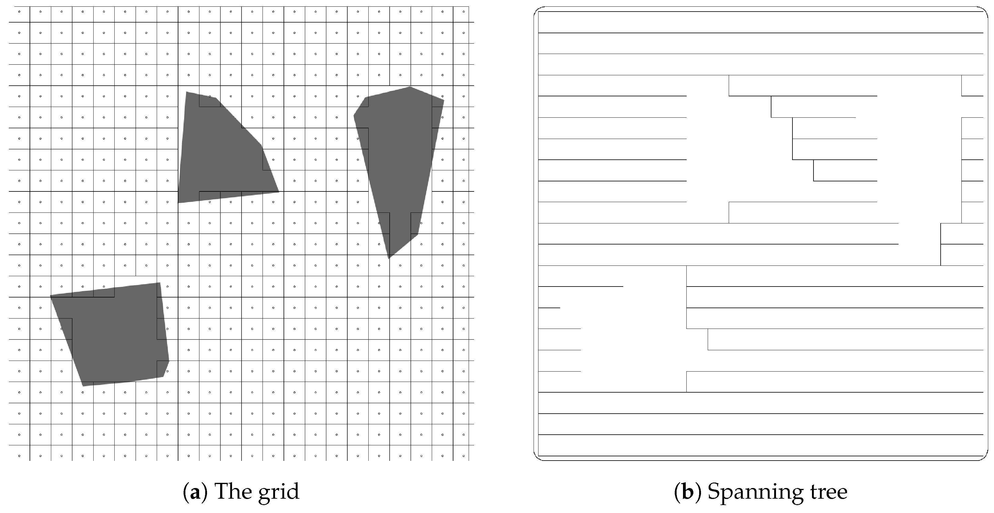
  • The extraction of a minimum spanning tree is performed using Kruskal’s algorithm, which is a greedy algorithm that can be proven to be optimal. It proceeds by sorting the edges in ascending order and iteratively adding them to the tree, ensuring no cycles are formed. Since the number of vertices is proportional to the area to be explored, the number of edges is proportional to the square of this area.
  • The dilation operation is equivalent to a convolution with a disk of radius r. Assuming r is small relative to the exploration area, the cost of this operation is linear with respect to the surface area.
  • Contour extraction can also be formulated as a convolution, for instance, using the Sobel edge detection method, which remains a linear-time operation in terms of surface area. However, to obtain the final trajectory, it is more practical to perform contour following, which can also be executed in linear time.
It is worth noting that throughout this work, we have chosen to favor horizontal over vertical trajectories (in the orientation of our illustrations, this corresponds to east–west rather than north–south on a map—an entirely arbitrary choice). This preference is enforced by introducing a slight penalty on vertical edges compared to horizontal ones before extracting the minimum spanning tree, thereby biasing the solution toward horizontal paths. Geometrically (which becomes relevant if we later opt for a non-grid-based discretization), this corresponds to modifying the Euclidean distance into an anisotropic metric of the form
d = x 2 + ε y 2
where ε is a small penalty parameter. The Euclidean distance provides a less convincing trajectory; see Figure 3, Figure 4, Figure 5 and Figure 6.
The path we compute corresponds to a depth-first traversal of a tree extracted from this graph. Several remarks can be made at this stage:
  • The choice of a grid-based discretization using a rectangular tiling is arbitrary. We have also tested a hexagonal tiling (with centers still at a minimum distance of 2 r ), which may offer advantages for certain spatial geometries in the exploration domain; see Figure 3, Figure 4 and Figure 5.
  • The use of a regular grid ensures minimal-length trajectories in a rectangular domain. However, it may be beneficial to introduce additional points in the discretization to refine exploration in specific areas or to navigate through narrow passages.

3.3. Traveling Salesman Problem

The Traveling Salesman Problem (TSP) [27] is a well-known combinatorial optimization problem. It involves finding the shortest possible tour that visits each city exactly once and returns to the starting point. The TSP can be formulated as an Integer Linear Programming (ILP) problem, where binary decision variables determine whether an edge (i.e., a connection between two cities) is included in the tour.

3.3.1. Problem Statement

Consider a set of n cities C = { 1 , 2 , , n } , where d i j represents the distance between cities i and j. The objective of the TSP is to minimize the total tour length L for a given permutation of cities. In the MATLAB implementation, instead of predefined cities, nodes are sampled on a regular grid, and obstacles are incorporated by removing points that lie within them.

3.3.2. Objective Function

The total tour length L is expressed as the sum of the distances traveled between consecutive cities in the tour:
L = i = 1 n j i d i j x i j .

3.3.3. Constraints

To ensure a valid tour, the following constraints are imposed:
j i x i j = 1 , i C
i C x i j = 1 , j C
i S j S x i j 1 , S { 1 , 2 , , n } , S , S C
Equation (24) ensures that each city is visited exactly once, while Equation (25) ensures that the salesman leaves each city exactly once. Equation (26) prevents subtours that do not include all cities.
Similar to the Minimum Spanning Tree (MST), vertices are selected at a specified distance; however, in the TSP, the distance is set to 0.5 d instead of d. The MATLAB implementation constructs a graph representation of TSP rather than explicitly solving an ILP. Nodes are sampled on a mesh grid, and edges that intersect obstacles are penalized with a large distance to prevent infeasible routes.

3.3.4. Implementation Considerations

In the MATLAB implementation, obstacles are incorporated by removing grid points that lie within them. The edges of the graph are filtered to eliminate paths that intersect obstacles by assigning them a high penalty distance. Instead of an ILP formulation, a distance matrix is constructed, and the TSP solution is found using a heuristic search algorithm.
The solver applies a nearest neighbor heuristic to construct an initial tour, which is followed by 2-opt heuristics to improve the solution. The starting points for the nearest neighbor tour are randomly selected to explore different initial conditions. The 2-opt method iteratively swaps pairs of edges to reduce the total tour length, ensuring a more optimized route.
The objective function in TSP seeks to minimize the total distance traveled while ensuring each node is visited exactly once and the tour returns to the starting point:
Minimize i = 1 N j = 1 N c i j · x i j
where N represents the number of nodes, c i j is the distance or cost between nodes i and j, and x i j is a binary decision variable indicating whether travel occurs between nodes i and j. In practice, the MATLAB implementation avoids an explicit ILP solution and instead constructs a feasible graph representation, solving for an approximate shortest path using heuristics. The heuristic approach follows a well-established method combining nearest neighbor initialization with 2-opt optimization. This approach is widely recognized in TSP research, particularly in heuristic solvers [30].

4. Numerical Results

This section presents results from a single reference map (for illustrative trajectories) and summarizes the average performance of four algorithms (TSP, MST-hex, MST-square, and OCP) and a recent boustrophedon-based method adapted from [15] over 10 randomly generated samples. Each algorithm aims to cover the environment efficiently subject to obstacle constraints and sensor detection capabilities. The code used to obtain the results can be found in github.com/ffcrego87/cover_planning (accessed on 7 June 2025) [31].

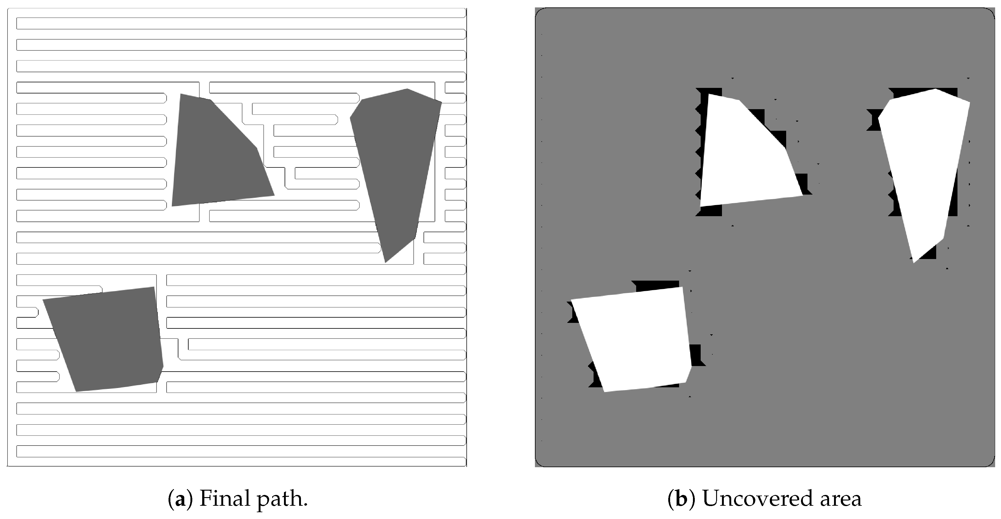
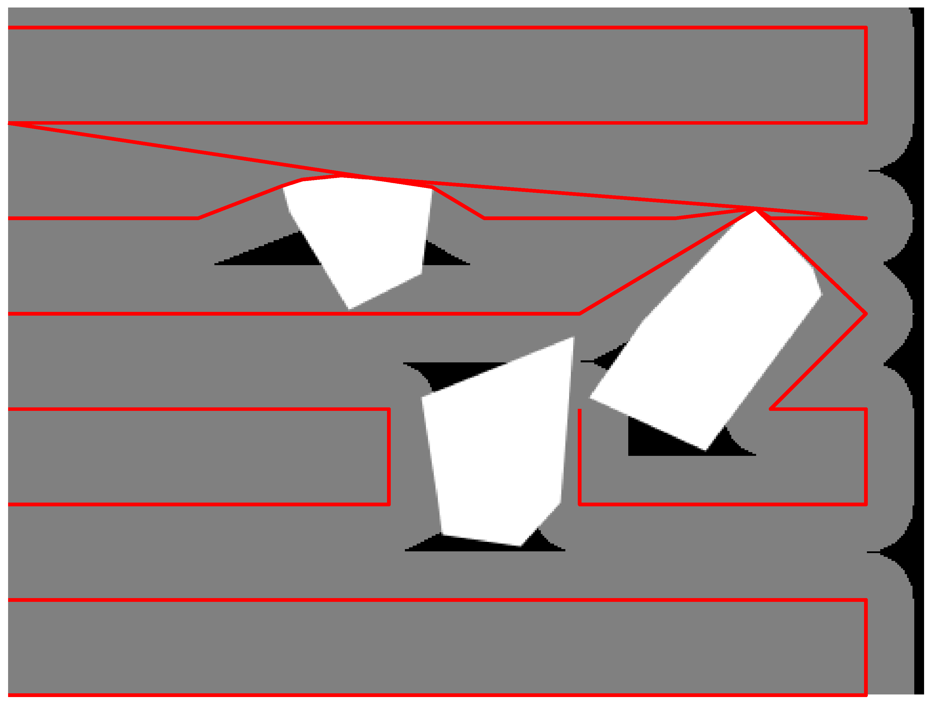
4.1. Single-Sample Illustration

Figure 7, Figure 8, Figure 9, Figure 10 and Figure 11 display representative paths for the MST algorithm with a squared grid configuration, the MST algorithm with a hexagonal grid configuration, the TSP algorithm, the OCP approach, and the boustrophedon approach in [15]. Although these particular trajectories come from one selected map, the subsequent performance metrics are aggregated from 10 runs with distinct randomly generated maps.

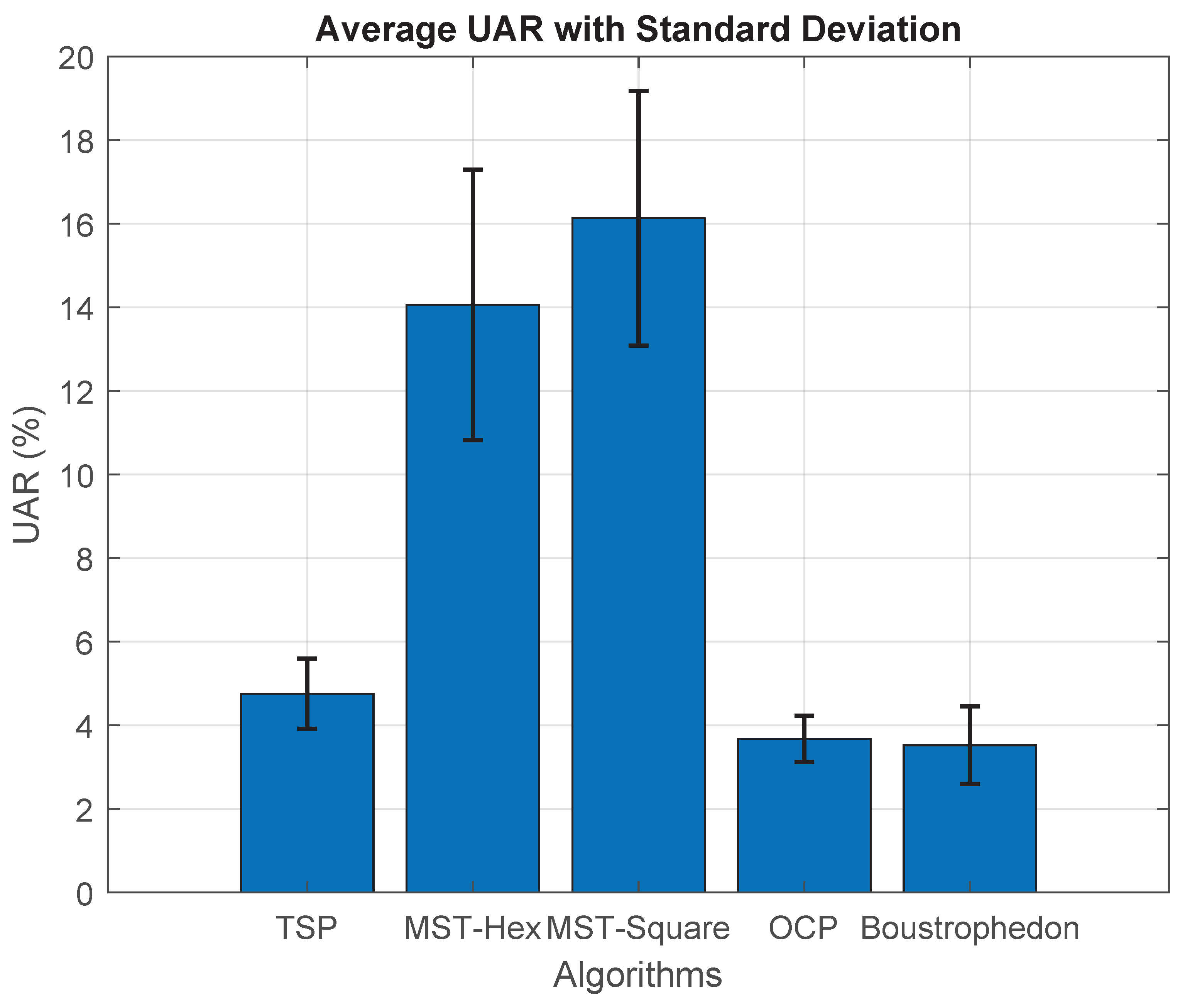
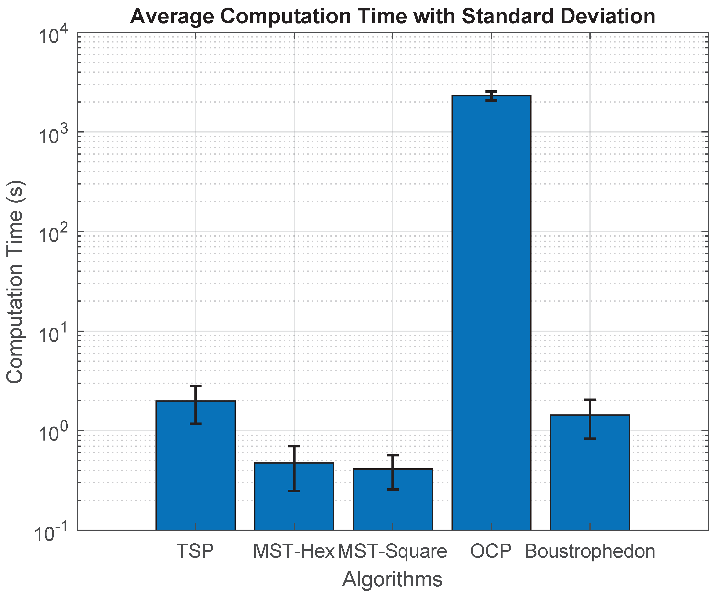
4.2. Aggregate Performance over 10 Samples

Table 1 summarizes the average uncovered area ratio (UAR, in %), the average adjusted length of path (ALOP), and the average computation time (in seconds) for each algorithm over 10 distinct maps. The UAR is computed as the percentage of total area left uncovered, while the ALOP is calculated as
( path length ) × ( detection radius ) covered area .
The detection radius is assumed constant across algorithms.
Figure 12, Figure 13 and Figure 14 visualize these comparisons with vertical lines indicating standard deviations.

4.3. Discussion

Table 1 and Figure 12, Figure 13 and Figure 14 allow a direct, quantitative comparison of the five planners in terms of (i) uncovered-area ratio (UAR), (ii) adjusted length-of-path (ALOP), and (iii) wall-clock computation time. All figures quoted below are averages over the ten Monte Carlo maps and their standard deviations.
The Optimal Control Problem (OCP) leaves only 3.67% of the workspace uncovered; it is marginally outperformed by the boustrophedon sweep by about 0.2% points and improves upon the Traveling Salesman Problem (TSP) by 1.1% points. Both minimum-spanning-tree variants (MST-square and MST-hex) are markedly less thorough, missing more than 14% of the domain, i.e., roughly four times the uncovered area of the OCP. Switching from a square to a hexagonal tiling consistently reduces this deficit by about two percentage points, and the associated confidence bands do not overlap with those of the two near-optimal methods, confirming that the gap is systematic rather than map-specific.
The boustrophedon sweep is the clear outlier with an ALOP of 18.35 , which is approximately 14% longer than the TSP trajectory and 19% longer than the OCP. Its alternating stripes generate excessive overlap and retracing, so that the modest gain in runtime cannot compensate for the long track. MST-square records the numerically smallest ALOP ( 14.54 ) but only because it simply skips large portions of the workspace; once the path length is normalized by the actually covered area, the OCP and MST-hex occupy a narrow band between 14.9 and 15.1 , signalling that the hexagonal tree enjoys essentially the same path efficiency as the globally optimal trajectory.
Solving the nonlinear Optimal Control Problem requires on average 2.3 × 10 3   s on a laptop-class CPU, which is three orders of magnitude slower than any graph-based heuristic. The TSP formulation closes in around two seconds, whereas both MST variants finish in well under half a second, thus meeting hard real-time constraints for on-board replanning. Although the boustrophedon sweep terminates in a respectable 1.4   s , its disadvantage in path length renders it an unattractive compromise.
If near-perfect coverage (UAR below 5%) is critical, the OCP is the method of choice for off-line pre-computation, while the TSP planner provides a viable on-board alternative that sacrifices only about one percentage point of coverage yet is a thousand times faster. When strict real-time operation on a low-power processor is mandatory, the MST-hex heuristic offers the best balance, solving in well under a second while maintaining an uncovered area below 15%. Conversely, if the shortest possible track is the overriding concern and a moderate coverage loss is acceptable, MST-square achieves the lowest path length, whereas the OCP remains the global optimum when no coverage may be sacrificed.

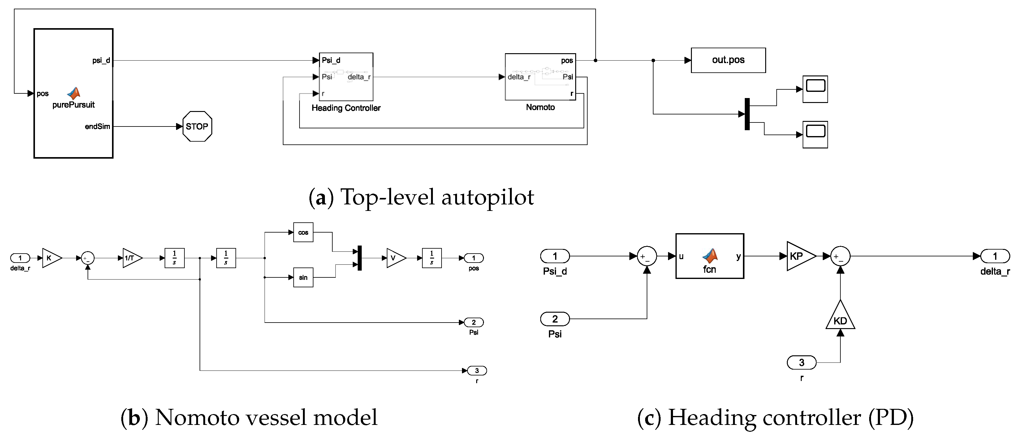
4.4. Marine Application

As a preliminary approach, underwater autonomous gliders will be approximated to an Unmanned Surface Vehicle (USV), which is extensively studied in the literature. For this research, it has been decided to follow the method studied in [3], which is devoted to Mine Countermeasures (MCMs) search missions.
An underwater autonomous glider is approximated to an Unmanned Surface Vehicle (USV), which conducts search missions at a constant velocity and therefore exhibits simple planar motion at the sea surface (pitch, roll, and heave motions are zero). For the sake of simplicity, some assumptions were considered as follows:
  • Zero stream current.
  • Vehicle traveling at a constant speed.
  • The problem is considered to be a simple planar motion at the sea surface (i.e., pitch, roll, and heave motions are zero).
  • Yaw rate can be directly controlled. (The Nomoto time constant is considered to be very large)
Assuming also that no sway slipping is present, the equations of motion (EOM) can be easily modeled by kinematics as in Equations (28) to (31).
Let the state variable pair ( x ( t ) , y ( t ) ) be the vehicle’s position (vertical and horizontal respectively) in meters north and east from an inertial reference frame, ψ ( t ) be its heading angle in radians measured clockwise from north, and r ( t ) be its turn rate in radians per second. If the vehicle travels at constant forward velocity V meters per second, the state-space Equation of Motion (EOM) for the state vector x ( t ) [ x ( t ) , y ( t ) , ψ ( t ) , r ( t ) ] T and control input δ r ( t ) , corresponding to the commanded rudder deflection, are
x ˙ ( t ) = V c o s ψ ( t ) ,
y ˙ ( t ) = V s i n ψ ( t ) ,
ψ ˙ ( t ) = r ( t ) ,
r ˙ ( t ) = 1 T ( K δ r ( t ) r ( t ) ) .
Equation (31) implements a first-order approximation to the well-known Nomoto model for ship-steering equations. In this paper, we consider the model of a SeaFox USV described in Table 2.
The commanded rudder deflection δ r is generated by a proportional–derivative (PD) law acting on the wrapped heading error. First, the raw error ψ d ψ is folded onto the principal interval ( π , π ] through
ψ ˜ = Wrap ψ d ψ , Wrap ( x ) = ( x + π ) mod 2 π π ,
so that the controller never commands a rotation larger than π . The PD term then reads
δ r = K P ψ ˜ K D r
In the sequel, K P = 1.2 and K D = 3.0 were found to yield a satisfactory response.
Way-points w 0 , , w N R 2 define a poly-line to be tracked. Let p = [ x , y ] be the current vehicle position and L d the look-ahead distance.
(a)
Segment selection. Starting from the last active index k, advance to the first segment w k w k + 1 whose end-point w k + 1 is still at least L d ahead of p .
(b)
Orthogonal projection. With d = w k + 1 w k and L s = d , compute
s = clip ( p w k ) d L s , 0 , L s , p proj = w k + s L s d .
(c)
Carrot point and desired heading. The look-ahead (“carrot”) point is p look = p proj + L d L s d . Bearing to that point defines the desired heading
ψ d = atan 2 y look y , x look x
where atan 2 ( · , · ) is the four-quadrant arctangent. The algorithm terminates when k = N or p w N < L d , in which case ψ d simply points to the final way-point. In this paper, we consider the value L d = 20 m
Equations (32)–(34), together with the Nomoto dynamics in (28)–(31), fully specify the closed-loop system, implemented in Simulink, illustrated in Figure 15.
Figure 16, Figure 17, Figure 18, Figure 19 and Figure 20 plot the closed-loop trajectories for each planner on the same test map. The heading controller keeps the vessel closely aligned with every reference path, although small off-track excursions, typically well below the sensor footprint, can still be observed. To guarantee clearance in the presence of these tracking errors, static obstacles should be inflated during the path-generation phase, adding a safety margin equal to the expected maximum deviation. The test map covers a rectangular region roughly 1200 m in length and 900 m in height. The detection radius of the sensor is considered to be 125 m. All simulated runs consider a SeaFox USV whose hull length is 1.2 m.

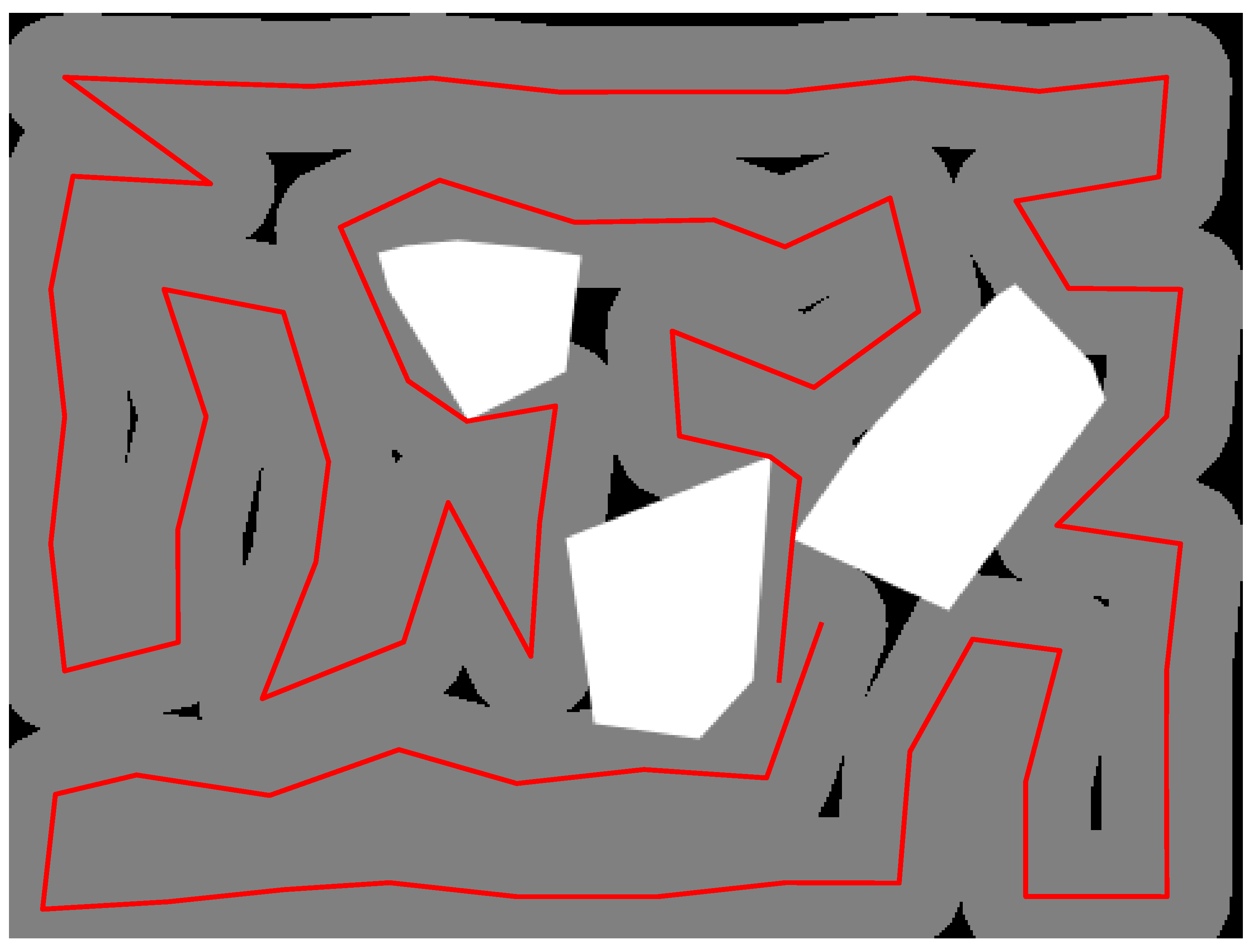
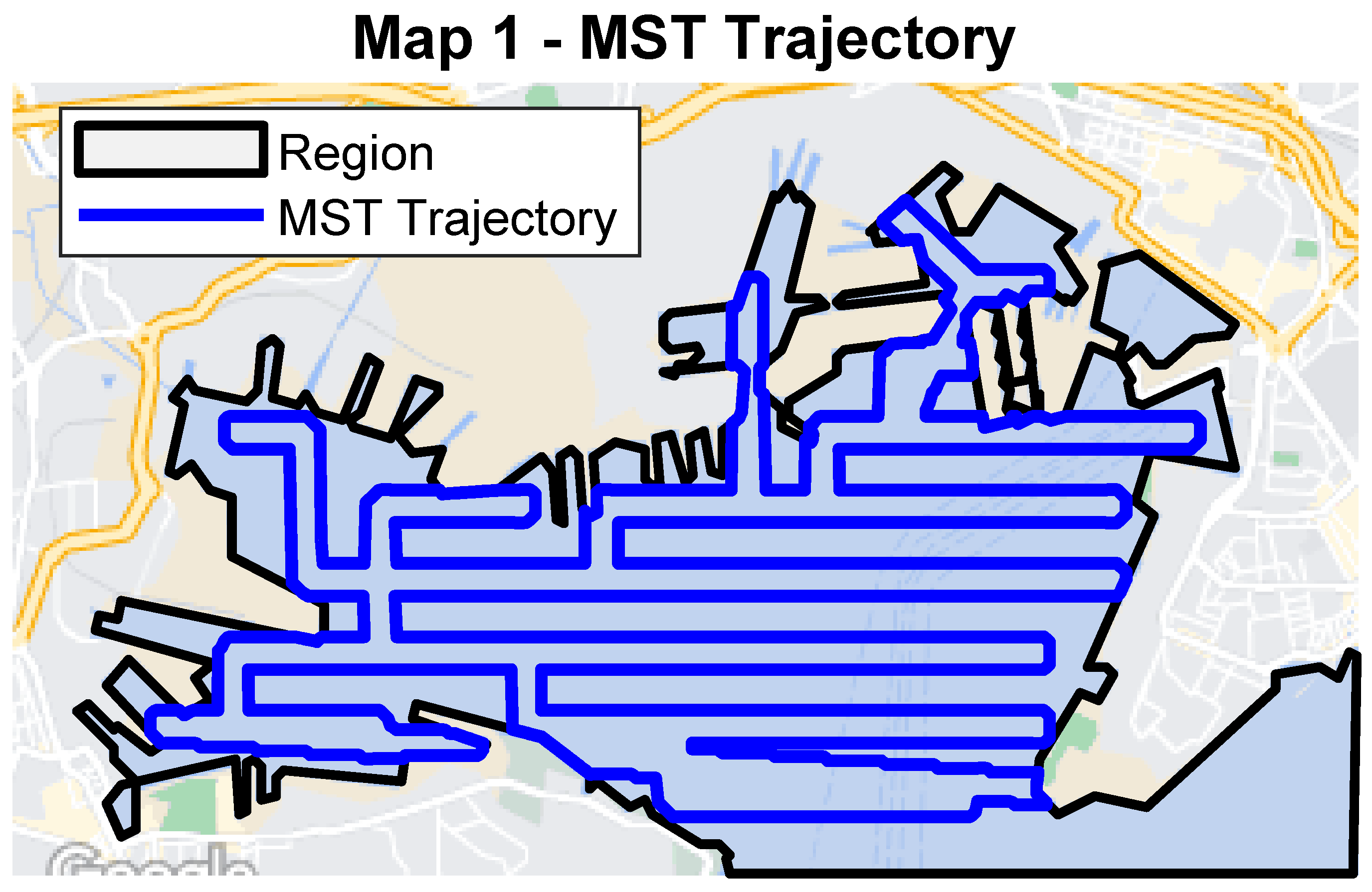
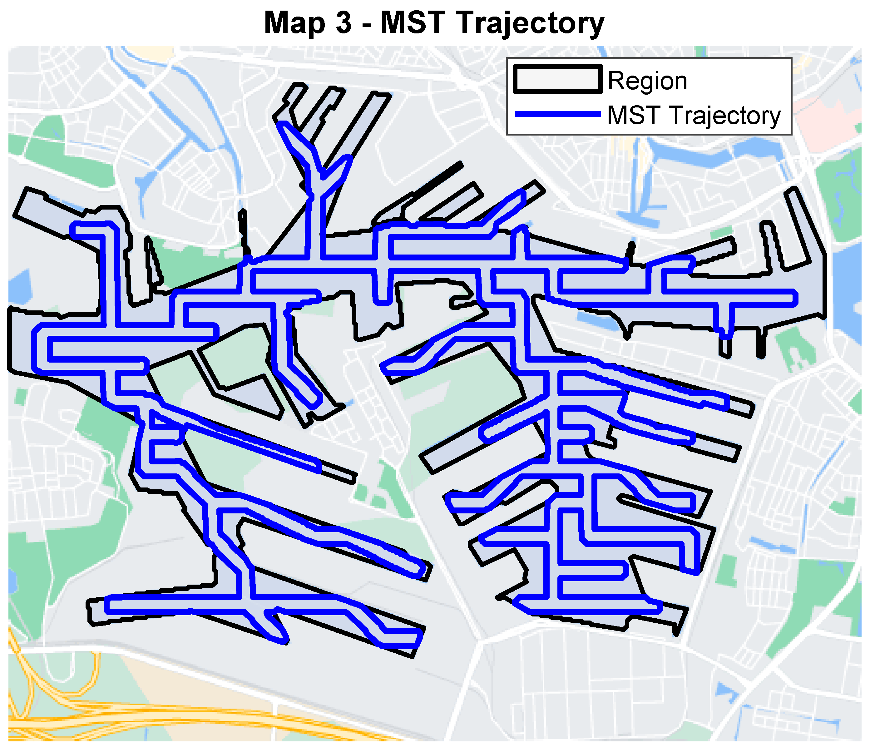
4.5. Outer Polygon Extraction from Map Images

Our approach automatically extracts an outer boundary polygon from map images to define the region of interest for coverage path planning. The segmentation process, based on color thresholding and subsequent contour extraction, produces a clean boundary delineating the area to be covered. This outer polygon is then used to compute a coverage path via an MST-based method, which scales efficiently and is therefore preferred over alternative approaches with higher computational costs.
Figure 21 shows the result for the Toulon map, Figure 22 for the Sines map, and Figure 23 for the Rotterdam map. In all cases, the original map image is presented in the background; the extracted outer polygon is overlaid as a semi-transparent contour, and the corresponding MST-based trajectory is superimposed in blue.
These results confirm that our framework reliably extracts the region’s outer boundary from various map images, enabling efficient coverage path planning using the MST-based method.

5. Conclusions

Trajectory generation is a crucial problem in the context of autonomous vehicle operations particularly when extensive area coverage and efficient traversal are required. Coverage algorithms are designed to generate trajectories that maximize the probability of detecting specific targets while ensuring comprehensive coverage of the environment. This is often formulated as a generalized Optimal Control Problem (OCP) with an appropriate detection model.
To enable a fair comparison with alternative approaches found in the literature, the Traveling Salesman Problem (TSP) and Minimum Spanning Tree (MST) algorithms were implemented. These methods were evaluated against the OCP-based approach based on key performance criteria such as processing time, uncovered areas, and the total distance and duration of the generated trajectory. The results indicate that the OCP is particularly useful when traversal time is constrained; however, it requires significantly higher processing time than alternative methods. Conversely, when maximizing coverage is the primary objective, TSP-based approaches perform better. Additionally, if a rapid solution is required, MST-based approaches yield lower computational costs.

Future Work

Applying a Voronoi-based coverage path-planning approach could also yield promising results. Huang et al. [16] propose a method for path planning in irregular environments, such as those encountered in autonomous mowing applications. Their approach leverages Voronoi diagrams to segment the environment into distinct regions, allowing for systematic coverage while avoiding obstacles. Adopting a similar strategy in the context of vehicle navigation could enhance coverage efficiency and adaptability to complex terrains.

Author Contributions

Conceptualization, F.F.C.R. and É.B.; methodology, A.I., F.F.C.R. and É.B.; software, A.I., F.F.C.R. and É.B.; investigation, A.I., F.F.C.R. and É.B.; writing—original draft preparation, A.I., F.F.C.R. and É.B.; writing—review and editing, A.I., F.F.C.R. and É.B.; All authors have read and agreed to the published version of the manuscript.

Funding

This work was supported by European Commission via Erasmus Mundus Joint Masters Degrees (EMJMD) “Marine and Maritime intelligent robotics” and Fundação para a Ciência e Tecnologia under the projects UIDB/04111/2020 and CTS/00066.

Data Availability Statement

The original data presented in the study are openly available in GitHub at https://github.com/ffcrego87/cover_planning (accessed on 17 June 2025).

Acknowledgments

This work was inspired by the pioneering research of Isaac Kaminer and António Pascoal, which guided the development of the optimal-control approach adopted herein.

Conflicts of Interest

The authors declare no conflicts of interest.

References

  1. Koopman, B.O. The Theory of Search. II. Target Detection. Oper. Res. 1956, 4, 503–531. [Google Scholar] [CrossRef]
  2. Chudnovsky, D.V.; Chudnovsky, G.V. Search Theory: Some Recent Developments; CRC Press: Boca Raton, FL, USA, 2023. [Google Scholar]
  3. Kragelund, S.; Walton, C.; Kaminer, I.; Dobrokhodov, V. Generalized Optimal Control for Autonomous Mine Countermeasures Missions. IEEE J. Ocean. Eng. 2021, 46, 466–496. [Google Scholar] [CrossRef]
  4. Chung, T.H.; Hollinger, G.A.; Isler, V. Search and pursuit-evasion in mobile robotics: A survey. Auton. Robot. 2011, 31, 299–316. [Google Scholar] [CrossRef]
  5. Karaman, S.; Frazzoli, E. Sampling-based algorithms for optimal motion planning. Int. J. Robot. Res. 2011, 30, 846–894. [Google Scholar] [CrossRef]
  6. Masakuna, J.F.; Utete, S.W.; Kroon, S. A Coordinated Search Strategy for Solitary Robots. In Proceedings of the 2019 Third IEEE International Conference on Robotic Computing (IRC), Naples, Italy, 25–27 February 2019; IEEE: New York, NY, USA, 2019; pp. 433–434. [Google Scholar]
  7. Ismail, Z.; Hamami, M. Systematic literature review of swarm robotics strategies applied to target search problem with environment constraints. Appl. Sci. 2021, 11, 2383. [Google Scholar] [CrossRef]
  8. Yang, J.; Wang, X.; Bauer, P. Extended pso based collaborative searching for robotic swarms with practical constraints. IEEE Access 2019, 7, 76328–76341. [Google Scholar] [CrossRef]
  9. Luo, Y.; Ye, G.; Wang, Y.; Xie, L.; Wang, X.; Zhang, S.; Yan, X. Toward target search approach of swarm robotics in limited communication environment based on robot chains with elimination mechanism. Int. J. Adv. Robot. Syst. 2020, 17, 172988142091995. [Google Scholar] [CrossRef]
  10. Zhou, Y.; Chen, A.; He, X.; Bian, X. Multi-target coordinated search algorithm for swarm robotics considering practical constraints. Front. Neurorobot. 2021, 15, 753052. [Google Scholar] [CrossRef] [PubMed]
  11. Batalin, M.; Sukhatme, G. Coverage, exploration and deployment by a mobile robot and communication network. Telecommun. Syst. 2004, 26, 181–196. [Google Scholar] [CrossRef]
  12. Galceran, E.; Carreras, M. A survey on coverage path planning for robotics. Robot. Auton. Syst. 2013, 61, 1258–1276. [Google Scholar] [CrossRef]
  13. Le, A.; Veerajagadheswar, P.; Sivanantham, V.; Mohan, R. Modified a-star algorithm for efficient coverage path planning in Tetris inspired self-reconfigurable robot with integrated laser sensor. Sensors 2018, 18, 2585. [Google Scholar] [CrossRef] [PubMed]
  14. Strimel, G.P.; Veloso, M.M. Coverage planning with finite resources. In Proceedings of the 2014 IEEE/RSJ International Conference on Intelligent Robots and Systems, Chicago, IL, USA, 14–18 September 2014; IEEE: New York, NY, USA, 2014; pp. 2950–2956. [Google Scholar]
  15. Khan, A.; Noreen, I.; Ryu, H.; Doh, N.L.; Habib, Z. Online complete coverage path planning using two-way proximity search. Intell. Serv. Robot. 2017, 10, 229–240. [Google Scholar] [CrossRef]
  16. Huang, K.C.; Lian, F.L.; Chen, C.T.; Wu, C.H.; Chen, C.C. A novel solution with rapid Voronoi-based coverage path planning in irregular environment for robotic mowing systems. Int. J. Intell. Robot. Appl. 2021, 5, 558–575. [Google Scholar] [CrossRef]
  17. Höffmann, M.; Patel, S.; Büskens, C. Optimal coverage path planning for agricultural vehicles with curvature constraints. Agriculture 2023, 13, 2112. [Google Scholar] [CrossRef]
  18. Jayalakshmi, K.; Nair, V.G.; Sathish, D.; Guruprasad, K. Adaptive Spanning Tree based Coverage Path Planning for Autonomous Mobile Robots in Dynamic Environments. IEEE Access 2025, 13, 102931–102950. [Google Scholar] [CrossRef]
  19. Hung, N.T.; Rego, F.; Crasta, N.; Pascoal, A.M. Input-constrained path following for autonomous marine vehicles with a global region of attraction. IFAC-PapersOnLine 2018, 51, 348–353. [Google Scholar] [CrossRef]
  20. Gkesoulis, A.K.; Georgakis, P.; Karras, G.C.; Bechlioulis, C.P. Autonomous Sea Floor Coverage with Constrained Input Autonomous Underwater Vehicles: Integrated Path Planning and Control. Sensors 2025, 25, 1023. [Google Scholar] [CrossRef] [PubMed]
  21. Rego, F.; Hung, N.; Pascoal, A. Cooperative path-following of autonomous marine vehicles: Theory and experiments. In Proceedings of the 2018 IEEE/OES Autonomous Underwater Vehicle Workshop (AUV), Porto, Portugal, 6–9 November 2018; IEEE: New York, NY, USA, 2018; pp. 1–6. [Google Scholar]
  22. Graham, R.; Hell, P. On the History of the Minimum Spanning Tree Problem. Ann. Hist. Comput. 1985, 7, 43–57. [Google Scholar] [CrossRef]
  23. Gabriely, Y.; Rimon, E. Spanning-tree based coverage of continuous areas by a mobile robot. Ann. Math. Artif. Intell. 2001, 31, 77–98. [Google Scholar] [CrossRef]
  24. Hazon, N.; Kaminka, G.A. Redundancy, efficiency and robustness in multi-robot coverage. In Proceedings of the 2005 IEEE International Conference on Robotics and Automation, Barcelona, Spain, 18–22 April 2005; IEEE: New York, NY, USA, 2005; pp. 735–741. [Google Scholar]
  25. Merci, A.; Anthierens, C.; Thirion-Moreau, N.; Le Page, Y. Management of a fleet of autonomous underwater gliders for area coverage: From simulation to real-life experimentation. Robot. Auton. Syst. 2025, 183, 104825. [Google Scholar] [CrossRef]
  26. Li, Y.; Gu, N.; Jia, J.; Peng, Z.; Wang, D. Simulated Annealing-Based Optimization for the Coverage Path Planning of Multiple Unmanned Surface Vehicles in ECDIS. In Proceedings of the 2024 14th International Conference on Information Science and Technology (ICIST), Chengdu, China, 6–9 December 2024; IEEE: New York, NY, USA, 2024; pp. 188–193. [Google Scholar]
  27. Laporte, G. The traveling salesman problem: An overview of exact and approximate algorithms. Eur. J. Oper. Res. 1992, 59, 231–247. [Google Scholar] [CrossRef]
  28. Walton, C.L.; Gong, Q.; Kaminer, I.; Royset, J.O. Optimal Motion Planning for Searching for Uncertain Targets. Ifac Proc. Vol. 2014, 47, 8977–8982. [Google Scholar] [CrossRef]
  29. Andersson, J.A.E.; Gillis, J.; Horn, G.; Rawlings, J.B.; Diehl, M. CasADi—A software framework for nonlinear optimization and optimal control. Math. Program. Comput. 2019, 11, 1–36. [Google Scholar] [CrossRef]
  30. Lin, S. Computer solutions of the traveling salesman problem. Bell Syst. Tech. J. 1965, 44, 2245–2269. [Google Scholar] [CrossRef]
  31. Rego, F.F.C. Cover_Planning: Coverage Planning Algorithms for Underwater Robotics. 2025. Available online: https://github.com/ffcrego87/cover_planning (accessed on 17 June 2025).
Figure 1. Main principle for the covering.
Jmse 13 01369 g001
Figure 2. Construction of trajectory: we create a 2r-grid (a) we compute a minimal spanning tree (b) we perform a dilatation of this spanning tree of radius r (c) and we finally obtain a trajectory as the border of the dilated tree (d).
Jmse 13 01369 g002
Figure 3. Square grid.
Jmse 13 01369 g003
Figure 4. Algorithm.
Jmse 13 01369 g004
Figure 5. Construction of the path.
Jmse 13 01369 g005
Figure 6. Same algorithm with Euclidian distance.
Jmse 13 01369 g006
Figure 7. Representative trajectory: MST-squared path on a single map.
Jmse 13 01369 g007
Figure 8. Representative trajectory: MST-hex path on a single map.
Jmse 13 01369 g008
Figure 9. Representative trajectory: TSP path on a single map.
Jmse 13 01369 g009
Figure 10. Representative trajectory: OCP path on a single map.
Jmse 13 01369 g010
Figure 11. Representative trajectory: boustrophedon path on a single map.
Jmse 13 01369 g011
Figure 12. Average UAR (%) with standard deviation for each algorithm.
Jmse 13 01369 g012
Figure 13. Average ALOP with standard deviation for each algorithm.
Jmse 13 01369 g013
Figure 14. Average computation time (log scale) with standard deviation for each algorithm.
Jmse 13 01369 g014
Figure 15. Simulink implementation of the guidance-control loop used for the marine case study. The three cascaded subsystems realize (a) path following via a pure-pursuit algorithm, (b) heading control through a PD law with yaw-rate feedback, and (c) first-order vessel dynamics given by the Nomoto model.
Jmse 13 01369 g015
Figure 16. Closed-loop trajectory for the MST–square planner.
Jmse 13 01369 g016
Figure 17. Closed-loop trajectory for the MST–hex planner.
Jmse 13 01369 g017
Figure 18. Closed-loop trajectory for the TSP planner.
Jmse 13 01369 g018
Figure 19. Closed-loop trajectory for the OCP planner.
Jmse 13 01369 g019
Figure 20. Closed-loop trajectory for the Boustrophedon planner.
Jmse 13 01369 g020
Figure 21. The Toulon map, with its extracted outer boundary, and the computed MST-based coverage trajectory overlaid on the original image.
Jmse 13 01369 g021
Figure 22. The Sines map showing the extracted boundary and the MST-based trajectory, demonstrating effective area coverage.
Jmse 13 01369 g022
Figure 23. The Rotterdam map with the outer polygon and MST-based coverage path, ensuring all areas within the boundary are visited.
Jmse 13 01369 g023
Table 1. Aggregated results over 10 samples. The order is TSP, MST-hex, MST-square, OCP, Boustrophedon.
AlgorithmAvg. UAR (%)Avg. ALOPAvg. Time (s)
TSP4.7615.80 1.99
MST-hex14.0615.14 0.47
MST-square16.1314.54 0.41
OCP3.6714.922306
Boustrophedon3.5218.35 1.44
Table 2. Design parameters for a SeaFox USV model.
Design ParameterValue
Nomoto Gain Constant, K0.5 1/s
Nomoto Time Constant, T5.0 s
Velocity, V2.5 m/s
Disclaimer/Publisher’s Note: The statements, opinions and data contained in all publications are solely those of the individual author(s) and contributor(s) and not of MDPI and/or the editor(s). MDPI and/or the editor(s) disclaim responsibility for any injury to people or property resulting from any ideas, methods, instructions or products referred to in the content.

