Vision-Based Underwater Docking Guidance and Positioning: Enhancing Detection with YOLO-D

Abstract

This study proposed a vision-based underwater vertical docking guidance and positioning method to address docking control challenges for human-operated vehicles (HOVs) and unmanned underwater vehicles (UUVs) under complex underwater visual conditions. A cascaded detection and positioning strategy incorporating fused active and passive markers enabled real-time detection of the relative position and pose between the UUV and docking station (DS). A novel deep learning-based network model, YOLO-D, was developed to detect docking markers in real time. YOLO-D employed the Adaptive Kernel Convolution Module (AKConv) to dynamically adjust the sample shapes and sizes and optimize the target feature detection across various scales and regions. It integrated the Context Aggregation Network (CONTAINER) to enhance small-target detection and overall image accuracy, while the bidirectional feature pyramid network (BiFPN) facilitated effective cross-scale feature fusion, improving detection precision for multi-scale and fuzzy targets. In addition, an underwater docking positioning algorithm leveraging multiple markers was implemented. Tests on an underwater docking markers dataset demonstrated that YOLO-D achieved a detection accuracy of mAP@0.5 to 94.5%, surpassing the baseline YOLOv11n with improvements of 1.5% in precision, 5% in recall, and 4.2% in mAP@0.5. Pool experiments verified the feasibility of the method, achieving a 90% success rate for single-attempt docking and recovery. The proposed approach offered an accurate and efficient solution for underwater docking guidance and target detection, which is of great significance for improving the safety of docking.

1. Introduction

Deep-sea unmanned underwater vehicles (UUVs) frequently dock and recover from human-occupied vehicles (HOVs) during exploration operations to supplement power, upload data, and download commands, thereby ensuring continuous, efficient, and uninterrupted underwater activities. Visual guidance plays a crucial role in the final stage of the docking process, in which the accuracy and stability of detecting and positioning underwater docking markers are critical for ensuring docking success and safety. However, underwater target detection poses unique challenges compared with standard computer vision tasks owing to complex visual conditions, including inadequate lighting, color distortion, blur, low contrast, and disturbances from water scattering and refraction. These challenges are compounded by the limited computing power and energy resources available on mobile platforms.

Visual-based underwater target detection methods are broadly categorized into traditional methods and deep learning-based approaches [1]. Traditional methods primarily rely on feature extraction and image processing techniques, such as threshold segmentation, edge detection, shape matching, and optical flow, to detect and localize targets. These methods are generally suitable for relatively simple scenarios. For instance, Xu et al. explored underwater visual navigation using multiple ArUco markers and proposed a noise model for single-marker pose estimation and an optimization algorithm for multi-marker pose estimation to improve detection accuracy [2]. However, reliance on manually configured artificial structures makes these methods unsuitable for underwater docking environments. Similarly, Yan et al. proposed a visual positioning algorithm based on an L-shaped light array and demonstrated its feasibility and reliability through docking experiments with AUV recovery [3]. Nevertheless, this approach relies on conventional image detection to locate the light source, and simple positioning techniques demonstrate limited adaptability to dynamic environments and low fault tolerance in the presence of interference. Wang et al. introduced a pseudo-3D visual inertia-based method for AUV localization in a three-dimensional space, incorporating depth information into 2D visual images for robust localization in dynamic underwater conditions [4]. However, this approach requires the fusion of inertial measurement unit data and camera observations, which requires advanced hardware. Lv et al. developed an adaptive binary threshold calculation method for navigation images based on the bright blue point source characteristics of navigation lights, along with an image enhancement approach to reduce navigation feature extraction failures [5]. Finally, Trslić et al. proposed a solution using four conventional light beacons on an umbilical cable management system (TMS), which employs standard image processing algorithms to determine the center of the circle and calculate the relative position and heading [6].

Conventional techniques exhibit a significant vulnerability to environmental factors, especially in intricate underwater environments marked by murky water, inconsistent illumination, disturbances, and various obstacles, all of which frequently compromise detection precision. Although these methods are relatively rapid, they are poorly adapted to dynamic environments, prone to interference, lack robustness, and exhibit low accuracy in target detection. Such shortcomings render them unsuitable for docking control, which demands rapid response and high precision. Consequently, these limitations significantly undermine the practicality and reliability of conventional underwater object detection techniques in docking scenarios.

Compared with conventional object detection methods, deep learning-based approaches are faster, more adaptable, and more resilient in complex scenarios, such as when objects are partially obscured. The You Only Look Once (YOLO) series of object detection models is highly regarded for its exceptional efficiency and real-time capabilities, rendering it especially attractive for applications in underwater object detection. Although the YOLO algorithm has demonstrated superior speed and accuracy across various applications, there remains a need for further enhancement and optimization of its performance to effectively tackle the specific challenges presented by underwater environments. Enhancing the effectiveness and robustness of the YOLO algorithm, particularly for detecting small underwater targets, is crucial under extreme underwater conditions.

Pan et al. presented the YOLOv9s-UI detection model, which enhances feature extraction capabilities by incorporating the Dual Dynamic Token Mixer (D-Mixer) module derived from TransXNet. Additionally, this model integrates the feature fusion network architecture of the LocalMamba network, employing both channel and spatial attention mechanisms [7]. Despite the model’s noteworthy performance on the URPC2019 dataset, its advanced modules present considerable deployment challenges due to their complexity. Specifically, the model’s generalizability and performance in diverse underwater environments require validation using a more extensive range of datasets. Similarly, Liu et al. proposed a novel detection neural network, TC-YOLO, that integrates the Transformer self-attention mechanism, coordinated attention mechanism, image enhancement technique using an adaptive histogram equalization algorithm, and an optimal transmission label assignment scheme [8]. However, combining the training of image enhancement and feature extraction components significantly increases computational demands and resource consumption. Wang et al. augmented the feature extraction component of YOLOv7 by developing an improved image processing branch. This included an underwater image enhancement module followed by a context transfer module, which extracts the domain-specific features from the enhanced image and fuses them with the features from the original image before inputting them into the detector [9]. However, the inferential speed of the model poses challenges when processing complex video data, necessitating further optimization of model size and parameter calculations. Wang et al. also proposed a fast and compact underwater lightweight object detector (ULO) requiring less than 7% of YOLOv3’s computational cost while achieving comparable results [10]. Nevertheless, the experimental results indicated that its performance is only 97.9% of that of the YOLOv3 baseline. Similarly, Chen et al. introduced a lightweight and efficient underwater detection algorithm, YOLO_GN, featuring a novel GhostNetV2-based backbone and integrating Ghost_BottleneckV2 with dynamically sparse attention BiFormer to reduce computational costs and improve accuracy [11]. However, this method struggles to detect complex targets, particularly those in motion or moving rapidly. Zhang et al. proposed a lightweight underwater detection method combining MobileNetv2, the YOLOv4 algorithm, and attention feature fusion [12]. Despite its advancements, this approach still faces limitations in detecting small targets with extreme scale variations.

Deep learning-based YOLO object detection methods can effectively detect objects in dynamic environments. However, they are limited to providing rectangular bounding boxes and cannot detect precise boundary information or accurately estimate position and attitude, making them unsuitable for underwater docking guidance. To address these limitations, Chen et al. proposed a three-dimensional perception algorithm based on the YOLO framework for the precise detection and localization of targets in Underwater Vehicle Manipulator Systems (UVMSs) [13]. Although this approach improves the execution speed by 15% compared to YOLOv8s, it incurs a significant computational burden owing to the integration of binocular stereo vision matching. Similarly, Li et al. developed a visual-based underwater target detection and localization method [14] consisting of a YOLO-T algorithm for detection and a target localization algorithm. This method employs an identification mark composed of four basic dots. Despite its simplicity, it lacks robustness under stress in dynamic environments. The real-time detection and positioning of underwater marks remains unachieved. Liu et al. proposed a generative adversarial network (Tank-to-field GAN, T2FGAN) to model underwater images for data augmentation, aiming to improve detection accuracy [15]. However, the study did not report the detection time, and the GAN network model may exhibit a slower image detection rate. Lwin et al. utilized a real-time multistep genetic algorithm (RM-GA) for vehicle attitude recognition from dynamic images captured by dual cameras, demonstrating robust stereo vision-based real-time position and orientation tracking [16]. Nonetheless, the complex configuration of this binocular visual positioning algorithm can limit its applicability to resource-constrained environments. Sun et al. developed a two-stage docking algorithm using convolutional neural networks (CNNs) to estimate the three-dimensional relative positions and orientations of DS and AUVs, incorporating phase detection and pose estimation via the Perspective-n-Point (PnP) method [17]. However, the two-stage recognition approach can reduce the identification efficiency of guide light sources. Liu et al. introduced a Laplacian-of-Gaussian-based coarse-to-fine blockwise (LCB) landmark detection method and a convolutional neural network (DoNN) for bounding box detection and pose estimation [18]. Despite these innovations, the method had a relatively slow detection rate, with an average processing time of 0.17 s per frame.

To the best of our knowledge, there is limited research on leveraging deep learning techniques to effectively address the challenges of landmark detection and localization for autonomous underwater docking guidance. In response to these challenges, this study proposed a novel methodology comprising a docking mark detection algorithm and a target positioning algorithm. These methods significantly improved the precision and reliability of underwater mark detection, thereby enhancing the efficacy and safety of underwater docking and recovery operations.

The principal contributions of this research are outlined as follows.

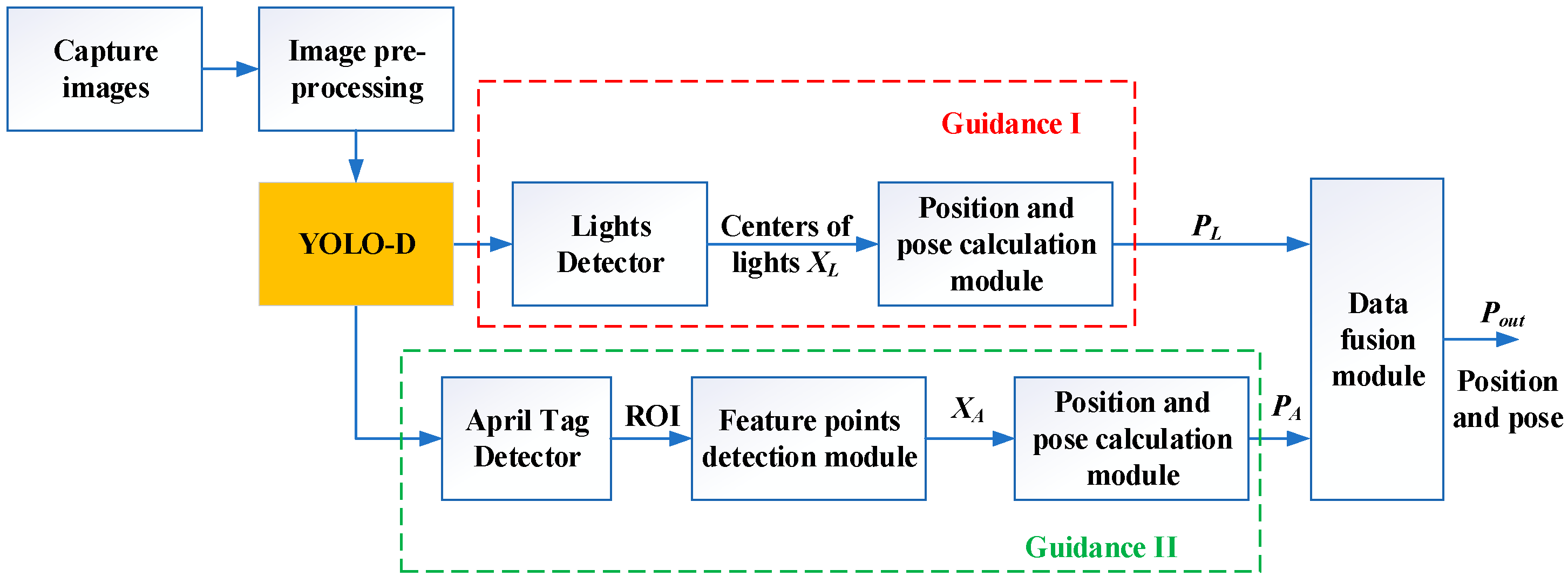
• A novel visual guidance framework was proposed for underwater drop-in docking. It incorporated cascaded detection and a positioning strategy that integrated the active and passive markers. The strategy utilized light arrays for long-distance guidance and AprilTag for close-range positioning, effectively combining the benefits of an extended operational range with high precision.
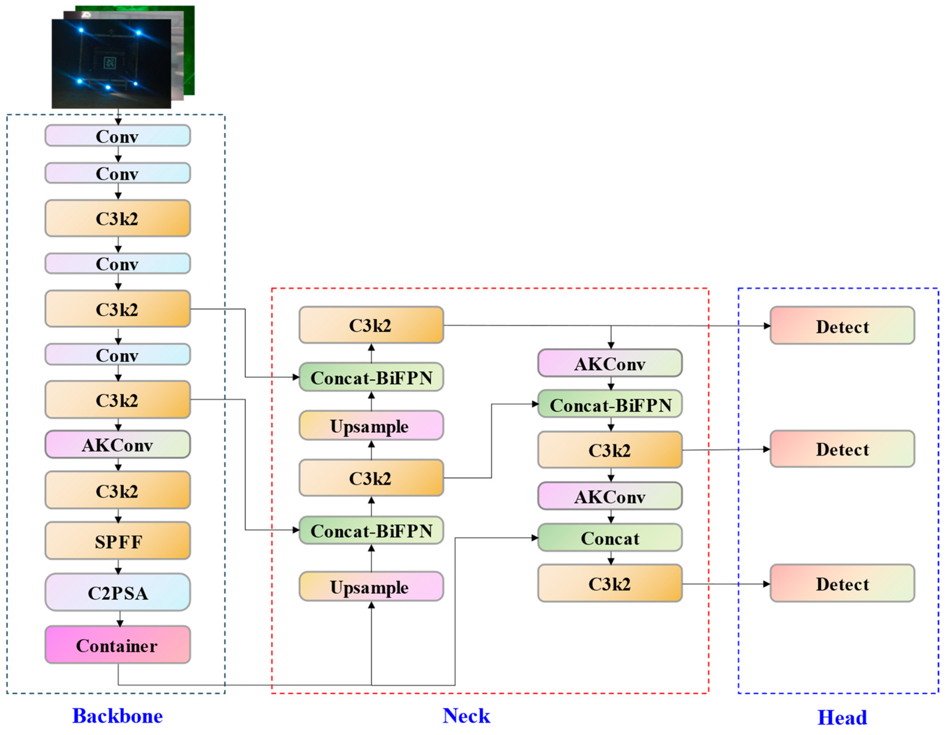
• This study introduced a novel network model, YOLO-D, designed to detect and localize docking marks under complex underwater visual conditions. The model utilized the adaptive convolution kernel, AKConv, which dynamically adjusted its sampling shape and parameter count based on the specific characteristics of the images and targets, thereby enhancing the accuracy and efficiency of feature extraction. To improve the detection of small underwater targets, the CONTAINER mechanism was incorporated for context enhancement and feature refinement. In addition, a BiFPN was integrated to enable efficient multi-scale feature fusion, allowing faster and more effective processing of multi-scale targets at various distances during underwater docking.
• We constructed a dedicated underwater docking marker dataset and conducted camera calibration, comparison, and ablation tests for underwater target detection. In comparison to the baseline model, YOLOv11n, the proposed YOLO-D method demonstrated enhancements of 1.5% in precision, 5% in recall, 4.2% in mAP@0.5, and 3.57% in the F1 score. In addition, a successful underwater landing docking visual guidance pool test was conducted, achieving a 90% recovery success rate. These results validated the feasibility of the proposed docking guidance method.

The remainder of this paper is organized as follows. Section 2 introduces the underwater docking guidance localization framework and algorithm. Section 3 details the design and improvement methods of the YOLO-D docking target detection model and multi-signature localization algorithm. Section 4 presents the underwater docking target dataset, comparative target detection experiments, and ablation experiments and verifies the effectiveness of the proposed method through an underwater docking guidance localization experiment. In conclusion, Section 5 provides a summary of this study and explores possible avenues for future research endeavors.

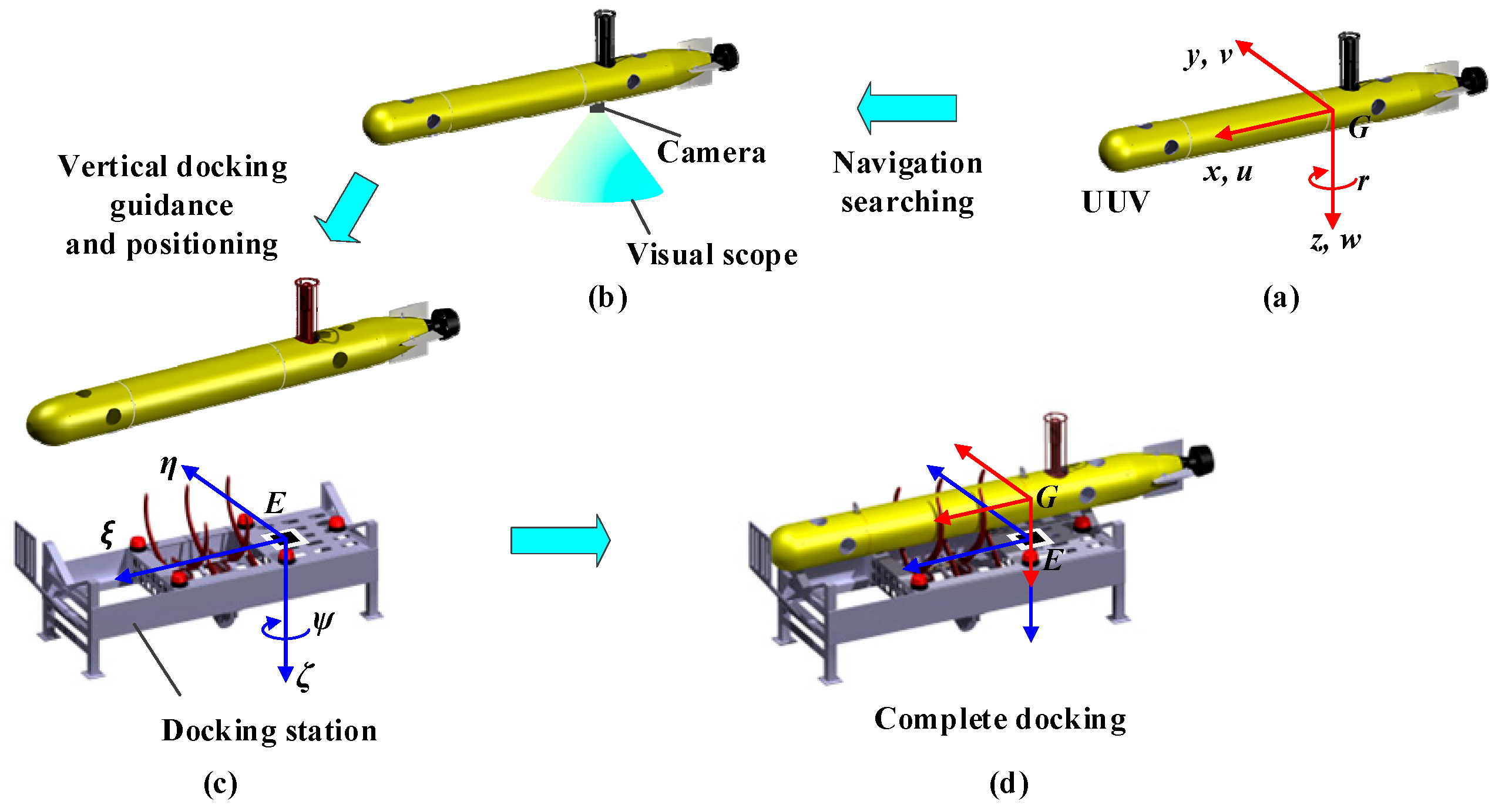
2. Docking Guidance and Positioning Framework

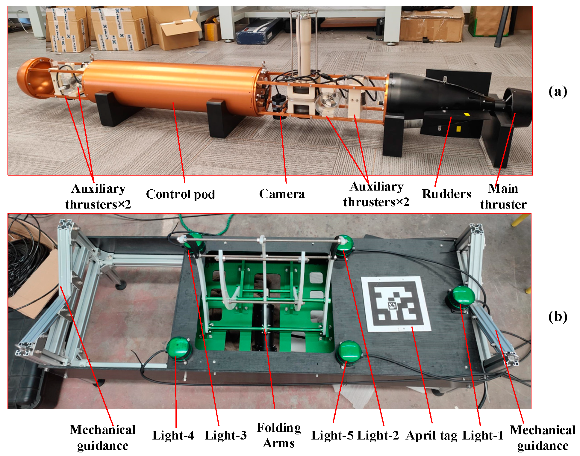
2.1. System Structure of Docking Guiding System

A human-occupied vehicle (HOV) facilitates the docking and retrieval of an unmanned underwater vehicle (UUV) in either a bottom-sitting or underwater hovering state by using a docking station (DS). A schematic diagram and coordinate system of the underwater landing docking principle are shown in Figure 1. In Figure 1a, the reference body frame (RBF) $G-xyz$ was affixed to the UUV, with its origin positioned at the center of gravity $G$ of the UUV. A set of downward-facing underwater cameras was mounted at the center of the UUV to enable visual detection and positioning (Figure 1b). The north-east-down (NED) frame $E-\xi \eta \zeta$ of the geodetic coordinate system was fixed to the DS, with its origin $E$ located at the center point of the DS (Figure 1c).

During the underwater landing docking procedure, the UUV employed an underwater camera to capture real-time images of the DS and its markers. A visual guidance positioning algorithm was employed to compute the relative position and orientation between the UUV and the DS in real time. Simultaneously, the auxiliary and main propulsion systems of the UUV were automatically adjusted to realign its position and attitude during vertical descent. Upon completion of the docking and recovery processes, the states of points G (on the UUV) and E (on the DS) were nearly identical (Figure 1d).

The underwater landing, docking, guidance, and positioning system developed in this study is illustrated in Figure 2. It consisted of two main components: a UUV and a DS. As shown in Figure 2a, a set of downward-facing underwater cameras was mounted at the center of the UUV to capture the images of the underwater docking markers. Two propulsion units positioned at the front and rear of the UUV enabled horizontal and vertical maneuvers. Additionally, a rudder, elevator, and main propulsion device at the rear regulated underwater navigation. Figure 2b depicts a DS featuring five underwater lights and an AprilTag symmetrically arranged along its centerline to serve as a docking marker. V-shaped mechanical guide devices were located at the head and tail of the DS for passive guidance, whereas a retractable mechanical arm at its center provided active guidance and positive locking.

2.2. Docking Guidance Strategies

To ensure the safe and reliable execution of the underwater landing and docking process, machine vision should provide stable, accurate, and efficient guidance and positioning. The most prevalent docking approach is the cage-type mode [19], which typically utilizes a single type of target, such as a light array or two-dimensional code, as a positioning marker. However, this method cannot simultaneously optimize the range and detection accuracy. At long distances, the light array served as a docking marker. However, it fell outside the camera’s field of view at a close range. Consequently, the UUV relied only on its inertia, mechanical guidance, or collision with the cage for docking and recovery. Another method involves the application of specialized markers [20]. Although it can be highly accurate, it can severely limit the effective range for underwater positioning.

Building on insights from the literature, this study proposed an active/passive landmark cascade underwater guidance and positioning strategy. This strategy was designed to determine the 4-DOF pose information $P_{out}={\left[\begin{array}{c}\xi ,\eta ,\zeta ,\psi \end{array}\right]}^T$ of the UUV relative to the DS. The approach employed a two-stage fusion visual positioning method that utilized both active and passive visual landmarks.

• Level I guidance adopted an array of lights as visual markers, offering a considerable visible range owing to their active light emission. However, at closer distances, light scattering introduced certain errors in estimating the center of the guidance light source, making this method suitable only for coarse posture adjustments during docking. In addition, in the final stages of docking, it became difficult to maintain all guidance lights within the field of view of the camera, leading to a high failure rate.
• Level II guidance utilized a specific graphic, AprilTag, as an identification marker, estimating the pose by detecting its characteristic points. This method offered high positioning accuracy. However, its effectiveness was limited by underwater visibility, which is influenced by certain factors such as water quality, turbidity, and illumination. Consequently, it may be suitable for fine adjustments during docking.

As illustrated in Figure 3, the process began with image capture using an underwater camera. The images were then pre-processed through filtering and enhancement to improve the signal-to-noise ratio. The core module YOLO-D based on deep learning was employed to detect the center $X_L$ of the lights and identify the region of interest (ROI) containing AprilTag. In Level I guidance, the center $X_L$ of the lights was applied to calculate $P_L$ using the position and attitude detection module. In Level II guidance, the AprilTag within the ROI was detected, and the coordinates $X_A$ of its four vertices were determined. Subsequently, the position and attitude detection modules were employed to calculate $P_A$. Finally, the data fusion module computed the overall position and attitude $P_{out}$ of the UUV relative to DS, as expressed by the following formula:

$$P_{out}=K_1{P}_L+{K_{2}P}_A,$$

(1)

where $K_1$ and $K_2$ represent the weight matrices utilized for data fusion, which were adjusted according to prevailing circumstances.

Remark 1.

Under optimal water quality conditions, overlapping visual positioning areas may allow for simultaneous positioning using both active and passive markers. Information fusion methods such as extended Kalman filtering can be employed to improve the stability and accuracy of the algorithm. However, disturbances in both Level I and Level II measurements can result in outliers. Therefore, a filtration process is essential to ensure the accuracy and reliability of detection results.

Remark 2.

As the distance changes, the reliability and accuracy of two-level visual positioning also vary. To account for this, the weight matrices $K_1$ and $K_2$ in the output results of the two methods must be adaptively adjusted to enable fusion of the positioning information. Under poor water quality conditions, visual positioning may encounter blind spots or obstructions from interfering objects, making the simultaneous detection of active and passive markers impossible. In such cases, positioning can still be achieved as long as either level remains effective.

2.3. Docking Guidance Algorithms

This study developed a novel approach for underwater landing docking by integrating the advantages of active and passive markers into a cascaded guidance and positioning algorithm (Algorithm 1).

Algorithm 1: Docking Guidance Algorithm

1: Capture images;  2: Perform image pre-processing: Gaussian and median filter are employed;  3: Run the YOLO-D module to detect lights and AprilTag;  4: Calculate the number of lights $N_L$, and the number of AprilTag $N_A$;  5: While $(C_A\le T_A)$ and $(C_L\le T_L)$ do  6:  If $N_L=5$  7:     Obtain the pixel values $X_L$ of the lights from YOLO-D;  8:     Calculate position and pose $P_L$ by RPnP algorithm;  9:     Perform smoothing filtering; 10:    Reset the counter $C_L=0$; 11:  else 12:     Counter Accumulation $C_L=C_L+1$; 13:  end if 14:  If $N_A=1$ 15:     Obtain the pixels of the vertices of the ROI where the AprilTag is located.      from YOLO-D; 16:     Extract the Contours of AprilTag using CANNY Algorithm; 17:     Calculate position and pose $P_A$ from the vertices $X_A$ of AprilTag; 18:     Perform smoothing filtering; 19:     Reset the counter $C_A=0$; 20:  else 21:    Counter Accumulation $C_A=C_A+1$; 22:  end if 23:  Fusion calculate position and pose $P_{out}$ with $P_L$ and $P_A$. 24: end while 25: Docking procedure ends.

Remark 3.

The proposed algorithm may fail to detect valid markers under extreme conditions, rendering the subsequent visual positioning phase infeasible. In such cases, the pose established in the preceding step can be used for docking control to increase the likelihood of capturing valid marker images in the next iteration, by bringing the ROV closer to the dock. If the number of iterations exceeds the safety threshold and the pose remains unestimated, the docking control of the ROV is terminated.

3. Target Detection and Positioning Methods

3.1. YOLOv11

Compared with other models in the series, YOLOv11 offers significant advantages in terms of feature extraction, efficiency, speed, cross-environment adaptability, and versatility across diverse tasks. It incorporates an enhanced backbone network and neck architecture, enabling more precise feature extraction and improved performance in complex tasks. Its refined design and optimized training process can ensure faster processing speeds while maintaining an optimal balance between accuracy and performance. Additionally, YOLOv11 achieved a higher mean average precision (mAP) on the COCO dataset while using 22% fewer parameters than YOLOv8, demonstrating superior computational efficiency without sacrificing accuracy. The complete configuration of the YOLOv11 network is illustrated in Figure 4, highlighting its structure and key innovations [21]. As illustrated in Figure 4, the YOLOv11n baseline model is comprised of 238 layers.

3.2. YOLO-D Network Model

In an underwater docking scenario, water selectively absorbs light of different wavelengths and depths. This is the phenomenon known as the absorption spectrum. Red light with lower energy is absorbed first, causing the underwater images or video data to exhibit a bluish or greenish hue. Furthermore, the scattering of light caused by suspended particles or impurities in water can result in images appearing hazy and indistinct, consequently diminishing the overall contrast. As a result, current deep learning-based models for target detection often demonstrate considerable shortcomings when utilized for target detection in underwater imagery.

To address the challenge of underwater docking guide mark detection, this study proposed YOLO-D as a target detection network model based on the YOLOv11 framework. It retained the core structure and data enhancement methodology of YOLOv11. Its network structure comprised four principal components: input, backbone, neck, and head (Figure 5). The input image was first processed by the backbone for feature extraction, after which the extracted features were integrated by the neck. Finally, the output served as the head for object detection.

Primary enhancements to our methodology were observed in the backbone and neck components. First, at the end of the backbone, a CONTAINER module was introduced to facilitate multi-head context aggregation, thereby enhancing the performance of underwater long-range small-target detection through context information enhancement and feature refinement. Second, in the backbone and neck, the AKConv module with variable convolution kernels replaced some of the Conv modules. The AKConv module could adaptively adjust its sampling shape, thereby improving the accuracy and efficiency of feature extraction for docking signs. Third, we integrated the bidirectional feature pyramid network (BiFPN) architecture and fused the upsampled feature map with the downsampled feature map using a residual structure. The BiFPN combined top-down and bottom-up feature fusion paths and introduced weighted contextual information edges to enhance fusion, thereby achieving more effective multi-level feature fusion to accommodate drastic changes in the size of underwater targets.

As illustrated in Figure 5, the YOLO-D model network comprises 268 layers. This configuration is consistent with that of most detection algorithms, which positioned the detection head behind the neck. The network generated feature maps at three scales, which served as inputs to the detection head. Notwithstanding the integration of various enhancement modules, the model preserved a compact configuration, measuring merely 3.03 M, while achieving a detection rate of up to 61.35 Hz. This design facilitated high efficiency, reduced weight, and real-time operational capabilities.

3.3. Core Enhancement Modules

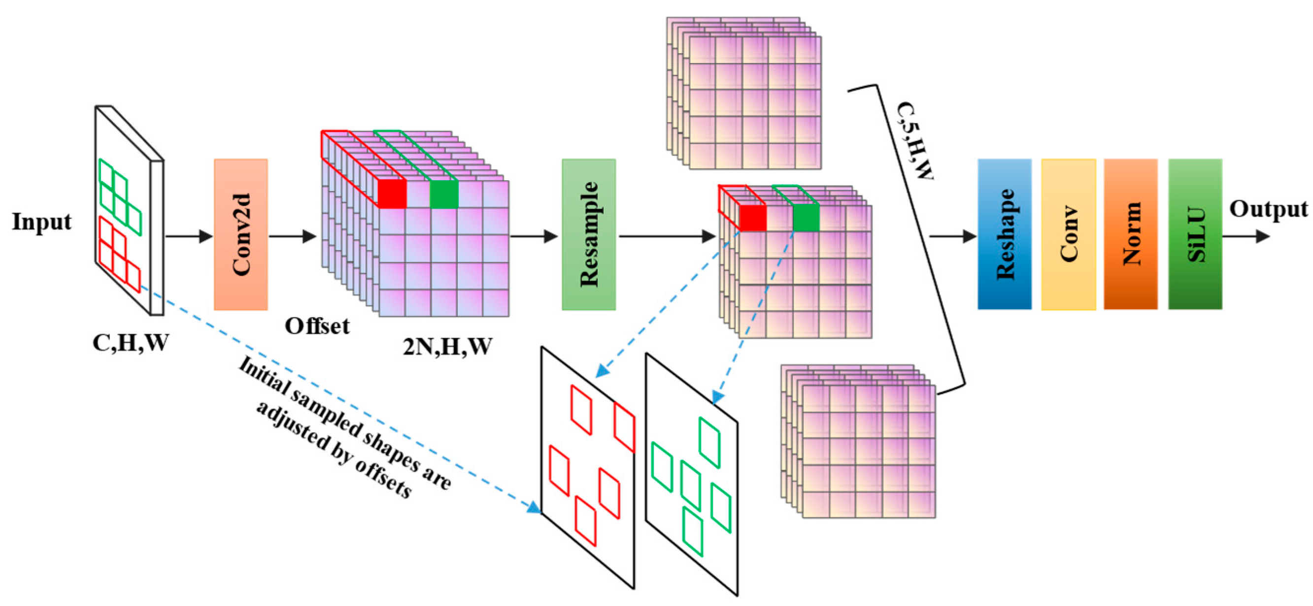
3.3.1. Adaptive Kernel Convolution Module (AKConv)

To address the limitations of fixed standard convolutional sampling shapes, recent studies [22,23] have introduced a novel approach called adaptive kernel convolution (AKConv). This method allows for an arbitrary number of parameters and sampling shapes, thereby enhancing the flexibility and accuracy of feature extraction processes. AKConv utilizes an innovative coordinate generation algorithm to determine the initial positions of convolutional kernels of varying sizes and incorporates an offset mechanism to accommodate target variations, thereby modifying the sampling shape at each position. By implementing irregular convolution operations, AKConv facilitates efficient feature extraction, enabling convolution operations to adapt more effectively to diverse datasets and targets at various spatial locations.

The AKConv architecture is illustrated in Figure 6. The employment of distinct initial sampling shapes for the $5\times 5$ sampling grid by AKConv enables the accurate coverage and processing of diverse image regions, thereby enhancing the precision of feature extraction. The input image is characterized as a three-dimensional feature map, defined by the dimensions C, H, and W. Here, C signifies the number of channels, while H and W correspond to the height and width of the image, respectively.

Initially, AKConv identified the initial sampling position of the convolution kernel using a coordinate generation algorithm and established the sampling shape of the convolution kernel. Subsequently, a depth-2 convolutional layer (Conv2d) performed a convolution operation on the input image. The offset operation then modified the initial sampling shape with a learned offset, allowing for the adaptive adjustment of the kernel shape to align better with the input image’s characteristics. Next, resampling occurred, in which the feature map was resampled according to the modified sampling shape. The adjusted sampling shapes and points facilitated a more flexible capture of local feature variations. Post-processing was performed, during which the resampled feature map underwent reshaping, convolution, and normalization. Finally, the output was generated using the SiLU activation function.

Remark 4

. AKConv designates initial sampling coordinates for volumes of varying dimensions and modifies the sampling configuration via adjustable offsets that are subject to learning [24]. In comparison to the initial sampling configuration, the sampling shape at each location is altered through the process of resampling, enabling AKConv to adapt its operation in real time based on the image content. This provides convolutional networks with unparalleled flexibility and adaptability, resulting in more efficient convolutional neural networks for processing complex and diverse image data [25].

Remark 5.

AKConv enables linear variation in the convolution parameters in contrast to the conventional quadratic growth trajectory [26]. It offers a method to decrease the number of parameters and the computational burden of the model while maintaining performance integrity. This capability not only makes AKConv an effective tool for high-precision feature extraction but also confers significant computational efficiency and lightweight model advantages in underwater docking applications.

3.3.2. Context Aggregation Network (CONTAINER)

In a previous study, Gao et al. proposed a general-purpose network module, designated CONTAINER, for multi-head contextual aggregation [27]. This approach not only employs long-range interactions similar to those observed in transformers but also leverages the inductive bias of local convolution operations to achieve accelerated convergence. Building on this literature, we introduced the CONTAINER module into the YOLO-D framework. This integration enabled the network to effectively combine local and global information, enhancing the contextual information and feature refinement for long-range light and AprilTag detection, as well as other small targets. Consequently, the performance of the model in small-target detection was significantly improved.

When an image is provided as input, it is denoted by $X\in {\mathbb{R}}^{C\times H\times W}$, where $C$ represents the number of channels, and $H\times W$ indicates the spatial dimensions of the image. This image can be transformed into a sequence of tokens, represented as $\left\{X_i\in {\mathbb{R}}^C|i=1,\dots ,N\right\}$, where $N=HW$.

To establish the affinity matrix denoted as $\mathcal{A}\in {\mathbb{R}}^{N\times N}$, within the dimensions $N\times N$, it was essential to characterize the neighborhood for contextual aggregation. This matrix plays a critical role in governing the propagation of information within a feature space. The aggregation function was expressed as follows:

$$Y=\left(\mathcal{A}V\right)W_1+X,$$

(2)

where $V\in {\mathbb{R}}^{N\times C}$ is the matrix transformed by the linear projection $V=X{W}_2$; $W_1$ and $W_2$ are learnable parameters; and ${\mathcal{A}}_{ij}$ is the affinity value between $X_i$ and $X_j$.

To enhance modeling capabilities, multiple affinity matrices were employed to generate a diverse array of pathways that integrated contextual information. The aggregation function for the multi-headed variant was defined as follows:

$$Y=Concat\left({\mathcal{A}}_1{V}_1,\dots ,{\mathcal{A}}_M{V}_M\right)W_2+X,$$

(3)

where ${\mathcal{A}}_m(m=1,\dots ,M)$ is an affinity matrix representing the different relationships in the feature space, which can improve the representation ability of contextual aggregation compared with the single-headed version.

The essential components of CONTAINER consisted of two distinct types of affinity matrices, each with learnable parameters. The single-headed CONTAINER was characterized in the following manner:

$$Y=\left(\left(\alpha \mathcal{A}\left(X\right)+\beta \mathcal{A}\right)V\right)W_2+X,$$

(4)

where $\mathcal{A}\left(X\right)$ is the dynamic affinity matrix dynamically generated from $X$; $\mathcal{A}$ is the static affinity matrix; and $\alpha$ and $\beta$ are learnable parameters.

As demonstrated in the preceding section, the CONTAINER module provides a versatile and robust method for context aggregation by incorporating static and dynamic affinity matrices with learnable parameters.

Remark 6.

CONTAINER offers a comprehensive methodology for global context aggregation, which effectively balances the preservation of local details with an understanding of the overall image context. Compared to conventional local feature extraction techniques, CONTAINER demonstrates an enhanced ability to capture more nuanced global information, making target features more distinctive, particularly in complex scenarios such as the detection of small targets in underwater imagery. Additionally, the lightweight and adaptable architecture of the model allows for seamless integration into existing target detection frameworks without imposing significant computational burdens.

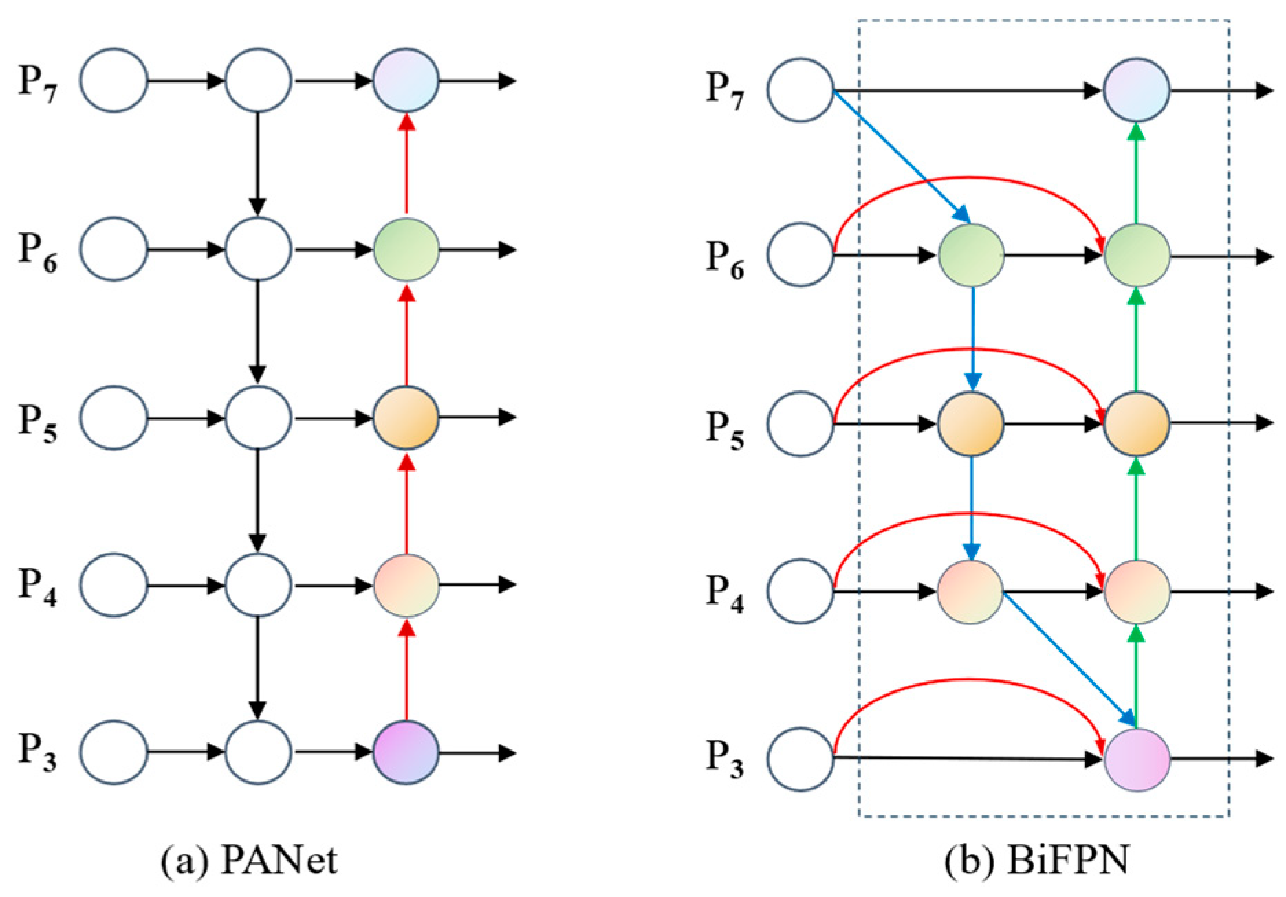
3.3.3. Bidirectional Feature Pyramid Network (BiFPN)

During the underwater docking process, the scale of the landmarks underwent significant alterations and variations owing to changes in distance. However, the capability of a single-layer convolutional neural network to represent feature maps is inherently limited. Therefore, it was essential to develop effective strategies for representing and processing multi-scale features. The conventional top-down Feature Pyramid Network (FPN) can be fundamentally restricted by the unidirectional flow of information [28]. To address this limitation, the path aggregation network (PANet) incorporates an additional bottom-up path aggregation network [29]. In the context of underwater image target detection, numerous images have inadequate resolution and clarity. Consequently, PANet proved insufficient for effective feature extraction, resulting in inaccuracies in the target localization.

In Figure 7, the network structure employed by PANet and the BiFPN for the fusion of features (P3–P7) across different scales is illustrated. The input features at levels 3–7 are represented as ${\overrightarrow{P}}^{in}=\left(P_3^{in},...P_7^{in}\right)$, where $P_i^{in}$ denotes the feature level with a resolution equivalent to the input image $1/2^i$. For instance, if the input resolution is set to $640\times 640$, then $P_3^{in}$ represents the feature layer 3 with a resolution of $80\times 80$. PANet employs an up-down bidirectional path for fusion, while the BiFPN focuses on efficient bidirectional cross-scale connection and weighted feature fusion.

Figure 7b illustrates a bidirectional feature pyramid network (BiFPN), which is distinguished by its bidirectional weighted architecture. This network enhances the integration of comprehensive feature information by eliminating specific input nodes and reinforcing interconnections among nodes within the same layer. The BiFPN effectively optimizes cross-scale connections, facilitating the rapid and efficient fusion of multi-scale features [30,31]. In contrast to the path aggregation network (PANet), which comprises a single top-down and bottom-up pathway, the BiFPN treats each bidirectional pathway as a distinct feature network layer and iteratively applies the same layer multiple times to achieve a more advanced level of feature fusion.

The bidirectional feature pyramid network (BiFPN) employs learnable weights to determine the significance of disparate input features while repeatedly applying a combination of top-down and bottom-up multi-scale feature fusion. The BiFPN facilitates effective bidirectional cross-scale connections and weighted feature fusion. By extending the Feature Pyramid Network (FPN) with bidirectional connections between pyramid levels, the BiFPN enables information to flow both bottom-up and top-down through the network.

A BiFPN utilizes feature weights of different magnitudes as parameters within the context of deep learning [32]. This method of feature fusion is referred to as fast normalized fusion, and its formulation is presented in the following Equation (5).

$$O={\sum }_i{\displaystyle \frac{w_i}{ϵ+{\sum }_j{w}_j}}\cdot I_i,$$

(5)

where $I_i$ and $O$ represent the features before and after fusion, respectively, and $w_i$ and $w_j$ represent the weights of the features to be learned. A value of $ϵ$ that is much less than 1 can contribute to the stability of the system.

Upon completion of the processing phase, the final feature map was produced through the implementation of bidirectional scale connections and effective normalized fusion. The equation used to compute the two integrated features within the BiFPN framework is as follows. The BiFPN incorporates bidirectional cross-scale connections and fast normalized fusion. As a concrete example, we describe here the two fusion features of the sixth layer of the BiFPN shown in Figure 7b:

$$P_6^{td}=Conv\left({\displaystyle \frac{w_1\cdot P_6^{in}+w_2\cdot Resize\left(P_7^{in}\right)}{w_1+w_2+ϵ}}\right),$$

(6)

$$P_6^{out}=Conv\left({\displaystyle \frac{w_1^{\prime }\cdot P_6^{in}+w_2^{\prime }\cdot P_6^{td}+w_3^{\prime }\cdot Resize\left(P_5^{out}\right)}{w_1^{\prime }+w_2^{\prime }+w_3^{\prime }+ϵ}}\right),$$

(7)

where $P_6^{td}$ and $P_6^{out}$ represent the intermediate transition feature of the sixth layer on the top-down path and the final output feature of the sixth layer on the bottom-up path, respectively. In Equation (6), $w_i$ represents the weight parameter necessary to calculate the intermediate transition feature, which serves as both input to the current layer and input to the next layer. In Equation (7), $w_i^{\prime }$ denotes the weights of the current layer’s input, the transition unit’s output of the current layer, and the previous layer’s output, respectively. The term $ϵ$ is a hyperparameter that prevents the gradient from vanishing. All remaining features are developed using a comparable methodology.

The YOLO-D network architecture can be enhanced by incorporating a BiFPN, which facilitates efficient and straightforward multi-scale feature fusion. This enhancement can significantly increase the detection accuracy for small targets located at substantial distances and those obscured. In addition, it can improve the contextual understanding of targets, thereby diminishing the occurrence of both false positives and false negatives.

3.4. Position and Pose Calculation Methods

3.4.1. Camera Models

The underwater camera model comprised four coordinate system transformations (Figure 8). These included the global coordinate system $O_w{-X}_w{Y}_w{Z}_w$, the camera coordinate system $O_c{-X}_c{Y}_c{Z}_c$, the image coordinate system $O_I-X_I{Y}_I$ and the pixel coordinate system $o-uv$. The orange rectangle in the figure represents the camera.

The relationship governing the transformation between the midpoint $P(x_w,y_w,z_w)$ in the world coordinate system and its corresponding projected point $p(u,v)$ in the pixel coordinate system is given by the following Equation [33]:

$$z_c\left[\begin{array}{c}u\\ v\\ 1\end{array}\right]=\left[\begin{array}{cccc}{f}_x& 0& c_x& 0\\ 0& f_y& c_y& 0\\ 0& 0& 1& 0\end{array}\right]\left[\begin{array}{cc}R& t\\ 0^T& 1\end{array}\right]\left[\begin{array}{c}{x}_w\\ y_w\\ z_w\\ 1\end{array}\right]=M_1{M}_2{x}_w=M{x}_w,$$

(8)

where $R$ is a 3 × 3 rotation matrix; $t$ is a 3 × 1 translation matrix; $M_1$ is the intrinsic parameter matrix of the camera; $M_2$ is the extrinsic parameter matrix; $f_x$ and $f_y$ are the equivalent focal lengths in the $x$ and $y$ directions, respectively; $c_x$ and $c_y$ are the optical centers; and $x_w$ is the point coordinate in the world coordinate system.

To enhance detection accuracy, it was essential to account for its nonlinear characteristics, specifically the camera distortion model.

$$\begin{gathered} D_u={\bar{u}}_d\left(k_1{r}_d^2+k_2{r}_d^4+k_3{r}_d^6\right)+2p_1{\bar{u}}_d{\bar{v}}_d+p_2\left(r_d^2+2{\bar{u}}_d^2\right), \\ {D}_v={\bar{v}}_d\left(k_1{r}_d^2+k_2{r}_d^4+k_3{r}_d^6\right)+p_1\left(r_d^2+2{\bar{v}}_d^2\right)+2p_2{\bar{u}}_d{\bar{v}}_d, \end{gathered}$$

(9)

where the variables ${\bar{u}}_d$, ${\bar{v}}_d$, and $r_d$ are defined as follows: ${\bar{u}}_d=u_d-u_0$, ${\bar{v}}_d=v_d-v_0$, and $r_d=\sqrt{{\bar{u}}_d^2+{\bar{v}}_d^2}$. The coefficients $k_1$, $k_2$, and $k_3$ represent the radial distortion, whereas $p_1$ and $p_2$ denote the tangential distortion. It is generally accepted that $k_3=0$. It was necessary to conduct underwater calibration tests to determine the distortion coefficients of a camera.

3.4.2. Multi-Marker Positioning Methods

The position $R$ and orientation $t$ of the camera were determined from three-dimensional points in the world coordinate system and their corresponding two-dimensional projections in the image coordinate system. Subsequently, it was necessary to address the Perspective-n-Point (PnP) problem [34]. Gong et al. proposed a method using four virtual control points to represent three-dimensional reference points and developed an iterative calculation method known as Efficient Perspective-n-Point (EPnP). Although this method demonstrated enhanced efficiency, it lacked adequate accuracy when the number of points $n=4$ or 5 [35]. Sun et al. employed the Robust Perspective-n-Point (RPnP) method to achieve optimal computational precision for both non-redundant ($n\le 6$) and redundant data points [36].

The RPnP algorithm was employed to estimate the attitude between the unmanned underwater vehicle and the docking station, considering the number of landmark points, calculation accuracy, and computational complexity. In the global coordinate system, the longest side, $P_{i0}{P}_{j0}$, was selected as the axis of rotation, with its center designated as the origin.

The n-dimensional points were partitioned into $(n-2)$ subsets, each of which corresponded to a fourth-order polynomial.

$$\left\{\begin{array}{c}{f}_1\left(x\right)=a_1{x}^4+b_1{x}^3+c_1{x}^2+d_{1}x+e_1=0\\ f_2\left(x\right)=a_2{x}^4+b_2{x}^3+c_2{x}^2+d_{2}x+e_2=0\\ \cdots ,\\ f_{n-2}\left(x\right)=a_{n-2}{x}^4+b_{n-2}{x}^3+c_{n-2}{x}^2+d_{n-2}x+e_{n-2}=0\end{array}\right..$$

(10)

The objective was to ascertain the local minimum of the system of equations by using the least-squares residual. Subsequently, the loss function was defined as follows:

$$F={\sum }_{i=1}^{n-2}{f}_i^2\left(x\right).$$

(11)

The minimum value of $F$ was obtained by determining the root of its derivative.

$$F^{\prime }={\sum }_{i=1}^{n-2}{f}_i\left(x\right)f_i^{\prime }\left(x\right)=0,$$

(12)

where $F^{\prime }$ is a seventh-degree polynomial, and the extreme point $x$ can be solved using the eigenvalue method.

Once the rotation axis was identified, the remaining rotation angle and translation vector could be calculated using the following equations:

$$\left[\begin{array}{ccc}{A}_{2n\times 1}& B_{2n\times 1}& C_{2n\times 4}\end{array}\right]\left[\begin{array}{c}\begin{array}{c}c\\ s\\ t_x\end{array}\\ t_y\\ t_z\\ 1\end{array}\right]=0,$$

(13)

$$A_{2n\times 1}=\left[\begin{array}{c}{u}_1{X}_1{r}_3-Y_1{r}_4-X_1{r}_1+u_1{Y}_1{r}_6\\ v_1{X}_1{r}_3-Y_1{r}_5-X_1{r}_2+v_1{Y}_1{r}_6\\ \cdots \\ \cdots \\ u_n{X}_n{r}_3-Y_n{r}_4-X_n{r}_1+u_n{Y}_n{r}_6\\ v_n{X}_n{r}_3-Y_n{r}_5-X_n{r}_2+v_n{Y}_n{r}_6\end{array}\right],$$

(14)

$$B_{2n\times 1}=\left[\begin{array}{c}{Y}_1{r}_1+u_1{X}_1{r}_6-u_1{Y}_1{r}_3-X_1{r}_4\\ Y_1{r}_2+v_1{X}_1{r}_6-v_1{Y}_1{r}_3-X_1{r}_5\\ \cdots \\ \cdots \\ Y_n{r}_1+u_n{X}_n{r}_6-u_n{Y}_n{r}_3-X_n{r}_4\\ Y_n{r}_2+v_n{X}_n{r}_6-v_n{Y}_n{r}_3-X_n{r}_5\end{array}\right],$$

(15)

$$C_{2n\times 4}=\left[\begin{array}{cccc}-1& 0& u_1& u_1{r}_9{Z}_1-r_7{Z}_1\\ 0& -1& v_1& v_1{r}_9{Z}_1-r_8{Z}_1\\ \cdots & \cdots & \cdots & \cdots \\ \cdots & \cdots & \cdots & \cdots \\ -1& 0& u_n& u_n{r}_9{Z}_n-r_7{Z}_n\\ 0& -1& v_n& v_n{r}_9{Z}_n-r_8{Z}_n\end{array}\right].$$

(16)

The unknown variables $c,s,t_x,t_y,$ and $t_z$ in Equation (13) can be solved by employing singular value decomposition (SVD) to resolve this linear equation system.

4. Experimental Results and Discussion

4.1. Experimental Setup and Datasets

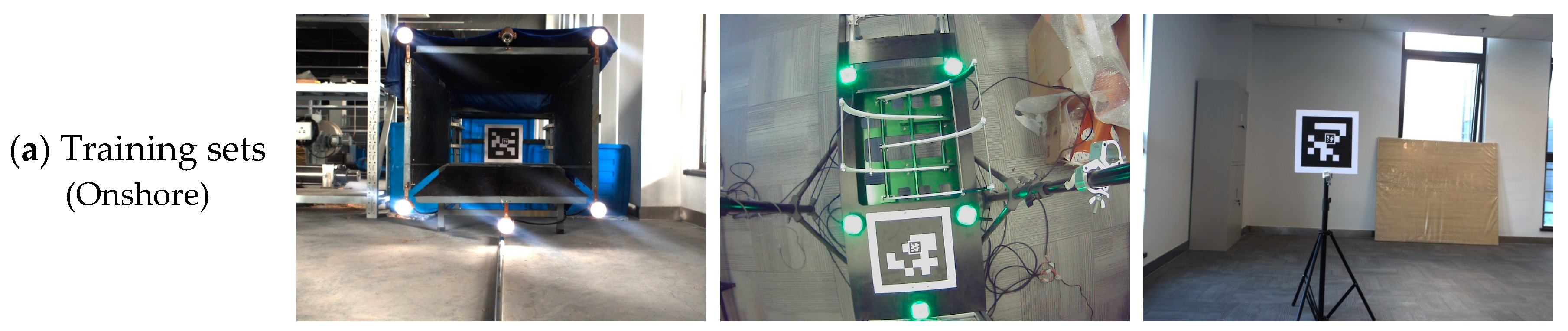
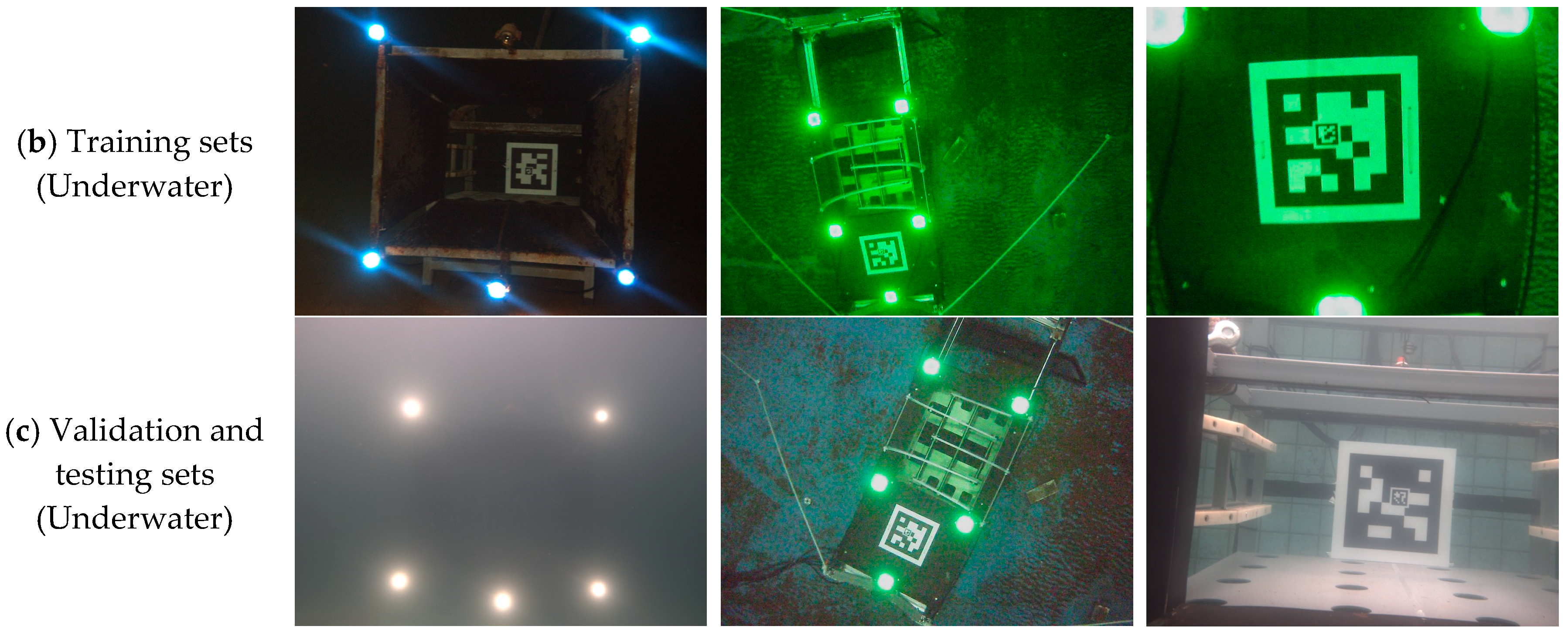
4.1.1. Datasets

Currently, underwater image datasets are scarce compared with other application scenarios, and no publicly available datasets are suitable for underwater docking scenarios. Hence, we developed a custom image dataset for underwater docking markers, which included the guiding light source for underwater docking, the AprilTag marker, two representative types of docking recovery stations (DSs), and other common interference objects. The dataset comprised 240 training samples, 83 validation samples, and 82 test samples, representing approximately 60%, 20%, and 20% of the entire dataset, respectively. As illustrated in Figure 9, the images displayed considerable quality deficiencies, characterized by color discrepancies, blurriness, insufficient contrast, and the presence of overlapping objects.

Underwater testing conditions render capturing images of the underwater docking process challenging, thereby demonstrating the value of the obtained data. Consequently, the number of image samples is relatively limited compared with those available in public datasets. To facilitate model training, we incorporated a subset of marker samples captured in laboratory air into the training set (Figure 9a). We also used a set of different experimental data as training samples. The validation and testing sets consisted of images from actual underwater docking scenes (Figure 9b).

4.1.2. Experimental Setup

• Training Computer Configuration

The computer configuration was utilized for YOLO-D model training, along with the hyperparameter settings employed during the training stage (

Table 1. Table of computer configurations for model training.

Class	Project	Parameter Values
Hardware environment	CPU	16v CPU Intel(R) Xeon(R) Gold 6430
	CPU RAM	120 GB
	GPU	NVIDIA GeForce RTX 4090
	GPU RAM	24 GB
Software environment	Operating system	Ubuntu 18.04
	Programming language	Python v3.8
	Deep learning framework	Pytorch v1.8.1
	CUDA	v11.1
Experimental hyperparameters	Image size	800 × 600
	Learning rate	0.01
	Momentum	0.937
	Weight decay	0.0005
	Batch size	32
	Epoch	300

). Given the typically limited input size of mobile networks, all images were scaled to a uniform size for training.

2.

Embedded Computer Configuration

The underwater docking guidance and detection equipment utilized the NVIDIA Jetson AGX Orin component, and its detailed configuration is presented in

Table 2. Embedded computer configuration table for image detection.

Project	Parameter Values
CPU	12-core Arm® Cortex®-A78AE v8.2 64-bit
GPU	2048-core NVIDIA Ampere architecture GPU with 64 Tensor Cores
AI computing power	275 TOPS
Graphics memory	64 GB LPDDR5
RAM	64 GB
Power range	15–75 W

.

3.

Underwater Camera Configuration

The underwater camera employed a custom configuration for image acquisition in an underwater environment. The specific configurations are listed in

Table 3. Parameter table for underwater cameras.

Project	Parameter Values
Image Resolution	$800\times 600$
Pixel Size	$8.29 \mathsf{\mu }\mathrm{m}\times 8.30 \mathsf{\mu }\mathrm{m}$
Maximum Frame Rate	40 fps
Data Transfer Interface	USB

.

The calibration test of the underwater camera yielded a focal length of 7.109 mm, central pixel coordinates of 417.582 and 285.199, and radial distortion coefficients of $k_1=7093.46$, $k_2=3.96219\times {10}^6$, and $k_3=3.88195\times {10}^{12}$. The tangential distortion coefficients were $p_1=0.0249934$ and $p_2=0.374426$. Additionally, the docking guide was illuminated by a custom-built underwater LED light source with a maximum power output of 35 W, with its brightness adjusted as needed.

4.1.3. Evaluation Metrics

In the domain of image target detection, performance metrics can be primarily divided into accuracy and speed metrics. This study employed five metrics to assess the performance of the underwater detection model: precision, recall, F1 score, mean average precision (mAP@0.5), and frames per second (FPS) [37,38]. The first four are accuracy metrics, with precision ascertaining the accuracy of markers detection, recall assessing the capacity to identify all signs, the F1 score providing a comprehensive evaluation of accuracy and recall, and mAP evaluating the accuracy of model detection. The speed metric FPS can measure the speed of object detection by determining the number of images processed per second [39]. The evaluation metrics were calculated as follows:

$$Precision={\displaystyle \frac{TP}{TP+FP}}\times 100\%,$$

(17)

$$Recall={\displaystyle \frac{TP}{FN+TP}}\times 100\%,$$

(18)

$$F1Score=2\times {\displaystyle \frac{Precision\times Recall}{Precision+Recall}},$$

(19)

$$AP={\int }_0^{1}P\left(R\right)dR,$$

(20)

$$mAP={\displaystyle \frac{1}{n}}{\sum }_{i=0}^{n}AP.$$

(21)

For object detection, TP denotes the number of correctly identified signs, FP denotes the number of incorrectly identified signs, TN denotes the number of undetected signs, FN denotes the number of missed signs, and $n$ represents the number of classes. mAP@0.5 refers to the average AP for all categories when IoU is greater than or equal to 0.5. Conversely, mAP@0.5:0.95 represents the average mAP across a range of IoU thresholds, from 0.5 to 0.95.

4.2. Comparison Experiments

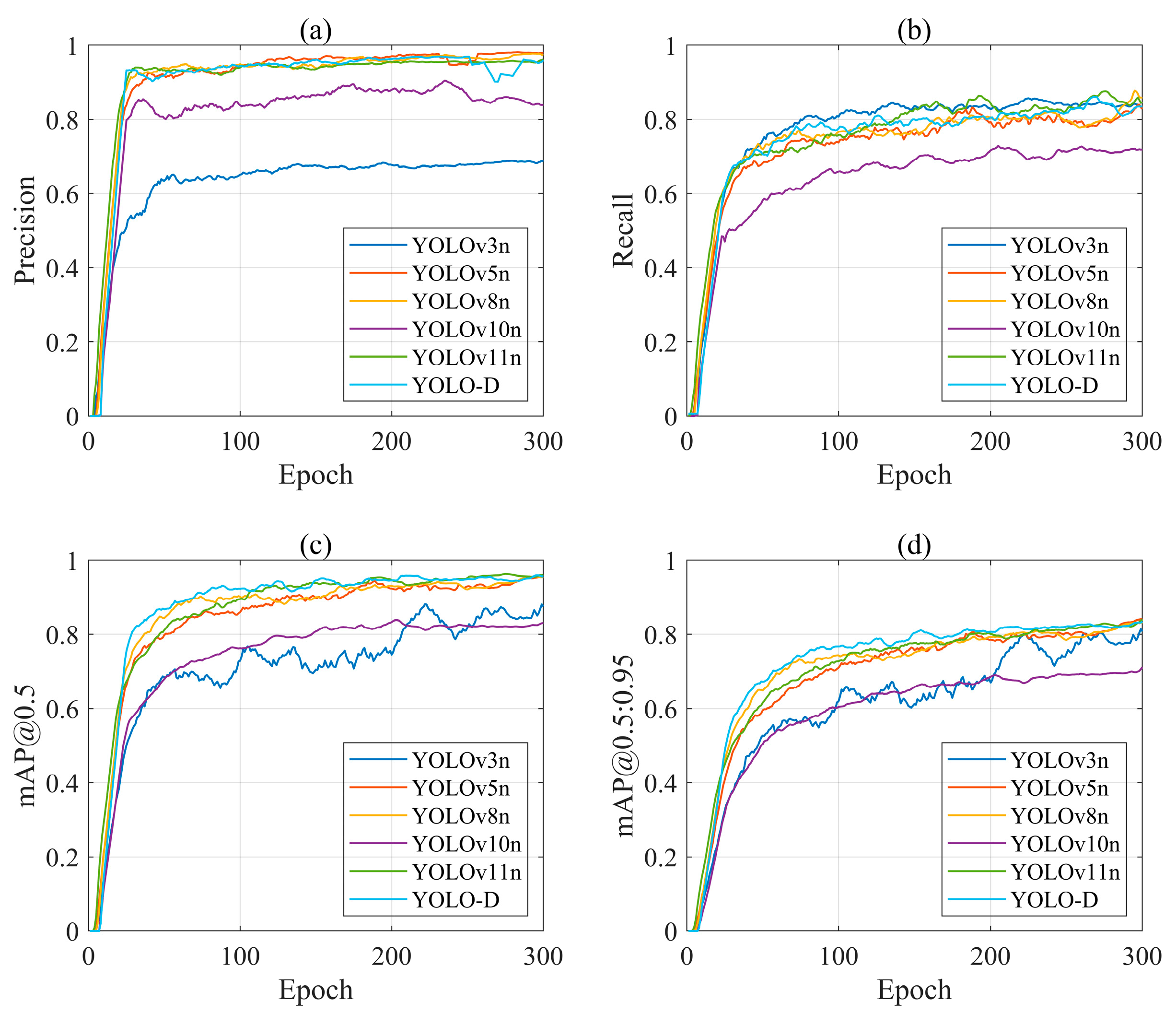
4.2.1. Comparison of Training Processes

The following section presents a comparative analysis of the proposed YOLO-D network against current mainstream object detection networks known for their excellent detection performance. Comparative testing included the models YOLOv3n, YOLOv5n, YOLOv8n, YOLOv10n, and the original version of YOLOv11n. Notably, all networks were trained and tested using the same settings.

Figure 10 illustrates the total loss function curves of the improved YOLO-D model and comparison models for the training and validation sets. The training outcomes indicated that all four models exhibited a swift decline in the value of the loss function during the initial stages of training. Up to approximately the 60th epoch, the loss values of each model declined gradually, approaching approximately 2.6. Finally, the loss curves stabilized, with the loss values settling at approximately 1.5, indicating that each model achieved excellent convergence.

Figure 11 presents the precision, recall, mAP@0.5, and mAP@0.5:0.95 curves obtained from YOLO-D and the comparison models during the training process. After 300 training epochs, except for YOLOv3n and YOLOv10n, all models exhibited a satisfactory level of fitting, which exhibited no significant signs of overfitting or underfitting. The YOLO-D model exhibited a notable capacity for effective convergence, accompanied by a more stable range of fluctuations in loss. The training results indicated that YOLO-D achieved a maximum precision of 98.5%, maximum recall of 95.6%, mAP@0.5 of 97.7%, and mAP@0.5:0.95 of 84.7% on the training set. Compared to the baseline model YOLOv11n, the precision remained approximately equivalent, while the recall improved by 1%, mAP@0.5 increased by 1.3%, and mAP@0.5:0.95 increased by 0.7%. These training results demonstrate that YOLO-D offers advantages in terms of recall and mAP@0.5, thereby significantly enhancing the stability of the underwater docking algorithm.

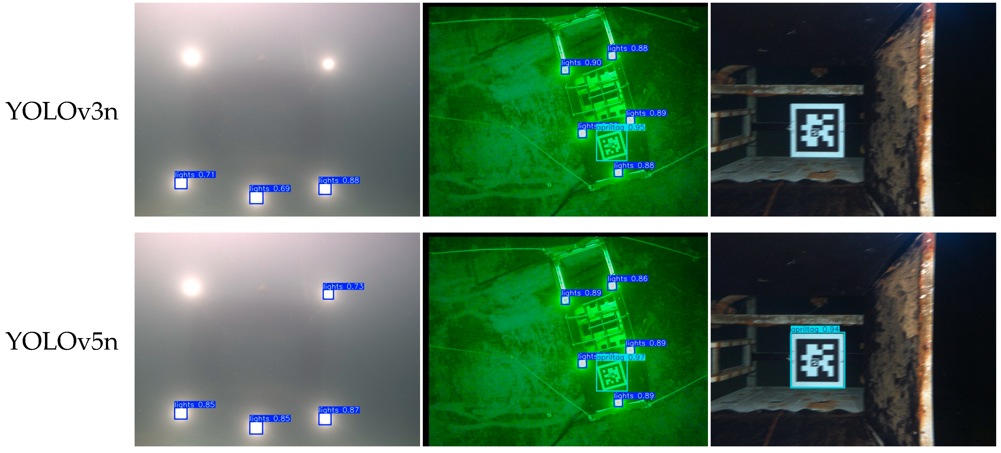
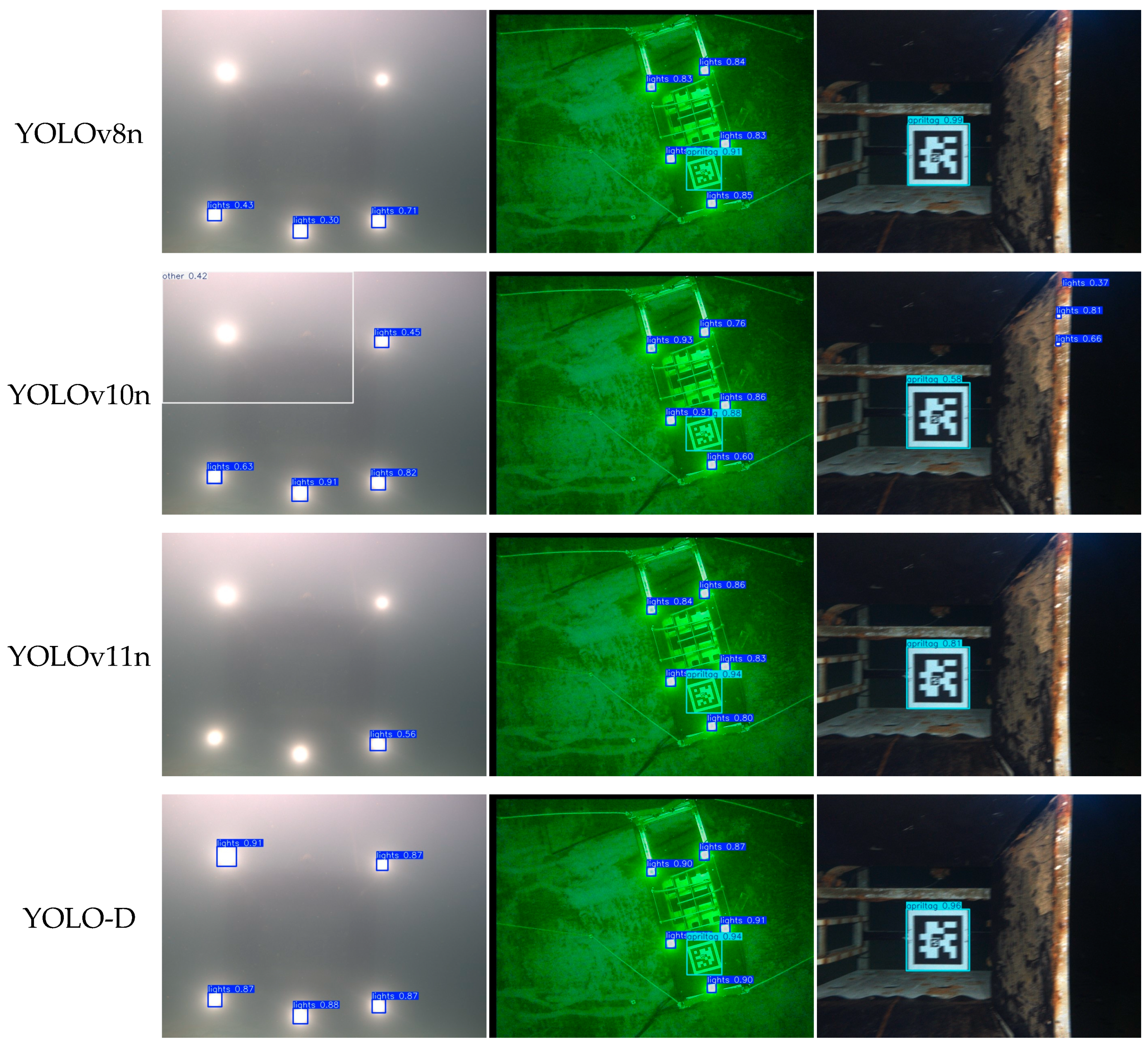
4.2.2. Comparative Tests for Target Detection

To further verify the effectiveness and performance of the YOLO-D detection model, a comprehensive comparison was conducted between the proposed YOLO-D model and various comparison models in terms of average detection accuracy, F1 score, and detection speed on the testing set. The precision–recall (P-R) curves of the different models are shown in Figure 12.

A series of comparative experiments on docking marker detection was conducted on the testing set.

Table 4. Comparison of model evaluation metrics for underwater docking object detection.

Case	Models	Precision	Recall	F1 Score	mAP@ 0.5	mAP@ 0.5:0.95	Parameters (M)	Speed (FPS)
1	YOLOv3n	94.90%	79.70%	86.64%	90.50%	80.00%	103.67	56.50
2	YOLOv5n	96.30%	79.10%	86.86%	91.10%	79.10%	2.50	101.01
3	YOLOv8n	93.00%	83.90%	88.22%	92.80%	80.80%	3.01	103.09
4	YOLOv10n	95.40%	73.30%	82.90%	84.80%	72.90%	2.70	90.91
5	YOLOv11n	95.90%	79.20%	86.75%	90.30%	77.70%	2.58	95.24
6	YOLO-D	97.40%	84.20%	90.32%	94.50%	84.10%	3.03	61.35

presents the accuracy, performance, computational cost, and model size of the various models. YOLO-D achieved a maximum detection precision of 97.4%, a maximum recall of 84.2%, an F1 score of 90.32%, and a mAP@0.5 of 94.50%. YOLO-D demonstrated superior detection precision and recall compared with the other models, including YOLOv3n, YOLOv5n, YOLOv8n, YOLOv10n, and YOLOv11n. When benchmarked against the second-best performing model YOLOv8n, YOLO-D exhibited a 4.4% improvement in precision, a 1.7% improvement in mAP@0.5, and a 2.1% enhancement in the F1 score. The analysis indicates that the YOLO-D model exhibits superior performance on the training dataset while also demonstrating exceptional detection capabilities on novel and previously unencountered testing set data. It is noteworthy that, in comparison with YOLOv8n, YOLOv11n enhances precision by 2.9%, concurrently reducing parameters by 14.3%. This indicates that YOLOv11n further reduces the computational burden while maintaining efficient performance, a critical consideration for underwater docking applications.

Regarding the speed of detection, the YOLO-D model achieved 61.35 Hz, which was slightly lower than that of the other models. However, this speed was sufficient to satisfy the requirements of underwater docking guidance. Regarding model lightweighting, the YOLO-D model had a size of 3.03 M, which was comparable to other models and suitable for deployment and application in embedded control systems.

The data in Table 4 can more accurately reflect the true performance of various methods in a statistical sense. To facilitate a more intuitive comprehension of the effect of image target detection using various methods, three typical representative images were selected from 82 test samples, and the detection results are shown in Figure 13. Figure 13 presents the comparison test results for the testing set as determined by the detection models. The proposed YOLO-D model exhibited superior performance in terms of detection accuracy and F1 score compared with the other models under consideration. With regard to precision, YOLO-D demonstrated a 1.1% higher performance than the second-best YOLOv5n, and in terms of the F1 score, it exhibited a 2.1% higher performance than the second-best YOLOv8n.

In contrast, models such as YOLOv3n and YOLOv10n tended to produce false positives and negatives. Additionally, the YOLO-D model significantly enhanced the reliability of the detection boxes for two distinct categories of valid targets: lights and AprilTag.

4.3. Ablation Experiments

Ablation experiments were performed to analyze the performance differences resulting from various combinations of the enhancement modules in the YOLO-D model. YOLOv11n was adopted as the baseline model to compare the performances of the modules developed in this study. To ensure fairness, the same initial settings were applied during training.

Enhancement modules, including the BiFPN, AKConv, and CONTAINER, were gradually incorporated into the system. To evaluate the efficacy of each proposed module, a series of experiments was conducted on the testing set using various detection metrics. The results of the ablation experiments are presented in

Table 5. Comparison of model evaluation metrics of ablation experiments.

Case	Models				Precision	Recall	F1 Score	mAP @0.5	Parameters (M)
	Baseline	BiFPN	AKConv	Container
1	√				95.90%	79.20%	86.75%	90.30%	2.58
2	√	√			92.20%	81.50%	86.52%	91.90%	2.58
3	√		√		95.00%	80.50%	87.15%	90.50%	2.28
4	√			√	96.20%	80.00%	87.36%	91.30%	3.33
5	√	√	√		95.50%	83.40%	89.04%	90.70%	2.28
6	√	√		√	96.20%	83.70%	89.52%	92.80%	3.33
7	√		√	√	95.50%	80.50%	87.36%	91.50%	3.03
8	√	√	√	√	97.40%	84.20%	90.32%	94.50%	3.03

, where the bold text highlights the optimal results achieved after experimental modifications. The symbol “√” indicates the implementation of a specific strategy.

The findings in Table 5 indicate that the enhanced YOLOv11n model outperformed the baseline model across all evaluated metrics, demonstrating the effectiveness of the proposed architectural integration of the three modules. Compared to the baseline YOLOv11n model, the YOLO-D architecture achieved a 1.5% improvement in precision, a 5% enhancement in recall, a 4.2% increase in mAP@0.5, and a 3.57% increase in the F1 score. However, the inclusion of these additional modules resulted in a 17.44% increase in model parameters.

The results of the ablation experiment demonstrated that the YOLO-D architecture was optimized and balanced in several ways, including improvements in detection accuracy and recall rate, along with a reduction in the overall footprint of the system. The incorporation of the CONTAINER module led to comprehensive enhancements in object detection accuracy and recall rate. The BiFPN module facilitated the extraction of relevant feature information related to the detected object while reducing the influence of irrelevant environmental data and significantly enhancing the recall rate. The AKConv module significantly affected both the recall rate and the model lightweighting. However, the integration of multiple modules resulted in a slight increase in the computational complexity of the model compared with its previous state.

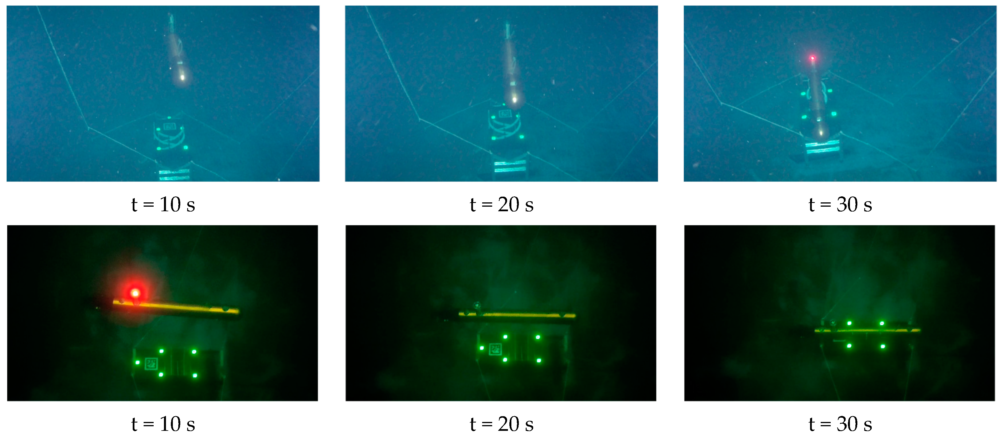
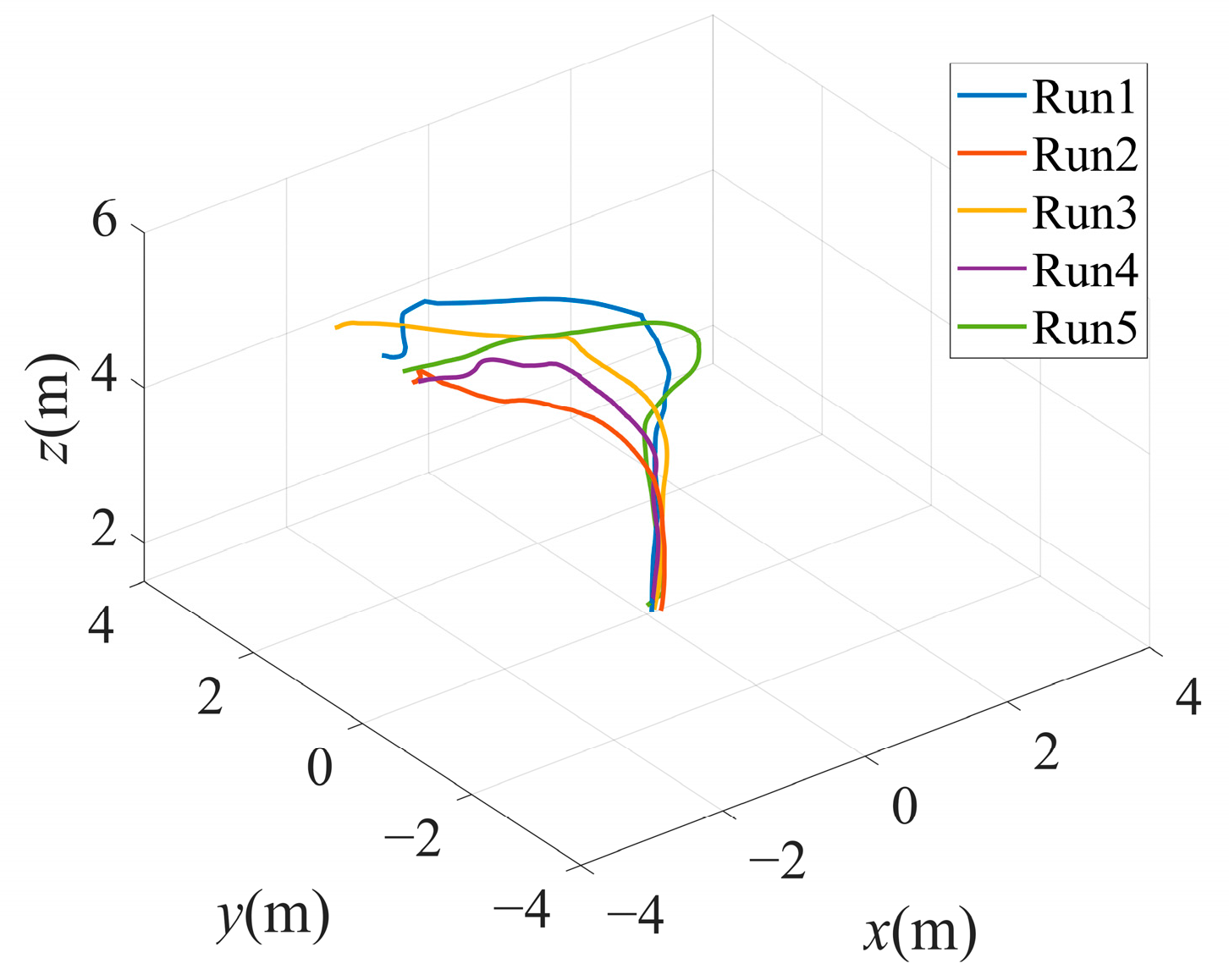
4.4. Underwater Docking Positioning Experiment

To validate the effectiveness of the underwater docking guidance positioning approach proposed in this study further, docking guidance experiments were conducted in a pool environment. The testing process captured from a third-person perspective by the underwater robots is shown in Figure 14.

The proposed visual guidance and positioning methodology for autonomous docking of a UUV was tested in a pool without lighting. In order to assess the efficacy of the proposed underwater guidance and positioning method, we conducted a series of 10 tests in a pool environment. For the purpose of elucidating the experimental findings, we selected five representative datasets from the total of 10 tests conducted. The position–space curve of the underwater landing and docking process based on the five recorded tests is shown in Figure 15. During the experiment, the fixed image acquisition and marker detection frequencies were maintained at 20 Hz, which satisfied the requirements for underwater docking control. The docking guidance and positioning algorithm enabled the UUV to autonomously land and move into the docking device despite varying the initial positions, with a maximum position control error of less than ±20 mm, and the error of the heading angle was less than 3°.

The curves representing the position and attitude of the UUV during underwater docking from various initial positions are shown in Figure 16. Figure 16a–d illustrate the longitudinal displacement $\xi$, transverse displacement $\eta$, vertical displacement $\zeta$, and heading angle $\psi$ of the UUV relative to the DS, as measured by the visual guidance positioning system. The results of the underwater docking pool tests were satisfactory, with ten consecutive docking experiments conducted and a success rate of approximately 90%. The pool tests verified the effectiveness of the designed visual guidance positioning control system. The primary reason for unsuccessful docking was determined to be the impact of water flow disturbances on docking motion control.

Although progress has been made in the autonomous underwater docking control method, this study has several limitations, which will be addressed in future work. This study is deficient in three key areas.

• The current dataset requires improvement in both quantity and quality, owing to the challenges of capturing underwater docking images. In addition, data enhancement methods can be used to improve the precision and recall of underwater target detection.
• Although YOLO-D incorporated the BiFPN architecture to enhance the feature fusion capabilities, the detection and processing efficiency of underwater micro-small targets remained a significant challenge. Therefore, further research on more advanced architectures is required to address this issue.
• The proposed algorithm imposed high demands on the inferencing capabilities of device hardware. Future research will focus on model lightweighting to enhance computational performance and reduce hardware dependence. This will enable deployment in low-cost embedded systems while simultaneously lowering the power consumption of underwater unmanned equipment control systems.

5. Conclusions

This study proposed a novel method for underwater landing guidance and positioning based on machine vision and deep learning. A cascaded guidance and positioning strategy was developed by combining an active light array with a passive AprilTag, thereby offering an extended effective range and high guidance accuracy. The YOLO-D model was introduced for marker detection under complex underwater visual conditions, integrating bidirectional feature pyramid networks (BiFPN) to facilitate cross-scale connections and learnable weights, thus enhancing multi-scale target feature fusion. To address the unique characteristics of lights and AprilTag, the AKConv module adaptively adjusted the shape and size of the convolutional kernels, improving the feature extraction accuracy and efficiency. Additionally, the CONTAINER mechanism was incorporated to enhance the feature extraction for small, long-distance targets. Comparative experiments on underwater target recognition and ablation studies demonstrated that YOLO-D significantly outperformed the baseline model YOLOv11n in terms of detection accuracy and recall rate. Although the detection speed was slightly lower than that of the baseline model, it satisfied the requirements for underwater docking guidance and positioning. The pool tests confirmed the feasibility and effectiveness of the proposed method. Future research will explore transfer learning techniques and the collection of laboratory datasets to train models for underwater scene target detection, further enhancing the applicability and detection accuracy of the algorithm.

References

1. Khan, A.; Fouda, M.M.; Do, D.-T.; Almaleh, A.; Alqahtani, A.M.; Rahman, A.U. Underwater target detection using deep learning: Methodologies, challenges, applications and future evolution. IEEE Access 2024, 12, 12618–12635. [Google Scholar] [CrossRef]
2. Xu, Z.; Haroutunian, M.; Murphy, A.J.; Neasham, J.; Norman, R. An underwater visual navigation method based on multiple ArUco markers. J. Mar. Sci. Eng. 2021, 9, 1432. [Google Scholar] [CrossRef]
3. Yan, Z.; Gong, P.; Zhang, W.; Li, Z.; Teng, Y. Autonomous Underwater Vehicle Vision Guided Docking Experiments Based on L-Shaped Light Array. IEEE Access 2019, 7, 72567–72576. [Google Scholar] [CrossRef]
4. Wang, Y.; Ma, X.; Wang, J.; Wang, H. Pseudo-3D vision-inertia based underwater self-localization for AUVs. IEEE Trans. Veh. Technol. 2020, 69, 7895–7907. [Google Scholar] [CrossRef]
5. Lv, F.; Xu, H.; Shi, K.; Wang, X. Estimation of Positions and Poses of Autonomous Underwater Vehicle Relative to Docking Station Based on Adaptive Extraction of Visual Guidance Features. Machines 2022, 10, 571. [Google Scholar] [CrossRef]
6. Trslić, P.; Weir, A.; Riordan, J.; Omerdic, E.; Toal, D.; Dooly, G. Vision-based localization system suited to resident underwater vehicles. Sensors 2020, 20, 529. [Google Scholar] [CrossRef]
7. Pan, W.; Chen, J.; Lv, B.; Peng, L. Optimization and Application of Improved YOLOv9s-UI for Underwater Object Detection. Appl. Sci. 2024, 14, 7162. [Google Scholar] [CrossRef]
8. Liu, K.; Peng, L.; Tang, S. Underwater object detection using TC-YOLO with attention mechanisms. Sensors 2023, 23, 2567. [Google Scholar] [CrossRef]
9. Wang, Z.; Zhang, G.; Luan, K.; Yi, C.; Li, M. Image-fused-guided underwater object detection model based on improved YOLOv7. Electronics 2023, 12, 4064. [Google Scholar] [CrossRef]
10. Wang, L.; Ye, X.; Wang, S.; Li, P. ULO: An underwater light-weight object detector for edge computing. Machines 2022, 10, 629. [Google Scholar] [CrossRef]
11. Chen, X.; Fan, C.; Shi, J.; Wang, H.; Yao, H. Underwater target detection and embedded deployment based on lightweight YOLO_GN. J. Supercomput. 2024, 80, 14057–14084. [Google Scholar] [CrossRef]
12. Zhang, M.; Xu, S.; Song, W.; He, Q.; Wei, Q. Lightweight underwater object detection based on yolo v4 and multi-scale attentional feature fusion. Remote Sens. 2021, 13, 4706. [Google Scholar] [CrossRef]
13. Chen, Y.; Zhao, F.; Ling, Y.; Zhang, S. YOLO-Based 3D Perception for UVMS Grasping. J. Mar. Sci. Eng. 2024, 12, 1110. [Google Scholar] [CrossRef]
14. Li, Y.; Liu, W.; Li, L.; Zhang, W.; Xu, J.; Jiao, H. Vision-based target detection and positioning approach for underwater robots. IEEE Photonics J. 2022, 15, 8000112. [Google Scholar] [CrossRef]
15. Liu, S.; Ozay, M.; Xu, H.; Lin, Y.; Okatani, T. A Generative Model of Underwater Images for Active Landmark Detection and Docking. In Proceedings of the 2019 IEEE/RSJ International Conference on Intelligent Robots and Systems (IROS), Macau, China, 3–8 November 2019. [Google Scholar]
16. Lwin, K.N.; Mukada, N.; Myint, M.; Yamada, D.; Yanou, A.; Matsuno, T.; Saitou, K.; Godou, W.; Sakamoto, T.; Minami, M. Visual docking against bubble noise with 3-D perception using dual-eye cameras. IEEE J. Ocean. Eng. 2018, 45, 247–270. [Google Scholar] [CrossRef]
17. Sun, K.; Han, Z. Autonomous underwater vehicle docking system for energy and data transmission in cabled ocean observatory networks. Front. Energy Res. 2022, 10, 960278. [Google Scholar] [CrossRef]
18. Liu, S.; Xu, H.; Lin, Y.; Gao, L. Visual navigation for recovering an AUV by another AUV in shallow water. Sensors 2019, 19, 1889. [Google Scholar] [CrossRef]
19. Zhang, T.; Li, D.; Lin, M.; Wang, T.; Yang, C. AUV terminal docking experiments based on vision guidance. In Proceedings of the OCEANS 2016 MTS/IEEE Monterey, Monterey, CA, USA, 19–23 September 2016; pp. 1–5. [Google Scholar]
20. Lwin, K.N.; Yonemori, K.; Myint, M.; Yanou, A.; Minami, M. Autonomous docking experiment in the sea for visual-servo type undewater vehicle using three-dimensional marker and dual-eyes cameras. In Proceedings of the 2016 55th Annual Conference of the Society of Instrument and Control Engineers of Japan (SICE), Tsukuba, Japan, 20–23 September 2016. [Google Scholar]
21. Khanam, R.; Hussain, M. YOLOv11: An Overview of the Key Architectural Enhancements. arXiv 2024, arXiv:2410.17725. [Google Scholar]
22. Zhang, X.; Song, Y.; Song, T.; Yang, D.; Ye, Y.; Zhou, J.; Zhang, L. AKConv: Convolutional kernel with arbitrary sampled shapes and arbitrary number of parameters. arXiv 2023, arXiv:2311.11587. [Google Scholar]
23. Zhang, X.; Song, Y.; Song, T.; Yang, D.; Ye, Y.; Zhou, J.; Zhang, L. LDConv: Linear deformable convolution for improving convolutional neural networks. Image Vis. Comput. 2024, 149, 105190. [Google Scholar] [CrossRef]
24. Nie, R.; Shen, X.; Li, Z.; Jiang, Y.; Liao, H.; You, Z. Lightweight Coal Flow Foreign Object Detection Algorithm. In Proceedings of the International Conference on Intelligent Computing, Tianjin, China, 5–8 August 2024; pp. 393–404. [Google Scholar]
25. Qin, X.; Yu, C.; Liu, B.; Zhang, Z. YOLO8-FASG: A High-Accuracy Fish Identification Method for Underwater Robotic System. IEEE Access 2024, 12, 73354–73362. [Google Scholar] [CrossRef]
26. Chen, Z.; Feng, J.; Yang, Z.; Wang, Y.; Ren, M. YOLOv8-ACCW: Lightweight grape leaf disease detection method based on improved YOLOv8. IEEE Access 2024, 12, 123595–123608. [Google Scholar] [CrossRef]
27. Gao, P.; Lu, J.; Li, H.; Mottaghi, R.; Kembhavi, A. Container: Context aggregation network. arXiv 2021, arXiv:2106.01401. [Google Scholar]
28. Tan, M.; Pang, R.; Le, Q.V. Efficientdet: Scalable and efficient object detection. In Proceedings of the IEEE/CVF Conference on Computer Vision and Pattern Recognition, Seattle, WA, USA, 13–19 June 2020; pp. 10781–10790. [Google Scholar]
29. Liu, S.; Qi, L.; Qin, H.; Shi, J.; Jia, J. Path aggregation network for instance segmentation. In Proceedings of the IEEE Conference on Computer Vision and Pattern Recognition, Salt Lake City, UT, USA, 18–23 June 2018; pp. 8759–8768. [Google Scholar]
30. Ma, D.; Yang, J. Yolo-animal: An efficient wildlife detection network based on improved yolov5. In Proceedings of the 2022 International Conference on Image Processing, Computer Vision and Machine Learning (ICICML), Xi’an, China, 28–30 October 2022; pp. 464–468. [Google Scholar]
31. Zhang, Z.; Lu, X.; Cao, G.; Yang, Y.; Jiao, L.; Liu, F. ViT-YOLO: Transformer-based YOLO for object detection. In Proceedings of the IEEE/CVF International Conference on Computer Vision, Montreal, BC, Canada, 11–17 October 2021; pp. 2799–2808. [Google Scholar]
32. Du, B.; Wan, F.; Lei, G.; Xu, L.; Xu, C.; Xiong, Y. YOLO-MBBi: PCB surface defect detection method based on enhanced YOLOv5. Electronics 2023, 12, 2821. [Google Scholar] [CrossRef]
33. Kim, J.-Y.; Kim, I.-S.; Yun, D.-Y.; Jung, T.-W.; Kwon, S.-C.; Jung, K.-D. Visual Positioning System Based on 6D Object Pose Estimation Using Mobile Web. Electronics 2022, 11, 865. [Google Scholar] [CrossRef]
34. Wang, P.; Xu, G.; Cheng, Y.; Yu, Q. A simple, robust and fast method for the perspective-n-point problem. Pattern Recognit. Lett. 2018, 108, 31–37. [Google Scholar] [CrossRef]
35. Gong, X.; Lv, Y.; Xu, X.; Wang, Y.; Li, M. Pose Estimation of Omnidirectional Camera with Improved EPnP Algorithm. Sensors 2021, 21, 4008. [Google Scholar] [CrossRef] [PubMed]
36. Sun, Y.; Xia, X.; Xin, L.; He, W. RPnP Pose Estimation Optimized by Comprehensive Learning Pigeon-Inspired Optimization for Autonomous Aerial Refueling. In Proceedings of the International Conference on Guidance, Navigation and Control, Tianjin, China, 5–7 August 2022; pp. 6117–6124. [Google Scholar]
37. Guo, Y.; Chen, S.; Zhan, R.; Wang, W.; Zhang, J. Sar ship detection based on yolov5 using cbam and bifpn. In Proceedings of the IGARSS 2022–2022 IEEE International Geoscience and Remote Sensing Symposium, Kuala Lumpur, Malaysia, 17–22 July 2022; pp. 2147–2150. [Google Scholar]
38. Liu, X.; Chu, Y.; Hu, Y.; Zhao, N. Enhancing Intelligent Road Target Monitoring: A Novel BGS YOLO Approach Based on the YOLOv8 Algorithm. IEEE Open J. Intell. Transp. Syst. 2024, 5, 509–519. [Google Scholar] [CrossRef]
39. Zhao, S.; Zheng, J.; Sun, S.; Zhang, L. An improved YOLO algorithm for fast and accurate underwater object detection. Symmetry 2022, 14, 1669. [Google Scholar] [CrossRef]
Figure 1. Schematic of underwater vertical docking: (a) coordinate system of UUV; (b) arrangement and visual field of the camera; (c) coordinates of docking station; (d) final docking status.
Jmse 13 00102 g001
Figure 2. Underwater vertical docking guidance and positioning system: (a) unmanned underwater vehicle designed for docking; (b) docking station.
Jmse 13 00102 g002
Figure 3. Underwater docking guidance and positioning software structure.
Jmse 13 00102 g003
Figure 4. YOLOv11 network structure.
Jmse 13 00102 g004
Figure 5. YOLO-D network structure.
Jmse 13 00102 g005
Figure 6. Structure diagram of AKConv.
Jmse 13 00102 g006
Figure 7. PANet and BiFPN structure: (a) PANet structure; (b) BiFPN structure.
Jmse 13 00102 g007
Figure 8. Coordinate system for monocular vision position.
Jmse 13 00102 g008
Figure 9. Samples selected from datasets: (a) training set images captured onshore; (b) training set images taken underwater; (c) validation and testing set images taken underwater.
Jmse 13 00102 g009aJmse 13 00102 g009b
Figure 10. Train and valid total loss curves of different models: (a) train total loss curves; (b) valid total loss curves.
Jmse 13 00102 g010
Figure 11. Comparison of performance metric curves of different models: (a) comparison curves of precision; (b) comparison curves of recall; (c) comparison curves of mAP@0.5; (d) comparison curves of mAP@0.5:0.95.
Jmse 13 00102 g011
Figure 12. Precision–recall curves of different models.
Jmse 13 00102 g012
Figure 13. Comparison of experiment object detection effects.
Jmse 13 00102 g013aJmse 13 00102 g013b
Figure 14. Underwater landing docking guidance and positioning pool test.
Jmse 13 00102 g014
Figure 15. Underwater docking position curves.
Jmse 13 00102 g015
Figure 16. Position and pose curves of underwater docking: (a) position curves of ξ ; (b) position curves of η ; (c) position curves of ζ ; (d) yaw curves of ψ .
Jmse 13 00102 g016