A Robust Cross-Band Network for Blind Source Separation of Underwater Acoustic Mixed Signals

Abstract

Blind source separation (BSS) of underwater acoustic mixed signals aims to improve signal clarity by separating noise components from aliased underwater signal sources. This enhancement directly increases target detection accuracy in underwater acoustic perception systems, particularly in scenarios involving multi-vessel interference or biological sound coexistence. Deep learning-based BSS methods have gained wide attention for their superior nonlinear modeling capabilities. However, existing approaches in underwater acoustic scenarios still face two key challenges: limited feature discrimination and inadequate robustness against non-stationary noise. To overcome these limitations, we propose a novel Robust Cross-Band Network (RCBNet) for the BSS of underwater acoustic mixed signals. To address insufficient feature discrimination, we decompose mixed signals into sub-bands aligned with ship noise harmonics. For intra-band modeling, we apply a parallel gating mechanism that strengthens long-range dependency learning so as to enhance robustness against non-stationary noise. For inter-band modeling, we design a bidirectional-frequency RNN to capture the global dependency relationships of the same signal across sub-bands. Our experiment demonstrates that RCBNet achieves a 0.779 dB improvement in the SDR compared to the advanced model. Additionally, the anti-noise experiment demonstrates that RCBNet exhibits satisfactory robustness across varying noise environments.

1. Introduction

The target detection accuracy in underwater acoustic perception systems heavily relies on the separation quality of signal sources [1]. However, acoustic signals in underwater environments are often aliased mixtures of ship-radiated noise, biological sounds, and environmental noise. Traditional methods struggle to separate target ship-radiated noise components in scenarios involving multi-vessel operations or active biological regions, leading to significant increases in false tracking and misidentification rates [2]. This problem belongs to the “blind” source separation (BSS) task [3], where neither the mixing process of the source signals nor the transmission channels are known during collection. At present, achieving BSS for aliased signals has become a core challenge for improving underwater acoustic perception systems [4].

BSS systems are initially proposed for speech recognition and enhancement, including traditional methods (e.g., Independent Component Analysis (ICA) [5], Sparse Component Analysis (SCA) [6], and non-negative matrix factorization (NMF) [7]) and deep learning-based approaches. While traditional methods perform well under stationary noise, they fail to adapt to time-varying noise in underwater scenarios [8,9]. Furthermore, nonlinear mixing and signal dependencies caused by multipath propagation fail to satisfy the statistical independence assumptions of traditional BSS.

Deep learning-based BSS methods, leveraging neural networks’ nonlinear modeling capabilities, have achieved the end-to-end separation of audio signals [10,11]. These data-driven approaches significantly enhance separation performance under low signal-to-noise ratios, attracting growing attention in underwater applications [12].

However, based on empirical evaluations, current methods still face two critical limitations in underwater scenarios: insufficient feature discrimination and inadequate robustness against non-stationary noise. We attribute the current limitations to two aspects:

First, the spectral structures and energy distributions of underwater acoustic signals fundamentally differ from speech. Speech energy concentrates on resonance peaks, whereas ship noise comprises line spectra (base frequencies and harmonics) superimposed on continuous spectra, spanning broader frequency bands. When speech-oriented deep learning models are directly applied to underwater signals, they focus on energy-concentrated regions, which fail to adapt effectively to the unique characteristics of underwater acoustic signals, limiting feature discriminability. This motivates the first question we aim to address: Q1: How to enhance the discriminative capability of models in extracting underwater acoustic signal features?

Second, while neural networks excel in time–frequency modeling, the non-stationary noise in underwater environments (distinct from speech scenarios) causes BSS models relying on the Mean Squared Error (MSE) to overfit noise components. This bias decreases separation accuracy for ship noise. This motivates the second question we aim to address: Q2: How to enhance model robustness against underwater non-stationary noise?

With the above aims, we propose a Robust Cross-Band Network (RCBNet) for the BSS of underwater acoustic mixed signals. Considering the line spectra of ship noise have fixed harmonic intervals, decomposing input signals into sub-bands aligned with these harmonics allows the model to focus on key frequency bands of noise directly. On the one hand, the frequency correlations between ship noise harmonics are captured through inter-band interaction modeling, enabling the model to learn the global harmonic structure. On the other hand, sub-band decomposition suppresses energy accumulation of wideband continuous noise. To address non-stationary noise, a parallel gating mechanism is introduced in the time domain within sub-bands. Thus, the model synergistically optimizes discriminative feature extraction in the frequency domain and noise suppression in the time domain for underwater-aliased signal separation.

Our main contributions include the following:

• To enhance feature discrimination, we propose a non-uniform band split strategy to decompose mixed signals into ship harmonic-aligned sub-bands, enabling joint frequency-time optimization.
• For intra-band modeling, we apply a parallel gating mechanism to strengthen long-range temporal learning, enhancing robustness.
• For inter-band modeling, we design a bidirectional-frequency RNN to capture global dependencies across sub-bands.
• Experiments demonstrate that RCBNet achieves a 0.779 dB SDR improvement over the state-of-the-art models. Anti-noise experiments further demonstrate its robustness across diverse noise environments.

In addition, we release our codes and data at https://github.com/PeiranHeu/RCBNet, accessed on 17 May 2025 to support related research in the future.

2. Related Work

BSS was initially developed for speech recognition and enhancement, aiming to reconstruct unknown source signals from observed mixtures. In this section, we review both traditional and deep learning-based BSS approaches, analyzing their development in general and underwater acoustic scenarios.

2.1. Traditional BSS Methods

Traditional BSS methods primarily rely on statistical characteristics and physical priors of signals through mathematical optimization objectives. The foundational work by Comon [5] establishes Independent Component Analysis (ICA) through entropy maximization principles, while Bofill and Zibulevsky [6] pioneer Sparse Component Analysis (SCA) using $L_1$-norm optimization for underdetermined systems. Seung and Lee’s non-negative matrix factorization (NMF) [7] introduces localized feature learning through decomposition constraints. These methods dominate early BSS research.

Traditional methods achieve notable successes in controlled environments through domain-specific adaptations. Typically, Davies and James [13] extend ICA to single-channel scenarios via virtual sensor synthesis, with Tengtrairat et al. [14] enhancing noise robustness through adaptive time–frequency masking. Georgiev et al. [15] improve SCA’s underdetermined separation accuracy by exploiting spectral sparsity patterns, while Deville et al. [16] propose a generalized framework accommodating both linear and nonlinear mixing scenarios. NMF gains progressive enhancements through multichannel implementations [17] and homotopy optimization techniques [18], with Erdogan [19] introducing determinant maximization criteria for dependent source separation. Ikeshita and Nakatani [20] combine independent vector extraction with dereverberation, significantly reducing computational complexity for real-time applications.

In underwater scenarios, Shijie et al. [8] apply FastICA with negentropy maximization to address marine signal non-Gaussianity, while Li et al. [21] enhance NMF through spatial–spectral correlation constraints for improved modulation feature preservation. Rahmati et al. [22] integrate power spectral density coherence analysis with BSS for noise classification, though De Rango et al. [23] demonstrate its vulnerability to multipath fading channels. Stojanovic et al. [24] quantitatively establish the relationship between underwater channel capacity and separation performance degradation, highlighting traditional methods’ inadequacy against time-varying propagation characteristics.

Therefore, since traditional methods rely heavily on stationarity and linearity assumptions, underwater acoustic implementations of traditional BSS reveal fundamental limitations despite initial successes.

2.2. Deep Learning-Based BSS Methods

Deep learning has revolutionized BSS by leveraging neural networks’ nonlinear modeling capabilities for end-to-end separation. Time-domain architectures like TasNet [25] and Conv-TasNet [26] employ 1D convolutional encoders with recurrent neural networks (RNNs) for temporal dependency learning. The dual-path RNN [27] enhances local–global feature interaction through segmented sequence processing, while GALR [28] integrates attention mechanisms for long-context modeling. He et al. [29] pioneer deep recurrent architectures for nonlinear single-channel separation, later extended by Chen’s dual-path transformer [30] that integrates self-attention with recursive computation. Herzog et al. [31] adapt transformer networks to ambisonic signal separation through plane wave-domain masking, while Reddy et al. [32] develop slot-centric generative models using spatial broadcast decoders. Wang et al. [33] achieve state-of-the-art music separation through dense U-Net architectures with multi-head attention mechanisms.

Underwater implementations of neural BSS have yielded specialized architectures addressing marine acoustic challenges. Typically, Zhang and White [34] successfully separate humpback whale vocalizations using time–frequency masking hybrids. Zhang et al. [9] first adapt Bi-LSTM networks to hydroacoustic signals, capturing temporal dynamics through deep recurrent connections. Song et al. [12] combat bubble-damping distortion using attention-enhanced RNNs, while He et al. [35] design parallel dilated convolutions for ship-radiated noise separation. Yu et al. [36] improve multi-vessel separation through ECADE-enhanced GALR networks.

Despite these advancements, critical challenges persist in underwater BSS applications. Speech-oriented neural architectures tend to focus on energy-concentrated frequency bands, causing interference across the broader spectral ranges characteristic of ship-radiated noise. Furthermore, conventional loss functions like Mean Squared Error (MSE) inadequately handle non-stationary underwater noise, leading to model overfitting on transient noise components.

3. Methodology

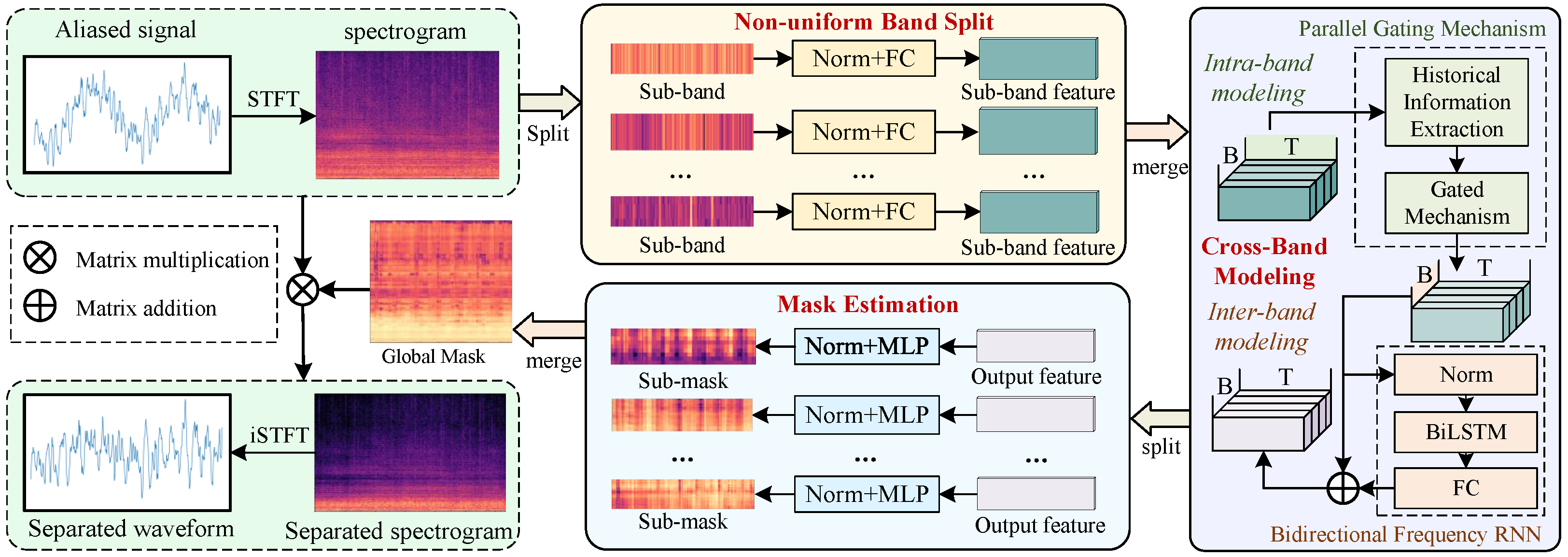
In this section, we present RCBNet in detail, as overviewed in Figure 1. RCBNet first applies Short-Time Fourier Transform (STFT) [37] to the input underwater-aliased signal, obtaining its complex spectrogram. The non-uniform band split module then divides this spectrogram into multiple sub-bands aligned with the harmonic intervals of ship-radiated noise, enabling frequency-specific feature enhancement. These sub-bands are then merged into the cross-band modeling module, which balances intra-band noise suppression and inter-band harmonic consistency during separation. Subsequently, the mask estimation module re-splits the cross-band-refined features into sub-bands so as to generate time–frequency sub-masks. Finally, these masks are aggregated into a global mask, which is element-wise multiplied with the original spectrogram to reconstruct the separated target source’s spectrogram and waveform. In the following, we will introduce each component in detail.

3.1. Non-Uniform Band Split

Traditional neural networks typically process global spectrograms directly in time–frequency feature extraction. For instance, self-attention mechanisms tend to focus on energy-concentrated regions [38]. However, ship-radiated noise in underwater acoustic signals exhibits unique harmonic structures (fundamental frequencies and integer multiples) with distinct spectral energy distributions across frequency bands. In addition, critical harmonic components predominantly reside in lower-frequency bands despite their relatively weaker energy intensity [39]. Therefore, direct feature extraction from the full spectrogram biases the model’s attention toward regions with higher overall energy, which fails to adapt effectively to the unique characteristics of underwater acoustic signals, limiting feature discriminability.

To address this, we propose a harmonic-aligned non-uniform band split strategy, which creates sub-bands where energy intensities become more homogeneous within each band, so as to capture low-frequency dominant features that characterize underwater acoustic signals.

The aliased signal first undergoes STFT to obtain a complex spectrogram. Specifically, the time-domain signal $x\in {\mathbb{R}}^T$ is divided into Z overlapping frames with length N and hop size M. The z-th frame is expressed as follows:

$$x_z\left[n\right]=x[zM+n],0\le n<N,$$

(1)

where n denotes the sample index within a frame. A Hanning window $w\left[n\right]$ is then applied to reduce spectral leakage:

$${\tilde{x}}_z\left[n\right]=x_z\left[n\right]·w\left[n\right],w\left[n\right]=0.5\left(1-cos\left({\displaystyle \frac{2\pi n}{N-1}}\right)\right).$$

(2)

The windowed signal undergoes FFT to generate the complex spectrogram $S\in {\mathbb{C}}^{Z\times F}$:

$$S_z\left[k\right]=\sum _{n=0}^{N-1}{\tilde{x}}_z\left[n\right]e^{-j2\pi kn/N},0\le k<F,$$

(3)

where k represents the frequency bin index.

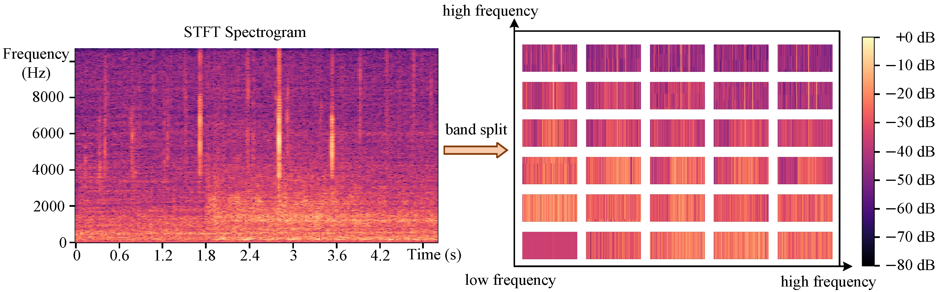
The non-uniform band split strategy adaptively partitions the spectrogram based on the harmonic characteristics of ship noise. The full frequency range $\mathcal{F}=[0,f_{\max }]$ is divided into B sub-bands ${\left\{{\mathcal{F}}_b\right\}}_{b=1}^B$ with progressively increasing bandwidths: 0–1 kHz bands use 100 Hz resolution to capture dense harmonics; 1–4 kHz bands employ 250 Hz intervals; 4–8 kHz and 8–11 kHz regions use 500 Hz and 1 kHz bandwidths, respectively; and frequencies above 11 kHz are consolidated into a single sub-band.

This hierarchical partitioning ensures that energy distributions within each sub-band exhibit similar intensity levels, particularly in the low-frequency regions where ship noise harmonics dominate. The b-th sub-band spectrogram $S_b\in {\mathbb{C}}^{Z\times \Delta f_b}$ spans the frequency range ${\mathcal{F}}_b=[f_b^{\mathrm{low}},f_b^{\mathrm{high}}]$ with bandwidth $\Delta f_b=f_b^{\mathrm{high}}-f_b^{\mathrm{low}}$.

As shown in Figure 2, this decomposition creates sub-bands where energy intensities become more homogeneous within each band, particularly enhancing the model’s capability to capture low-frequency dominant features that characterize underwater acoustic signals.

Each sub-band undergoes layer normalization along the time and frequency axes to mitigate amplitude variations:

$${\widehat{S}}_b=\mathrm{LayerNorm}\left(S_b\right).$$

(4)

A dedicated fully connected layer then projects variable-length sub-band spectrograms into fixed-dimensional features $E_b\in {\mathbb{R}}^d$:

$$E_b={\mathrm{FC}}_b\left({\widehat{S}}_b\right),1\le b\le B,$$

(5)

3.2. Cross-Band Modeling

On the basis of the obtained sub-band features E, we propose a cross-band modeling module that addresses two complementary objectives: (1) suppressing non-stationary noise through intra-band modeling, and (2) maintaining harmonic consistency via inter-band modeling. On one hand, most neural networks rely on MSE-based methods, while the non-stationary noise characteristics in underwater environments limit their ability to capture time–frequency features. To enhance the robustness, motivated by the latest RNN research [40], we apply the parallel gating mechanism (PGM) within intra-band modeling, which improves information extraction under non-stationary noise. On the other hand, as different sub-bands in the same spectrogram frame inherently exhibit frequency correlations between harmonics, we design a bidirectional-frequency RNN within inter-band modeling so as to capture the global harmonic structure.

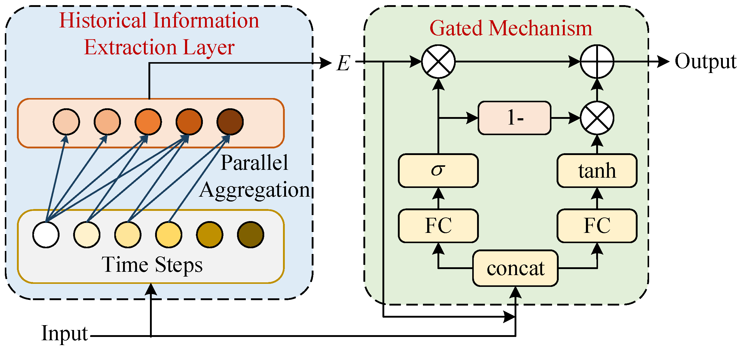
As illustrated in Figure 3, for intra-band modeling, PGM consists of a Historical Information Extraction (HIE) layer and a gating mechanism. HIE employs causal convolution to aggregate contextual dependencies parallelly, while the gating mechanism performs feature fusion through dynamic weighting.

Specifically, given input features $E_b^{(1:T)}=[E_b^{\left(1\right)},\cdots ,E_b^{\left(T\right)}]$ where T denotes time steps, the HIE layer first aggregates all the relevant historical information at each time step through parallel sliding operations along the sequence length dimension:

$${\tilde{E}}_b^{\left(t\right)}=\sum _{i=0}^{L-1}{W}_{\mathrm{HIE}}^{\left(i\right)}·\mathrm{Padding}\left(E_b^{(t-i)}\right),$$

(6)

where $W_{\mathrm{HIE}}\in {\mathbb{R}}^{d\times L}$ denotes learnable convolution kernels with receptive field L, and zero-padding maintains the temporal resolution. The gating mechanism then performs dynamic feature enhancement. First, the sigmoid-activated gate $G_b^{\left(t\right)}\in {[0,1]}^d$ learns frequency-specific thresholds to suppress non-stationary noise components. It computes activation weights by concatenating contextual features ${\tilde{E}}_b^{\left(t\right)}$ (from the HIE layer) and original features $E_b^{\left(t\right)}$, followed by linear projection $W_g$:

$$\begin{array}{cc}\hfill G_b^{\left(t\right)}& =\sigma (W_g·[{\tilde{E}}_b^{\left(t\right)};E_b^{\left(t\right)}]).\hfill \end{array}$$

(7)

Parallelly, the tanh-activated candidate features $C_b^{\left(t\right)}\in {[-1,1]}^d$ are computed using a separate projection matrix $W_c$:

$$\begin{array}{cc}\hfill C_b^{\left(t\right)}& =tanh(W_c·[{\tilde{E}}_b^{\left(t\right)};E_b^{\left(t\right)}]),\hfill \end{array}$$

(8)

where the shared projection dimensions ($W_g,W_c\in {\mathbb{R}}^{2d\times d}$) maintain low computational overhead while enabling cross-band interactions. The final output $H_b^{\left(t\right)}$ combines the gated candidate features and original features through element-wise interpolation:

$$\begin{array}{cc}\hfill H_b^{\left(t\right)}& =G_b^{\left(t\right)}\odot C_b^{\left(t\right)}+(1-G_b^{\left(t\right)})\odot E_b^{\left(t\right)},\hfill \end{array}$$

(9)

where $(1-G_b^{\left(t\right)})\odot E_b^{\left(t\right)}$ prevents over-suppression of critical harmonics.

For inter-band modeling, at each time step t, the normalized features $\{H_1^{\left(t\right)},\cdots ,H_B^{\left(t\right)}\}$ from all sub-bands undergo layer normalization and bidirectional LSTM processing:

$$\begin{array}{cc}\hfill {\widehat{H}}_b^{\left(t\right)}& =\mathrm{LayerNorm}\left(H_b^{\left(t\right)}\right),\hfill \\ \hfill {\overrightarrow{F}}_b^{\left(t\right)}& ={\mathrm{LSTM}}_{\mathrm{forward}}({\widehat{H}}_b^{\left(t\right)},{\overrightarrow{F}}_{b-1}^{\left(t\right)}),\hfill \\ \hfill {\overleftarrow{F}}_b^{\left(t\right)}& ={\mathrm{LSTM}}_{\mathrm{backward}}({\widehat{H}}_b^{\left(t\right)},{\overleftarrow{F}}_{b+1}^{\left(t\right)}),\hfill \\ \hfill F_b^{\left(t\right)}& =W_{\mathrm{FC}}·[{\overrightarrow{F}}_b^{\left(t\right)};{\overleftarrow{F}}_b^{\left(t\right)}]+H_b^{\left(t\right)},\hfill \end{array}$$

(10)

where the residual connection preserves the original harmonic information. Stacking multiple RNN layers progressively strengthens global frequency interaction, enforcing structural constraints between harmonic components.

The final cross-band features $F_b$ integrate both the temporal denoising capability from the PGM and harmonic coherence from the frequency RNN.

3.3. Mask Estimation

To adapt to characteristics across frequency bands, the mask estimation module implements sub-band specialized processing through dedicated pathways. The cross-band refined features $F_b\in {\mathbb{R}}^d$ are first re-split according to the original non-uniform band configuration. Each sub-band feature undergoes independent processing through a three-layer MLP with residual connections:

$$\begin{array}{cc}\hfill {\tilde{F}}_b& =\mathrm{LayerNorm}\left(F_b\right)\hfill \\ \hfill M_b& =W_2\left(\mathrm{GELU}\left(W_1{\tilde{F}}_b\right)\right)+{\tilde{F}}_b,\hfill \end{array}$$

(11)

where $\mathrm{GELU}(·)$ represents the Gaussian Error Linear Unit [41], and $W_1\in {\mathbb{R}}^{d\times 4d}$ and $W_2\in {\mathbb{R}}^{4d\times \Delta f_b}$ form frequency-specific projection matrices. The sub-band masks ${\left\{M_b\right\}}_{b=1}^B$ are concatenated along the frequency axis to construct the global mask $M_{\mathrm{global}}\in {\mathbb{R}}^{Z\times F}$. Target spectrogram reconstruction is achieved through element-wise multiplication with the mixture spectrogram S:

$$\widehat{S}=M_{\mathrm{global}}\odot S.$$

(12)

Time-domain waveform reconstruction is performed via inverse STFT [42]:

$$\widehat{s}=\mathrm{iSTFT}\left(\widehat{S}\right).$$

(13)

Finally, the training objective combines spectral and waveform reconstruction losses. Spectral loss measures the fidelity of reconstructed complex spectrograms by computing the mean absolute errors (MAEs) [43] between the real and imaginary components of the target (S) and estimated ($\widehat{S}$) spectrograms:

$${\mathcal{L}}_{\mathrm{freq}}={\displaystyle \frac{1}{ZF}}\sum _{z=1}^Z\sum _{k=1}^F\left(|\Re \left(S_{z,k}\right)-\Re ({\widehat{S}}_{z,k})|+|\Im \left(S_{z,k}\right)-\Im ({\widehat{S}}_{z,k})|\right),$$

(14)

where Z denotes the total time frames, F the frequency bins, and $\Re (·)$ and $\Im (·)$ the extract real/imaginary parts, respectively. Simultaneously, temporal loss enforces sample-wise waveform consistency between original (s) and reconstructed ($\widehat{s}$) signals through the MAE:

$${\mathcal{L}}_{\mathrm{time}}={\displaystyle \frac{1}{T}}\sum _{t=1}^T|s\left(t\right)-\widehat{s}\left(t\right)|,$$

(15)

where T represents the total time samples.

Finally, the total loss combines both losses:

$${\mathcal{L}}_{\mathrm{total}}={\mathcal{L}}_{\mathrm{freq}}+\lambda {\mathcal{L}}_{\mathrm{time}},$$

(16)

where $\lambda$ (empirically set to 1.0) balances the spectral–temporal trade-offs.

4. Experiments and Results

In this section, we present the experiments and results of RCBNet. First, we introduce the dataset, baselines, evaluation metrics, and implementation details and then present the experimental results.

4.1. Dataset and Preprocessing

We adopt the ShipsEar dataset [44] for model training and evaluation, which comprises 90 audio recordings sampled at 52,734 Hz with durations ranging from 15 s to 15 min. These recordings include 11 types of ship engine noises and natural environmental sounds, categorized into five classes.

To construct challenging source separation scenarios, we select passenger ships and motorboats as target sources based on two classes. On the one hand, their overlapping time–frequency distributions approximate real-world underwater acoustic-aliasing conditions. On the other hand, sufficient sample quantities (686 passenger ship clips and 159 motorboat clips after 5 s segmentation) ensure model generalization. The original recordings are segmented into 5 s clips and downsampled to 22,050 Hz.

Subsequently, in order to simulate realistic underwater propagation effects, we implement physical augmentation preprocessing as follows. First, we randomly pair passenger ship and motorboat clips, scaling motorboat power $P_{\mathrm{mb}}$ to match passenger ship power $P_{\mathrm{ps}}$:

$$P_{\mathrm{mb}}^{\prime }=P_{\mathrm{mb}}\times {\displaystyle \frac{P_{\mathrm{ps}}}{\mathbb{E}\left[P_{\mathrm{mb}}\right]}}.$$

(17)

Next, we model propagation loss by combining spherical spreading and frequency-dependent absorption using Thorp’s formula [45]:

$$L(f,r)=20{log}_{10}\left(r\right)+{\displaystyle \frac{r}{1000}}\left({\displaystyle \frac{0.11f^2}{1+f^2}}+{\displaystyle \frac{44f^2}{4100+f^2}}+2.75\times {10}^{-4}{f}^2+0.003\right).$$

(18)

Moreover, we simulate three propagation paths (direct, surface-reflected, and bottom-reflected) with the respective delays ${\tau }_i$ and frequency responses $H_i\left(f\right)$:

$$x_{\mathrm{mb}}\left(t\right)=\sum _{i=1}^3{H}_i\left(f\right)x(t-{\tau }_i).$$

(19)

Finally, we combine augmented signals to create 2-mix samples:

$$x_{\mathrm{mix}}=x_{\mathrm{ps}}+x_{\mathrm{mb}}.$$

(20)

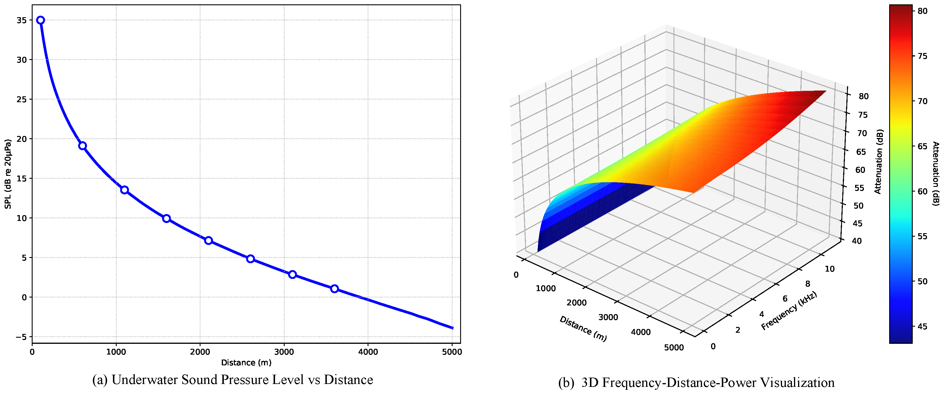
Figure 4 illustrates the physical augmentation processing. Figure 4a demonstrates the reduction in the sound pressure level (SPL) with increasing propagation distance, while Figure 4b illustrates the frequency-dependent attenuation and aliasing phenomena affecting different spectral components during propagation.

For computational tractability, we establish a 2000 m propagation distance and implement multipath propagation simulation. The final dataset is split into training (70%), validation (10%), and test (20%) sets.

Note that all the results in this work are derived from preprocessed data. While omitting this preprocessing step may superficially improve certain performance metrics, such results are obtained under overly idealized conditions and may not adequately reflect the complexities encountered in real-world deployment scenarios. Consequently, we exclusively used physically simulated data for both training and testing to ensure a more accurate and application-relevant evaluation of our method.

4.2. Baselines

Following [12], we first apply advanced comparisons using three fundamental deep learning architectures for underwater BSS, including RNN [46], transformer [38], and U-Net [33] models. Additionally, we include recent state-of-the-art underwater BSS approaches, including IAM [9] and Recurrent Attention Neural Network (RANN) [12]. IAM employs deep bidirectional long short-term memory (BiLSTM) recurrent networks to process STFT magnitude features, while RANN implements an end-to-end architecture combining attention mechanisms with bidirectional LSTM modules.

Table 1. Parameter counts between the baseline models and the proposed RCBNet.

Model	Parameters
RNN	0.3 M
Transformer	24 K
U-Net	3.4 M
RANN	2.1 M
IAM	49.4 M
RCBNet	7.3 M

compares the parameter counts between the baseline models and the proposed RCBNet.

4.3. Evaluation Metrics

The experimental evaluation employs the Signal-to-Distortion Ratio (SDR) [47]. As the standard metric for BSS, the SDR evaluates both separation fidelity through interference suppression and system robustness against non-stationary noise, which is particularly suitable for performance validation in underwater acoustic scenarios characterized by complex mixing mechanisms. The SDR is defined as follows:

$$\mathrm{SDR}=10{log}_{10}\left({\displaystyle \frac{{\parallel \alpha \mathbf{s}\parallel }^2}{\parallel \widehat{\mathbf{s}}{-\alpha \mathbf{s}\parallel }^2}}\right),$$

(21)

where $\mathbf{s}$ denotes the original source signal; $\widehat{\mathbf{s}}$ represents the separated signal. $\alpha$ represents the optimal scaling factor calculated through least-squares projection:

$$\alpha ={\displaystyle \frac{{\mathbf{s}}^{\top }\widehat{\mathbf{s}}}{{\parallel \mathbf{s}\parallel }^2}}.$$

(22)

where the numerator ${\parallel \alpha \mathbf{s}\parallel }^2$ captures the preserved target signal energy after optimal scaling, while the denominator $\parallel \widehat{\mathbf{s}}{-\alpha \mathbf{s}\parallel }^2$ aggregates all the distortion components, including environmental noise residuals and algorithmic artifacts. Higher SDR values indicate superior separation performance with precise signal reconstruction and minimal distortion. The SDR has been widely adopted in BSS benchmarks and is well suited for underwater environments where complex propagation paths and noise are common.

In addition, we utilize the MSE as another metric, which quantifies the average squared discrepancy between model predictions and ground truth values. Lower MSE values indicate superior prediction accuracy, while a higher MSE reflects greater prediction errors. Formally,

$$\mathrm{MSE}={\displaystyle \frac{1}{N}}\sum _{i=1}^N{(y_i-{\widehat{y}}_i)}^2$$

(23)

where $y_i$ and ${\widehat{y}}_i$ denote the true value and predicted value of the i-th sample, respectively, with N being the total number of samples.

4.4. Implementation Details

All the experiments are conducted on a single NVIDIA RTX 3090 GPU with an Intel Core i7-9750H CPU. The model is optimized using Adam [48] with the initial learning rate $\eta ={10}^{-3}$ decaying by 0.98 every two epochs. Training employs early stopping that terminated optimization when no validation loss improvement occurred for 10 consecutive epochs. The parameter update rule follows:

$${\theta }_t={\theta }_{t-1}-\eta {\displaystyle \frac{{\widehat{m}}_t}{\sqrt{{\widehat{v}}_t}+ϵ}}$$

(24)

where ${\widehat{m}}_t$ and ${\widehat{v}}_t$ denote bias-corrected first/second moment estimates, $ϵ={10}^{-8}$ prevents division by zero, and $\eta$ controls the update magnitude. The default exponential decay rates ${\beta }_1=0.9$ and ${\beta }_2=0.999$ govern the moving averages of the gradients and squared gradients, respectively.

The model occupies 121.21 MB of storage, demonstrates an average inference latency of 0.342 s per sample with the batch size set to 8, and reaches a peak GPU memory consumption of 6516.14 MB during execution.

4.5. Separation Results

In the following, we present the BSS capabilities of RCBNet through the spectrum and waveform separation results, respectively.

4.5.1. Spectral Separation Results

Figure 5 illustrates the spectral separation performance. The original passenger ship spectrogram (Figure 5a) demonstrates characteristic low-frequency dominance between 0 and 2500 Hz, exhibiting a stable temporal energy distribution indicative of consistent mechanical vibrations from engine operations. This contrasts with the motorboat spectrogram (Figure 5b), which spans a broader frequency range up to 5000 Hz with pronounced mid/high-frequency components showing temporal variability.

The aliased signal spectrogram (Figure 5c) reveals the spectral superposition where motorboat signatures dominate across both low and high frequencies. The low-frequency bands (0–2500 Hz) exhibit energy patterns closely resembling the motorboat profile, while frequencies above 5000 Hz retain the amount of the motorboat’s spectral characteristics. This masking effect substantially obscures the passenger ship’s periodic features, particularly in the mid-frequency ranges where energy distributions demonstrate complex interference patterns.

Notably, the separation results (Figure 5d) successfully recover passenger ship signatures by reconstructing the low-frequency components that match the spectral morphology of the original passenger ship features. In addition, the separation output demonstrates effective suppression of motorboat interference through frequency-selective processing. Significant energy attenuation in the mid/high-frequency regions (2500–5000 Hz) specifically targets propeller cavitation noise and hydrodynamic wake signatures characteristic of motorboat operation. Simultaneously, the algorithm preserves temporal coherence in low-frequency bands (0–2500 Hz), reconstructing the sustained vibrational patterns inherent to passenger ship engine dynamics.

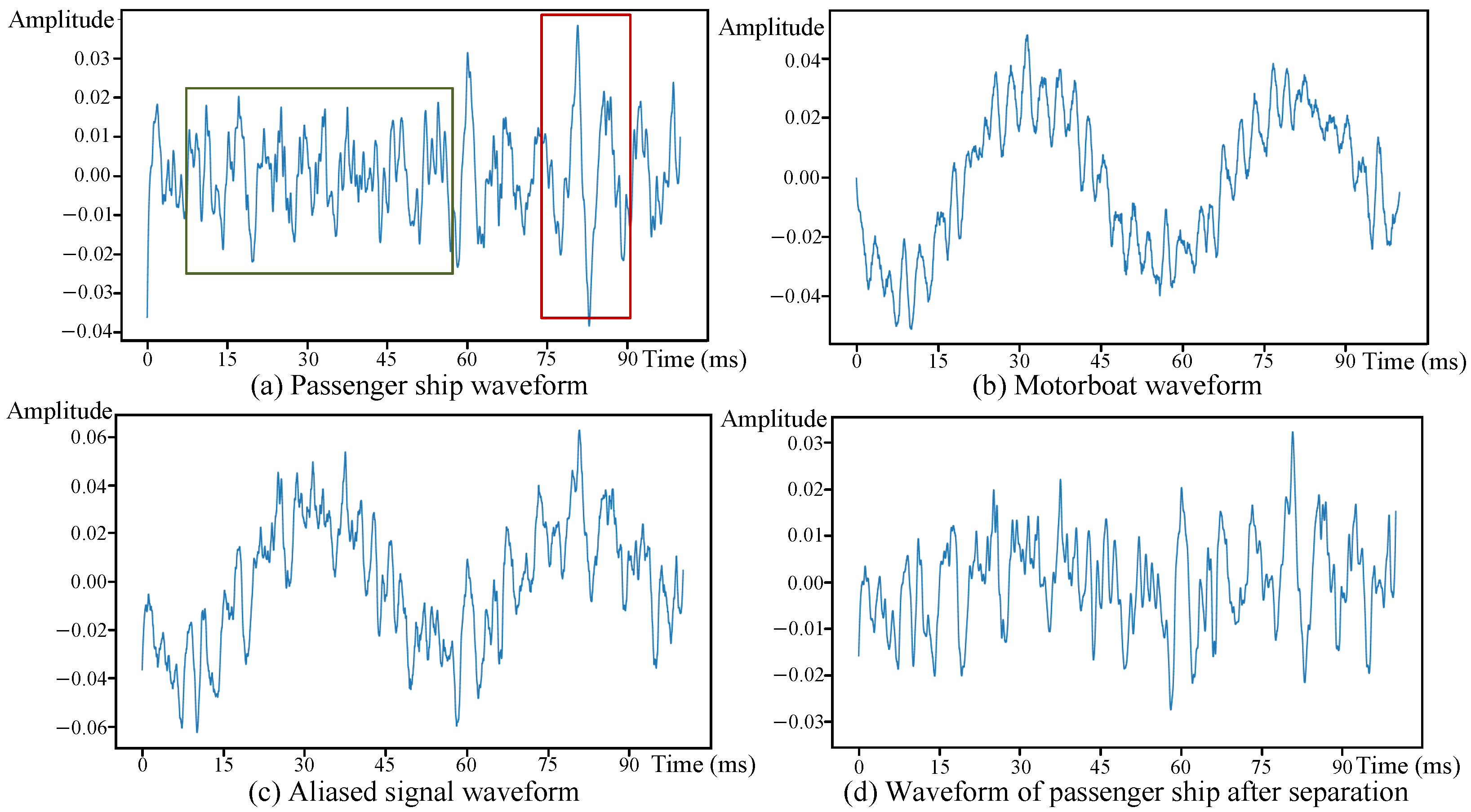
4.5.2. Waveform Separation Results

Figure 6 illustrates the waveform separation performance. The original passenger ship waveform (Figure 6a) exhibits complex temporal fluctuations, particularly showing intense amplitude variations between 0.015 and 0.060 s corresponding to mechanical vibrations from engine operations. Subsequently, this is followed by damped oscillatory patterns at 0.075–0.090 s indicative of secondary mechanical or environmental interactions. In contrast, the motorboat waveform (Figure 6b) displays greater amplitude stability with marginally higher peak values, reflecting consistent mechanical vibrations from its propulsion system.

The aliased signal waveform (Figure 6c) reveals the dominance of the motorboat characteristics, particularly through sustained amplitude levels that obscure the passenger ship’s transient fluctuations. Critical features of the passenger ship between 0.015 and 0.060 s are attenuated in the mixed signal, while motorboat signatures maintain their original amplitude.

The separation results (Figure 6d) demonstrate effective recovery of passenger ship signatures. As a result, (1) RCBNet successfully reconstructs transient high-amplitude fluctuations between 0.015 and 0.060 s and preserves oscillatory patterns near 0.080 s. (2) The processed waveform reduces motorboat-induced amplitude dominance while restoring temporal features closely matching the original passenger ship profile. The results demonstrate RCBNet’s capability to disentangle overlapping transient patterns despite significant amplitude disparities in mixed signals. Such results demonstrate the strong separation capability of RCBNet.

4.6. Quantitative Comparison

We present quantitative comparison experiments between RCBNet and the state-of-the-art models using established evaluation metrics.

Table 2. Separation performance comparison under SDR (dB) and MSE metrics.

Model	SDR (dB)	MSE
U-Net	−4.453	0.053
Transformer	−2.947	0.037
IAM	4.360	0.004
RNN	4.495	0.007
RANN	4.684	0.006
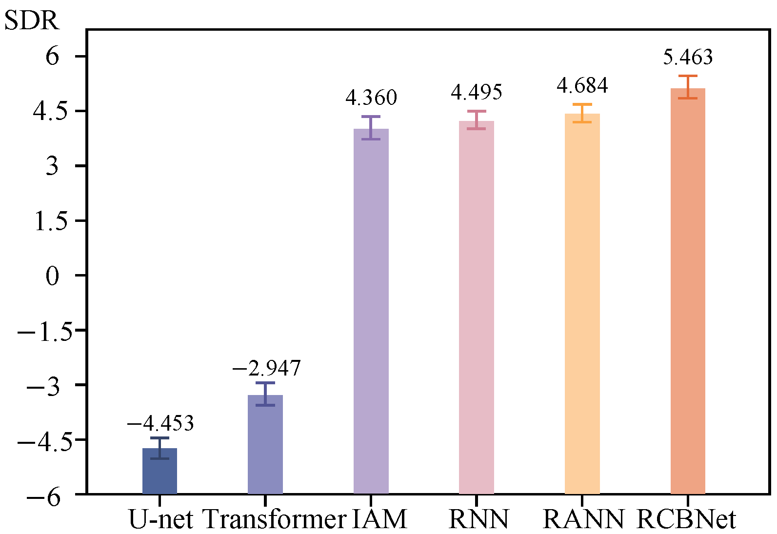
RCBNet	5.463	0.002

presents the separation performance across different models under SDR and MSE metrics. Furthermore, Figure 7 illustrates the SDR variation results under different random seeds, where the upper and lower bounds represent the maximum and minimum values observed across experimental trials, respectively.

The following can be observed: (1) As shown in Table 2, RCBNet achieves superior separation performance with an SDR of 5.463 dB, outperforming other advanced methods by 0.779 dB. Figure 7 presents RCBNet’s enhanced stability against random initialization. This demonstrates that our sub-band modules effectively focus on distinct frequency bands while the cross-band modeling strengthens time–frequency discriminability. (2) Both U-Net and transformer exhibit unsatisfactory performance (SDR < 3.3 dB), aligning with our hypothesis that their general-purpose architectures struggle with underwater non-stationary noise. (3) RNN-based approaches (IAM/RANN) show moderate improvements through Bi-LSTM temporal modeling (SDR: 4.360–4.684 dB). However, their higher MSE scores (>0.005) reveal inadequate signal reconstruction and potential overfitting risks. (4) Notably, RCBNet achieves a breakthrough MSE of 0.002, which demonstrates RCBNet’s exceptional signal reconstruction fidelity through detailed waveform recovery.

In conclusion, such results demonstrate that RCBNet exhibits superior separation capability and outperforms other advanced methods.

5. Discussion

In this section, we discuss the anti-noise robustness, inter-band modeling effectiveness, the impact of the different band-splitting strategies, and the ablation study of RCBNet.

5.1. Anti-Noise Discussion

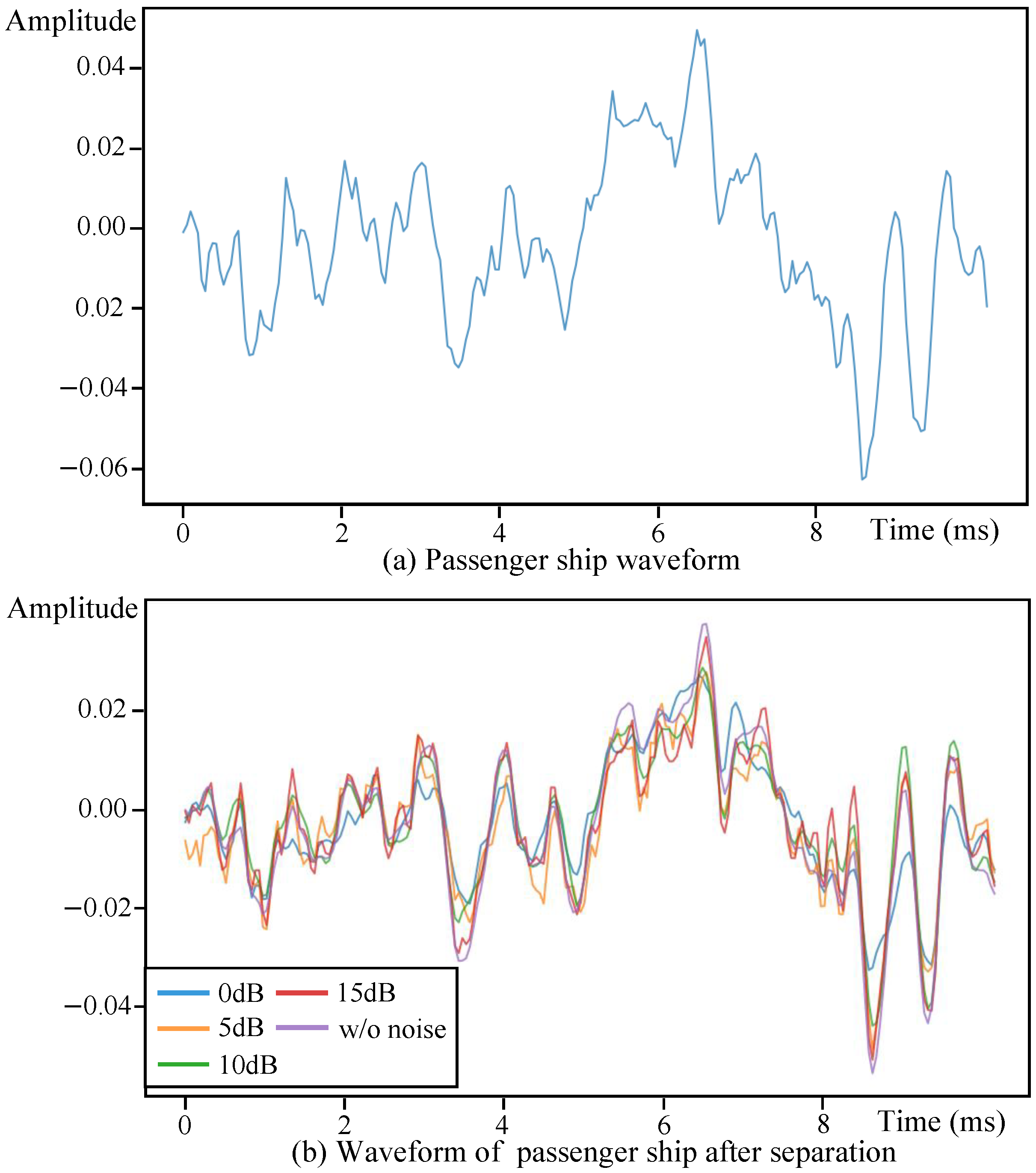
To systematically evaluate model robustness, we introduce additive Gaussian white noise with varying signal-to-noise ratio (SNR) levels to both the IAM and RCBNet architectures. Specifically, we inject white noise at SNR intervals of 0 dB, 5 dB, 10 dB, and 15 dB and use a noiseless condition as the baseline reference. SNR indicates the energy ratio of noise to signal. The lower the value, the stronger the noise.

Table 3. Noise robustness experimental results (SDR in dB).

Noise Level (SNR)	RCBNet	IAM
0 dB	4.366	2.779
5 dB	4.879	3.537
10 dB	5.308	3.942
15 dB	5.379	3.980
w/o noise	5.463	4.360

presents the noise robustness evaluation results, where the noise level represents the signal-to-noise ratio between the target sounds and background interference. Both RCBNet and IAM exhibit progressive performance improvements as the SNR increases from 0 dB to noiseless conditions, demonstrating their inherent noise-resistant capabilities. Notably, RCBNet achieves an SDR of 4.366 under 0 dB strong noise conditions, surpassing IAM’s noiseless performance of 4.360 SDR. This highlights RCBNet’s exceptional effectiveness in high-noise environments and its superior capacity for feature modeling and source separation even under extreme acoustic interference.

A further quantitative analysis reveals distinct performance degradation patterns: RCBNet shows only a 20.1% relative SDR reduction from noiseless to 0 dB conditions, compared to IAM’s substantial 36.3% degradation. This evidence demonstrates RCBNet’s enhanced noise robustness through its advanced spectral modeling strategy and stable feature extraction mechanism. The comparative results clearly indicate RCBNet’s practical superiority for real-world underwater source separation tasks, particularly in challenging acoustic environments where IAM demonstrates limited robustness and notable performance deterioration under intense noise conditions.

Figure 8b provides waveform-level insights. As in the figure, RCBNet demonstrates progressive waveform reconstruction improvement with an increasing SNR. Under 0 dB conditions, the model successfully preserves the passenger ship’s primary waveform structure despite strong interference, exhibiting minor peak deviations at 0.003 s and a slightly reduced amplitude after 0.008 s while maintaining the overall temporal characteristics. When the SNR increases to 5 dB, the reconstructed waveform shows enhanced contour definition with reduced motorboat signal similarity in the initial segments and improved amplitude accuracy beyond 0.008 s. At a 10 dB SNR, the reconstruction achieves near-perfect shape alignment with the original signal, displaying only minimal peak overestimation near 0.008 s. The 15 dB condition yields almost complete waveform recovery, with merely negligible fluctuations at the 0.003 s peak position, confirming the model’s exceptional stability in moderate-noise environments.

It is worth noting that while RCBNet achieves a satisfactory MSE, slight disparities persist between the shapes of its reconstructed waveform and the original waveform. We attribute this to the model’s deliberate prioritization of preserving harmonic structures while suppressing transient artifacts in high-noise regions, thereby enhancing perceptual signal fidelity.

In general, such results demonstrate the robustness of our proposed RCBNet.

5.2. Inter-Band Modeling Discussion

To evaluate the contribution of the frequency-domain RNNs for inter-band modeling within RCBNet, we compare it against alternative architectures, including attention mechanisms [38], GCN [49], and frequency-convolutional layers.

Table 4. Inter-band modeling discussion experimental results.

Model	SDR
attention mechanisms	4.982
GCN	5.220
frequency-convolutional layers	5.308
RCBNet	5.463

presents the inter-band modeling comparative experimental results for the different modules. The following can be observed: (1) The full RCBNet model achieves the best source separation performance, with an SDR of 5.463 dB, which demonstrates the effectiveness of its bidirectional temporal modeling and module integration. (2) Replacing the RNN with a frequency-convolutional block results in a slight decline in the SDR to 5.308 dB, which suggests that while modeling frequency-local patterns is beneficial, the approach lacks sufficient temporal context modeling. (3) The GCN-based variant yields a performance of 5.220 dB, which indicates that graph-based feature propagation introduces useful structural information; however, its capability remains limited by weak temporal modeling. (4) The self-attention-based version achieves an SDR of 4.982 dB. This suggests that although attention mechanisms can capture long-range dependencies, their lack of inductive bias towards temporal continuity may impair performance in the dynamic, non-stationary underwater environment. These results demonstrate the advantages of using frequency-domain RNNs for inter-band modeling. They further highlight the necessity of modeling temporal consistency for effective underwater source separation.

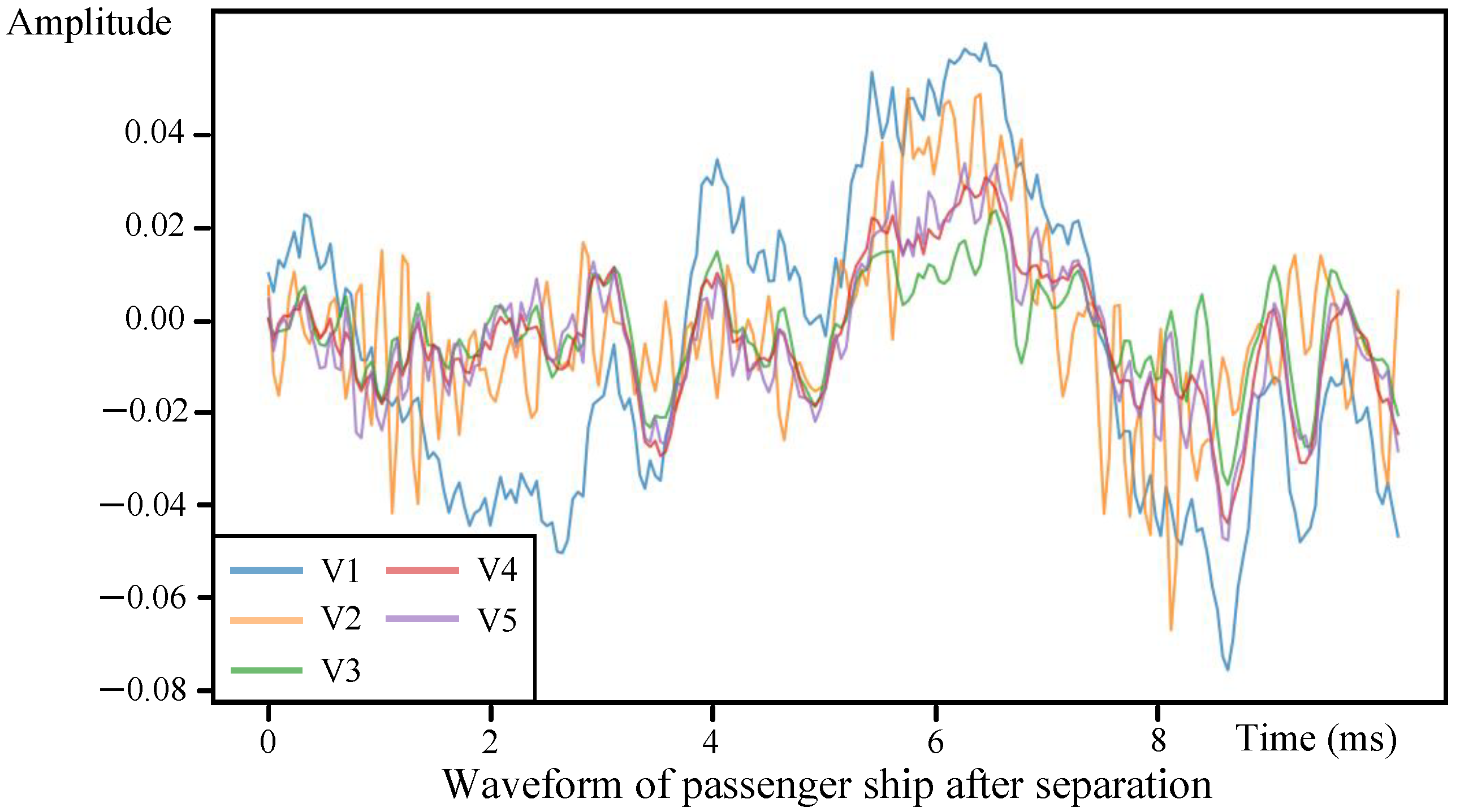
5.3. Impact of Band-Splitting Strategies

To evaluate the separation performance of different band-splitting strategies, we compare five band-splitting approaches in

Table 5. Separation performance under different band-splitting strategies.

No.	Band-Splitting Strategy	SDR (dB)
V1	5 kHz Uniform	4.770
V2	3 kHz Uniform	5.222
V3	1 kHz Uniform	5.355
V4	Tiered Non-uniform	5.383
V5	Refined Non-uniform	5.463

. Strategy V1 utilizes uniform 5 kHz bands, V2 employs 3 kHz uniform bands, V3 applies 1 kHz uniform bands, V4 implements tiered splitting (250 Hz below 4 kHz, 500 Hz from 4–8 kHz, and 1 kHz from 8–11 kHz), and V5 (our non-uniform band-splitting) further refines this with 100 Hz bands below 1 kHz.

It can be observed from Table 5 that the progressive SDR improvements from 4.770 dB (V1) to 5.463 dB (V5) demonstrate the non-uniform band-splitting’s superiority in handling underwater acoustic characteristics.

Figure 9 provides waveform-level insights. The coarsest band-splitting (V1) shows significant waveform distortion with incomplete transient feature recovery. V2’s moderate splitting reduces but does not eliminate oscillatory artifacts, while V3’s finer uniform bands demonstrate improved temporal alignment at the cost of missing characteristic low-frequency components. The non-uniform strategies (V4/V5) enhanced the preservation of the engine harmonic structures through low-frequency splitting. In addition, the reconstruction presents the closest visual correspondence to the original signals, which demonstrates inherent advantages in underwater acoustic separation.

In conclusion, such experiments demonstrate that non-uniform band-splitting better resolves the fundamental challenge from wideband interference in underwater environments.

5.4. Ablation Study

In the following, we discuss the ablation study to evaluate the contributions of the key components in RCBNet.

Table 6. Ablation study results of RCBNet components, where “w/o” represents RCBNet without certain modulesThe following highlights are the same. “NBS” represents non-uniform band split module, and “CBM” represents cross-band modeling module.

Group	Model Configuration	SDR (dB)
1	w/o NBS and CBM	4.721
2	w/o NBS	5.015
3	w/o CBM	4.779
4	full RCBNet	5.463
5	w/o gating mechanism	4.932

presents the ablation study results. The following can be observed: (1) Group 2 achieves a 5.015 dB SDR by retaining band-splitting while removing cross-band modeling, showing a 6.2% improvement over Group 1. This demonstrates the fundamental importance of frequency band decomposition. Similarly, Group 4 (full model) outperforms Group 3 by 14.3%, demonstrating the critical role of cross-band interaction modeling. (2) The marginal SDR improvement in Group 3 (+1.2% over Group 1) suggests limited benefits from intra-band modeling alone. The 8.9% SDR boost in Group 4 compared to Group 2 demonstrates the necessity of cross-band feature modeling. (3) The optimal performance of Group 4 demonstrates synergistic cooperation between non-uniform band-splitting and cross-band modeling modules. (4) In Group 5, the gating mechanism is removed, while all the other components remain identical to Group 4. This results in an SDR performance drop to 4.932 dB, representing a 9.7% degradation compared to the full model. These findings underscore the gating mechanism’s critical role in dynamically regulating information flow and suppressing non-stationary noise components.

Figure 10 provides waveform-level insights. Group 1 shows a significant deviation from the original signal. Group 2 recovers basic waveform contours but introduces overshoot during the rising edge near 0.004 s, revealing localized temporal estimation errors that cross-band constraints could mitigate. Group 3 achieves high temporal alignment with the precise reconstruction of subtle fluctuations at 0.0025 s and 0.0065 s, demonstrating the intra-band modules’ capacity for local temporal coherence preservation. Group 4 produces near-perfect waveform matching with smoother slope transitions and enhanced structural continuity. Compared with Group 4, the waveform of Group 5 changes more dramatically, which indirectly proves the contribution of the gating mechanism to suppressing non-stationary noise.

In general, the ablative results demonstrate the effectiveness of our designed modules.

6. Conclusions and Future Work

In this work, we propose a novel Robust Cross-Band Network (RCBNet) for underwater BSS to overcome limited feature discrimination and inadequate robustness against non-stationary noise challenges. We first propose a non-uniform band split strategy to decompose mixed signals. Next, we apply a parallel gating mechanism for intra-band modeling to enhance robustness. Subsequently, we design a bidirectional-frequency RNN for inter-band modeling to capture global dependencies. Experimental results demonstrate that RCBNet outperforms the advanced model and achieves a 0.779 dB improvement in the SDR.

In the future, it is worthwhile to study how to further improve the adaptability of deep learning-based BSS models in underwater scenarios and how to reconstruct waveforms under unforeseen complexities and at finer levels of detail. In addition, the integration of reinforcement learning techniques into the RCBNet framework is worth exploring.

References

- Mansour, A.; Benchekroun, N.; Gervaise, C. Blind separation of underwater acoustic signals. In Proceedings of the Independent Component Analysis and Blind Signal Separation: 6th International Conference, ICA 2006, Charleston, SC, USA, 5–8 March 2006; Proceedings 6. Springer: Berlin/Heidelberg, Germany, 2006; pp. 181–188. [Google Scholar]
- Yaman, O.; Tuncer, T.; Tasar, B. DES-Pat: A novel DES pattern-based propeller recognition method using underwater acoustical sounds. Appl. Acoust. 2021, 175, 107859. [Google Scholar] [CrossRef]
- Li, S.; Yu, Z.; Wang, P.; Sun, G.; Wang, J. Blind source separation algorithm for noisy hydroacoustic signals based on decoupled convolutional neural networks. Ocean Eng. 2024, 308, 118188. [Google Scholar] [CrossRef]
- Zhang, X.; Zhang, A.; Fang, J.; Yang, S. Study on blind separation of underwater acoustic signals. In Proceedings of the WCC 2000-ICSP 2000, 2000 5th International Conference on Signal Processing Proceedings, 16th World Computer Congress 2000, Beijing, China, 21–25 August 2000; Volume 3, pp. 1802–1805. [Google Scholar]
- Comon, P. Independent component analysis, a new concept? Signal Process. 1994, 36, 287–314. [Google Scholar] [CrossRef]
- Bofill, P.; Zibulevsky, M. Underdetermined blind source separation using sparse representations. Signal Process. 2001, 81, 2353–2362. [Google Scholar] [CrossRef]
- Seung, D.; Lee, L. Algorithms for non-negative matrix factorization. Adv. Neural Inf. Process. Syst. 2001, 13, 3. [Google Scholar]
- Shijie, T.; Hang, C. Blind source separation of underwater acoustic signal by use of negentropy-based fast ICA algorithm. In Proceedings of the 2015 IEEE International Conference on Computational Intelligence & Communication Technology, Ghaziabad, India, 13–14 February 2015; pp. 608–611. [Google Scholar]
- Zhang, W.; Li, X.; Zhou, A.; Ren, K.; Song, J. Underwater acoustic source separation with deep Bi-LSTM networks. In Proceedings of the 2021 4th International Conference on Information Communication and Signal Processing (ICICSP), Shanghai, China, 24–26 September 2021; pp. 254–258. [Google Scholar]
- Xie, Y.; Xie, K.; Xie, S. Underdetermined blind separation of source using lp-norm diversity measures. Neurocomputing 2020, 411, 259–267. [Google Scholar] [CrossRef]
- Xiao, Y.; Zhu, F.; Zhuang, S.; Yang, Y. Blind source separation and deep feature learning network-based identification of multiple electromagnetic radiation sources. IEEE Trans. Instrum. Meas. 2023, 72, 2508813. [Google Scholar] [CrossRef]
- Song, R.; Feng, X.; Wang, J.; Sun, H.; Zhou, M.; Esmaiel, H. Underwater acoustic nonlinear blind ship noise separation using recurrent attention neural networks. Remote Sens. 2024, 16, 653. [Google Scholar] [CrossRef]
- Davies, M.E.; James, C.J. Source separation using single channel ICA. Signal Process. 2007, 87, 1819–1832. [Google Scholar] [CrossRef]
- Tengtrairat, N.; Woo, W.L.; Dlay, S.S.; Gao, B. Online noisy single-channel source separation using adaptive spectrum amplitude estimator and masking. IEEE Trans. Signal Process. 2015, 64, 1881–1895. [Google Scholar] [CrossRef]
- Georgiev, P.; Theis, F.; Cichocki, A. Sparse component analysis and blind source separation of underdetermined mixtures. IEEE Trans. Neural Netw. 2005, 16, 992–996. [Google Scholar] [CrossRef] [PubMed]
- Nikunen, J.; Diment, A.; Virtanen, T. Separation of moving sound sources using multichannel NMF and acoustic tracking. IEEE/ACM Trans. Audio Speech Lang. Process. 2017, 26, 281–295. [Google Scholar] [CrossRef]
- Deville, Y. Sparse component analysis: A general framework for linear and nonlinear blind source separation and mixture identification. In Blind Source Separation: Advances in Theory, Algorithms and Applications; Springer: Berlin/Heidelberg, Germany, 2014; pp. 151–196. [Google Scholar]
- Erdogan, A.T. An information maximization based blind source separation approach for dependent and independent sources. In Proceedings of the ICASSP 2022-2022 IEEE International Conference on Acoustics, Speech and Signal Processing (ICASSP), Singapore, 22–27 May 2022; pp. 4378–4382. [Google Scholar]
- Koundinya, S.; Karmakar, A. Homotopy optimisation based NMF for audio source separation. IET Signal Process. 2018, 12, 1099–1106. [Google Scholar] [CrossRef]
- Ikeshita, R.; Nakatani, T. Independent vector extraction for fast joint blind source separation and dereverberation. IEEE Signal Process. Lett. 2021, 28, 972–976. [Google Scholar] [CrossRef]
- Li, D.; Wu, M.; Yu, L.; Han, J.; Zhang, H. Single-channel blind source separation of underwater acoustic signals using improved NMF and FastICA. Front. Mar. Sci. 2023, 9, 1097003. [Google Scholar] [CrossRef]
- Rahmati, M.; Pandey, P.; Pompili, D. Separation and classification of underwater acoustic sources. In Proceedings of the 2014 Underwater Communications and Networking (UComms), Sestri Levante, Italy, 3–5 September 2014; pp. 1–5. [Google Scholar]
- De Rango, F.; Veltri, F.; Fazio, P. A multipath fading channel model for underwater shallow acoustic communications. In Proceedings of the 2012 IEEE International Conference on Communications (ICC), Ottawa, ON, Canada, 10–15 June 2012; pp. 3811–3815. [Google Scholar]
- Stojanovic, M. On the relationship between capacity and distance in an underwater acoustic communication channel. ACM SIGMOBILE Mob. Comput. Commun. Rev. 2007, 11, 34–43. [Google Scholar] [CrossRef]
- Luo, Y.; Mesgarani, N. Tasnet: Time-domain audio separation network for real-time, single-channel speech separation. In Proceedings of the 2018 IEEE International Conference on Acoustics, Speech and Signal Processing (ICASSP), Calgary, AB, Canada, 15–20 April 2018; pp. 696–700. [Google Scholar]
- Luo, Y.; Mesgarani, N. Conv-tasnet: Surpassing ideal time–frequency magnitude masking for speech separation. IEEE/ACM Trans. Audio Speech Lang. Process. 2019, 27, 1256–1266. [Google Scholar] [CrossRef]
- Luo, Y.; Chen, Z.; Yoshioka, T. Dual-path rnn: Efficient long sequence modeling for time-domain single-channel speech separation. In Proceedings of the ICASSP 2020-2020 IEEE International Conference on Acoustics, Speech and Signal Processing (ICASSP), Barcelona, Spain, 4–8 May 2020; pp. 46–50. [Google Scholar]
- Lam, M.W.; Wang, J.; Su, D.; Yu, D. Effective low-cost time-domain audio separation using globally attentive locally recurrent networks. In Proceedings of the 2021 IEEE Spoken Language Technology Workshop (SLT), Shenzhen, China, 19–22 January 2021; pp. 801–808. [Google Scholar]
- He, J.; Chen, W.; Song, Y. Single channel blind source separation under deep recurrent neural network. Wirel. Pers. Commun. 2020, 115, 1277–1289. [Google Scholar] [CrossRef]
- Chen, J.; Mao, Q.; Liu, D. Dual-path transformer network: Direct context-aware modeling for end-to-end monaural speech separation. arXiv 2020, arXiv:2007.13975. [Google Scholar]
- Herzog, A.; Chetupalli, S.R.; Habets, E.A. Ambisep: Ambisonic-to-ambisonic reverberant speech separation using transformer networks. In Proceedings of the 2022 International Workshop on Acoustic Signal Enhancement (IWAENC), Bamberg, Germany, 5–8 September 2022; pp. 1–5. [Google Scholar]
- Reddy, P.; Wisdom, S.; Greff, K.; Hershey, J.R.; Kipf, T. Audioslots: A slot-centric generative model for audio separation. In Proceedings of the 2023 IEEE International Conference on Acoustics, Speech, and Signal Processing Workshops (ICASSPW), Rhodes Island, Greece, 4–10 June 2023; pp. 1–5. [Google Scholar]
- Wang, J.; Liu, H.; Ying, H.; Qiu, C.; Li, J.; Anwar, M.S. Attention-based neural network for end-to-end music separation. CAAI Trans. Intell. Technol. 2023, 8, 355–363. [Google Scholar] [CrossRef]
- Zhang, Z.; White, P.R. A blind source separation approach for humpback whale song separation. J. Acoust. Soc. Am. 2017, 141, 2705–2714. [Google Scholar] [CrossRef] [PubMed]
- He, Q.; Wang, H.; Zeng, X.; Jin, A. Ship-Radiated Noise Separation in Underwater Acoustic Environments Using a Deep Time-Domain Network. J. Mar. Sci. Eng. 2024, 12, 885. [Google Scholar] [CrossRef]
- Yu, Y.; Fan, J.; Cai, Z. End-to-end underwater acoustic source separation model based on EDBG-GALR. Sci. Rep. 2024, 14, 24748. [Google Scholar] [CrossRef] [PubMed]
- Chikkerur, S.; Cartwright, A.N.; Govindaraju, V. Fingerprint enhancement using STFT analysis. Pattern Recognit. 2007, 40, 198–211. [Google Scholar] [CrossRef]
- Vaswani, A.; Shazeer, N.; Parmar, N.; Uszkoreit, J.; Jones, L.; Gomez, A.N.; Kaiser, Ł.; Polosukhin, I. Attention is all you need. In Proceedings of the 31st Conference on Neural Information Processing Systems (NIPS 2017), Long Beach, CA, USA, 4–9 December 2017. [Google Scholar]
- McKenna, M.F.; Ross, D.; Wiggins, S.M.; Hildebrand, J.A. Underwater radiated noise from modern commercial ships. J. Acoust. Soc. Am. 2012, 131, 92–103. [Google Scholar] [CrossRef]
- Jia, Y.; Lin, Y.; Yu, J.; Wang, S.; Liu, T.; Wan, H. PGN: The RNN’s New Successor is Effective for Long-Range Time Series Forecasting. Adv. Neural Inf. Process. Syst. 2024, 37, 84139–84168. [Google Scholar]
- Hendrycks, D.; Gimpel, K. Gaussian error linear units (gelus). arXiv 2016, arXiv:1606.08415. [Google Scholar]
- Zhivomirov, H. On the development of STFT-analysis and ISTFT-synthesis routines and their practical implementation. TEM J. 2019, 8, 56–64. [Google Scholar] [CrossRef]
- Hodson, T.O. Root mean square error (RMSE) or mean absolute error (MAE): When to use them or not. Geosci. Model Dev. 2022, 15, 5481–5487. [Google Scholar] [CrossRef]
- Santos-Domínguez, D.; Torres-Guijarro, S.; Cardenal-López, A.; Pena-Gimenez, A. ShipsEar: An underwater vessel noise database. Appl. Acoust. 2016, 113, 64–69. [Google Scholar] [CrossRef]
- Thorp, W.H. Analytic description of the low-frequency attenuation coefficient. J. Acoust. Soc. Am. 1967, 42, 270. [Google Scholar] [CrossRef]
- Zamani, H.; Razavikia, S.; Otroshi-Shahreza, H.; Amini, A. Separation of nonlinearly mixed sources using end-to-end deep neural networks. IEEE Signal Process. Lett. 2019, 27, 101–105. [Google Scholar] [CrossRef]
- Vincent, E.; Gribonval, R.; Févotte, C. Performance measurement in blind audio source separation. IEEE Trans. Audio Speech Lang. Process. 2006, 14, 1462–1469. [Google Scholar] [CrossRef]
- Kingma, D.P.; Ba, J. Adam: A method for stochastic optimization. arXiv 2014, arXiv:1412.6980. [Google Scholar]
- Kipf, T.N.; Welling, M. Semi-supervised classification with graph convolutional networks. arXiv 2016, arXiv:1609.02907. [Google Scholar]
Figure 1.
An overall architecture of RCBNet, which consists of band split, cross-band modeling, and mask estimation modules.
Figure 2.
Illustration of non-uniform band split strategy. Low-frequency regions (0–1 kHz) use fine 100 Hz bands to resolve dense harmonics, while higher frequencies employ progressively wider bands to match harmonic components. Each tile represents a sub-band’s local feature representation in the time–frequency domain. All sub-bands are ordered from low to high frequencies, following a left-to-right and bottom-to-top spatial arrangement.
Figure 3.
Architecture of parallel gating mechanism (PGM) for intra-band modeling. The historical information extraction layer enables parallel context aggregation, while the gating mechanism dynamically controls feature enhancement.
Figure 4.
Illustration of physical augmentation processing. (a) represents the power attenuation versus distance, and (b) represents the 3D frequency–distance–power visualization.
Figure 5.
Spectral separation results. (a) represents the original passenger ship spectrogram, (b) represents the original motorboat spectrogram, (c) represents the aliased signal spectrogram generated through an SNR-based combination of (a,b), and (d) represents the reconstructed passenger ship spectrogram obtained via RCBNet processing (c).
Figure 6.
Waveform separation results. (a) represents the original passenger ship waveform, where the waveform in the green box shows a dramatic amplitude change, while the waveform in the red box shows attenuation. (b) represents the original motorboat waveform, (c) represents the aliased signal waveform generated through an SNR-based combination of (a,b), and (d) represents the reconstructed passenger ship waveform obtained via RCBNet processing (c).
Figure 7.
SDR variations across different random seeds (upper and lower lines indicate min–max ranges).
Figure 8.
Noise robustness experiment waveform of RCBNet. (a) represents the original passenger ship, and (b) represents the reconstructed passenger ship waveforms under different noise conditions.
Figure 9.
Performance under different band-splitting strategies through waveform level, which represents reconstructed passenger ship waveforms under different band-splitting strategies.
Figure 10.
Ablation results through waveform level, which represents reconstructed passenger ship waveforms under different model configurations.