Dynamic Stochastic Model Optimization for Underwater Acoustic Navigation via Singular Value Decomposition

Abstract

The geometric distribution of seabed beacons significantly impacts the positioning accuracy of underwater acoustic navigation systems. To address this challenge, we propose a depth-constrained adaptive stochastic model optimization method based on singular value decomposition (SVD). The method quantifies the contribution weights of each beacon to the dominant navigation direction by performing SVD on the acoustic observation matrix. The acoustic ranging covariance matrix can be dynamically adjusted based on these weights to suppress error propagation. At the same time, the prior depth with centimeter-level accuracy provided by the pressure sensor is used to establish strong constraints in the vertical direction. The experimental results demonstrate that the depth-constrained adaptive stochastic model optimization method reduces three-dimensional RMS errors by 66.65% (300 m depth) and 77.25% (2000 m depth) compared to conventional equal-weight models. Notably, the depth constraint alone achieves 95% vertical error suppression, while combined SVD optimization further enhances horizontal accuracy by 34.2–53.5%. These findings validate that coupling depth constraints with stochastic optimization effectively improves navigation accuracy in complex underwater environments.

1. Introduction

High-precision underwater navigation technology [1,2,3] serves as a cornerstone for the success of critical marine operations, including offshore resource development, deep-sea scientific expeditions, and military reconnaissance [4,5,6]. However, achieving reliable high-precision navigation in the deep ocean remains a major challenge due to the complexity of the marine environment and the diversity of operational requirements [7,8]. Given that electromagnetic signals suffer severe attenuation in aquatic media, acoustic waves have emerged as the predominant carrier for underwater information acquisition [9,10,11]. The underwater sonar navigation system mainly includes the long baseline (LBL) [12], short baseline (SBL) [13] and ultrashort baseline (USBL) [14,15]. The LBL navigation system mainly operates through the acoustic travel time to obtain the relative position information between the transducer and the seafloor transponder array [16,17,18]. The LBL navigation system can perform high-precision navigation and positioning for surface or submerged carriers over a wide range, and it has been widely applied because of its high-precision and long-range characteristics [19,20,21,22,23].

The accuracy of such systems is severely constrained by complex acoustic environments, particularly sound velocity field spatiotemporal variations [24,25], which induce acoustic ray bending and propagation delays, thereby distorting the geometric distribution effectiveness of seabed beacons [26,27,28]. Acoustic ray bending error can be effectively suppressed by acoustic ray tracing algorithms based on incident angle and acoustic beam path [29,30,31]. Constructing high-precision and high-resolution sound speed fields (SVFs) can reduce the spatiotemporal fluctuations of the sound velocity [32,33,34]. SVF layering and tomography techniques based on empirical orthogonal functions can also improve spatial and temporal resolution [35]. However, these methods predominantly focus on static SVF reconstruction, overlooking dynamic coupling with navigation errors.

In terms of functional model optimization, an acoustic observation model based on temporal and horizontal gradient variation is used to eliminate sound velocity perturbation errors and to gain accurate seafloor position [8,9,10]. An acoustic observation model that accounts for range bias and time bias effectively compensates for the effects of systematic errors on underwater acoustic positioning [36]. To suppress the vertical error of seafloor stations, the semi-parametric adjustment model and an adjustment model with additional depth information have been proposed [37]. Qin et al. proposed an acoustic observation model with acoustic ray bending and sound velocity bias parameters to suppress the effects of systematic errors on acoustic ranging [38]. Yang et al. have modeled the ranging error as a time-dependent function and solved it as an estimated parameter [39,40]. Although the above methods have partially mitigated the sound velocity errors, the lack of quantitative sensitivity analysis of the beacon distribution in the conventional geometric model limits its adaptability to complex geometries.

Stochastic models for acoustic observations are usually equal-weighted and generally cannot change during parameter estimation, which affects the underwater acoustic navigation results. To reduce the influence of the height angle error on the underwater positioning results, a stochastic model based on the height angle of acoustic rays is proposed [41]. Piecewise exponential weighting and incidence angle-dependent models have been proposed to suppress errors through dynamic covariance adjustment [42]. When using multiple types of observations for parameter estimation, observations can be rationally weighted by the Helmert variance component estimation methodology [43]. Meng et al. further proposed resistant Helmert variance component estimation based on the IGG3 to determine the weighting ratios of observations for different types [44]. Nonetheless, these weighting schemes often lack mathematical rigor in characterizing intrinsic geometric structures within acoustic observation matrices.

To solve the above problems, we propose a dynamic stochastic model optimization method based on singular value decomposition. The method quantifies the contribution of beacons to the main navigation direction by performing SVD on the acoustic observation matrix. Using the geometric sensitivity index derived from SVD, we can dynamically adjust the sound speed error covariance matrix. This mechanism suppresses SVF error propagation due to ray path bias, especially in deep-water environments. At the same time, we embed the prior centimeter-level depth, based on the pressure sensor, to construct a strong constraint observation equation. The final solution is completed by the extended Kalman filter. The proposed method is compared with the traditional acoustic ray tracing method to verify the effectiveness with two sets of real experiments in different water depths.

The paper is organized as follows. Section 2 introduces the acoustic observation framework, including a geometric model based on Euclidean distance and an acoustic ray tracing algorithm, integrated with an extended Kalman filter framework for nonlinear state estimation. Section 3 elaborates on the stochastic modeling method based on SVD and proposes a depth-constrained function model with adaptive covariance matrix estimation to address geometric sensitivity and vertical error accumulation. Section 4 presents systematic validation through two field trials conducted in the South China Sea at water depths of 300 m and 2000 m, demonstrating the effectiveness of the proposed method in heterogeneous marine environments.

2. Model Construction

2.1. Acoustic Observations Model Based Euclidean Distance

The passive sonar navigation system consists of the transducer loaded on the underwater vehicle and transponder arrays fixed to the seafloor, which obtains the position information of the underwater vehicle by receiving acoustic signals emitted by the seafloor transponder arrays [18,39].

The acoustic observation equation can be constructed by the geometric distance, and it is defined as

$${\rho }_{i,k}=h(X_{S,i},X_{R,k})+\delta {\rho }_{i,k}^c+\delta {\rho }_{i,k}^{\tau }+{\epsilon }_{i,k}$$

(1)

where ${\rho }_{i,k}$ denotes the acoustic ranging observation between the transducer and the transponder k at the i-th epoch; $h(X_{S,i},X_{R,k})=\sqrt{{(x_{S,i}-x_{R,k})}^2+{(y_{S,i}-y_{R,k})}^2+{(z_{S,i}-z_{R,k})}^2}$ denotes the Euclidean distance between the transducer and the transponder k at the i-th epoch; $X_{S,i}=(x_{S,i},y_{S,i},z_{S,i})$ is the position of the transducer loaded on the underwater vehicle; $X_{R,k}=(x_{R,k},y_{R,k},z_{R,k})$ is the position of the transponder k; $\delta {\rho }_{i,k}^c$ is the ranging error related to the sound velocity; $\delta {\rho }_{i,k}^{\tau }$ is the ranging error caused by the spatiotemporal variability of acoustic signals along unknown propagation paths; and ${\epsilon }_{i,k}$ is the ranging random error.

2.2. Acoustic Observations Model Based on Acoustic Ray Tracing Method

Throughout this section, the indices i (epoch) and k (transponder) are omitted in variables such as ${\rho }_{i,k}$. The propagation trajectory of an acoustic ray is conventionally modeled as a linear path, with the observation vector being mathematically defined as the product of sound velocity and travel time, that is, $\rho =c\cdot \tau$.

In reality, acoustic ray trajectories undergo curvature induced by sound velocity stratification. The assumption of linear propagation paths introduces significant systematic errors in ranging observations. To address this limitation, acoustic ray tracing algorithms are implemented to formulate the ranging observation vectors, with the mathematical expression defined as

$$\rho =L({\theta }_{inc},svp)$$

(2)

where $svp$ is the sound velocity profile, and ${\theta }_{inc}$ is the incident angle of the acoustic ray, whose accurate solution is the key to achieving the acoustic ray tracing algorithm. The incident angle of the acoustic ray can be obtained with the bisection method, with the travel time observation $\tau$ as the cutoff parameter for the iterative algorithm.

The bisection method is initialized with a search interval of $\left[0,{\theta }_{inc}^0\right]$, followed by iterative steps to progressively determine the incident angle between the transducer and transponder positions. The incident angle can be expressed as

$${\theta }_{inc}^0=\arctan {\displaystyle \frac{z_R-z_S}{r_R-r_S}}$$

(3)

where $r_S=\sqrt{{x_S}^2+{y_S}^2}$ and $r_R=\sqrt{{x_R}^2+{y_R}^2}$ are the horizontal component of the position of the transducer and transponders. $z_S$ and $z_R$ are the vertical position of the transducer and transponders, respectively.

Acoustic ray tracing is implemented through discretization of continuous sound velocity profiles $svp$ into N-layer discrete homogeneous strata. Assuming that a constant sound velocity is maintained in each layer, the position information can be determined by iteratively calculating geometric acoustic displacements and the propagation time across successive layers. The incident angle of the acoustic ray at the layer j can be obtained with Snell’s law, as follows:

$${\theta }_j=\arcsin (p\cdot c_j)$$

(4)

where $p$ is Snell’s constant, and $c_j$ is the sound velocity value at the j-th layer.

The propagation time delay observation and the displacement of the acoustic ray in the N layers are expressed as

$$\tau ={\displaystyle \sum _{j=0}^{N-1}\frac{z_j-z_{j-1}}{c_j\cdot \cos ({\theta }_j)}}$$

(5)

$$L=\sqrt{({\displaystyle \sum _{j=0}^{N-1}((z_j-z_{j-1})\cdot \tan ({\theta }_j)}){)}^2+{(z_R-z_S)}^2}$$

(6)

where $z_j$ is the depth value at the j-th layer.

2.3. Extended Kalman Filter Algorithm

The extended Kalman filter (EKF) recursively estimates the nonlinear system states by linearizing both the dynamics model and the acoustic observation model, which can effectively cope with the challenges of non-Gaussian noise and complex hydroacoustic propagation conditions [45].

The state equation is generally described as

$$X_i=f(X_{i-1})+W_i$$

(7)

where $X_{i-1}={[x_{S,i},y_{S,i},z_{S,i},v_{x,i},v_{y,i},v_{z,i}]}^T$ is the underwater vehicle’s state vector at the observation epoch i − 1, consisting of the 3D position $X_{S,i}=(x_{S,i},y_{S,i},z_{S,i})$ and 3D velocity $v_i=(v_{x,i},v_{y,i},v_{z,i})$ of the transducer; $f(\cdot )$ is the state transition matrix from the epoch i − 1 to the epoch i, which consists of update functions for multiple state variables,$f(\cdot )={[f_1(\cdot ),f_2(\cdot ),f_3(\cdot ),f_4(\cdot ),f_5(\cdot ),f_6(\cdot )]}^T$. $W_i$ is the process noise; $W_i$ obeys the Gaussian distribution $W_i~N(0,Q_i)$; $Q_i$ is the noise covariance; and the statistical properties are $E [W_i]=0$, $E [W_i{W}_i^T]=Q_i$.

The underwater vehicle’s observation equation is defined as follows:

$$L_i=h(X_i)+V_i$$

(8)

where $h(\cdot )$ is the observation matrix, and $V_i$ is the residual vector of the observation vector $L_i$. Let $V_i$ obey the Gaussian distribution $V_i~N(0,R_i)$; $R_i$ is the noise covariance with the statistical properties as $E [V_i]=0$, $E [V_i{V}_i^T]=R_i$.

By performing a Taylor series expansion of the nonlinear function, wherein the first-order terms are retained while higher-order terms are neglected, the Jacobian matrices for the state transition model and the observation model are derived as

$$F_i={\left.{\displaystyle \frac{\partial f}{\partial X_i}}\right|}_{X_i={\widehat{X}}_i}=\left[\begin{array}{ccc}{\displaystyle \frac{\partial f_1}{\partial x_{S,i}}}& \dots & {\displaystyle \frac{\partial f_1}{\partial v_{z,i}}}\\ ⋮& ⋮& ⋮\\ {\displaystyle \frac{\partial f_6}{\partial x_{S,i}}}& \dots & {\displaystyle \frac{\partial f_6}{\partial v_{z,i}}}\end{array}\right]$$

(9)

$$H_{A,i}={[H_{i,1},H_{i,2},\cdots ,H_{i,m}]}^T$$

(10)

$$H_{i,k}={\left.{\displaystyle \frac{\partial h_{ik}}{\partial X_i}}\right|}_{X_i={\widehat{X}}_i}=\left[{\left.{\displaystyle \frac{\partial h_{ik}}{\partial x_{S,i}}}\right|}_{X_i={\widehat{X}}_i},{\left.{\displaystyle \frac{\partial h_{ik}}{\partial y_{S,i}}}\right|}_{X_i={\widehat{X}}_i},{\left.{\displaystyle \frac{\partial h_{ik}}{\partial z_{S,i}}}\right|}_{X_i={\widehat{X}}_i},{\left.d{t}_i{\displaystyle \frac{\partial h_{ik}}{\partial v_{x,i}}}\right|}_{X_i={\widehat{X}}_i},d{t}_i{\left.{\displaystyle \frac{\partial h_{ik}}{\partial v_{y,i}}}\right|}_{X_i={\widehat{X}}_i},{\left.d{t}_i{\displaystyle \frac{\partial h_{ik}}{\partial v_{z,i}}}\right|}_{X_i={\widehat{X}}_i}\right]$$

(11)

where $d{t}_i$ donates the time interval between the acoustic signal’s emission moment and its reception moment, and m indicates the number of seafloor transponders.

The predicted state vector is defined as

$${\widehat{X}}_i=f({\widehat{X}}_{i-1})$$

(12)

where ${\widehat{X}}_{i-1}$ donates the estimated state vector at the epoch i − 1.

The covariance matrix of the predicted state vector is shown as follows:

$$P_i=F_i{P}_{i-1}{F}_i^T+Q_i$$

(13)

where $Q_i$ is the covariance matrix of the estimated state vector ${\widehat{X}}_{i-1}$.

The Kalman gain is as follows:

$$K_i=P_i{H}_i^T{(H_i{P}_i{H}_i^T+R_i)}^{-1}$$

(14)

where $H_i$ is the acoustic observation matrix, i.e., $H_i=H_{A,i}$.

The predicted residual is defined as

$$V_i=L_i-H_i{\widehat{X}}_i$$

(15)

The status values are updated as follows:

$${\widehat{X}}_i={\widehat{X}}_i+K_i{V}_i$$

(16)

The covariance of the updated state vector is shown as

$$P_i=(I-K_i{H}_i)P_i$$

(17)

3. Optimization Methods

3.1. Construction of Stochastic Model Based on Singular Value Decomposition

The underwater vehicle establishes acoustic ranging communication with the multiple seafloor transponder arrays to construct an acoustic observation matrix $H_{A,i}^T$. This matrix can be decomposed into the following formulation through singular value decomposition (SVD):

$$H_{A,i}^T=U_i{\Sigma }_i{G_i}^T$$

(18)

where ${\Sigma }_i=\mathrm{diag}({\sigma }_{i,1},{\sigma }_{i,2},\cdot \cdot \cdot ,{\sigma }_{i,m})$ constitutes a diagonal matrix containing the singular values $({\sigma }_{i,1}\ge {\sigma }_{i,2}\ge {\sigma }_{i,m}\ge 0)$, and $G_i=[g_{i,1},g_{i,2},g_{i,3}]$ represents the left singular vectors. The row vectors of the right singular matrix $U_i$ characterize the composite contributions of seafloor transponders to sensitive directions during navigation. The primary sensitive direction is defined as the direction in the spatial geometry of the seafloor transponders with the highest sensitivity to the transmission of ranging errors and is uniquely determined by the dominant right singularity vector $g_{i,1}={[g_{i,11},g_{i,12},\cdot \cdot \cdot ,g_{i,1k}]}^T$ obtained from the SVD. The dominant right singular vector $g_{i,1}$ quantifies the weighting coefficients of each transponder’s contribution to the main sensitive direction during navigation.

The weighting coefficients are derived through normalization of the absolute contributions from individual seafloor transponders, as expressed by

$${\omega }_{i,k}={\displaystyle \frac{\left|g_{i,1k}\right|}{{\displaystyle {\sum }_{j=1}^m\left|g_{i,1j}\right|}}}$$

(19)

where a greater weighting coefficient ${\omega }_{i,k}$ indicates more significant influence of the 𝑘-th seafloor transponder on the principal sensitive direction. When ${\omega }_{i,k}<\epsilon$, the transponder is identified as exhibiting negligible contribution to the principal direction and can be excluded to optimize computational efficiency.

The covariance matrix of ranging errors can be formulated as

$$R_{A,i}=\mathrm{diag}({\displaystyle \frac{{\sigma }_a^2}{{\omega }_{i,1}}},{\displaystyle \frac{{\sigma }_a^2}{{\omega }_{i,2}}},\cdot \cdot \cdot ,{\displaystyle \frac{{\sigma }_a^2}{{\omega }_{i,k}}})$$

(20)

where ${\sigma }_a^2$ denotes the ranging error variance factor, where an increased weighting coefficient ${\omega }_{i,k}$ reduces the associated covariance. During the measurement update phase of EKF, the measurement noise covariance matrix $R_i$ is dynamically adjusted in real time, with iterative optimization applied to enhance the robustness of positional estimation.

3.2. Depth-Constrained Observation Augmentation

The LBL positioning system operates on the principle of acoustic ranging, where spatiotemporal parameters of underwater signal propagation form the foundation for deriving relative coordinates between the transducer and transponder arrays. A geodetically referenced right-handed Cartesian coordinate system is defined with its origin at the orthographic projection of the reference datum centroid onto the sea surface. Within this framework, the X-axis and Y-axis point geographically eastward and northward, respectively. The Z-axis is oriented along the upward ellipsoidal normal direction, perpendicular to the tangent plane.

After transducing the acoustic travel time to cumulative acoustic ray displacement $L_{i,k}({\theta }_{inc,i,k},svp)$ by acoustic ray tracing, the combined observation equation can be constructed with additional depth constraints as

$$\left\{\begin{array}{l} \left|\right| X_{S,i}-X_{R,k}\left|\right|={ L}_{i,k}({\theta }_{inc,i,k},svp)\\ \hspace{1em}\hspace{1em}\hspace{1em}{z}_{S,i}-d_i-\delta d=0\end{array}\right.$$

(21)

where $d_i$ is the depth of the transducer, which can be obtained from the pressure sensor; $\delta d$ is the height anomaly.

The depth observation matrix is given as

$$H_D=\left[\mathrm{0\; 0\; 1\; 0\; 0\; 0}\right]$$

(22)

The combined sonar/pressure sensor observation matrix is shown as

$$H_i=\left[\begin{array}{l}{H}_{A,i}\\ H_D\end{array}\right]$$

(23)

Compared to acoustic ranging systems, the pressure sensor typically shows higher measurement accuracy due to its inherent ability to withstand multipath interference and environmental perturbations, and the noise variance of pressure sensor ${\sigma }_d^2$ is also much lower compared to the noise variance of acoustic sensors ${\sigma }_d^2\ll {\sigma }_a^2$. The observation noise covariance matrix of the pressure sensor is presented as

$$R_D={\displaystyle \frac{1}{{\sigma }_d^2}}$$

(24)

The combined sonar/pressure sensor observation noise covariance matrix is shown as

$$R_i=\left[\begin{array}{cc}{R}_{A,i}& 0\\ 0& { R}_D\end{array}\right]$$

(25)

The state noise covariance matrix $Q_i$ is typically initialized empirically based on practical measurement data and system characterization.

4. Experiments and Analysis

The experiments were conducted in the South China Sea in March 2023. The water depth of the experimental area was about 3300 m.

As shown in Figure 1, the underwater vehicle serves as the target for positioning and control and is capable of carrying various sensors to perform underwater navigation tasks. A pressure gauge is utilized to measure the depth of submersible devices such as underwater vehicles. The USBL system consists of a high-frequency transducer mounted on the survey vessel’s hull and a high-frequency transponder on the underwater vehicle. It operates in the 8–16 kHz frequency band by transmitting/receiving acoustic signals to measure the target’s relative azimuth and distance from the vessel, offering high positioning accuracy and moderate operational range. In this study, the USBL navigation system provides reference data to validate the precision of the LBL navigation system. The LBL system employs a low-frequency transducer on the underwater vehicle and four low-frequency transponders deployed on the seabed. It calculates target positions using one-way acoustic signal propagation in the 2–4 kHz frequency band. A GNSS antenna receives global navigation satellite system signals to obtain high-precision positioning data for the surface vessel. An inertial navigation system (INS) estimates the vehicle’s position, attitude, and velocity by measuring acceleration and angular velocity through inertial principles. In this study, the position of the USBL transducer was derived from the GNSS antenna position (in WGS-84 coordinates), INS-provided attitude data, and lever arm information. Multiple sound velocity profiles were measured in the experimental area across different time intervals. Seabed transponders were arranged in a diamond-shaped configuration, with diagonal lengths of approximately 10 km and 5 km. Two LBL navigation datasets corresponding to water depths of 300 m and 2000 m were presented, as illustrated in Figure 2. The horizontal trajectory is color-coded to indicate depth, grading from green to blue, dark blue, and black for increasing depth. The main plot depicts the vehicle’s path and spatial coverage of seafloor transponders. To detail the depth variations, insets show the depth profiles versus epoch in order to form a spatiotemporal correlation with the spatial locations in the main trajectory map. The corresponding sound velocity profiles are shown in Figure 3. The travel time for acoustic signal for two experiments are shown in Figure 4.

To further investigate the impact of geometric configuration on positioning accuracy, the position dilution of precision (PDOP) is adopted as the evaluation metric in this analysis. The formula for PDOP is as follows:

$$\mathrm{PDOP}=\sqrt{\mathrm{trace}({(H_{A,i}^T{H}_{A,i})}^{-1})}$$

(26)

where $\mathrm{trace}(\cdot )$ denotes the trace of the matrix (i.e., the sum of the diagonal elements).

The experimental schemes are adopted as follows:

• Scheme 1: Conventional equal-weight stochastic model;
• Scheme 2: Depth-constrained equal-weight stochastic model;
• Scheme 3: Depth-constrained adaptive stochastic model optimization based on SVD.

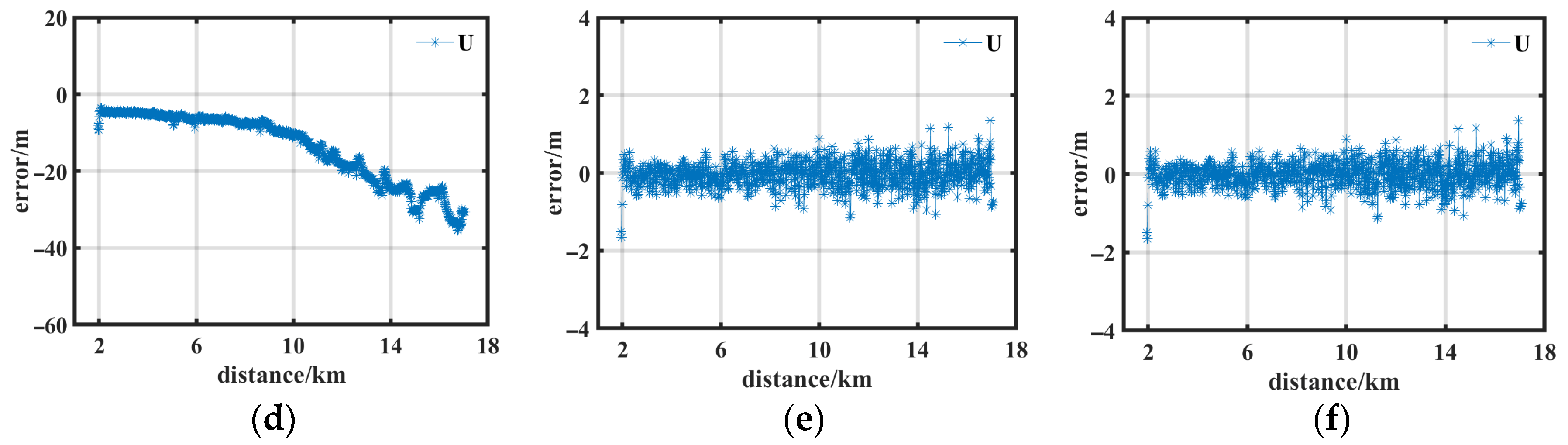
4.1. Experiment at a Water Depth of 300 m

To systematically evaluate the directional accuracy characteristics of three navigation schemes, we established a local east–north–up (ENU) coordinate system. The underwater vehicle executed a diagonal traversal path across the seafloor transponder array at a constant depth of 300 m, performing acoustic ranging at 20 s intervals. Over an 8 h experimental duration, the system acquired four discrete acoustic travel time datasets, each containing 1039 epochs, corresponding to a total horizontal trajectory length of approximately 15 km. Figure 5a comparatively presents the reference trajectory obtained from ultrashort baseline (USBL) positioning against the solutions generated by the three proposed schemes.

As illustrated in Figure 5b, the experiment captured four distinct sets of acoustic ray incidence angles between the transducer and seafloor transponders. Quantitative analysis reveals that the minimum angle of incidence is 7.33°, observed at 1.95 km horizontal offset from the transponder array centroid, and the maximum angle of incidence is 81.32°, recorded at 17.07 km horizontal offset. The angular measurements exhibit a direct proportionality between horizontal distance from the transponder array centroid and the measured incident angles.

The professional navigation standard is an average PDOP of <3.8. As illustrated in Figure 6, during the 420th calendar element, the PDOP remained in the desirable range of 2.0–3.8, corresponding to the vehicle operating within the center of the transponder array. This phase exhibits optimal geometric symmetry and >95% baseline utilization efficiency. After the 420th calendar element, the PDOP increases nearly linearly, with a peak of 14.2. This anomaly arises from the asymmetric distribution of the underwater vehicle as it moves away from the center of the undersea transponder array, resulting in an increase in the PDOP and a corresponding decrease in navigation accuracy.

As illustrated in Figure 7, the navigation errors of the three schemes exhibit consistent trends in the east and north directions, progressively increasing with the distance between the transducer and the four seafloor transponders. A comparative analysis reveals that Scheme 2 and Scheme 3 reduce the droop error from 20.91 m in scenario 1 by 98.41% to 0.33 m with the depth constraint method, and the suppression effects of the two schemes are identical. This phenomenon confirms that the depth constraint can effectively eliminate the vertical error accumulation problem in the traditional model. The strong suppression of vertical error indirectly improves the horizontal positioning accuracy. Scheme 3 further dynamically adjusts the observation weights through the adaptive stochastic model optimization based on SVD, which improves the error suppression effect in the east and north directions by 20.48% and 37.14%, respectively, compared with Scheme 2, reflecting the advantage of the adaptive algorithm in the co-optimization of the complex sea state.

To assess the impact of underwater vehicle–baselines positional relationships on navigation accuracy, we count the navigation accuracy of the underwater vehicle outside the baselines and the navigation accuracy of the underwater vehicle within the baselines, as depicted in

Table 1. The accuracy statistics (RMS) of three schemes at a depth of 300 m.

Underwater Vehicle’s Position	Scheme	RMS-E/m	RMS-N/m	RMS-U/m	RMS-3D/m
Inside Baselines	Scheme 1	1.95	0.36	1.99	2.81
	Scheme 2	1.12	1.02	0.12	1.52
	Scheme 3	0.85	0.52	0.12	1.00
Outside Baselines	Scheme 1	13.76	7.15	20.82	25.96
	Scheme 2	10.05	5.46	0.31	11.44
	Scheme 3	7.99	3.29	0.31	8.65

.

Inside the baselines, the 3D navigation error of Scheme 1 is 2.81 m, with the vertical error accounting for 74.3% of the total error. This demonstrates the fundamental limitations of the traditional method, where vertical errors dominate in underwater acoustic positioning systems. Scheme 2 incorporates vertical depth-constraint mechanisms, effectively suppressing elevation errors to sub-meter levels. This results in a 45.91% overall accuracy enhancement (1.52 m) compared to Scheme 1, demonstrating that prior depth information can eliminate over 78% of traditional model error sources through geometric constraint optimization. Scheme 3 achieves 34.21% further improvement in horizontal positioning accuracy (1.00 m).

Outside the baselines, Scheme 2 and Scheme 3 reduce the vertical error from 20.82 m to 0.31 m (98.51% reduction) by means of depth constraints, which completely solves the vertical dispersion problem of the traditional model. Scheme 3 introduces SVD adaptive weight allocation on the basis of the static constraints of Scheme 2, which reduces the east and north direction errors by another 20.5% and 39.74% compared with Scheme 2, reflecting the ability of the dynamic model to compensate for the geometric weakening outside the baseline. Scheme 3 achieves only 34.21% improvement inside the baseline array, while the accuracy jumps significantly outside the baseline array, which indicates that its adaptive optimization mechanism is more effective under poor geometric conditions.

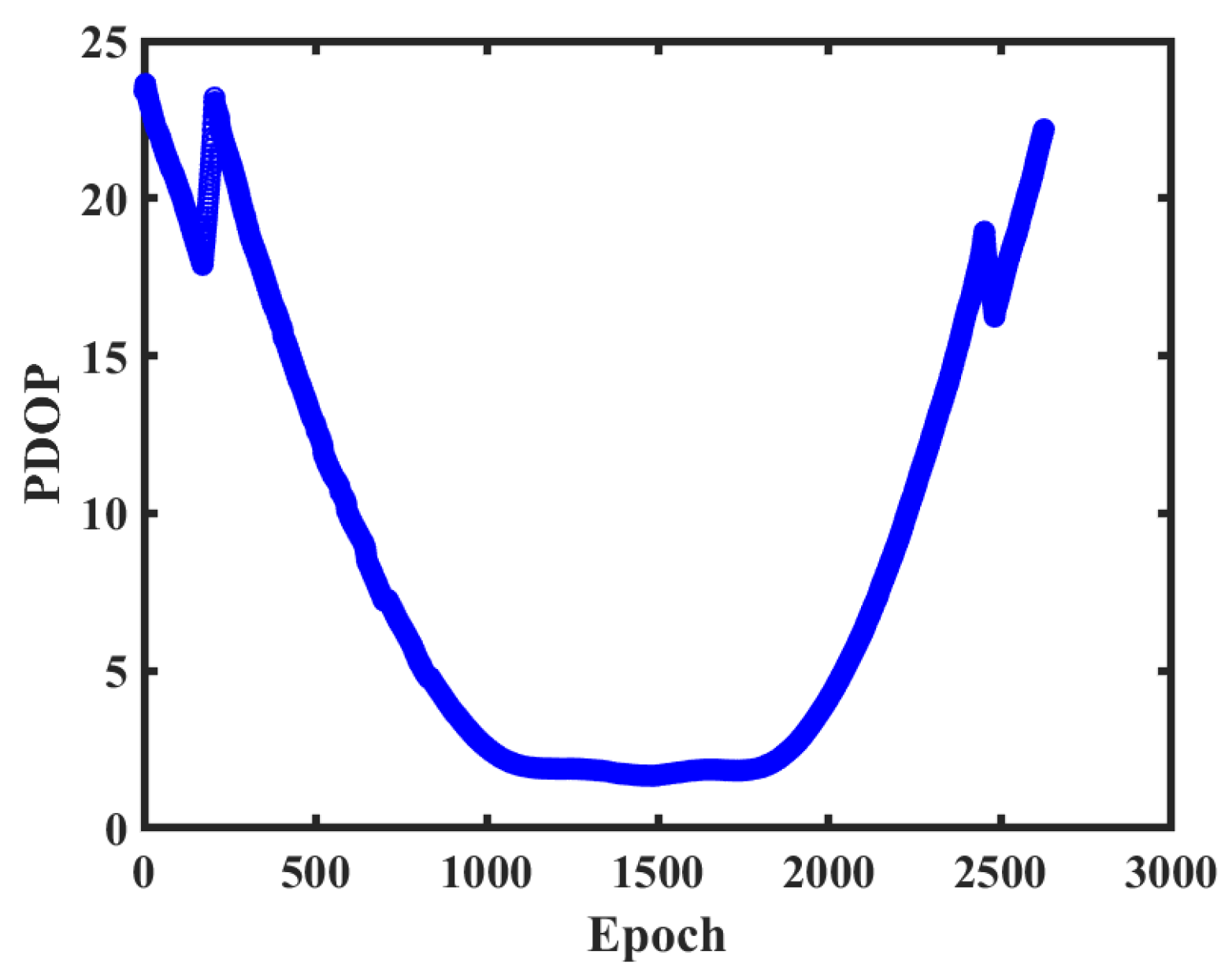
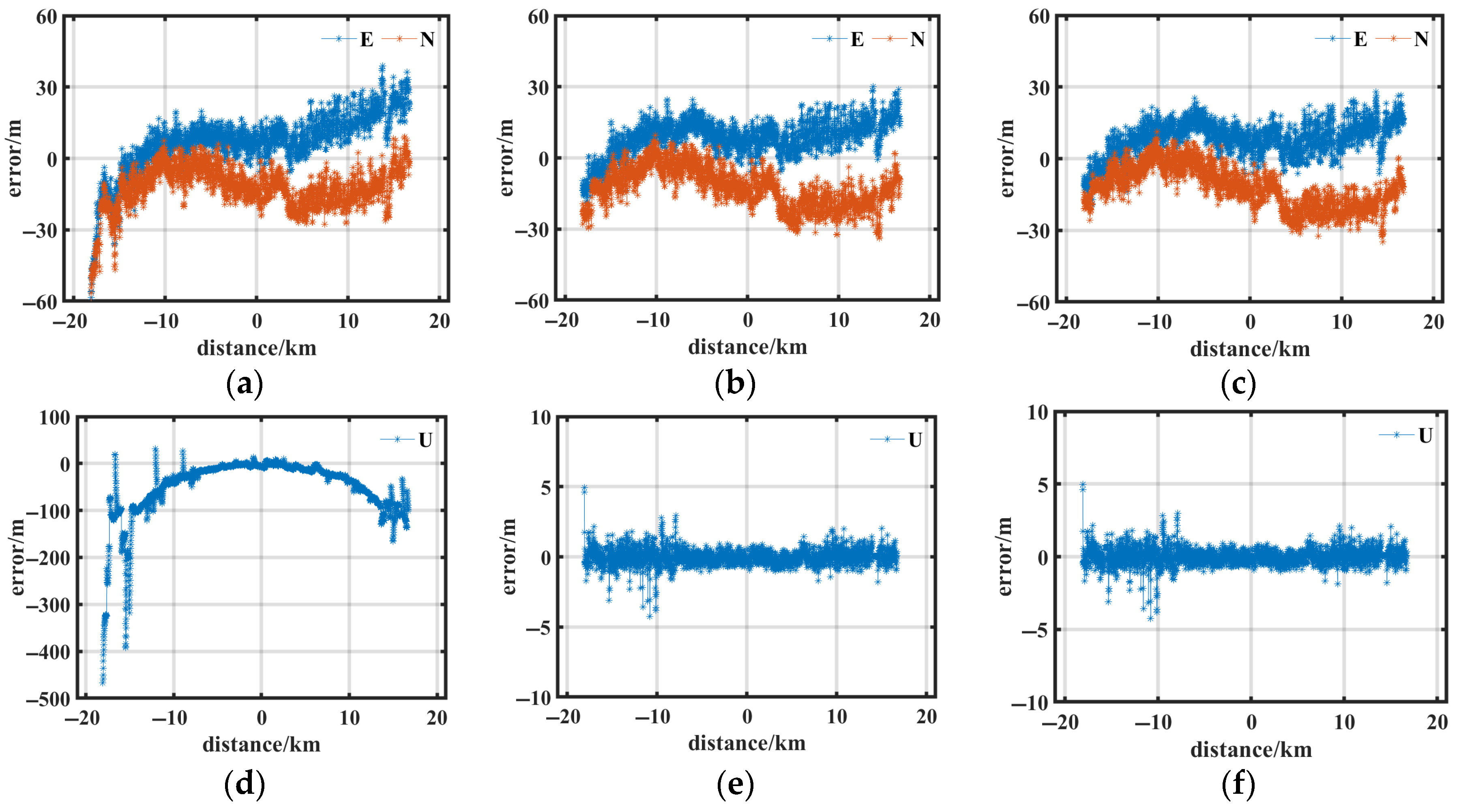
4.2. Experiment at a Water Depth of 2000 m

The underwater vehicle ran along the long diagonal of the seafloor transponders at a water depth of 2000 m, ranging every 20 s. The experiment was conducted for a total time of approximately 15 h and included four sets of acoustic travel time data, of which each set of data had 10,508 epochs. The horizontal length of the trajectory was about 35 km. The navigation trajectory measured by USBL and the trajectory solved by the three schemes are shown in Figure 8a.

Figure 8b reveals four distinct acoustic ray incidence angles between the transducer and seafloor transponders. The minimum incidence angle is 8.46° and occurs at a 0.11 km horizontal distance from the transponder array center, while the maximum angle is 80.36° and is observed at 18.07 km. This angular progression demonstrates a near-linear relationship with horizontal range. Notably, the 8.46° minimum angle approaches the system’s critical threshold for multipath interference mitigation, validating the array’s design for deep-water operations.

Figure 9 reveals the PDOP values, which range from 0 to 25, indicating significantly elevated levels. Notably, 78.3% of the values fall within the high-risk interval of 10–20, suggesting that the transducer is likely positioned near the edge of the transponder array, creating asymmetric observation geometry. Sharp PDOP spikes observed during epochs 170–200 and 2450–2480 correlate with the vehicle’s vertical descent phase. This phenomenon results from rapid deterioration of vertical observability due to dynamic geometric reconfiguration.

As illustrated in Figure 10, Scheme 1 exhibits significant vertical error dominance, with a vertical error of 20.91 m, accounting for 74.3% of its total 26.11 m three-dimensional error. Scheme 2 introduces geometric constraints using depth measurements, reducing vertical error to 0.82 m (98.31% suppression). Scheme 3 further enhances this suppression to 0.33 m by SVD for adaptive noise weighting, achieving a 98.8% error reduction compared to Scheme 1. The vertical error suppression in Scheme 2 and Scheme 3 indirectly improves horizontal positioning through error covariance redistribution. Scheme 3 reduces the errors of the east and north directions by 5.38% and 3.00% compared to Scheme 2, demonstrating the efficacy of its dynamic model adaptation in handling seafloor multipath effects and transducer positioning uncertainties.

To assess the impact of underwater vehicle–baselines positional relationships on navigation accuracy, we count the navigation accuracy of the underwater vehicle outside the baselines and the navigation accuracy of the underwater vehicle within the baselines, as depicted in

Table 2. The accuracy statistics (RMS) of two schemes at a depth of 2000 m.

Underwater Vehicle’s Position	Scheme	RMS-E/m	RMS-N/m	RMS-U/m	RMS-3D/m
Inside Baselines	Scheme 1	4.45	7.14	3.11	8.97
	Scheme 2	4.76	7.47	0.21	8.86
	Scheme 3	4.60	7.39	0.20	8.71
Outside Baselines	Scheme 1	14.28	14.36	80.40	82.91
	Scheme 2	11.13	13.61	1.34	17.63
	Scheme 3	10.49	13.12	1.34	16.85

.

Inside the baselines, the three schemes exhibit less than 2.9% difference in 3D navigation error, attributable to their favorable geometric configuration. This indicates comparable navigation accuracy performance among the schemes under ideal observation conditions.

Outside the baselines, Scheme 2 and Scheme 3 reduce the vertical error from 80.40 m to 1.34 m (98.33% reduction) by means of depth constraints, which completely solves the vertical dispersion problem of the traditional model. Scheme 3 introduces SVD adaptive weight allocation on the basis of the static constraints of Scheme 2, which reduces the east and north direction errors by another 5.75% and 3.60% compared with Scheme 2, reflecting the ability of the dynamic model to compensate for the geometric weakening outside the baseline. Scheme 3 achieves 17 times higher accuracy improvement outside the baselines than inside (east direction: 0.64 m vs. 0.04 m), which critically highlights the necessity of the adaptive algorithm under adverse geometric conditions.

5. Discussion

This study proposes a depth-constrained stochastic model optimization method based on singular value decomposition (SVD), effectively addressing two key limitations in existing underwater acoustic navigation methods:

• Dynamic Covariance Adaptation Mechanism

Traditional extended Kalman filter (EKF) frameworks rely on static noise models, which are prone to error accumulation in complex sound speed fields. Innovatively, this method utilizes SVD to dynamically weight the contribution of each acoustic beacon to the navigation system’s observability space, enabling online adaptive adjustment of the noise covariance. Deep-sea trials demonstrate that this mechanism significantly reduces positioning errors caused by the geometric dilution of precision (GDOP), achieving an error reduction of 40–70%.

2.

Absolute Depth Reference Fusion Mechanism

To address the error divergence in the vertical channel of underwater acoustic navigation systems, this method introduces a centimeter-level accuracy absolute depth reference provided by pressure sensors as a strong constraint. This mechanism fundamentally suppresses vertical error divergence.

Despite the above advancements, the proposed method still faces the following key challenges:

• Time Synchronization Error

The current system assumes that the transducer remains stationary when receiving multiple acoustic signals at different times, neglecting its actual motion. This time synchronization error (or “receiver position error due to motion”) is a major bottleneck for positioning accuracy. Improving timestamp processing for received signals or developing motion compensation algorithms is a key future focus.

2.

Sensor Displacement Induced by Deep-Ocean Currents

Strong ocean currents may displace pressure sensors, causing bias in the provided depth reference (constraint discrepancy). To mitigate this issue, we propose an IMU-pressure sensor coupled with the Kalman filter for a smoother design, aiming to estimate and compensate for displacement by fusing inertial measurement data.

3.

System Integration and Application

Future work will focus on the system-level integration and engineering application validation of the “SVD-EKF Dynamic Optimization Framework” incorporating deep constraint mechanisms, such as embedding the SVD optimization framework into robust Kalman filters, particle filters, or neural network-based modules as inputs into adaptive weighting, or noise modeling to evaluate the localization accuracy, robustness, computational complexity, and real-time performance of these integrated solutions under complex scenarios, such as beacon failures, complex maneuvers, strong non-Gaussian noise, and time-varying multipath effects.

6. Conclusions

In this study, we constructed in detail the acoustic observation matrix between the underwater vehicle and seafloor beacons and proposed an innovative adaptive stochastic model optimization method using SVD. The main conclusions are as follows:

• By establishing a geometric sensitivity analysis framework through SVD of the acoustic observation matrix, we achieved dynamic weighting of the beacon contributions to dominant navigation directions. This approach enables precise suppression of error propagation in both the horizontal and vertical dimensions, particularly addressing the vertical error dominance inherent in conventional equal-weight models.
• The experimental results demonstrate the method’s effectiveness in complex underwater environments. The RMS error reduction (from 2.81 m to 0.93 m) in the 300 m depth scenario is 66.65%, and the RMS error reduction (from 8.04 m to 1.83 m) in the 2000 m depth scenario is 77.25%. These improvements confirm that the proposed method significantly enhances the robustness and navigation accuracy of underwater navigation in complex environments under different underwater acoustic conditions.

Future work will focus on integration of multisource constraints, such as inertial measurements, bathymetric data, etc., within the SVD-EKF architecture, as well as addressing the time synchronization challenge through coupled estimation of motion-induced signal reception delays.

References

1. Yang, Y.; Li, X. Micro-PNT, comprehensive PNT. Acta Geod. Cartogr. Sin. 2017, 46, 1249–1254. [Google Scholar] [CrossRef]
2. Xu, J.; Lin, E.; He, H.; Wu, M. Underwater PNT technology and perspectives. Aerodyn. Missile J. 2021, 6, 139–147. [Google Scholar]
3. Sendra, S.; Lloret, J.; Jimenez, J.M.; Parra, L. Underwater acoustic modems. IEEE Sens. J. 2016, 16, 4063–4071. [Google Scholar] [CrossRef]
4. Yang, Y.; Liu, Y.; Sun, D.; Xu, T.; Xue, S.; Han, Y.; Zeng, A. Seafloor geodetic network establishment and key technologies. Sci. China Earth Sci. 2020, 63, 1188–1198. [Google Scholar] [CrossRef]
5. Liu, J.; Chen, G.; Zhao, J.; Gao, K.; Liu, Y. Development and trends of marine space-time frame network. Geomat. Inf. Sci. Wuhan Univ. 2019, 44, 17–37. [Google Scholar] [CrossRef]
6. Liu, Y.; Li, M.; Liu, Y.; He, X.; Chen, G.; Zhang, L.; Tang, Q. Research progress of seafloor geodetic datum construction technology. Adv. Mar. Sci. 2022, 40, 684–700. [Google Scholar]
7. Busacca, F.; Galluccio, L.; Palazzo, S.; Panebianco, A. A comparative analysis of predictive channel models for real shallow water environments. Comput. Netw. 2024, 250, 110557. [Google Scholar] [CrossRef]
8. Yasuda, K.; Tadokoro, K.; Taniguchi, S.; Kimura, H.; Matsuhiro, K. Interplate locking condition derived from seafloor geodetic observation in the shallowest subduction segment at the Central Nankai Trough, Japan. Geophys. Res. Lett. 2017, 44, 3572–3579. [Google Scholar] [CrossRef]
9. Watanabe, S.-I.; Ishikawa, T.; Yokota, Y.; Nakamura, Y. GARPOS: Analysis software for the GNSS-A seafloor positioning with simultaneous estimation of sound speed structure. Front. Earth Sci. 2020, 8, 597532. [Google Scholar] [CrossRef]
10. Sakic, P.; Ballu, V.; Royer, J.Y. A multi-observation least-squares inversion for GNSS-A seafloor positioning. Remote Sens. 2020, 12, 448. [Google Scholar] [CrossRef]
11. Chadwell, C.D.; Sweeney, A.D. Acoustic ray-trace equations for seafloor geodesy. Mar. Geod. 2010, 33, 164–186. [Google Scholar] [CrossRef]
12. Cao, J.; Zheng, C.; Sun, D.; Zhang, D. Travel time processing for LBL positioning system. In Proceedings of the 2016 IEEE/OES China Ocean Acoustics (COA), Harbin, China, 9–11 January 2016; pp. 1–5. [Google Scholar] [CrossRef]
13. Zhang, Y.; Ji, X.; Zhang, D. Short baseline underwater positioning principle and error. Ship Electron. Eng. 2017, 37, 41–45. [Google Scholar] [CrossRef]
14. Jia, C.; Wen, Q.; Zou, Z.; Nie, Z. Underwater real-time heading determination method by using a dual-beacon design of USBL acoustic positioning. IEEE Sens. J. 2025, 25, 10163–10173. [Google Scholar] [CrossRef]
15. Xia, M.; Zhang, T.; Wang, J.; Zhang, L.; Zhu, Y.; Guo, L. The fine calibration of the Ultra-Short baseline system with inaccurate measurement noise covariance matrix. IEEE Trans. Instrum. Meas. 2022, 71, 1–8. [Google Scholar] [CrossRef]
16. Tian, T. Underwater Positioning and Navigation Technology; National Defense Industry Press: Beijing, China, 2007. [Google Scholar]
17. Zhu, Y.; Zhou, L. Hybrid tightly-coupled SINS/LBL for underwater navigation system. IEEE Access 2024, 12, 31279–31286. [Google Scholar] [CrossRef]
18. Liu, Y.; Xu, T.; Nie, W.; Wang, J.; Shu, J.; Zhang, S.; Yang, W. High-precision LBL/INS round-trip tightly coupled navigation based on constrained acoustic ray-tracking and RTS smoothing. IEEE Trans. Veh. Technol. 2024, 73, 16432–16444. [Google Scholar] [CrossRef]
19. Sato, M.; Fujita, M.; Matsumoto, Y.; Saito, H.; Ishikawa, T.; Asakura, T. Improvement of GPS/acoustic seafloor positioning precision through controlling the ship’s track line. J. Geod. 2013, 87, 825–842. [Google Scholar] [CrossRef]
20. Chen, G.; Liu, Y.; Liu, Y.; Tian, Z.; Li, M. Adjustment of transceiver lever arm offset and sound speed bias for GNSS-A positioning. Remote Sens. 2019, 11, 1606. [Google Scholar] [CrossRef]
21. Yang, Y.; Ming, F. Current status and future development of spatiotemporal datum construction in China. Sci. China Earth Sci. 2023, 66, 2162–2165. [Google Scholar] [CrossRef]
22. Ikuta, R.; Tadokoro, K.; Ando, M.; Okuda, T.; Sugimoto, S.; Takatani, K.; Yada, K.; Besana, G.M. A new GPS-acoustic method for measuring ocean floor crustal deformation: Application to the Nankai Trough. J. Geophys. Res.-Solid Earth 2008, 113, B02401. [Google Scholar] [CrossRef]
23. Fujita, M.; Ishikawa, T.; Mochizuki, M.; Sato, M.; Toyama, S.; Katayama, M.; Kawai, K.; Matsumoto, Y.; Yabuki, T.; Asada, A.; et al. GPS/acoustic seafloor geodetic observation: Method of data analysis and its application. Earth Planets Space 2006, 58, 265–275. [Google Scholar] [CrossRef]
24. Li, X.; Li, W.; Yi, X.; Huang, Q.; Wang, Y.; Ye, C. Path-specific Underwater Acoustic Channel Tracking and its Application in Passive Time Reversal Mirror. arXiv 2021, arXiv:2103.00874. [Google Scholar]
25. Shi, J.; Leau, Y.-B.; Li, K.; Chen, H. Optimal Variational Mode Decomposition and Integrated Extreme Learning Machine for Network Traffic Prediction. IEEE Access 2021, 9, 51818–51831. [Google Scholar] [CrossRef]
26. Sakic, P.; Ballu, V.; Crawford, W.C.; Wöppelmann, G. Acoustic ray tracing comparisons in the context of geodetic precise off-shore positioning experiments. Mar. Geod. 2018, 41, 315–330. [Google Scholar] [CrossRef]
27. Zhao, J.; Zhang, H.; Wu, M. A sound ray tracking algorithm based on template interpolation of constant gradient sound velocity. Geomat. Inf. Sci. Wuhan Univ. 2021, 46, 71–78. [Google Scholar] [CrossRef]
28. Xin, M.; Yang, F.; Xue, S.; Wang, Z.; Han, Y. A constant gradient sound ray tracing underwater positioning algorithm considering incident beam angle. Acta Geod. Cartogr. Sin. 2020, 49, 1535–1542. [Google Scholar] [CrossRef]
29. Zhao, S.; Wang, Z.; Liu, H. Investigation on underwater positioning stochastic model based on sound ray incidence angle. Acta Geod. Cartogr. Sin. 2018, 47, 1280–1289. [Google Scholar] [CrossRef]
30. Yan, F.; Wang, Z.; Zhao, S.; Nie, Z.; Sun, Z.; Li, W. A layered constant gradient acoustic ray tracing underwater positioning algorithm considering round-trip acoustic path. Acta Geod. Cartogr. Sin. 2022, 51, 31–40. [Google Scholar] [CrossRef]
31. Chen, H. Travel-time approximation of acoustic ranging in GPS/Acoustic seafloor geodesy. Ocean Eng. 2014, 84, 133–144. [Google Scholar] [CrossRef]
32. Chen, H.-H.; Wang, C.-C.; Chuang, W.-N.; Lin, B.-H.; Li, K.-H.; Su, J.-D. Linear and bilinear approximations of sound speed profiles in GPS/Acoustic seafloor geodesy. In Proceedings of the IEEE International Underwater Technology Symposium, Tokyo, Japan, 5–8 March 2013; pp. 1–8. [Google Scholar] [CrossRef]
33. Wang, J.; Xu, T.; Nie, W.; Yu, X. The construction of sound speed field based on back propagation neural network in the global ocean. Mar. Geod. 2020, 43, 621–642. [Google Scholar] [CrossRef]
34. Zhao, J.; Zhou, F.; Zhang, H.; Wang, S. Establishment of spatial model for sound velocity in local. Geomat. Inf. Sci. Wuhan Univ. 2008, 33, 199–202. [Google Scholar]
35. Liu, Y.; Wang, Z.; Zhao, S. Layered-EOFs based adaptive reconstruction of sound velocity profile in multi-beam sounding. Tech. Acoust. 2019, 39, 372–378. [Google Scholar]
36. Yang, Y.; Qin, X. Resilient observation models for seafloor geodetic positioning. J. Geod. 2021, 95, 79. [Google Scholar] [CrossRef]
37. Zhao, J.; Zou, Y.; Wu, Y.; Fang, S. Determination of underwater control point coordinates based on the constraint of water depth. J. Harbin Inst. Technol. 2016, 48, 137. [Google Scholar] [CrossRef]
38. Qin, X.; Yang, Y.; Sun, B. A robust method to estimate the coordinates of seafloor stations by direct-path ranging. Mar. Geod. 2023, 46, 83–98. [Google Scholar] [CrossRef]
39. Yang, F.; Lu, X.; Li, J.; Han, L.; Zheng, Z. Precise positioning of underwater static objects without sound speed profile. Mar. Geod. 2011, 34, 138–151. [Google Scholar] [CrossRef]
40. Yang, Y. Resilient PNT concept frame. Acta Geod. Cartogr. Sin. 2018, 47, 893–898. [Google Scholar] [CrossRef]
41. Liu, Y.; Xue, S.; Lu, X.; Wang, X.; Qi, K.; Wang, S. Optimization on underwater positioning stochastic model based on sound ray elevation angle. Hydrogr. Surv. Charting 2021, 41, 21–25. [Google Scholar] [CrossRef]
42. Wang, X.; Xue, S.; Qu, G.; Liu, Y.; Yang, W. Disturbance analysis of underwater positioning acoustic ray and design of piecewise exponential weight function. Acta Geod. Cartogr. Sin. 2021, 50, 982–989. [Google Scholar]
43. Wang, W.; Ouyang, Y.; Ma, Y.; Dong, C. Application of Helmert variance component estimation in underwater acoustic positioning. J. Ocean Technol. 2020, 39, 83–88. [Google Scholar]
44. Meng, Q.; Wang, Z.; Liu, Y.; Wang, B. Application of robust Helmert variance component estimation in underwater acoustic positioning. Hydrogr. Surv. Charting 2019, 39, 70–74. [Google Scholar] [CrossRef]
45. Li, J. Research on Underwater Acoustic Navigation Filtering Algorithm Under Combined State. Master’s Thesis, School of Geological Engineering and Geomatics, Chang’an University, Xi’an, China, 2023. [Google Scholar]
Figure 1. Deployment of the experiment and instruments used in the experiment.
Jmse 13 01329 g001
Figure 2. Horizontal trajectories of the underwater vehicle with depth color information. (a) The depth of 300 m. (b) The depth of 2000 m.
Jmse 13 01329 g002
Figure 3. Two sound velocity profiles.
Jmse 13 01329 g003
Figure 4. Travel time for acoustic signal. (a) The depth of 300 m. (b) The depth of 2000 m.
Jmse 13 01329 g004
Figure 5. (a) The diagram of the trajectory measured by USBL and the trajectory solved by three schemes at a water depth of 300 m. (b) Acoustic ray incident angles between the transducer and the four seafloor transponders.
Jmse 13 01329 g005
Figure 6. Variation in position dilution of precision in an experimental environment at 300 m water depth.
Jmse 13 01329 g006
Figure 7. The navigation error distribution of three schemes at a depth of 300 m. (a) Errors in the east and north directions for Scheme 1, (b) errors in the east and north directions for Scheme 2, (c) errors in the east and north directions for Scheme 3, (d) errors in the up direction for Scheme 1, (e) errors in the up direction for Scheme 2, (f) errors in the up direction for Scheme 3.
Jmse 13 01329 g007aJmse 13 01329 g007b
Figure 8. (a) The diagram of the trajectory measured by USBL and the trajectory solved by three schemes at a water depth of 2000 m. (b) Acoustic ray incident angles between the transducer and the four seafloor transponders.
Jmse 13 01329 g008
Figure 9. Variation in position dilution of precision in an experimental environment at 2000 m water depth.
Jmse 13 01329 g009
Figure 10. The navigation accuracy distribution of two schemes at a depth of 2000 m. (a) Errors in the east and north directions for Scheme 1, (b) errors in the east and north directions for Scheme 2, (c) errors in the east and north directions for Scheme 3, (d) errors in the up direction for Scheme 1, (e) errors in the up direction for Scheme 2, (f) errors in the up direction for Scheme 3.
Jmse 13 01329 g010