Application of Machine Learning for Fuel Consumption and Emission Prediction in a Marine Diesel Engine Using Diesel and Waste Cooking Oil

Abstract

This study creates and tests a machine learning model that can predict fuel use and emissions (NO_x, CO₂, CO, HC, PN) from a marine internal combustion engine when it is running normally. The model learned from data collected from conventional diesel fuel experiments. Subsequently, we evaluated its ability to transfer by employing the parameters associated with waste cooking oil (WCO) biodiesel and its 60/40 diesel mixture. The machine learning model demonstrated exceptional proficiency in forecasting diesel mode (R² > 0.95), effectively encapsulating both long-term trends and short-term fluctuations in fuel consumption and emissions across various load regimes. Upon the incorporation of WCO data, the model maintained its capacity to identify trends; however, it persistently overestimated emissions of CO, HC, and PN. This discrepancy arose primarily from the differing chemical composition of the fuel, particularly in terms of oxygen content and density. A significant correlation existed between indicators of incomplete combustion and the utilization of fuel. Nonetheless, NO_x exhibited an inverse relationship with indicators of combustion efficiency. The findings indicate that the model possesses the capability to estimate emissions in real time, requiring only a modest amount of additional training to operate effectively with alternative fuels. This approach significantly diminishes the necessity for prolonged experimental endeavors, rendering it an invaluable asset for the formulation of fuel strategies and initiatives aimed at mitigating carbon emissions in maritime operations.

1. Introduction

Machine learning (ML) is becoming a must-have technique in the marine industry for modeling, predicting, and improving the performance and emissions of internal combustion engines (ICEs) [1]. As the need to cut down on greenhouse gases and meet the strict emission standards set by the International Maritime Organization (IMO) grows, neural networks are becoming more important as real-time, very accurate ways to manage emissions [2,3]. Recent studies have shown that machine learning (ML), especially when used with other advanced algorithmic frameworks, can forecast NO_x, CO, HC, and PN emissions as well as fuel consumption with very high accuracy under a wide range of load situations [4].

The DASVR method is one of the most advanced because it combines the capacity of ML to find nonlinear relationships with the speed of SVR in low-dimensional spaces. In a study using the DASVR algorithm, models were developed to predict BSFC as well as NO_x, PN, HC, and CO emissions. They were characterized by a maximum error level not exceeding 3.8%, and real-time factors remained R² < 0.96 even at engine speeds <3000 rpm. DASVR was not only more accurate than traditional ML and SVR approaches, but it also worked faster [5,6]. Also, ML models used in earlier studies for internal combustion engines (ICEs) showed amazing outcomes. In a study that used a mini-diesel engine test system with a hydraulic dynamometer, the ML model obtained regression coefficients of R² > 0.9 for both SFC and BTE forecasts. For emissions predictions (CO₂, NO_x), the R² values went up to 0.99933. The biggest differences were less than 7% for SFC and less than 6% for BTE [7].

The same study found that a simple ML architecture with 10 neurons in the hidden layer avoided overfitting, generalized the data well, and showed the best engine operating points. The model predicted that BTE could be increased by up to 49.92% and SFC reduced by up to 0.27 kg/kWh. This resulted in up to 12% higher thermal efficiency and 40% lower CO emissions. In addition to the technical benefits, this approach significantly reduces the number of tests in the laboratory, reducing costs and increasing safety [2,7].

Equally important is the application of ML in complex engine dynamics [8]. In studies using ML in conjunction with control algorithms such as MPC (Model Predictive Control), neural networks have been integrated into emission control architectures. For example, an ML model predicting NO_x and soot emissions was integrated with the GT-Power airpath model. It built a low-order LPV model that lets you change the EGR and manifold pressure targets to obtain the best emissions without having to buy expensive sensors [9].

Another example is using ML models to figure out how much pollution bioethanol-enriched fuels cause. ML models found the best circumstances for a 16.7% drop in NO_x emissions and a big drop in soot content by mixing varying amounts of bioethanol and EGR. ML also assisted in modeling the complicated relationship between the amount of oxygen available and the type of fuel used [10].

When used in Digital Twin architecture, ML also shows how flexible it is. Researchers used ML models and optimization algorithms like NSGA III in a study that looked at how to forecast aging processes like injector wear. We were able to obtain a 4% inaccuracy in predicting actuator displacements and less than 0.9% in response deviations. [11].

In general, the application of ML allows for the prediction of both physical and chemical engine parameters based on a limited number of sensors [12,13,14]. In one study, ML models were trained with only five sensors and were able to predict as many as 16 different engine and emission parameters. This is particularly important for unmanned DGs (diesel generators), where sensor replacement is not possible. The results of this work show that ML-based models are not only accurate (R² > 0.92), but also stable under different operating conditions [15].

Combining ML with advanced optimization methods like MORSM, genetic algorithms (GAs), and XGBoost lets you look at systems in more depth. Using machine learning to forecast emissions from alternative fuels is an important area of research. Using machine learning architecture was estimated the efficiency of a B25 (25% biodiesel) fuel blend. The average R² factor for emissions was 0.967, and emissions (CO, NO_x, HC) were lowered without a big drop in efficiency [16].

ML-based prediction of HVO and WTPO biofuels allowed the prediction of not only emissions, but also performance changes, depending on the mixture ratio, viscosity, or cetane number. It has been found that ML can be adapted even for small displacement engines if the model is supplemented with the influence of fuel parameters [17,18].

ML models are also integrated with CCUS prediction algorithms. Studies suggest using ML to optimize CO₂ recovery based on real-time route, wind, and fuel consumption data, allowing CCUS systems to operate more efficiently [19]. This allows ML algorithms to be used as the core of real-time CCUS operation optimization.

Furthermore, ML is being implemented in ship digital twins that cover the entire operational profile (speed, load, weather conditions, fuel type). This has enabled the development of real-time emissions prediction systems that help plan more efficient routes and optimize engine performance [20,21].

The novelty of this study is the assessment of machine learning model transferability between conventional diesel fuel and biodiesel made from waste cooking oil (WCO). Unlike most previous studies, which train models independently for each fuel type, we investigate whether a model trained purely on diesel data can accurately forecast emissions from WCO fuel. This method enables us to measure emission sensitivity to fuel composition and identify which emission indicators are most affected, yielding new insights into practical applications such as pollution control, digital twins, and maritime fuel strategy development.

2. Materials and Methods

2.1. Machine Learning Approach

Linear regression model (LRM) as a machine learning (ML) approach was chosen. The main ML aim is to learn from experience $E$ with respect to a task $T$ and performance measure $P$, such that its performance on $T$, as measured by $P$, improves with more experience $E$ [22]. In this study case, for LRM, the task $\left(T\right)$ is to predict a continuous target variable y (e.g., emission levels) based on input $X$; LRM learns from a dataset consisting of input–output pairs $(X,y)$ and it can be called experience $\left(E\right)$. In general, a trained LRM can use unseen data by applying the learned parameters to predict emission outcomes. The LRM development methodology is clearly defined in the methodology section. For each emission type, i.e., NO_X, CO₂, CO, HC, PN, and fuel consumption, LRMs were developed. Load (%) and rotational speed (rpm) were chosen as independent prognostic factors. Experiment data was split into two datasets: training and test. Data gathered from experiments with pure diesel was used only for model training, while data gathered from experiments with fuel mixture was used for model testing. Model testing was performed using unseen data. Regression models were based on the analysis of variance (ANOVA) model [23,24]. The initial model for training the linear regression model and estimating prognostic parameters was defined as follows:

$$Y_i=a+b·L+c·R+\epsilon ,$$

(1)

where $Y_i$—value of engine emission, $i$—type of engine emission parameter, $L$—engine load (%), $R$—rotational speed (rpm), $a$—regression intercept value, $b$—regression parameter for engine load, $c$—regression parameter for rotational speed, $\epsilon$—random error.

The regression parameters estimated during model training were used for model testing. After parameter estimation, a new prognostic model for test set was built [25,26]:

$$Y_i^m=a+b·L^m+c·R^m+{\epsilon }^m,$$

(2)

where $Y_i^m$—value of engine emission, $i$—type of engine emission parameter, $m$—training model for mixture fuel, $L^m$—engine load (%), $R^m$—rotational speed (rpm), $a$—regression intercept value, $b$—regression parameter for engine load, $c$—regression parameter for rotational speed, ${\epsilon }^m$—calculated random error.

Calculated random error was added to the test model in order to maintainbasic ANOVA assumption. The error was generated using the variances calculated for the respective emissions:

$${\sigma }^2={\displaystyle \frac{1}{N}}\sum _{j=1}^N{(y_j-\overline{y})}^2{R}^m+{\epsilon }^m,$$

(3)

where $N$—sample size, $y_j$—observed value of emission parameter $j$, $\overline{y}$—mean of emission parameter.

Next, the random errors distributed according to Gaussian distribution ($N(\mu ,{\sigma }^2)$) were calculated and added to prognostic model [27]:

$$f(x|\mu ,{\sigma }^2)={\displaystyle \frac{1}{\sigma \sqrt{2\pi }}}{e}^{-{\displaystyle \frac{1}{2}}{\left({\displaystyle \frac{x-\mu }{\sigma }}\right)}^2},$$

(4)

where ${\sigma }^2$—variance of emission parameter $j$, $\mu$—mean of emission parameter.

In this study, four prediction accuracy and model fit metrics were used:

• Root mean square error (RMSE);
• Mean absolute error (MAE);
• Mean absolute percentage error (MAPE);
• Coefficient of determination ($R^2$).

The root mean square error (RMSE) quantifies the difference between a model’s predicted values and the actual observed values:

$$RMSE=\sqrt{{\displaystyle \frac{\sum _{j=1}^N{(y_j-\widehat{y_j})}^2}{N}}},$$

(5)

where $N$—sample size, $y_j$—observed value of emission parameter $j$, $\widehat{y_j}$—predicted value of emission parameter $j$.

The mean absolute error (MAE) measures the difference between actual and predicted values, calculated as the average of the absolute differences across the dataset:

$$MAE={\displaystyle \frac{\sum _{j=1}^N|y_j-\widehat{y_j}|}{N}},$$

(6)

where $N$—sample size, $y_j$—observed value of emission parameter $j$, $\widehat{y_j}$—predicted value of emission parameter $j$.

The mean absolute percentage error (MAPE) is a relative error metric that employs absolute values to prevent positive and negative errors from offsetting each other and uses relative errors to facilitate comparison of forecasting accuracy across different time-series models:

$$MAPE={\displaystyle \frac{1}{N}}\sum _{j=1}^N\left|{\displaystyle \frac{y_j-\widehat{y_j}}{y_j}}\right|,$$

(7)

where $N$—sample size, $y_j$—observed value of emission parameter $j$, $\widehat{y_j}$—predicted value of emission parameter $j$.

The coefficient of determination, denoted as $R^2$, is a statistical metric in regression analysis that quantifies the proportion of variance in the dependent variable that is explained by the independent variable(s):

$$R^2=1-{\displaystyle \frac{{SS}_{res}}{{SS}_{tot}}},$$

(8)

$${SS}_{res}=\sum _{j=1}^N{(y_j-\widehat{y_j})}^2,$$

(9)

$${SS}_{tot}=\sum _{j=1}^N{(y_j-\overline{y})}^2,$$

(10)

where $N$—sample size, $y_j$—observed value of emission parameter $j$, $\widehat{y_j}$—predicted value of emission parameter $j$, $\overline{y}$—mean of emission parameter.

Statistical analysis was performed using the Statistical Analysis System (SAS Institute, Cary, NC, USA) package, version 9.2 and RStudio package (version 2023.09.1+494).

2.2. Experiment Methodology

The object of the study was a mixed passenger–cargo ferry built in 2009 in the Republic of Bulgaria, in the city of Burgas [28]. The ship is 52.00 m long, 14.00 m wide, with a maximum draft of 3.40 m. It is capable of transporting up to 400 passengers and 33 vehicles. The structural material—welded steel—ensures structural rigidity, but also determines a significant mass, which in turn increases the load on the engines. The ferry runs on an inland waterway route where the speed and engine load change often, which makes it perfect for dynamic emission investigations.

The ship’s propulsion system consists of two VOLVO PENTA D16-MH (Volvo Group, Skövde, Sweden) main power plants with a total rated power of 2 × 478 kW. These are four-stroke, direct injection, six-cylinder diesel engines with a turbocharger and an intercooler. They are directly connected to two HRP 4000 azimuth thrusters (ADS van STIGT, Gorinchem, The Netherlands), which allow for an effective change in sailing direction and make it possible to avoid an additional steering system.

Additional power supply is provided by two SISU 420 DSRGM auxiliary engines (AGCO SISU POWER, Linnavuori, Finland) (2 × 75 kW), operating as electric generators. They serve the electrical needs of internal systems, lighting, and navigation equipment, and function as an additional source of emissions, especially when were used. Emission and fuel consumption data were collected during both steady cruising (at ~15 km/h) and maneuvering phases (0–20 km/h) in one direction over a typical test route 2.6–2.8 km long, with successive repetition of several tests, allowing for the assessment of emissions changes in different modes. During the study, real-time measurements were performed while the vessel was moving at a constant speed (~15 km/h) and in maneuvering mode (speed changed from 0 to 20 km/h).

This vessel was operated on an inland waterway route characterized by periodically changing loads, frequent maneuvering modes, and short crossing intervals. Such an operating environment is particularly suitable for studies on the dynamics of emissions and engine parameters, as it allows the analysis of the behavior of marine internal combustion engines operating under real conditions in various load situations. The test bench is provided in Figure 1.

The emission parameters were measured in real time using a combination of the Testo 350-MARITIME exhaust gas analyzer (Entech Industrial Solution Co., Ltd., Bangkok, Thailand) and a separate optical particle counter. Nitrogen oxides (NO_x) were measured using an electrochemical sensor with an accuracy of ±0.5 ppm. Carbon dioxide (CO₂) concentrations were determined using a non-dispersive infrared (NDIR) sensor, which provided a measurement accuracy of ±0.2% of the reading. Carbon monoxide (CO) was also measured by an electrochemical sensor, with an accuracy of ±10 ppm or ±5% of the measured value, depending on concentration range.

Hydrocarbons (HCs) were detected using the integrated sensor module within the Testo 350-MARITIME system, offering an accuracy of ±10 ppm or ±5%, depending on the calibration settings and VOC concentration. The particle number (PN) in the exhaust gas was measured using an optical diffusion-based particle counter. This sensor provided a resolution of approximately 1 × 10³ particles per cubic centimeter (particles/cm³), with an estimated accuracy of ±10%, depending on sampling flow rate and calibration conditions. It is important to note that PN measurements represent the total number of particles, without specifying their mass or chemical composition. Fuel consumption was measured by AVL Fuel Mass Flow Meter with ±0.12% accuracy.

Data recording was performed using the data acquisition system “DATAQ DI-718Bx USB DAQ”, connected to variable flow and emission sensors.

During the measurements, the aim was to ensure a stable operational state of the vessel, avoiding external disturbances, such as external winds, strong currents, or nearby vessels. The testing conditions corresponded to typical operating conditions; therefore, the obtained data reasonably reflects the real characteristics of emission generation and allows for reliable application of neural network prediction models.

2.3. Fuel Properties

Two types of fuel with different properties were used in the study: standard petroleum diesel (diesel) and biodiesel obtained from purified used cooking oil (WCO—waste cooking oil). Both fuels have unique physicochemical properties that determine the course of combustion processes, emission intensity, and engine efficiency.

Traditional diesel is widely used in internal combustion engines, complies with the EN590 standard, and is characterized by a high calorific value (~43.2 MJ/kg), a sufficiently high cetane number (~55) and a relatively low density (about 840 kg/m³). These properties ensure stable energy production, rapid ignition, and efficient fuel use [29,30]. Diesel is practically oxygen-free, therefore the amount of emissions during its combustion depends only on external parameters—air content, pressure, and temperature [31]. In addition, due to its extremely low sulfur content (ULSD class), this fuel meets the strict emission standards of the IMO and the European Union.

In the interim, WCO-based biodiesel represents a renewable biofuel synthesized through the amalgamation of methanol or ethanol with various other chemical compounds. This technique converts the fatty acids present in the oil into methyl esters, commonly referred to as FAME. In contrast to diesel, WCO biodiesel exhibits a greater density (approximately 877 kg/m³), a reduced calorific value (37.1 MJ/kg), and an elevated cetane number (around 56) [32,33]. This indicates that this biofuel combusts with greater rapidity and consistency, making it particularly suitable for engines that do not require high speeds [34].

The high oxygen concentration of WCO biodiesel, which falls between 11 and 12%, represents one of its most significant characteristics. This leads to a more efficient combustion process, a decrease in carbon monoxide and hydrocarbon emissions, as well as a reduction in particulate matter [35]. Nonetheless, in alternative scenarios, the combustion temperature is heightened, leading to a rise in NO_x emissions. This biofuel exhibits a sulfur concentration of approximately 0.6%, significantly lower than the sulfur content found in conventional fuels prior to the implementation of ULSD regulations [36,37]. This lowers the danger of SO_x emissions.

The chemical composition shows that WCO biodiesel contains about 81% carbon, 11.7% oxygen, 6.5% hydrogen, and only 0.6% sulfur. This composition indicates that less CO₂ is formed during combustion than from diesel, although, due to the lower energy content per kilogram, this effect can be partially compensated by a higher fuel flow [38,39].

From a practical point of view, WCO biodiesel is particularly suitable for use as an additive to diesel (e.g., a 60/40 mixture). In this case, sufficient thermal efficiency is maintained, but emissions are significantly reduced. In addition, a higher cetane number improves cold start properties, and a higher density ensures higher injector loading, which can positively affect combustion homogenization [38,40].

The diesel fuel employed in this investigation conforms to EN590 standards. The substance exhibits a density approximately measuring 840 kg/m³, alongside a notable lower heating value (LHV) of 43.2 MJ/kg, and a cetane number nearing 55. The WCO biodiesel exhibits a greater density, approximately 877 kg/m³, and a marginally elevated cetane number, around 56. Still, its lower heating value drops a lot to about 37.1 MJ/kg. This is because of the way its molecules are arranged in its composition.

The amount of oxygen is a big difference. Diesel has very little oxygen in fuel, whereas waste cooking oil biodiesel has about 11.7% oxygen by mass. When there is natural oxygen available, the combustion process works better, which means that less carbon monoxide and unburned hydrocarbons are released into the air. But it could also raise the temperature of the combustion process, which could lead to more NO_x being formed.

Ultra-low sulfur diesel fuel (ULSD) has less than 0.001% sulfur in it. WCO biodiesel has about 0.6% sulfur, which is a lot less than regular fuels until ULSD came out. In terms of its elemental makeup, diesel is made up of around 86% carbon and 13% hydrogen by weight. About 81% of WCO biodiesel is carbon, 6.5% is hydrogen, and 11.7% is oxygen.

3. Results

The analyses presented include both an assessment of the accuracy of the ML model in predicting fuel consumption and emission parameters using diesel, as well as an analysis of the transferability of the model when WCO biodiesel parameters were entered into the same model, and the results were compared with experimental data.

3.1. Model Training Results

When analyzing the operating parameters of an internal combustion engine, one of the most important indicators evaluated remains fuel consumption. Figure 2 reflects the dynamics of experimental (blue) and machine learning (ML) model-predicted (red) fuel consumption in the presence of diesel fuel. Figure 2 has more than 1900 measurement points that indicate how the engine works at different speeds and loads.

The findings reveal that the ML model was very good at forecasting how much fuel would really be used. The model could show both big, long-term changes in consumption and smaller, short-term changes. This is very crucial for marine engines, as the way they work changes all the time based on the weather, the way the boat is sailing, the load, or the need to navigate.

Figure 2 shows that fuel use changed between about 165,000 and 285,000 g/h, with most of it happening between 210,000 and 250,000 g/h. The ML model reproduced the data behavior in this central consumption zone particularly accurately. This indicates that the training data contained the largest number of training cases in this area, so the model formed well-defined correlations between the input parameters (speed, load, fuel pressure, etc.) and the response—fuel consumption [41].

Figure 3 shows four clearly segmented operating zones—this allows us to assume that the tests were carried out at different engine load or speed modes, e.g., 100%, 75%, 50%, and 25% of the nominal load. Such testing of load modes is necessary to accurately assess the dynamics of emissions under various operating conditions.

In most sections, the ML model maintains high accuracy, with minimal deviations from the actual values. This indicates that the model is properly trained for all key operating points and is able to adapt to changes in emission intensity.

It is observed that the absolute value of CO₂ emissions decreases when moving from the first zone (about 300–320 g/kWh) to the last (about 100–125 g/kWh). This phenomenon corresponds to the physics of engine operation: as the load decreases, the specific intensity of fuel consumption increases [42,43], but the absolute mass of fuel burned over time decreases, and therefore CO₂ emissions per kilowatt decrease [44]. The ML model successfully reflects this odd but logical relationship between energy efficiency and emissions.

The model remains dependable even when the mode undergoes rapid changes. For instance, while the distinction between the 1–2 and 2–3 operating segments is stark, the model is capable of rapidly adapting to the new circumstances. This implies that the model design has sufficient generalization capabilities to prevent an excessive dependence on individual input data.

Particularly in the transition zone, certain figures may be inaccurate. This could be due to the fact that the engine emissions’ response to a change in load may not be the same, for example, if the combustion temperature or air/fuel ratio changes temporarily. These changes are important in the real world, but an ML model may have trouble predicting them if the sensor data does not show how the microprocesses evolve over time.

The presented Figure 4 reflects the comparison of carbon monoxide (CO) emissions predictions and actual data in different engine operating modes. CO emissions are one of the main pollution indicators of internal combustion engines, and their control is directly related to the efficiency of the combustion process, the air–fuel mixture ratio, and the combustion temperature.

Figure 4 clearly shows four working zones, each of which stands for a particular engine load or combustion mode. As the load lowers or the conditions for combustion improve, the engine runs better, which is why CO emissions go down from about 300 g/kWh to about 100 g/kWh. Typically, at higher loads or suboptimal air–fuel ratios, CO emissions increase due to incomplete fuel combustion. This is noticeable in the first section of the graph, where CO emissions reach their highest values.

A ML model trained using experimental diesel combustion data accurately reproduced the dynamics of CO emissions in all four zones. In each section, it can be seen that the predicted curve (red) closely follows the actual one (blue)—both the average emissions and the local variation [45]. This shows that the ML model is able to identify subtle nuances of the data structure related to the non-idealities of the combustion process.

An important aspect—the closeness and consistency of the data distribution—shows that the ML model has not only learned the average CO emissions level in each operating zone, but is also able to adapt to momentary deviations. However, it can be observed that at the transition points between zones (e.g., between ~5000 and ~5200 experiments), there are short-term dispersion spikes—this is possibly associated with transient operating modes, when the air–fuel balance changes abruptly, and the ML model responds with a slight delay. Nevertheless, the amplitude of the prediction error remains limited, without systematic deviation.

Results of this type are particularly important when it comes to the operational reliability of ML models. Due to their dynamic nature, CO emissions are often more difficult to predict than, say, CO₂ or NO_x, so the high accuracy of this model demonstrates its potential for integration into real-time emission monitoring or control systems [46]. Such a model can be particularly useful in ships where instantaneous transitions between modes are possible (e.g., during port maneuvering), and CO emissions must be actively managed at that time.

The diagram in Figure 5 visualizes the dynamics of hydrocarbon (HC) emission intensity (g/kWh) by comparing the observed values with the values predicted by the ML model in different engine operating modes. HC emissions are directly related to incomplete fuel combustion at low temperatures, improper air–fuel ratio, or short combustion time, therefore their analysis allows assessing the efficiency of the combustion process.

Figure 5 distinguishes four clear operating zones corresponding to different engine load levels or speed modes. In each of the zones, the corresponding HC emission level is recorded, which decreases from ~140 g/kWh in the first section to ~40 g/kWh in the last. This is consistent with the known trend—as engine efficiency increases or combustion conditions improve, HC emissions decrease.

The model’s ability to quickly adapt to regime transitions is also remarkable. As can be seen between 5000 and 5500 as well as 10,000 and 10,500 experimental points, the HC emission level changes abruptly, but the ML model adapts to the new regime without significant delay, without providing distorted or perinertial predictions.

Among the possible sources of model inaccuracy, several individual points or short segments can be distinguished, where the observed HC values suddenly increase or decrease, and the model curve does not fully reflect these fluctuations [47]. Such deviations can be explained by the dynamics of the real process—for example, combustion suppression could have occurred at that time due to an interruption in the fuel supply, excessive EGR flow, or a sudden change in external conditions (humidity, temperature) [48,49]. These phenomena are not directly visible in the sensors, so the ML model cannot predict them.

Nevertheless, the overall performance of the model remains extremely stable—it can be seen that in all four zones, it captures the average of emissions and the natural dispersion without systematic bias [50]. The predictions not only reproduce the emission level with sufficient accuracy, but also correspond to the physical logic of these emissions—lower HC emissions with higher combustion quality and efficiency [51].

The performance of this type of ML model is particularly important for real-time emission monitoring on marine vessels. HC emissions usually arise, not from continuous combustion, but from transient regimes, therefore their prediction is more complicated than for CO₂ or CO. The ability to predict an increase in emissions before it occurs—for example, when approaching the threshold of poor combustion—allows for timely response by changing operating points or combustion strategy [52,53,54].

Nitrogen oxides (NO_x) are one of the most important parts of emissions from internal combustion engines [51,55]. These emissions have a big effect on air pollution and human health. Thus, being able to accurately foresee and control them is an important aspect of the plan to cut down on ship emissions [56,57]. The diagram presented in Figure 6 visualizes the NO_x emission values (g/kWh) by comparing the actual data (blue curve) and the machine learning (ML) model predictions (red curve) under diesel fuel conditions.

Unlike other pollutants, NO_x emissions are characterized by a strong dependence on the combustion temperature and excess air factor. Therefore, they often increase at higher loads, higher engine speeds, or more effective combustion pressures—a trend that is clearly visible in this graph: as the experiment progresses, the NO_x emission level increases from approximately 5000 g/kWh to 8000 g/kWh.

Most importantly, the ML model clearly reproduces this long-term trend in emissions. In both low- and high-emission areas, the model predictions are close to the observed values, which indicates that the model has successfully identified the most important factors determining the formation of NO_x emissions. In all zones (low, medium, and high NO_x intensity), the model provides fairly stable and accurate predictions.

It is worth noting some differences between the curves. Between 7000 and 9000 experiments, momentary fluctuations are observed, when the actual values are slightly more divergent from the general trajectory. This may be related to short-term instabilities in the combustion process, for example, due to changing EGR flow, intake air temperature, or load microtransitions. Such conditions are more difficult to predict if the sensors do not record enough details.

Despite these episodic differences, the model does not show systematic deviation—i.e., the predictions are not consistently higher or lower than the actual values. This indicates that no data overfitting was performed during training and the model retains the ability to generalize beyond the training data.

Figure 7 illustrates the results of the prediction of particulate matter (PN) emissions, comparing the actual (observed) and machine learning (ML) model-predicted (predicted) values, expressed in g/kWh. PN emissions are of great environmental importance, as they have a direct impact on air quality, health, and compliance with IMO requirements, and therefore their accurate assessment is an essential component of any ship emissions analysis.

The data structure shows that at least four clear operating zones were covered during the study. In each of them, the PN emission level decreases steadily—from about 44–45 g/kWh at the beginning to about 25 g/kWh at the end. This trend logically corresponds to decreasing engine load or cleaner combustion conditions. In addition, when the load decreases, more excess air is often introduced, which improves the completeness of combustion and reduces the amount of unburned particles in the exhaust gas.

The ML model predictions in this case are distinguished by high accuracy—both in each individual operating zone and in transient regimes. The red curve (forecast) closely follows the blue (fact), which confirms that the model has successfully processed and learned the essential data relationships. Even in the presence of momentary emission fluctuations—which, in the case of PN, are inevitably due to the non-uniformity of soot combustion—the model response remains stable, without overestimating or over-adjusting short-term anomalies.

It is particularly significant that PN emissions are one of the most difficult emission categories to predict, as they depend on complex microprocesses such as fuel evaporation, mixture homogenization, combustion initiation, and extinction dynamics [58]. Therefore, the ability of the ML model to maintain accuracy in this area indicates that it has properly incorporated significant input variables (e.g., combustion duration, pressure change rate, fuel mass flow).

When assessing the quality of the prediction over the entire testing interval, no systematic deviation is observed—the model maintains average emissions and does not have a clear tendency to constantly exceed or underestimate the actual values. At the transition points (e.g., around the 5000, 10,000, and 15,000 experimental limits) the curves also remain close to each other, which indicates that the model not only generalizes stable operating states, but also recognizes their changes.

This result shows that the ML model is suitable for use in real-time PN emission prediction. This is especially relevant for the control of SCR or DPF systems, where it is necessary to monitor the PN intensity and predict its changes before the emission reduction systems intervene. Such a model can also be integrated into digital twins, allowing the modeling of the operational emission behavior of a ship on different routes or fuel mixtures.

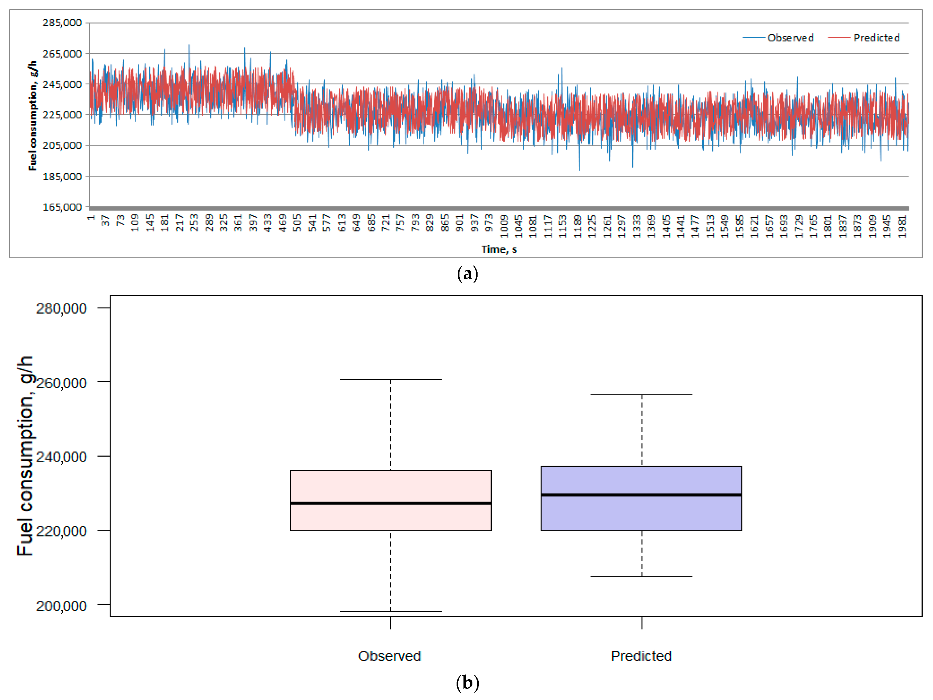
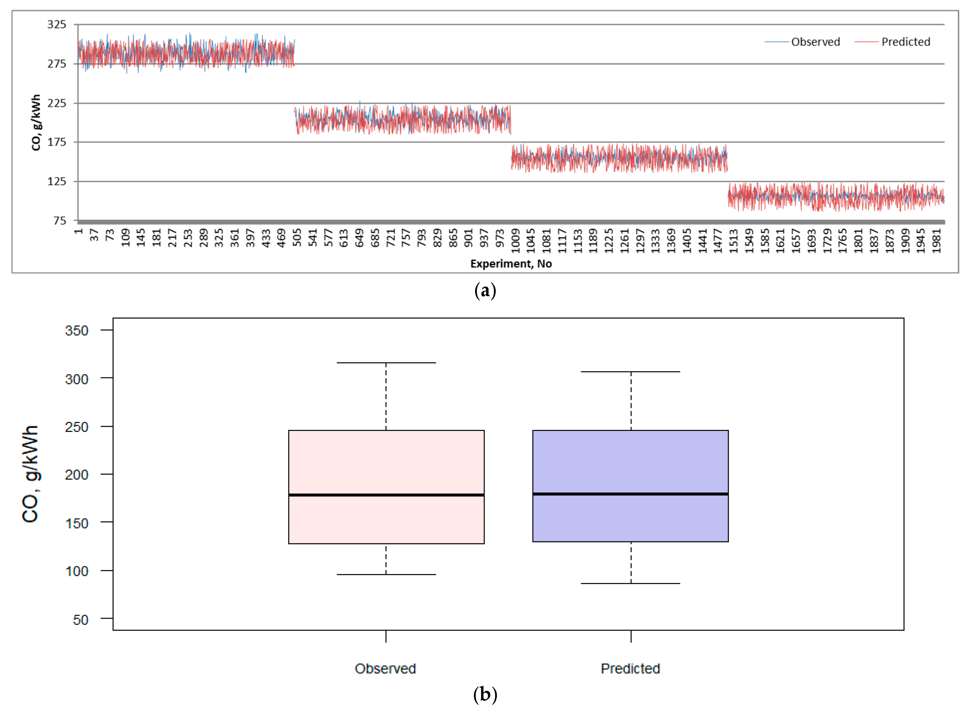
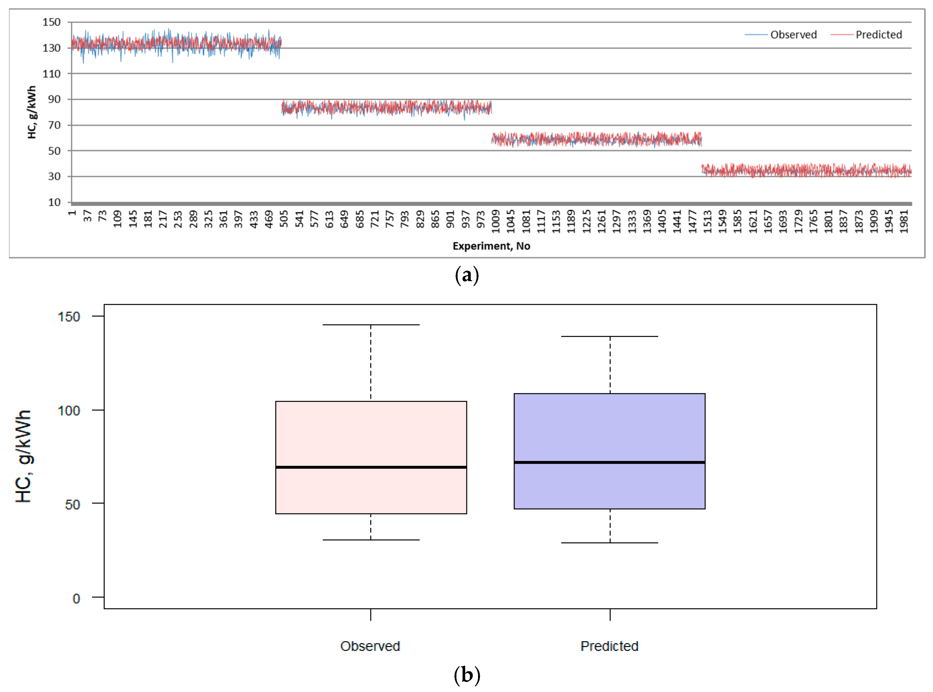
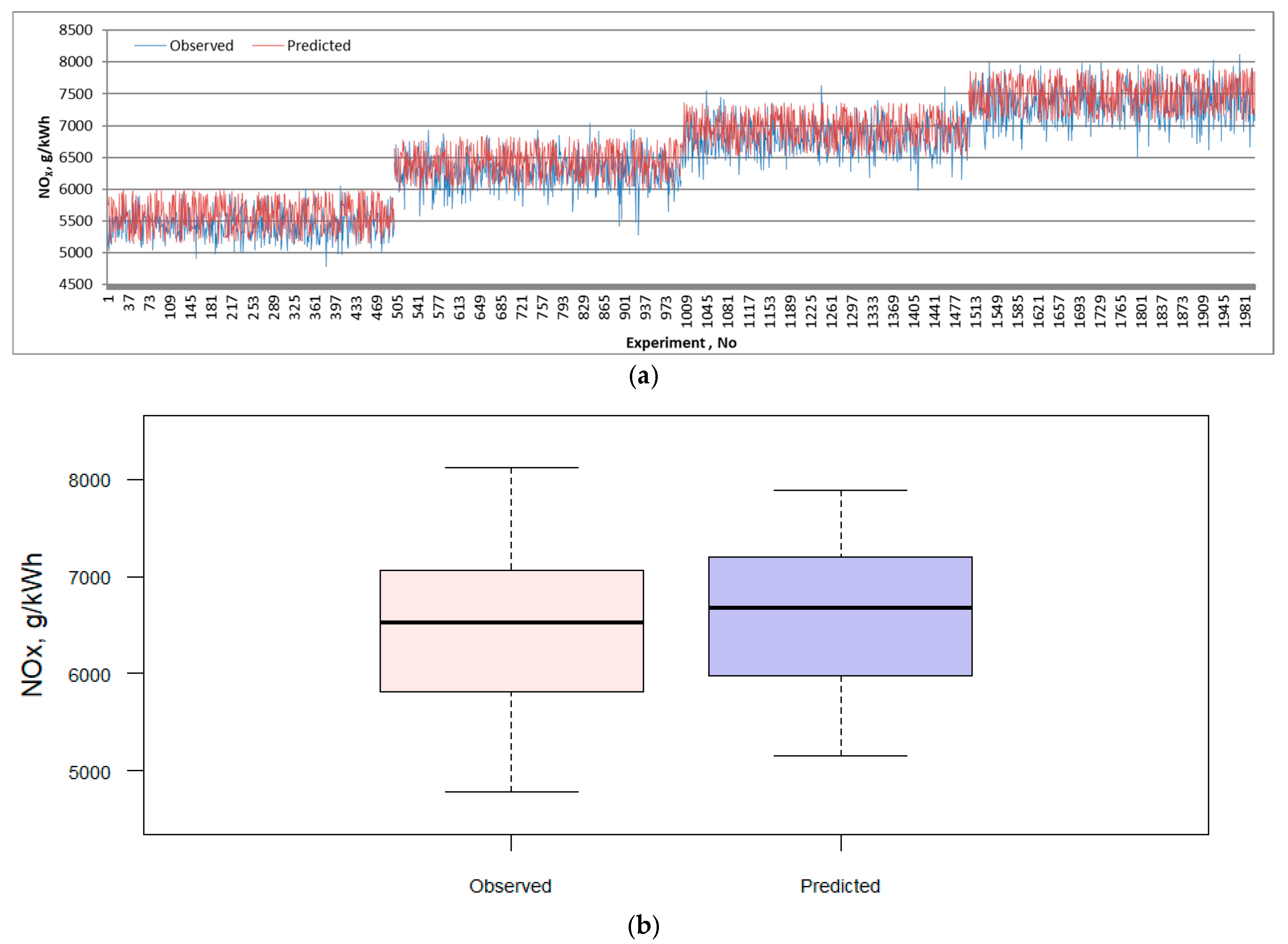
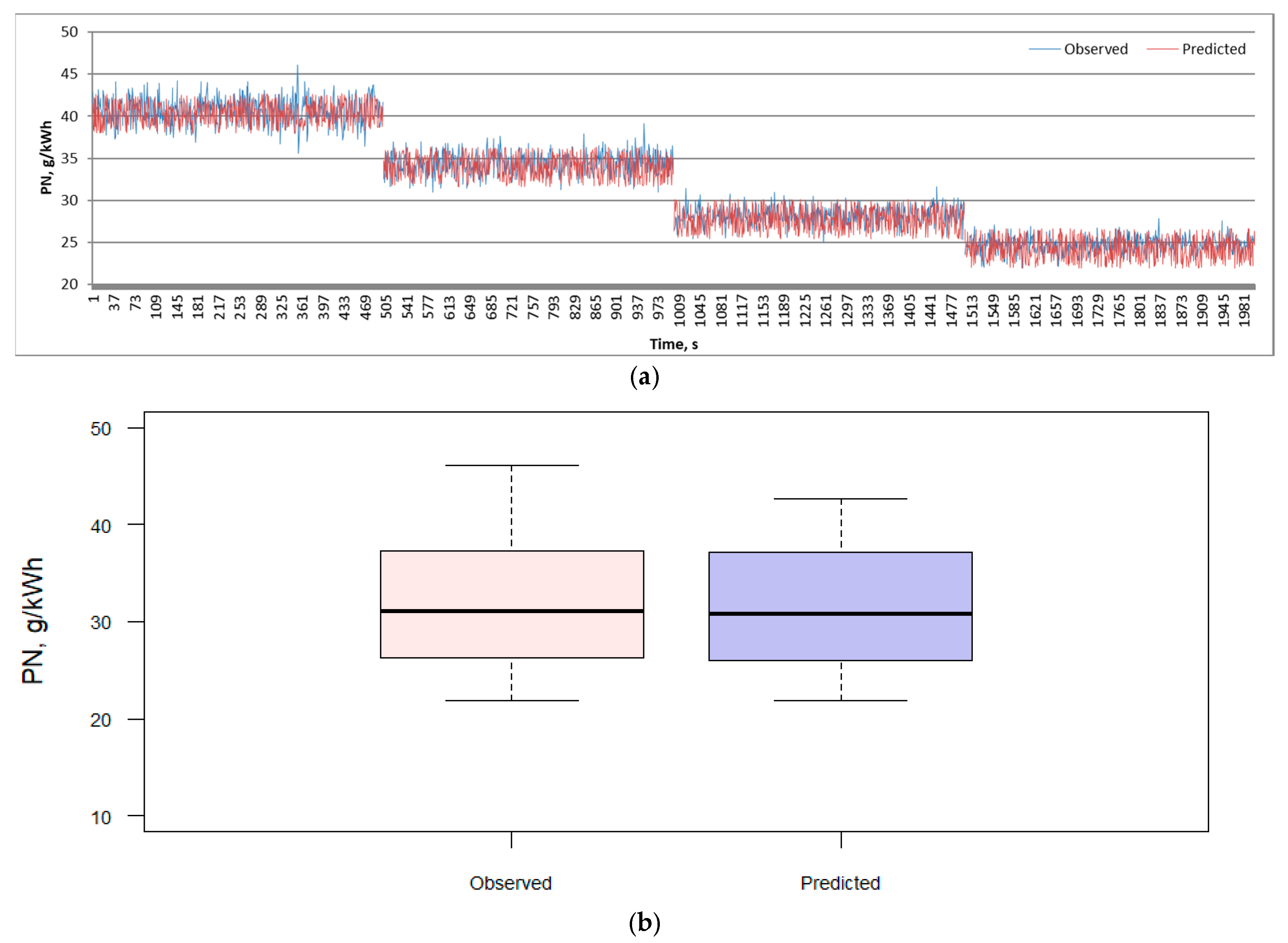
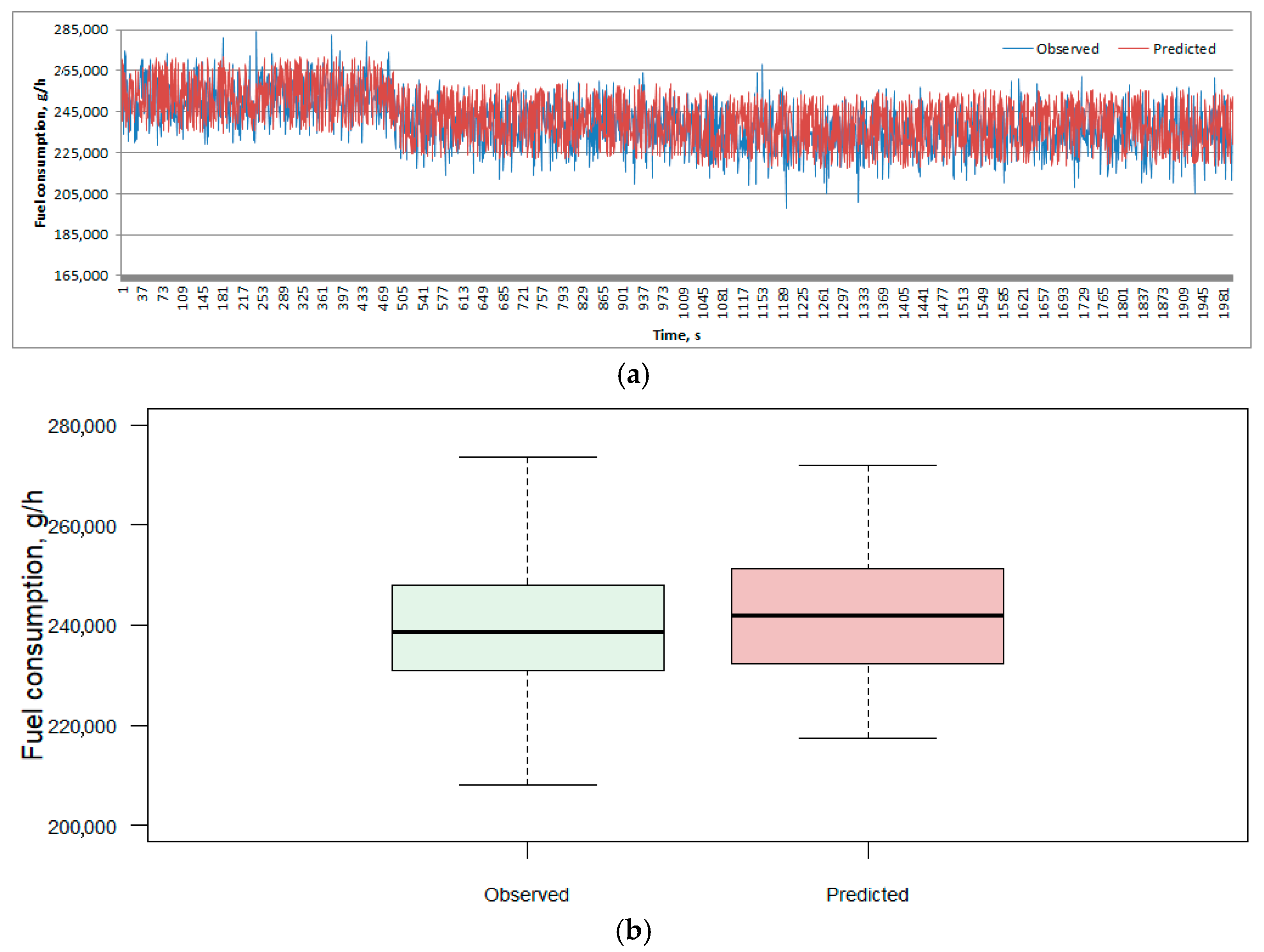
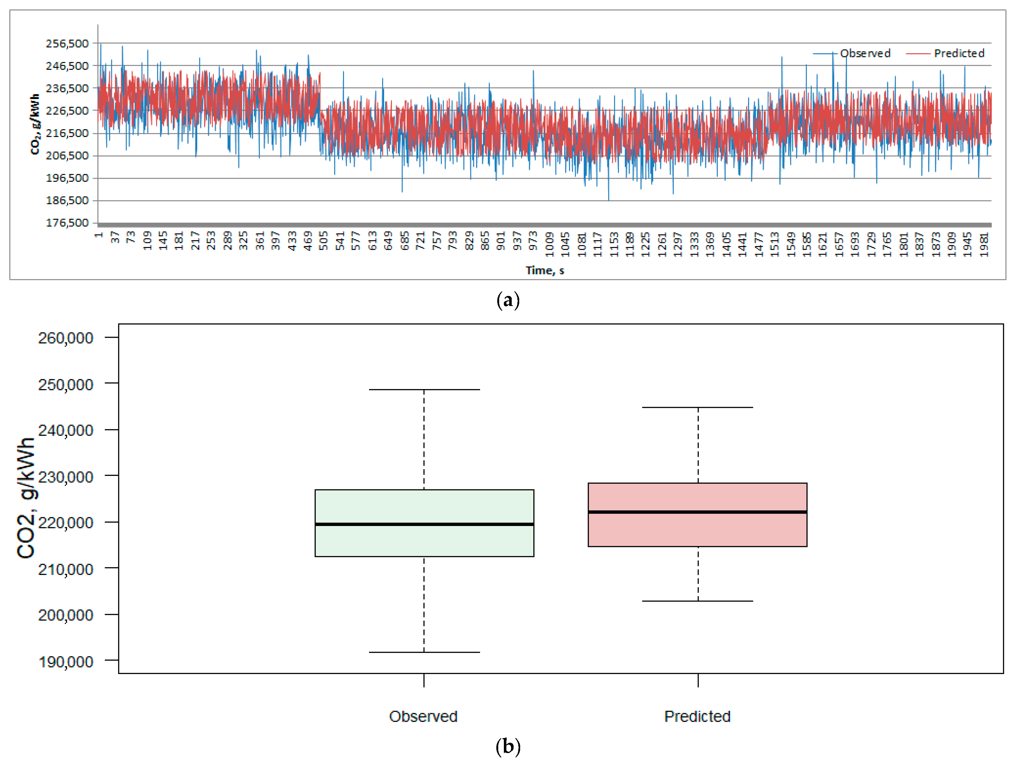
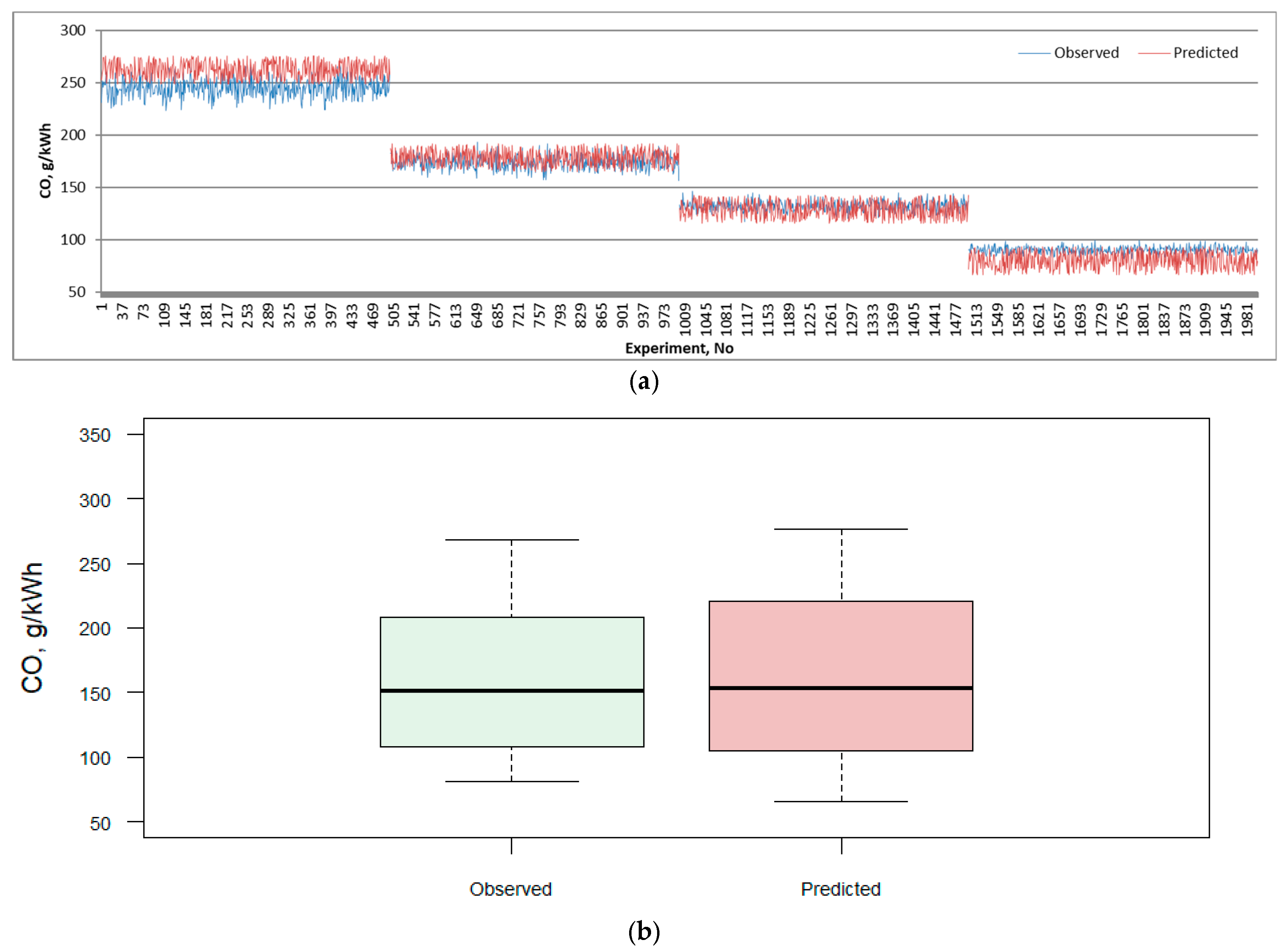
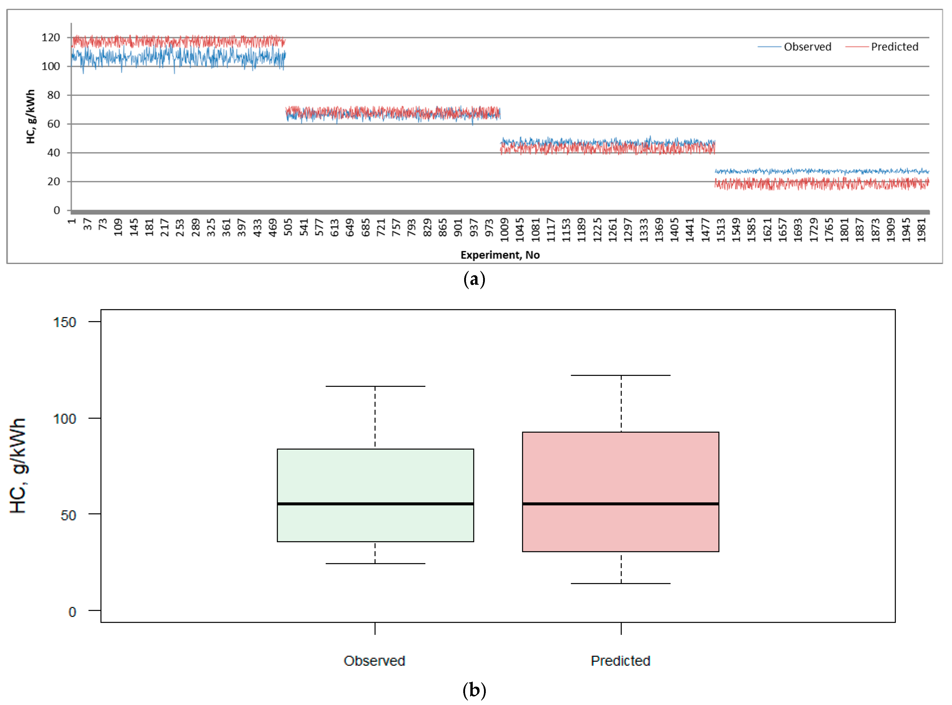
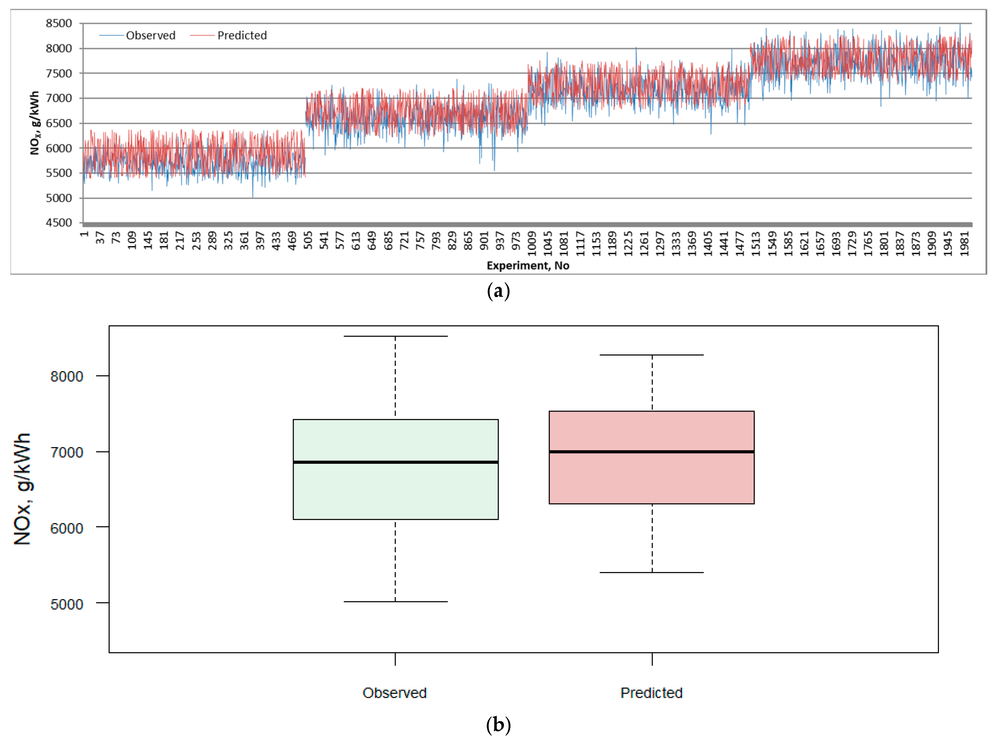
3.2. Model Testing Results

The presented figure (hereinafter referred to as Figure 8) reflects the results of fuel consumption (g/h) prediction when the WCO biodiesel parameters were input into the machine learning (ML) model, which was previously trained on diesel fuel data. These predictions were compared with real experimental data obtained when the engine was operating on WCO fuel. Such an analysis allows us to assess the transferability of the model between the two different fuels and to identify the main differences in the combustion process.

It can be seen from the figure that the fuel consumption varies from approximately 185,000 g/h to 265,000 g/h. Both the observed (blue line) and predicted (red line) values show a close correlation at most of the experimental points. The overall structure of the data shows a decreasing trend—the consumption gradually decreases from the initial to the last experiments. This may be related to the decreasing load, fuel optimization, or other engine operating parameters.

Most importantly, the ML model, although not trained on WCO fuel, reproduces both long-term and short-term trends in fuel consumption quite accurately. This fact testifies to the generalization ability of the model: even when faced with a non-identical chemical and physical composition of the fuel (WCO has a higher density, lower calorific value, and higher oxygen content), it retains the main dependencies between the input parameters and fuel consumption.

However, some differences are visible: in some places (especially in low-cost areas) the model systematically overestimates consumption values, i.e., predicts higher consumption than was recorded experimentally. This deviation can be explained by the fact that the model has learned the “diesel equivalent”—a fuel with a higher calorific value and lower density—and therefore, when transferred to the WCO context, the model attributes an excessive amount of consumption to the same energy demand. In other words, if the engine actually consumed less WCO due to more optimal combustion (e.g., due to higher cetane number or presence of oxygen), the model could not predict this because it did not “see” this type of combustion during training.

Despite these differences, the overall variance between the actual and predicted values remains small. This indicates that even with a slight increase in the model error due to the fuel change, the model has not lost control—it remains functional, and the prediction error is likely to remain below 5–7% at most points.

This result has important practical implications. First, it allows the application of an ML model trained on diesel as a first step in predicting alternative fuels, reducing the need to repeat expensive experiments for each fuel type. Second, this case shows that the success of the model’s transferability strongly depends on the similarity of fuel properties. Although WCO has a lower calorific value (~37.1 MJ/kg) than diesel (~43.2 MJ/kg), their cetane numbers and densities are close enough that the model is able to partially compensate for the differences.

Figure 9 shows a comparison of carbon dioxide (CO₂) emissions between predicted values obtained from a machine learning (ML) model trained on diesel and actual experimental data obtained from WCO biodiesel. This analysis allows us to assess the universality of the model, the ability to transfer knowledge to the context of alternative fuels, and the sensitivity of CO₂ emissions to fuel origin.

According to the graph, CO₂ emissions vary in the range from ~176,000 g/h to ~256,000 g/h, with their highest concentration observed in the range of ~210,000–240,000 g/h. The data is arranged in a segmented manner, which indicates that the tests were performed at different engine operating points or load modes. This is very important, since CO₂ emissions are strongly correlated with the mass and calorific value of the fuel consumed—both of which change when switching from diesel to WCO.

A significant aspect is that although the model was trained using diesel, it was able to accurately reproduce the CO₂ emission distribution trend. The red prediction curve essentially follows the blue actual line in all operating zones. This shows that the ML model successfully captured the essential relationships between input parameters and CO₂ emissions even when the input fuel parameters (e.g., density, LHV) were specific to WCO and not diesel.

It is important to note that the model, in contrast to the fuel consumption case, slightly overestimates CO₂ emissions in some operating zones. This deviation is based on physics—WCO has a ~14% lower calorific value than diesel, so more fuel is burned to produce the same amount of energy. However, WCO has a lower carbon content per unit mass (~81.2% vs. ~86% in diesel), which means that CO₂ emissions per kilogram of fuel should be lower. An ML model trained only on diesel does not fully “see” this difference and therefore can interpret the CO₂ content as proportional only to the mass of fuel consumed, and not to the total carbon content in the fuel.

On the other hand, the general distribution and jumps in the data reflect the real sensitivity of the combustion process to load changes. Both the predictions and the actual emissions show the same pattern of decrease and increase again when switching between different operating zones, which testifies to the model’s ability to capture systematic, non-random changes.

The model’s ability to predict CO₂ emissions with sufficient accuracy even when switching fuels allows it to be used for transferability assessment and emission scenario development, especially in cases where experimental measurements are not possible or limited. Such models can be integrated into evaluation systems for ship decarbonization strategies, allowing for a quick assessment of how much emissions would be reduced by applying different fuel blends or alternatives.

It is also important to emphasize that CO₂ emissions are a direct function of fuel composition, so knowing the chemical structure of WCO (0.812 mass fraction carbon, 0.117 oxygen) well allows us to predict the expected CO₂ release even analytically. The ability of the ML model to closely replicate this without a direct emission formula confirms its predictive reliability.

Figure 10 presents a comparison of carbon monoxide (CO) emission intensity (g/kWh) between machine learning (ML) model predictions and actual measurement results. The model was trained using diesel fuel data, but its performance is analyzed here when biodiesel derived from used cooking oil (WCO) is input. Such a methodology allows us to assess the model’s ability to generalize beyond the training set and reveal how the dynamics of CO emissions differ when changing the fuel composition.

As the figure shows, the data are arranged into four separate zones, corresponding to different engine operating modes or load levels. In each zone, CO emissions fluctuate in a different range: from ~260 g/kWh in the first zone to ~90 g/kWh in the last. This is typical—CO emissions, as a product of incomplete combustion, are usually higher at low efficiency, uneven combustion conditions, or when there is too much excess air, especially in transient operating modes.

A distinctive feature of this analysis is that the ML model tends to overestimate CO emissions in all operating zones. The red prediction curve is higher than the blue actual line, especially in the first two zones. Such a deviation clearly signals that the model is unable to fully adapt to the changed fuel composition.

One might gain a deeper comprehension of this phenomenon by examining it through a physical lens. The oxygen content of WCO biodiesel is significantly elevated, approximately 11.7% by weight, in comparison to conventional diesel. This enhancement facilitates a more efficient oxidation process of carbon monoxide to carbon dioxide, particularly within the combustion core. Consequently, the carbon monoxide emissions resulting from the combustion of waste cooking oil are less than those produced by diesel fuel when subjected to identical conditions. Since the model was trained only with diesel, in which the oxygen content is almost zero, it cannot estimate this additional oxidation potential, and therefore consistently overpredicts the CO content.

However, it is worth noting that although the absolute accuracy of the model has decreased, it maintains good trend tracking—i.e., it accurately captures when CO emissions increase or decrease with changing operating modes. Furthermore, the prediction bias is relatively constant across zones, suggesting that some compensation factor or retraining could easily bring the model accuracy back to acceptable limits.

These results indicate that the transferability of the model in CO emission prediction is limited without additional adaptations. However, this analysis confirms that WCO biodiesel is cleaner in combustion than diesel—the actual CO emission level in each operating mode is lower, which can significantly contribute to the implementation of emission reduction strategies.

This result also highlights that in some cases, the transferability of ML models is emission-selective: For example, if a model is relatively successful in predicting fuel consumption or CO₂ emissions, this does not mean that it will also accurately predict CO or HC, the amounts of which depend strongly on the chemical composition of the fuel and the kinetics of the combustion reaction.

Figure 11 analyzes the variation in hydrocarbon (HC) emission intensity (g/kWh) when WCO biodiesel parameters were input into a machine learning (ML) model trained on diesel fuel data, and it compares the results with real emissions measured during engine testing with WCO fuel. This analysis allows us to assess the ability of the ML model to predict incomplete combustion products when the chemical composition of the fuel differs from the original training base.

Figure 11 clearly distinguishes four operating zones, where the HC emission intensity consistently decreases—from ~110–120 g/kWh at the beginning to ~25–30 g/kWh in the last zone. This is consistent with the physics of combustion: at lower loads, the combustion process becomes more efficient, and HC—as an indicator of incomplete combustion—decreases. The actual data (blue curve) shows a relatively tight but fluctuating structure, while the predictions (red curve) present a smoother picture with a noticeable systematic deviation.

An observation of notable importance is that the ML model invariably overestimates HC emissions across all operating zones. This is apparent in both the elevated and diminished emission ranges. This systematic error suggests that the diesel-trained model lacks a precise representation of the WCO properties pertinent to the completeness of combustion. The main difference between diesel and WCO is the oxygen content in the fuel (~0% in diesel and ~12% WCO in biodiesel). This oxygen is immediately available in the combustion reaction, so combustion with WCO occurs more cleanly and more efficiently, with a lower amount of incomplete oxidation products—i.e., lower HC emission.

Given that the model has been exclusively trained on diesel, where the efficiency of combustion is significantly influenced by air intake, it is unable to provide accurate predictions for WCO combustion, in which the chemical oxygen present in the fuel plays a crucial role in diminishing hydrocarbon emissions. Consequently, it becomes evident that the forecasts are excessively elevated, particularly within the initial two zones, where HC levels are inherently greater owing to diminished engine efficiency.

This phenomenon is important when assessing the limited transferability of the ML model with respect to HC emissions. On the other hand, the behavior of the predictions still captures the correct trends: as the load decreases or the operating mode changes, HC emissions in the predictions also decrease. This means that the structural components of the model work well, but the result suffers from fuel specifics that were not “seen” by the model during training.

It is also important that the model predictions remain stable—there are no sudden distortions or unexpected spikes, and the variance is close to the spread of the actual data. This shows that the model remains reliable as a first-stage predictor, which could be improved by fine-tuning with a small WCO database.

This case also shows that WCO biodiesel can have clear environmental benefits from a combustion perspective, due to more efficient combustion, lower HC content, and lower odorous and reactive emissions. The need to reprogram the ML model highlights the need to develop fuel-type-sensitive architectural solutions if greater accuracy is to be achieved.

Figure 12 shows the changes in nitrogen oxide (NO_x) emission intensity (g/kWh) when the ML model trained on diesel data was applied to WCO fuel conditions, and the obtained predictions were compared with actual measurements. This analysis allows us to assess the model’s ability to predict NO_x emissions for an alternative fuel type with a higher oxygen content and lower calorific value.

As can be seen in the graph, NO_x emission values are distributed from ~5000 g/kWh to almost 8500 g/kWh, and the emission level gradually increases between operating zones, which indicates different engine loads or speed levels. This emission behavior is typical for internal combustion engines, since the NO_x content is closely related to the combustion temperature and excess oxygen during combustion—both conditions tend to increase with engine load.

The predicted values (red curve) show that the model successfully reflects the general trend of increasing emissions. The shape and dynamics of the curve, including the transitions between zones, are very close to the actual emission course (blue curve), which means that the model has maintained its functional structure even after switching to the new fuel type.

However, one important aspect is worth noting: the model consistently overestimates NO_x emissions almost throughout the work—especially when switching between 7000 and 15,000 experimental points. This overestimation can be explained by the fact that WCO has a higher cetane number (56 vs. 55 in diesel) and an additional oxygen content (~12% by mass), which leads to a faster combustion initiation and slightly lower maximum temperatures. These conditions inhibit NO_x formation, but the model trained on diesel does not estimate this effect.

In addition, the actual emissions show a larger amplitude of oscillations—this is possibly related to experimental conditions, air supply variations, or combustion irregularities, while the model predictions remain more consistent. This effect suggests that the model “smooths out” unexpected peak effects, but this results in some loss of realism at the detailed level.

On the other hand, it is important to note that the model does not have a systematic bias when changing operating zones—it adapts proportionally to changes in each zone. This means that the model architecture was flexible enough to generate accurate relative predictions even when absolute differences are large.

The practical implication of this result is that NO_x predictions using models trained on other fuels may be overestimated, especially when alternative fuels (e.g., WCO) reduce combustion temperatures. This suggests the need to adjust the model’s NO_x emission prediction using additional combustion performance parameters (e.g., ignition delay, EGR ratio, calorific value).

Figure 13 analyzes the dynamics of the change in the intensity of particulate number (PN) emissions (g/kWh) when the model trained on diesel fuel was applied to the WCO biodiesel context. The model predictions (red curve) are compared with the actual PN emission measurements (blue curve) obtained during engine tests using WCO fuel.

The emission data are clearly segmented into four operating zones, which correspond to different engine load regimes. In each zone, a decreasing level of PN emissions is observed—from ~31–32 g/kWh in the first zone to ~18–19 g/kWh in the last. This decrease is consistent and logically justified, since lower load and more efficient combustion conditions reduce the amount of incompletely burned particles.

The most important observation is that the ML model overestimates PN emissions in all operating zones, especially in the first two. The expected values remain consistently higher than the actual measurements, with some discrepancies in specific cases reaching 3–5 g/kWh. This error is of significant consequence, indicating that the model has not been sufficiently customized to address the specific characteristics of the fuel in question. The chemical oxygen concentration (about 12%) of WCO biodiesel enhances fuel oxidation during combustion, minimizing the formation of soot and particulate matter.

Given that the model was created using diesel, an oxygen-free fuel, it lacks the ability to understand this improvement in the internal combustion process. It anticipates the amount of particulate matter that would be produced by diesel combustion at an equivalent air/fuel ratio, despite the cleaner combustion properties of waste cooking oil.

Despite this overestimation tendency, the model maintains the right direction in emission decrease as it transitions from one operational zone to another. This indicates that the functional skeleton of the model is working: when the input data changes (e.g., load decreases, fuel flow), the model reduces the PN prediction accordingly. This is critical for determining the model’s structural stability and potential applicability.

The actual emissions (blue line) show less volatility than predicted, implying that the genuine combustion process under WCO circumstances is more stable. This stability can be attributed to the higher cetane number of WCO (~56), better ignition dynamics, and a homogenized combustion process. Meanwhile, the model was trained with a larger dispersion of diesel emissions, and this is reflected in the predictions—they are “noisier”.

The analysis results show that the transferability of the ML model with respect to PN emissions is limited. This is not surprising, since PN formation is particularly sensitive to fuel chemistry, injector dynamic response, and even injection angle—all of which differ between diesel and WCO. Therefore, to achieve high PN prediction accuracy, it would be necessary to perform a correction or retraining of the model with at least part of the WCO data.

Table 1. Accuracy metrics for trained and tested models.

Emission	RMSE		MAE		MAPE		R2
	Training	Testing	Training	Testing	Training	Testing	Training	Testing
NOx	253.2	270.3	14.2	18.8	7.6	10.6	93.6	91.4
CO2	7.2	10.7	2.3	5.3	7.1	10.2	98.9	91.6
CO	9161.4	9188.8	85.2	89.6	8.0	9.3	906	88.2
HC	3.1	7.2	1.5	3.9	7.0	8.2	99.3	95.3
PN	1.2	4.8	1.0	3.1	7.4	8.6	96.1	91.2
Fuel consumption	9757.2	10,133.5	88.3	113.4	8.5	10.9	93.3	90.5

displays the machine learning model’s accuracy for both training and testing datasets with varying fuel consumption and emission characteristics. The results show that the model consistently performs well, particularly for CO₂, HC, and PN. The testing R² values are over 90%, and the RMSE and MAPE values are reasonably low, which means that the model is good at generalizing.

NO_x estimates are likewise very accurate (R² = 91.4%), even though emissions related to combustion temperature tend to vary more. There are slightly more errors in CO and fuel consumption (for example, CO RMSE = 9189 and fuel consumption RMSE ≈ 10,134). This could be because the model is sensitive to transient regimes and fuel-specific characteristics that were not fully captured during training. Despite these challenges, the model remains robust, with testing R² values of 88%. Overall, the table demonstrates that the model can still make correct predictions for all of the variables examined, even when applied to data it has never encountered before.

4. Discussion

The amount of data, in other words, the number of experiments performed, is critically important for building predictive models. In order to build deep neural predictive models, the amount of data must be extremely large. Tens of thousands of observations are usually used to train a model. Such an amount of data is difficult to achieve in engineering tests. However, there are several ways to solve this problem. One of them is data augmentation, which allows the experiment to be expanded with very similar data. Another way to solve this problem is to use shallow models such as linear regression models or other regression models [59,60].

In order to understand the behavior of the combustion process, the interdependence of emissions and the relationship between fuel consumption and pollutant emissions, a pairwise correlation analysis was performed between the main emission parameters (NO_x, CO₂, CO, HC, PN) and fuel consumption (see Figure 14). This analysis includes three different fuel cases: diesel (red), WCO biodiesel (blue) and both fuels (green). The Pearson correlation coefficient, visualized data density functions, and scatter plots were used for the evaluation [61,62].

Nitrogen oxides (NO_x) emissions are negatively correlated with CO₂ emissions for both diesel (r = −0.336) and both fuels (−0.363). This reflects the well-known trade-off between efficient combustion and NO_x emissions—as combustion efficiency increases (when CO₂ increases), NO_x decreases—since more efficient combustion is often associated with lower temperatures or more optimal combustion times.

Meanwhile, the correlation between NO_x and CO emissions is strongly negative (r ≈ −0.933 in all cases), which indicates opposite emission formation conditions: NO_x increases at high temperatures and good oxygen supply, and CO decreases when combustion is incomplete. The substantial negative correlation between NO_x and HC (r = −0.931) suggests that combustion quality has a systematic effect on pollutant distribution.

The connection between NO_x and fuel consumption is moderately negative (r = −0.355), indicating that greater combustion efficiency leads to decreased NO_x levels. In the case of WCO, the correlations weaken but remain with the same sign.

CO₂, as a product of complete combustion, naturally correlates positively with indicators of incomplete combustion—CO (r = 0.388) and HC (r = 0.405). This relationship is strongest for diesel, but it also persists in the blend. This reflects the fact that more efficient combustion leads to higher CO₂ emissions, but lower emissions of other pollutants—soot, CO, and HC.

The correlation between CO₂ and fuel consumption is weakly positive (r = 0.169–0.287), which is understandable, since higher consumption essentially means more fuel burned, and therefore more CO₂ released. However, the low strength of the correlation indicates that the variation in CO₂ emissions depends more on the quality of the combustion process than on the mass of the fuel alone.

CO emissions show a very strong correlation with HC (r = 0.990 in both fuels, 0.989 for WCO). This is natural, since both pollutants are formed as a result of incomplete combustion—one as a partial combustion product, the other as unbroken hydrocarbons. In addition, CO emissions are also closely related to PN emissions (r ≈ 0.849), as incomplete combustion also leads to soot formation.

CO and fuel consumption are positively correlated (r = 0.372–0.528), especially for diesel and both fuels. This indicates that higher consumption is usually associated with lower combustion efficiency, when more fuel evaporates due to incomplete combustion. In the case of WCO, this relationship remains, but somewhat weaker, which can be explained by a better combustion balance of biodiesel due to the oxygen content in the fuel.

Hydrocarbon emissions, including CO, are strongly correlated with PN (r ≈ 0.968) and fuel consumption (r = 0.372–0.540). This demonstrates the overall relationship between combustion inefficiency and pollution: when the fuel combination combusts unevenly or under less-than-ideal conditions, hydrocarbons, soot, and CO emissions increase.

In both fuels, there is a stronger link between HC and fuel consumption compared to CO₂. Although CO₂ emissions may decrease with lower carbon content, the strong correlation between HC and consumption remains, possibly due to higher fuel flow needs.

PN shows a moderate to strong correlation with all incomplete combustion indicators: CO, HC (r ≈ 0.849–0.968), and fuel consumption (r = 0.063–0.518). This suggests that PN is a consequence of complex combustion inefficiency. In the case of WCO and both fuels, these correlations are somewhat weaker, which can be explained by the fact that the higher oxygen content in the fuel improves the oxidation of particles during combustion.

The consumption of fuel exhibits a robust positive correlation with all pollutants, with the exception of NO_x. This is particularly apparent in the instances of CO (r = 0.528), HC (r = 0.540), and PN (r = 0.518), which can be rationalized by the fact that heightened fuel consumption results in an increase in pollutants, particularly when the combustion process is not finely tuned. The optimization of combustion processes, especially when utilizing WCO as fuel, leads to a decrease in NO_x emissions, evidenced by the inverse relationship with fuel consumption.

5. Conclusions

The machine learning model, developed with diesel data, demonstrated a commendable level of prediction accuracy concerning fuel consumption and critical emission parameters (NO_x, CO₂, CO, HC, PN) across diverse engine operating modes. The findings validate the appropriateness of this model for the real-time monitoring and regulation of emissions in marine internal combustion engines.

By introducing WCO biodiesel parameters into the same model, the consistency of emission dynamics prediction was maintained, despite differences in fuel composition. This showed that the model is partially able to adapt to alternative fuels without additional retraining.

The observed systematic overestimation of CO, HC, and PN emissions in the WCO mode revealed the limitations of the model when applying it to fuels with a higher oxygen content. The differences are because the model cannot take into account the better combustion quality that comes from the higher cetane number and oxygen concentration in the WCO mixture.

Even though there were certain biases, the model’s predictions always showed the right path for changes in emissions in relation to changes in load. This allows us to conclude that a small retraining (fine-tuning) with WCO data could significantly increase the accuracy of the predictions.

Pairwise correlation analysis revealed strong relationships between incomplete combustion emissions (CO, HC, PN) and their dependence on fuel consumption. Meanwhile, NO_x emissions showed a negative correlation with CO₂ and consumption, which reflects the classic efficiency–pollution trade-off.

The results confirm that ML models are an effective tool for emission prediction, fuel analysis, and mixed operation modeling, allowing for early assessment of the impact of alternative fuels without extensive experimental testing. Such models increase the flexibility and sustainability of engine research in marine engineering.

Future endeavors may concentrate on incorporating dynamic engine performance variables such as torque and effective power into the model’s functionalities. The significance of these factors lies in their role in assessing the efficacy of the propulsion system and its responsiveness to loads in real-time scenarios. Should additional operational parameters be accessible through onboard sensors or simulation inputs, the existing model architecture can be adapted accordingly to accommodate this requirement.

References

1. Sun, Z.; Zhang, W.; Nour, M.; Li, X.; Hung, D.L.S.; Xu, M. Interaction Mechanisms of Flash Boiling Spray with Air-Wall-Time in a SIDI Engine and Implications on Flame Propagation and Emissions Using Experimental Investigation and Machine Learning. Energy 2025, 328, 136633. [Google Scholar] [CrossRef]
2. Mlynski, R.; Kozlowski, E. Selection of Level-Dependent Hearing Protectors for Use in An Indoor Shooting Range. Int. J. Environ. Res. Public Health 2019, 16, 2266. [Google Scholar] [CrossRef]
3. Jovanović, V.; Janošević, D.; Marinković, D.; Petrović, N.; Djokić, R. Analysis of Influential Parameters in the Dynamic Loading and Stability of the Swing Drive in Hydraulic Excavators. Machines 2024, 12, 737. [Google Scholar] [CrossRef]
4. Gu, J.; Wang, Y.; Hu, J.; Zhang, K.; Shi, L.; Deng, K. Real-Time Prediction of Fuel Consumption and Emissions Based on Deep Autoencoding Support Vector Regression for Cylinder Pressure-Based Feedback Control of Marine Diesel Engines. Energy 2024, 300, 131570. [Google Scholar] [CrossRef]
5. Borucka, A.; Kozlowski, E. Mathematical Evaluation of Passenger and Freight Rail Transport as Viewed Through the COVID-19 Pandemic and the War in Ukraine Situation. Adv. Sci. Technol.-Res. J. 2024, 18, 238–249. [Google Scholar] [CrossRef]
6. Žvirblis, T.; Vainorius, D.; Matijošius, J.; Kilikevičienė, K.; Rimkus, A.; Bereczky, Á.; Lukács, K.; Kilikevičius, A. Engine Vibration Data Increases Prognosis Accuracy on Emission Loads: A Novel Statistical Regressions Algorithm Approach for Vibration Analysis in Time Domain. Symmetry 2021, 13, 1234. [Google Scholar] [CrossRef]
7. Odufuwa, O.Y.; Tartibu, L.K.; Kusakana, K. Artificial Neural Network Modelling for Predicting Efficiency and Emissions in Mini-Diesel Engines: Key Performance Indicators and Environmental Impact Analysis. Fuel 2025, 387, 134294. [Google Scholar] [CrossRef]
8. Kumar, V.; Choudhary, A.K. Prediction of the Performance and Emission Characteristics of Diesel Engine Using Diphenylamine Antioxidant and Ceria Nanoparticle Additives with Biodiesel Based on Machine Learning. Energy 2024, 301, 131746. [Google Scholar] [CrossRef]
9. Zhang, J.; Li, X.; Amini, M.R.; Kolmanovsky, I.; Tsutsumi, M.; Nakada, H. Modeling and Control of Diesel Engine Emissions Using Multi-Layer Neural Networks and Economic Model Predictive Control. IFAC-Pap. 2023, 56, 10696–10702. [Google Scholar] [CrossRef]
10. Rohani, A.; Zareei, J.; Ghadamkheir, K.; Farkhondeh, S.A. Optimization of Engine Parameters and Emission Profiles through Bio-Additives: Insights from ANFIS Modeling of Diesel Combustion. Clean. Eng. Technol. 2025, 27, 100994. [Google Scholar] [CrossRef]
11. Liu, L.; Shao, W.; Yan, Y.; Liu, D.; Zhang, J. Intelligent Self-Adaption of Marine Engine Degradation Based on a Digital-Twin Model. Energy Convers. Manag. 2025, 341, 119995. [Google Scholar] [CrossRef]
12. Dişlitaş, A.N.; Yıldız, M.; Kale-Halasz, G. Digital Twin Applications in Aircraft Design Process. In Proceedings of the 3rd Cognitive Mobility Conference, Budapest, Hungary, 7–8 October 2024; Zöldy, M., Ed.; Lecture Notes in Networks and Systems. Springer Nature: Cham, Switzerland, 2025; Volume 1258, pp. 436–444, ISBN 978-3-031-81798-4. [Google Scholar]
13. Gökçe, C.; Yıldız, M.; Kale-Halasz, G. VTOL Craft Controller Design and Simulation Using Digital Twin. In Proceedings of the 3rd Cognitive Mobility Conference, Budapest, Hungary, 7–8 October 2024; Zöldy, M., Ed.; Lecture Notes in Networks and Systems. Springer Nature: Cham, Switzerland, 2025; Volume 1258, pp. 401–413, ISBN 978-3-031-81798-4. [Google Scholar]
14. Imanov, T.; Yildiz, M.; Teimourian, H.; Matijošius, J.; Kale, U.; Kilikevičius, A. 1D Convolutional Neural Networks Application on Aircraft Engine Thermal Performance Parameters. J. Therm. Anal. Calorim. 2025. [Google Scholar] [CrossRef]
15. Park, M.-H.; Hur, J.-J.; Lee, W.-J. Prediction of Diesel Generator Performance and Emissions Using Minimal Sensor Data and Analysis of Advanced Machine Learning Techniques. J. Ocean. Eng. Sci. 2025, 10, 150–168. [Google Scholar] [CrossRef]
16. Pallicheruvu, N.K.; Gnanasekaran, S. ANN-Driven Prediction of Optimal Machine Learning Models for Engine Performance in a Dual-Fuel Mode Powered by Biogas and Fish Oil Biodiesel. Energy Convers. Manag. X 2025, 25, 100827. [Google Scholar] [CrossRef]
17. Dewang, Y.; Sharma, V.; Singla, Y.K. A Critical Review of Waste Tire Pyrolysis for Diesel Engines: Technologies, Challenges, and Future Prospects. Sustain. Mater. Technol. 2025, 43, e01291. [Google Scholar] [CrossRef]
18. Oloruntobi, O.; Mokhtar, K.; Himawan, A.F.I.; Gohari, A.; Onigbara, V.; Rozar, N.; Balasudarsun, N.L. Economic and Environmental Assessment of Fatty-Acid-Methyl-Ester and Hydrotreated Vegetable Oil Biofuels Viability for Future Marine Engines. Bioresour. Technol. Rep. 2025, 30, 102146. [Google Scholar] [CrossRef]
19. Wang, K.; Chi, Y.; Liang, H.; Jing, Z.; Li, Z.; Ma, R.; Huang, L. Carbon Emission Monitoring and Control Technology for Ships: A Review. Mar. Pollut. Bull. 2025, 219, 118219. [Google Scholar] [CrossRef]
20. Li, Z.; Fei, J.; Du, Y.; Ong, K.-L.; Arisian, S. A near Real-Time Carbon Accounting Framework for the Decarbonization of Maritime Transport. Transp. Res. Part E: Logist. Transp. Rev. 2024, 191, 103724. [Google Scholar] [CrossRef]
21. Marashian, A.; Böling, J.M.; Razminia, A.; Hyvönen, J.; Vettor, R.; Gustafsson, W.; Pirttikangas, M.; Björkqvist, J. Combined Engine Configuration and Speed Optimization for Fuel Savings on Cruise Ships. Ocean Eng. 2025, 322, 120387. [Google Scholar] [CrossRef]
22. Mitchell, T.M. Machine Learning; McGraw-Hill Series in Computer Science; McGraw-Hill: New York, NY, USA, 1997; ISBN 978-0-07-042807-2. [Google Scholar]
23. Alahmer, H.; Alahmer, A.; Alkhazaleh, R.; Al-Amayreh, M.I. Modeling, Polynomial Regression, and Artificial Bee Colony Optimization of SI Engine Performance Improvement Powered by Acetone–Gasoline Fuel Blends. Energy Rep. 2023, 9, 55–64. [Google Scholar] [CrossRef]
24. Cohen, J.; Cohen, J. Applied Multiple Regression/Correlation Analysis for the Behavioral Sciences; L. Erlbaum Associates: Mahwah, NJ, USA, 2003; ISBN 978-1-4106-0626-6. [Google Scholar]
25. Kozłowski, E.; Antosz, K.; Sęp, J.; Prucnal, S. Integrating Sensor Systems and Signal Processing for Sustainable Production: Analysis of Cutting Tool Condition. Electronics 2023, 13, 185. [Google Scholar] [CrossRef]
26. Borucka, A.; Kozłowski, E. Modeling the Dynamics of Changes in CO2 Emissions from Polish Road Transport in the Context of COVID-19 and Decarbonization Requirements. Combust. Engines 2023, 195, 63–70. [Google Scholar] [CrossRef]
27. Surblys, V.; Kozłowski, E.; Matijošius, J.; Gołda, P.; Laskowska, A.; Kilikevičius, A. Accelerometer-Based Pavement Classification for Vehicle Dynamics Analysis Using Neural Networks. Appl. Sci. 2024, 14, 10027. [Google Scholar] [CrossRef]
28. Maritime Ships Database. Available online: https://directory.marinelink.com/ships/ (accessed on 20 June 2025).
29. Chiavola, O.; Matijošius, J.; Palmieri, F.; Recco, E. Engine and Emission Performance of Renewable Fuels in a Small Displacement Turbocharged Diesel Engine. Energies 2024, 17, 6443. [Google Scholar] [CrossRef]
30. Chiatti, G.; Chiavola, O.; Palmieri, F. Vibration and Acoustic Characteristics of a City-Car Engine Fueled with Biodiesel Blends. Appl. Energy 2017, 185, 664–670. [Google Scholar] [CrossRef]
31. Rimkus, A.; Žaglinskis, J.; Stravinskas, S.; Rapalis, P.; Matijošius, J.; Bereczky, Á. Research on the Combustion, Energy and Emission Parameters of Various Concentration Blends of Hydrotreated Vegetable Oil Biofuel and Diesel Fuel in a Compression-Ignition Engine. Energies 2019, 12, 2978. [Google Scholar] [CrossRef]
32. Elkelawy, M.; El Shenawy, E.A.; Bastawissi, H.A.E.; El Shennawy, I.A. The Effect of Using the WCO Biodiesel as an Alternative Fuel in Compression Ignition Diesel Engine on Performance and Emissions Characteristics. J. Phys. Conf. Ser. 2022, 2299, 012023. [Google Scholar] [CrossRef]
33. Rocha-Meneses, L.; Hari, A.; Inayat, A.; Yousef, L.A.; Alarab, S.; Abdallah, M.; Shanableh, A.; Ghenai, C.; Shanmugam, S.; Kikas, T. Recent Advances on Biodiesel Production from Waste Cooking Oil (WCO): A Review of Reactors, Catalysts, and Optimization Techniques Impacting the Production. Fuel 2023, 348, 128514. [Google Scholar] [CrossRef]
34. Milojević, S.; Stopka, O.; Kontrec, N.; Orynycz, O.; Hlatká, M.; Radojković, M.; Stojanović, B. Analytical Characterization of Thermal Efficiency and Emissions from a Diesel Engine Using Diesel and Biodiesel and Its Significance for Logistics Management. Processes 2025, 13, 2124. [Google Scholar] [CrossRef]
35. Chiavola, O.; Matijošius, J.; Palmieri, F.; Recco, E. Effects of Renewable Fuels on the Performance and Emissions of a Small Displacement Diesel Engine for Urban Mobility; SAE International: Turin, Italy, 2024; Paper Numbers: 2024-37-0019. [Google Scholar]
36. Jain, S.; Chandrappa, A.K. A Laboratory Investigation on Benefits of WCO Utilisation in Asphalt with High Recycled Asphalt Content: Emphasis on Rejuvenation and Aging. Int. J. Pavement Eng. 2023, 24, 2172577. [Google Scholar] [CrossRef]
37. Foo, W.H.; Koay, S.S.N.; Chia, S.R.; Chia, W.Y.; Tang, D.Y.Y.; Nomanbhay, S.; Chew, K.W. Recent Advances in the Conversion of Waste Cooking Oil into Value-Added Products: A Review. Fuel 2022, 324, 124539. [Google Scholar] [CrossRef]
38. Suardi, S.; Setiawan, W.; Nugraha, A.M.; Alamsyah, A.; Ikhwani, R.J. Evaluation of Diesel Engine Performance Using Biodiesel from Cooking Oil Waste (WCO). J. Ris. Teknol. Pencegah. Pencemaran Ind. 2023, 14, 29–39. [Google Scholar] [CrossRef]
39. Outili, N.; Kerras, H.; Meniai, A.H. Recent Conventional and Non-Conventional WCO Pretreatment Methods: Implementation of Green Chemistry Principles and Metrics. Curr. Opin. Green Sustain. Chem. 2023, 41, 100794. [Google Scholar] [CrossRef]
40. Chiavola, O.; Palmieri, F.; Cavallo, D.M. On the Increase in the Renewable Fraction in Diesel Blends Using Aviation Fuel in a Common Rail Engine. Energies 2023, 16, 4624. [Google Scholar] [CrossRef]
41. Liao, J.; Hu, J.; Yan, F.; Chen, P.; Zhu, L.; Zhou, Q.; Xu, H.; Li, J. A Comparative Investigation of Advanced Machine Learning Methods for Predicting Transient Emission Characteristic of Diesel Engine. Fuel 2023, 350, 128767. [Google Scholar] [CrossRef]
42. Gubarevych, O.; Wierzbicki, S.; Melnyk, O.; Kyrychenko, O.; Riashchenko, O. Increasing the acIncreasing the Accuracy of Calculated Indicators of Operational Reliability of Industrial Electric Motorscuracy of Calculated Indicators of Operational Reliability of Industrial Electric Motors. Eksploat. I Niezawodn. Maint. Reliab. 2025, 27, 203006. [Google Scholar] [CrossRef]
43. Vrublevskyi, O.; Wierzbicki, S. Analysis of Potential Improvements in the Performance of Solenoid Injectors in Diesel Engines. Eksploat. I Niezawodn. Maint. Reliab. 2023, 25, 166493. [Google Scholar] [CrossRef]
44. Schwarm, K.K.; Spearrin, R.M. Real-Time FPGA-Based Laser Absorption Spectroscopy Using on-Chip Machine Learning for 10 kHz Intra-Cycle Emissions Sensing towards Adaptive Reciprocating Engines. Appl. Energy Combust. Sci. 2023, 16, 100231. [Google Scholar] [CrossRef]
45. Şahin, S. Comparison of Machine Learning Algorithms for Predicting Diesel/Biodiesel/Iso-Pentanol Blend Engine Performance and Emissions. Heliyon 2023, 9, e21365. [Google Scholar] [CrossRef] [PubMed]
46. Khac, H.N.; Modabberian, A.; Zenger, K.; Niskanen, K.; West, A.; Zhang, Y.; Silvola, E.; Lendormy, E.; Storm, X.; Mikulski, M. Machine Learning Methods for Emissions Prediction in Combustion Engines with Multiple Cylinders. IFAC-Pap. 2023, 56, 3072–3078. [Google Scholar] [CrossRef]
47. Aygun, H.; Dursun, O.O.; Toraman, S. Machine Learning Based Approach for Forecasting Emission Parameters of Mixed Flow Turbofan Engine at High Power Modes. Energy 2023, 271, 127026. [Google Scholar] [CrossRef]
48. Zandie, M.; Ng, H.K.; Gan, S.; Muhamad Said, M.F.; Cheng, X. Multi-Input Multi-Output Machine Learning Predictive Model for Engine Performance and Stability, Emissions, Combustion and Ignition Characteristics of Diesel-Biodiesel-Gasoline Blends. Energy 2023, 262, 125425. [Google Scholar] [CrossRef]
49. Khurana, S.; Saxena, S.; Jain, S.; Dixit, A. Predictive Modeling of Engine Emissions Using Machine Learning: A Review. Mater. Today Proc. 2021, 38, 280–284. [Google Scholar] [CrossRef]
50. Li, B.; Ding, Y.; Ma, W.; Xiang, L.; Sui, C. A Health Condition Assessment Method for Marine Diesel Engine Turbochargers Using Zero-Dimensional Engine Model and Machine Learning. Measurement 2025, 251, 117283. [Google Scholar] [CrossRef]
51. Zhang, Z.; Liang, K.; Pan, M.; Wang, H.; Sang, H.; Zhou, S.; Zhang, S.; Guan, W. Exhaust Emissions Prediction in Spark Ignition Engine Using LightGBM Optimized with the Marine Predators Algorithm. Appl. Therm. Eng. 2025, 275, 126800. [Google Scholar] [CrossRef]
52. Lu, X.; Zhao, J.; Markov, V.; Grekhov, L. Deep Transfer Learning-Based Model for Real-Time Prediction of Multiple Injection Rate in Common Rail System for Marine Engine. Energy 2025, 332, 137206. [Google Scholar] [CrossRef]
53. Saqib, S.; Usman, M.; Shah, A.N.; Riaz, F. A Review of the Utilization of Alternative Sources, Machine Learning, and Optimization Techniques for Spark Ignition Engines: Current Progress and Future Outlook. Results Eng. 2025, 26, 105265. [Google Scholar] [CrossRef]
54. Wang, Y.; Chen, G.; Wang, G.; Qian, D.; Shen, L. Integrated Machine Learning-Based Intelligent Optimization for Clean and Efficient Operation of Diesel Engines and Diesel Particulate Filters in Dual Modes. Process Saf. Environ. Prot. 2025, 201, 107457. [Google Scholar] [CrossRef]
55. Mikulski, M.; Hunicz, J.; Duda, K.; Kazimierski, P.; Suchocki, T.; Rybak, A. Tyre Pyrolytic Oil Fuel Blends in a Modern Compression Ignition Engine: A Comprehensive Combustion and Emissions Analysis. Fuel 2022, 320, 123869. [Google Scholar] [CrossRef]
56. Yuksel, O.; Bayraktar, M.; Sokukcu, M. Comparative Study of Machine Learning Techniques to Predict Fuel Consumption of a Marine Diesel Engine. Ocean. Eng. 2023, 286, 115505. [Google Scholar] [CrossRef]
57. Tang, Y.; Zhao, X.; Feng, J.; Bai, S.; Li, G.; Duan, H.; Zhu, S. Challenges and Opportunities of Natural Gas Dual-Fuel Engines for Marine Applications. Fuel 2025, 400, 135808. [Google Scholar] [CrossRef]
58. Al Nuaimi, H.S.; Acquaye, A.; Mayyas, A. Machine Learning Applications for Carbon Emission Estimation. Resour. Conserv. Recycl. Adv. 2025, 27, 200263. [Google Scholar] [CrossRef]
59. Aggarwal, C. Recurrent Neural Networks. In Neural Networks and Deep Learning: A Textbook; Aggarwal, C.C., Ed.; Springer International Publishing: Cham, Switzerland, 2023; pp. 265–304. ISBN 978-3-031-29642-0. [Google Scholar]
60. Carrington, A.M.; Fieguth, P.W.; Qazi, H.; Holzinger, A.; Chen, H.H.; Mayr, F.; Manuel, D.G. A New Concordant Partial AUC and Partial c Statistic for Imbalanced Data in the Evaluation of Machine Learning Algorithms. BMC Med. Inf. Decis. Mak. 2020, 20, 4. [Google Scholar] [CrossRef] [PubMed]
61. Matijošius, J.; Rimkus, A.; Gruodis, A. Validation Challenges in Data for Different Diesel Engine Performance Regimes Utilising HVO Fuel: A Study on the Application of Artificial Neural Networks for Emissions Prediction. Machines 2024, 12, 279. [Google Scholar] [CrossRef]
62. Matijošius, J.; Rimkus, A.; Gruodis, A. Prediction of the Main Environmental and Energy Characteristics of Diesel Engines Using an Artificial Neural Network for Pure Diesel Fuel, Pure Hvo, and a Mixture OF These Fuels in The Ratio 50/50 by Volume. Transp. Probl. 2024, 19, 69–82. [Google Scholar] [CrossRef]
Figure 1. Test bench diagram: real-time emissions and fuel consumption measurement system on a ferry with VOLVO PENTA D16-MH engines.
Jmse 13 01328 g001
Figure 2. Comparison of fuel consumption (g/h) predictions and actual values using ML model (diesel fuel): (a) observed values compared with regression model, (b) aggregated boxplot distribution for observed and predicted values.
Jmse 13 01328 g002
Figure 3. Comparison of predicted and actual values of CO2 emissions (g/kWh) in different operating modes using the ML model (diesel fuel): (a) observed values compared with regression model, (b) aggregated boxplot distribution for observed and predicted values.
Jmse 13 01328 g003
Figure 4. Comparison of predicted and actual values of CO emissions (g/kWh) in different operating modes using the ML model (diesel fuel): (a) observed values compared with regression model, (b) aggregated boxplot distribution for observed and predicted values.
Jmse 13 01328 g004
Figure 5. Comparison of predicted and actual values of HC emissions (g/kWh) in different operating modes using the ML model (diesel fuel): (a) observed values compared with regression model, (b) aggregated boxplot distribution for observed and predicted values.
Jmse 13 01328 g005
Figure 6. Comparison of predicted and actual values of NOx emissions (g/kWh) in different operating modes using the ML model (diesel fuel): (a) observed values compared with regression model, (b) aggregated boxplot distribution for observed and predicted values.
Jmse 13 01328 g006
Figure 7. Comparison of predicted and actual values of PN emissions (g/kWh) in different operating modes using the ML model (diesel fuel): (a) observed values compared with regression model, (b) aggregated boxplot distribution for observed and predicted values.
Jmse 13 01328 g007
Figure 8. Fuel consumption (g/h) predictions obtained by inputting WCO parameters into a model trained with diesel and comparing with experimental WCO data: (a) observed values compared with regression model, (b) aggregated boxplot distribution for observed and predicted values.
Jmse 13 01328 g008
Figure 9. CO2 (g/kWh) predictions obtained by inputting WCO parameters into a model trained with diesel and comparing with experimental WCO data: (a) observed values compared with regression model, (b) aggregated boxplot distribution for observed and predicted values.
Jmse 13 01328 g009
Figure 10. CO (g/kWh) predictions obtained by inputting WCO parameters into a model trained with diesel and comparing with experimental WCO data: (a) observed values compared with regression model, (b) aggregated boxplot distribution for observed and predicted values.
Jmse 13 01328 g010
Figure 11. HC (g/kWh) predictions obtained by inputting WCO parameters into a model trained with diesel and comparing with experimental WCO data: (a) observed values compared with regression model, (b) aggregated boxplot distribution for observed and predicted values.
Jmse 13 01328 g011
Figure 12. NOx (g/kWh) predictions obtained by inputting WCO parameters into a model trained with diesel and comparing with experimental WCO data: (a) observed values compared with regression model, (b) aggregated boxplot distribution for observed and predicted values.
Jmse 13 01328 g012
Figure 13. PN (g/kWh) predictions obtained by inputting WCO parameters into a model trained with diesel and comparing with experimental WCO data: (a) observed values compared with regression model, (b) aggregated boxplot distribution for observed and predicted values.
Jmse 13 01328 g013
Figure 14. Correlation matrix between emission parameters and fuel consumption, analyzing diesel, WCO, and blended fuel cases. Respectively, black, red, and turquoise color represents whole, diesel, and mixture dataset correlation coefficients and data distribution; *** defines statistically significant correlation coefficient (p < 0.05).
Jmse 13 01328 g014