Influence of Geometric Effects on Dynamic Stall in Darrieus-Type Vertical-Axis Wind Turbines for Offshore Renewable Applications

Abstract

The offshore implementation of vertical-axis wind turbines (VAWTs) presents a promising new paradigm for advancing marine wind energy utilization, owing to their omnidirectional wind acceptance, compact structural design, and potential for lower maintenance costs. However, VAWTs still face major aerodynamic challenges, particularly due to the pitching motion, where the angle of attack varies cyclically with the blade azimuth. This leads to strong unsteady effects and susceptibility to dynamic stalls, which significantly degrade aerodynamic performance. To address these unresolved issues, this study conducts a comprehensive investigation into the dynamic stall behavior and wake vortex evolution induced by Darrieus-type pitching motion (DPM). Quasi-three-dimensional CFD simulations are performed to explore how variations in blade geometry influence aerodynamic responses under unsteady DPM conditions. To efficiently analyze geometric sensitivity, a surrogate model based on a radial basis function neural network is constructed, enabling fast aerodynamic predictions. Sensitivity analysis identifies the curvature near the maximum thickness and the deflection angle of the trailing edge as the most influential geometric parameters affecting lift and stall behavior, while the blade thickness is shown to strongly impact the moment coefficient. These insights emphasize the pivotal role of blade shape optimization in enhancing aerodynamic performance under inherently unsteady VAWT operating conditions.

1. Introduction

Wind energy is a green and clean renewable energy source with abundant reserves and high development potential [1]. In particular, offshore wind energy has higher wind speeds, lower turbulence, and more stable wind directions. It is also very easy to scale up, allowing for the construction of large wind farms with a capacity of gigawatts [2]. According to a report by the Global Wind Energy Council (GWEC) [3], they forecast that an additional 1210 GW of capacity will be installed in 2024–2030, which indicates a huge growth prospect for the wind power market. Horizontal-axis wind turbines (HAWTs) and vertical-axis wind turbines (VAWTs) are two major types of large-scale equipment for converting wind energy into electricity. Compared to HAWTs, VAWTs have the advantages of easy large-scale applications, high system stability, and low maintenance costs. This increases the efficiency of wind farm cluster operation and improves space utilization [4,5]. In recent years, with the development of floating offshore wind turbines (FOWTs) on a large scale, VAWTs have received wide attention and have gradually become a research hotspot in the field of wind power [6]. Dabachi et al. [7,8] conducted numerical simulation on a novel FOWT and found that it can significantly improve the starting performance. Although the development of FOWTs has many advantages, the intense unsteady flow during their operation leads to a more complex flow field [9]. During operation, FOWTs experience multi-source environmental excitation from wind, waves, and currents, and the six-degree-of-freedom motion of the platform makes the coupling between loads more complicated, as shown in Figure 1. One of the major challenges facing VAWTs is the low aerodynamic efficiency and large load fluctuations, which are induced by flow separation/stall due to the periodic dynamic variations of the angle of attack (AoA) [10,11]. Therefore, it is necessary to investigate the aerodynamic characteristics, flow mechanisms, and geometrical parameters of VAWTs and, thus, effectively utilize the VAWTs’ structural characteristics to adapt to the FOWTs’ large scale.

During the rotation of VAWTs, the airfoil AoA dynamically changes as a function of the azimuth angle, often referred to as Darrieus-type pitching motion [12]. This motion leads to drastic changes in aerodynamic force, especially at low tip speed ratios (TSRs), because the AoA is too large for most azimuth angles [13]. For example, the AoA varies from −45° to 45° for a TSR of 1.5 and from −30° to 30° for a TSR of 2. The VAWT experiences an intense dynamic stall, which has an impact on the aerodynamic performance [14]. The dynamic stall is characterized by the gradual development of a large trailing-edge separation vortex on the airfoil suction surface with a continuously high lift. However, as the vortex is shed during the motion, it leads to sudden loss of lift and oscillations [15]. The dynamic stall characteristics due to the rotation of DPM, as a unique form of motion of VAWTs, are very desirable to be analyzed. In order to provide an accurate estimation of the dynamic loads on VAWTs, the aim of previous studies was to find a dynamic stall model suitable for VAWT conditions. According to three versions of the Leishman–Beddoes (L-B) model, Dyachuk et al. [16] modified the L-B model to enable it to accurately predict the situation when the α changes signs (the α of the VAWT is negative at 180–360° azimuth) and the amplitude changes are large. This method, although enabling a rapid evaluation of dynamic stall conditions, is very dependent on the researchers’ modification of the model parameters to match different flow phenomena. Therefore, it is mostly used in the early design of VAWTs and cannot analyze flow details.

In recent years, with the development of computational resources and numerical algorithms, computational fluid dynamics (CFD) can be used to simulate dynamic stalls to gain detailed insights into the physical properties of spatio-temporal flows [17]. Leishman’s report indicates that a comprehensive theoretical study of dynamic stalls can only be carried out by the Navier–Stokes equations with a suitable turbulence model [18]. Currently, some studies are focused on DPM. For example, Tsai et al. [19] first investigated the dynamic stall characteristics of an isolated airfoil NACA0018 under Darrieus-type pitching motion and found that the wake vortex phenomenon led to a significant decrease in lift during the downstroke at low TSR. Brunner et al. [20] compared the dynamic stall of sinusoidal pitching and Darrieus-type pitching, and the results showed that the sinusoidal could not represent an approximation of the VAWT blade motion because the sinusoidal pitching overestimates the relationship between lift and AoA during the upstroke phase. Hand et al. [21] simulated the DPM by using the unsteady Reynolds-averaged Navier–Stokes (URANS) method, calculated the airfoil aerodynamic characteristics at different turbulence intensities, and demonstrated that aerodynamic force decreases with the increase of turbulence intensity.

Due to the unique nature of DPM, the design of VAWT blades requires not only a thorough understanding of dynamic stall characteristics but also a sensitivity analysis to evaluate how blade geometric parameters influence dynamic stall behavior. This analysis is crucial for the rational configuration of structural parameters in VAWT blade design. Sensitivity analysis provides a quantitative approach to access how variations in the input parameter affect the output [22]. The input parameters that are most important to the output results are obtained by calculating the influence of the uncertainty of the input parameters on the output in the sampling space [23,24]. Sensitivity analysis methods are generally categorized into local and global methods. Local sensitivity analysis, typically based on linear approximations, dose not account for the distribution of input parameters and cannot capture the interaction effects when multiple inputs vary simultaneously [25]. In contrast, global sensitivity analysis considers the entire range and probability distribution of input variables and evaluates their individual and interactive effects on the output [26]. Global sensitivity analysis methods include the regression method, analysis of variance (ANOVA) method, Sobol method, etc. The Sobol method is an efficient global sensitivity analysis method that calculates the first-order, second-order, and higher-order sensitivities of the input parameters. The advantage is that it is easy to calculate, especially for models without explicit analytical expressions. In such case, Monte Carlo simulation can be employed to estimate sensitivity indices, making it possible to identify input parameters with significant influence and strong interactions in the model [27,28].

The airfoil has many geometrical parameters that vary over a wide range and interact with each other. Therefore, global sensitivity analysis of geometric parameters is necessary to identify important variables during blade design [29,30]. The Sobol method is widely used in the field of airfoil design; for example, Mohamed et al. [31] evaluated the sensitivity of four geometrical parameters of a three-element airfoil for a commercial airplane by using the radial basis function and the Sobol method, and the results showed that the slat overhang position has the largest influence on the first-order effect and the total effect. Wu et al. [32] calculated the contribution of geometrical uncertainty to the aerodynamic characteristics of a transonic airfoil by sensitivity analysis, and the results of the Sobol analysis indicated that the geometrical changes of the upper surface are very important to the lift characteristics. Rual et al. [33] developed a fast solution module for NACA0012 airfoil aerodynamics based on the Kriging model and analyzed the global sensitivity of the geometric parameters using Sobol’s method. The results showed that the airfoil upper surface thickness and the location of the maximum upper surface thickness are the largest variables affecting the aerodynamic forces. And the interaction of these two variables on the results is higher than their respective first-order effects. Raj et al. [34] investigated the global sensitivity of eight ice shapes to five physical parameters for icing on airplane surfaces and found that surface roughness is an important parameter affecting icing.

Most existing studies on VAWT blades focus on the aerodynamic performance of the full rotor during rotation, while the detailed flow mechanisms associated with the Darrieus-type pitching motion (DPM) of a single airfoil remain insufficiently explored. Moreover, global sensitivity analysis aimed at identifying the key geometric parameters influencing dynamic stall under DPM conditions are notably lacking.

To address these challenges, this study investigates the dynamic stall mechanism and quantifies the influence of geometric parameters under DPM conditions. The main contributions of this work are as follows:

• Detailed flow field analysis is conducted through high-fidelity CFD simulations to investigate the generation, development, and evolution of dynamic stall under DPM, providing a comprehensive understanding of the aerodynamic behavior of VAWT blades.
• A surrogate model based on a radial basis function neural network (RBFNN) is developed to efficiently predict aerodynamic responses from geometric parameters, thereby significantly reducing the computational cost of large-scale parametric analysis.
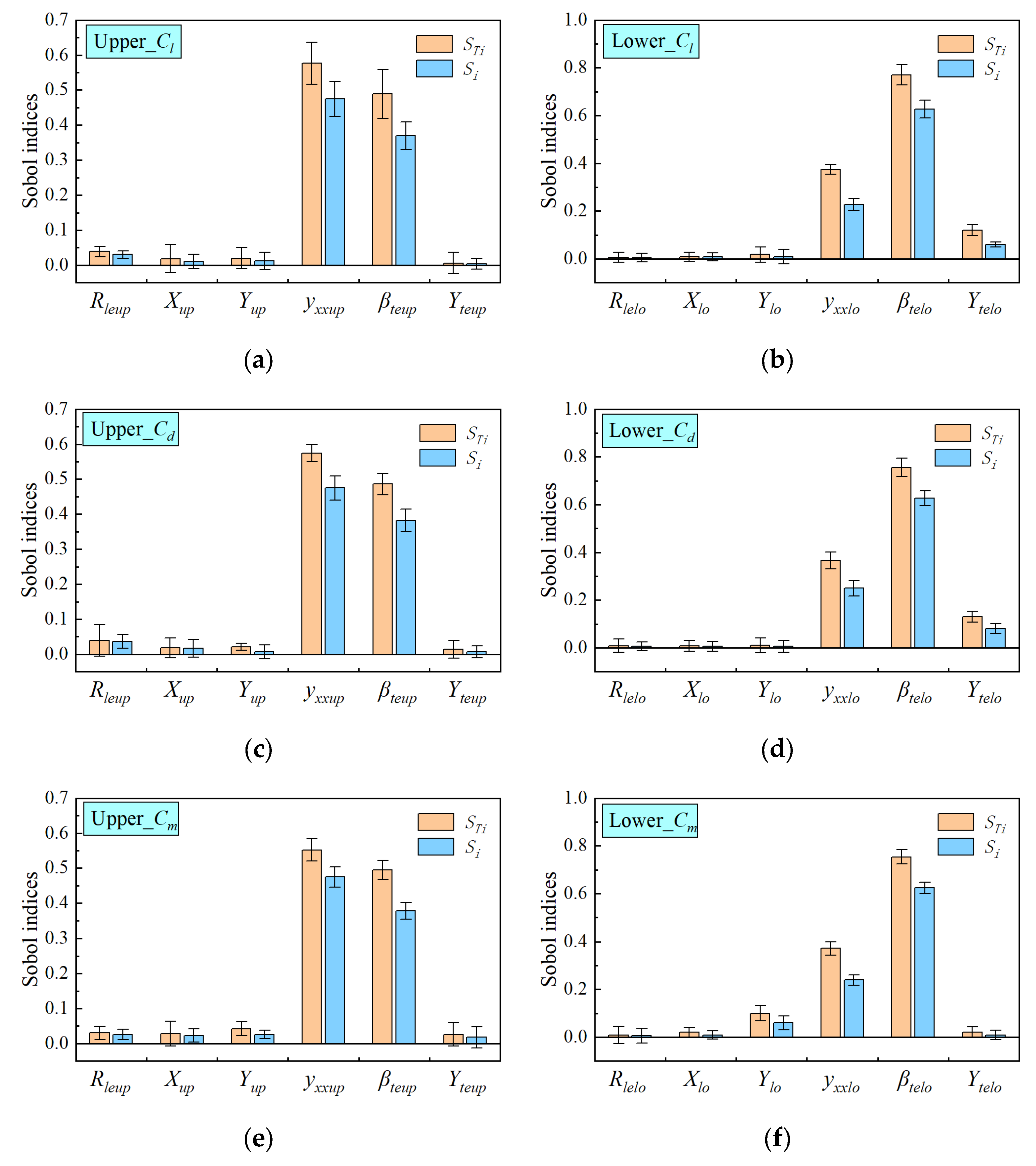
• A global sensitivity analysis framework based on Sobol′s indices is established to quantify the individual and interactive effects of airfoil geometric parameters on dynamic stall characteristics.

The remainder of this paper is organized as follows: Section 2 introduces the concept of Darrieus-type pitching motion (DPM) and its aerodynamic implications for VAWTs. Section 3 outlines the methodology of global sensitivity analysis, including the Sobol method and the construction of the RBFNN-based surrogate model. Section 4 describes the numerical setup and verification process, including the reference case, computational domain, and grid independence analysis. Section 5 presents the results and discussion, focusing on the dynamic stall characteristics under DPM, the performance of the surrogate model, and the sensitivity analysis outcomes. Section 6 summarizes the main conclusions of the study, and Section 7 provides suggestions for future work.

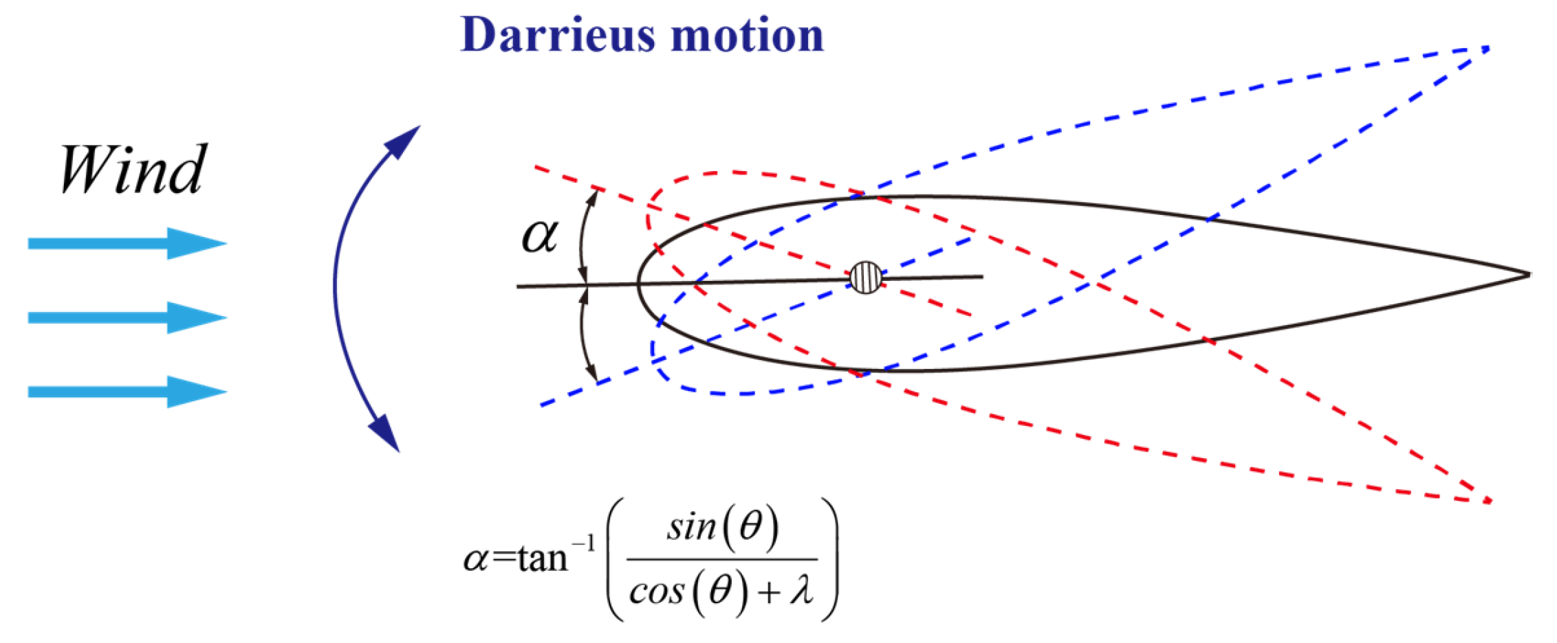
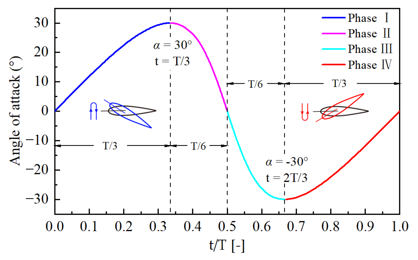
2. Darrieus-Type Pitching Motion (DPM)

When the VAWT is rotating, the velocity triangles of the blade cross-section at different azimuth angles are shown in Figure 2, where V is the incoming wind speed, U is the relative velocity (wind turbine rotation speed), W is the absolute velocity (vector sum of the velocities U and V), θ is the blade azimuth angle, and α is the AoA.

The α of the blade changes continuously with the azimuthal position, and this motion is usually defined as Darrieus-type pitching motion (DPM). The α can be expressed in terms of the tip speed ratio (TSR or λ) and azimuth angle (θ) [9]:

$$\alpha {=\tan }^{-1}\left({\displaystyle \frac{sin\left(\theta \right)}{cos\left(\theta \right)+\lambda }}\right)$$

(1)

The variation curves of α with azimuth for different TSRs are given in Figure 3. It can be seen that the α varies drastically at low TSR. The blade experiences dynamic stall due to the continuous variation of its α and most of the α being large, which has a substantial effect on the aerodynamic performance.

The angular velocity (${\alpha }^{\prime }$) of the VAWT blade DPM is obtained by deriving the time, as shown in Equation (2), where t is the physical time.

$${\alpha }^{\prime }={\displaystyle \frac{\omega \left(\lambda cos\left(\omega \mathrm{t}\right)+1\right)}{{\lambda }^2+2\lambda cos\left(\omega \mathrm{t}\right)+1}}$$

(2)

Figure 4 shows the normalized angle of attack and angular velocity of the blade for different tip speed ratios for one pitching cycle. And it is compared with the sin curve. In Figure 4a, the curve of normalized α does not have a symmetry axis of t/T = 0.25 at 0 < t/T < 0.5 compared to the sin curve. And as the TSR decreases, the position of the maximum angle of attack gets closer to t/T = 0.5. In Figure 4b, the angular velocity of the sinusoidal pitching motion has a gentle slope. However, the angular velocity of the DPM has a sharp slope at t/T = 0.5, which indicates a more drastic change in the angle of attack. This change becomes more noticeable as the TSR decreases.

Dynamic stalls of airfoils have been analyzed by sinusoidal pitching in previous studies. However, in Figure 4, the DPM shows a great difference from the sinusoidal pitch, especially the angular velocity, which is an important factor affecting the development of dynamic stall. Therefore, a comprehensive investigation of DPM is necessary.

3. Methodology for Sensitivity Analysis

This section presents the sensitivity analysis methodology. First, Section 3.1 outlines the theoretical foundations of the Sobol sensitivity analysis method. Due to the Sobol method relying on Monte Carlo sampling and requiring tens of thousands of samples, using high-fidelity CFD models for each evaluation would incur prohibitively high computational costs. To address this, a surrogate model is developed to efficiently approximate the mapping between blade geometric parameters and aerodynamic forces. Section 3.2 details the construction process of the surrogate model based on the radial basis function neural network (RBFNN). Finally, Section 3.3 introduces the complete framework for performing sensitivity analysis using the surrogate model.

3.1. Sobol Sensitivity Analysis Method

The Sobol method is founded on the principle of variance decomposition [35]. It treats the model output as a function of multiple input variables and decomposes the output variance into the contributions attributable to each individual input and their interactions. This approach allows for the quantitative evaluation of how much each input variable (or combination of variables) contributes to the overall variance in the model output, thereby assessing their relative sensitivities [36]. The Sobol sensitivity analysis includes first-order sensitivity indices and total sensitivity indices.

Suppose there is a model with the mathematical expression $Y=f\left(X\right)$, where Y is the model output, X is the vector that consists of n input variables, and each input variable is independent. The model output can be decomposed as [37,38]:

$$\begin{array}{ll}f\left(X\right)& =f_0+{\displaystyle \sum _{i=1}^n{f}_i\left(x_i\right)+{\displaystyle \sum _{1\le i\le j\le n}^n{f}_{ij}\left(x_i,x_j\right)}}+\dots \\ & +f_{12\dots k}\left(x_1,x_2,\dots ,x_n\right)\end{array}$$

(3)

where $f_0$ is the mean value of $f\left(\mathit{X}\right)$, $f_i$ is a first-order function of the input variables, $f_{ij}$ is a second-order function, and so on. All terms of the model response are orthogonal so that there is ${\displaystyle \int f\left(x_i\right)}f\left(x_j\right)d{x}_{i}d{x}_j=0$. Therefore, these decomposition terms can be obtained by calculating the conditional expectation of $Y$. The expression is as follows [35]:

$$f_0=E\left(Y\right)$$

(4)

$$f_i=E\left(Y\left|x_i\right.\right)-E\left(Y\right)$$

(5)

$$f_{ij}=E\left(Y\left|x_i,x_j\right.\right)-f_i-f_j-E\left(Y\right)$$

(6)

The conditional expectation $E\left(Y\left|x_i\right.\right)$ is obtained by calculating the average value of $x_i$ under condition $Y\left|x_i\right.$ in the domain of definition. The larger the $E\left(Y\left|x_i\right.\right)$ corresponding to $x_i$, the higher the impact of the input variable $x_i$ on the output. Hence, the magnitude of sensitivity can be quantified using variance. The total model variance $V\left(Y\right)$ can be written as:

$$V\left(Y\right)={\displaystyle \sum _i^n{V}_i+{\displaystyle \sum _i^n{\displaystyle \sum _{i<j}^n{V}_{ij}+\dots +V_{12\dots n}}}}$$

(7)

where $V_i$ is a short form of $V\left[E\left(Y\left|x_i\right.\right)\right]$. The $V_{ij}$ is the covariance of variables $V_i$ and $V_j$, indicating the contribution of the interaction from the two variables. $V_{12\dots n}$ represents the contribution of all variables interacting together to the output variance.

The Sobol index of each order can be obtained by dividing Equation (7) by $V\left(Y\right)$ as follows:

$$1={\displaystyle \sum _i^n{S}_i+{\displaystyle \sum _i^n{\displaystyle \sum _{i<j}^n{S}_{ij}+\dots +S_{12\dots n}}}}$$

(8)

where the first-order sensitivity $S_i$ and the total index $S_{T_i}$ are defined as [39]:

$$S_i={\displaystyle \frac{V_i}{V\left(Y\right)}}$$

(9)

$$S_{T_i}=1-{\displaystyle \frac{V\left[E\left(Y\left|x_{~i}\right.\right)\right]}{V\left(Y\right)}}$$

(10)

where $x_{~i}$ contains all variables except $x_i$. $V\left[E\left(Y\left|x_{~i}\right.\right)\right]$ is the contribution of all remaining input variables to the output variance when $x_i$ is fixed. Thus, $S_{T_i}$ represent the total contribution of input variable to the output variance both alone and when interacting with other variables.

In order to calculate Sobol’s indices, the steps of random sampling based on Monte Carlo simulation are as follows:

(1)

Generate Monte Carlo samples, which typically requires two sets of input matrices A and B of size (N, n), where n is the number of design variables, and N is the number of samples used for the sensitivity analysis.

(2)

Construct the mixed matrices A⁽ⁱ⁾ and B⁽ⁱ⁾. Replace the i-th column of matrix B with the i-th column of A and keep the rest of the columns to form A⁽ⁱ⁾. Conversely, replace the i-th column of A with the i-th column of B to get B⁽ⁱ⁾.

(3)

Obtain column vectors (Y_A, Y_B, $Y_{A^{\left(i\right)}}$, and $Y_{B^{\left(i\right)}}$) of size (N, 1) by evaluating the model from A, B, A⁽ⁱ⁾, and B⁽ⁱ⁾, which defined as:

$$Y_A=f(A), Y_B=f(B), Y_{A^{\left(i\right)}}=f(A^{\left(i\right)}), Y_{B^{\left(i\right)}}=f(B^{\left(i\right)})$$

(11)

(4)

Calculate the first-order index and the total index for the i-th input variable using the following equations:

$$S_i={\displaystyle \frac{\frac{1}{N}{\displaystyle {\sum }_{j=1}^N{Y}_A^{(j)}\cdot (Y_{A^{(i)}}^{(j)}-Y_B^{(j)})}}{V(Y)}}$$

(12)

$$S_{Ti}=1-{\displaystyle \frac{\frac{1}{N}{\displaystyle {\sum }_{j=1}^N{Y}_B^{(j)}\cdot (Y_{B^{(i)}}^{(j)}-Y_A^{(j)})}}{V(Y)}}$$

(13)

The accuracy of the Sobol sensitivity analysis is highly dependent on the sample size N. As the N increases, the results become more accurate.

3.2. Surrogate Model Method

During sensitivity analysis, thousands of input samples are typically required to evaluate the variance between input parameters and model outputs. However, conducting high-fidelity CFD simulations for such large datasets is computationally expensive and time consuming [40,41]. Therefore, in this work, a radial basis function neural network (RBFNN) surrogate model is developed to approximate the mapping relationship between blade geometric parameters and aerodynamic characteristics associated with dynamic stall. The construction of the RBFNN surrogate model includes the following key steps: airfoil parameterization, Latin Hypercube Sampling for generating training data, surrogate model training, and model accuracy validation.

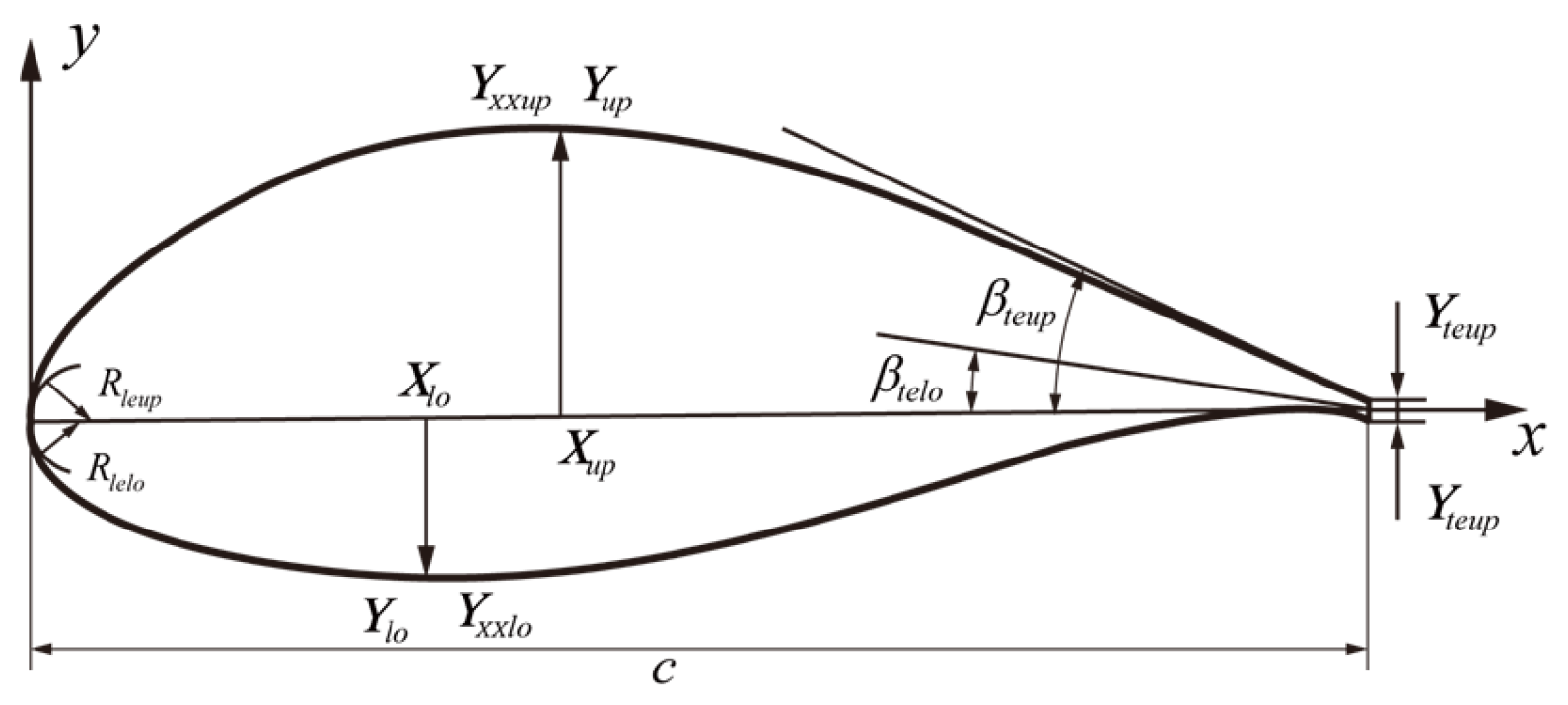
3.2.1. PARSEC Parameterization

The common airfoil parameterization methods are the characteristic parameter method (PARSEC), the type function perturbation method (Hicks–Hence type function), the control point method (Bezier and B-Spline curves, etc.), and the orthogonal basis function (CST method). Unlike other parameterization methods, the PARSEC method provides a group of parameters to directly describe the airfoil’s geometrical shape, with the advantage of a well-defined geometrical meaning [42,43]. Figure 5 shows the airfoil geometry shape using 12 PARSEC parameters.

Table 1. The description of PARSEC parameters.

PARSEC Parameters	Description
$R_{leup}$ ($R_{lelo}$)	Upper (low) surface leading-edge radius
$X_{up}$ ($X_{lo}$)	Upper (low) surface maximum thickness position
$Y_{up}$ ($Y_{lo}$)	Upper (low) surface maximum thickness
$Y_{xxup}$ ($Y_{xxlo}$)	Upper (low) surface curvature at the position of maximum thickness
$Y_{teup}$ ($Y_{telo}$)	Upper (low) surface trailing-edge thickness
${\beta }_{teup}$ (${\beta }_{telo}$)	Upper (low) surface deflection angle of the trailing edge

shows the description of the PARSEC parameters.

The symmetrical airfoil NACA0018, commonly used for vertical-axis wind turbines, has 12 PARSEC geometric parameters on the upper and lower surfaces, as shown in

Table 2. The PARSEC geometry parameters of NACA0018.

Upper	Value	Lower	Value
$R_{leup}$	0.1412	$R_{lelo}$	0.1412
$X_{up}$	0.2974	$X_{lo}$	0.2974
$Y_{up}$	0.0900	$Y_{lo}$	0.0900
$Y_{xxup}$	0.6719	$Y_{xxlo}$	−0.6719
$Y_{teup}$	0.0019	$Y_{telo}$	−0.0019
${\beta }_{teup}$	11.7751	${\beta }_{telo}$	−11.7751

.

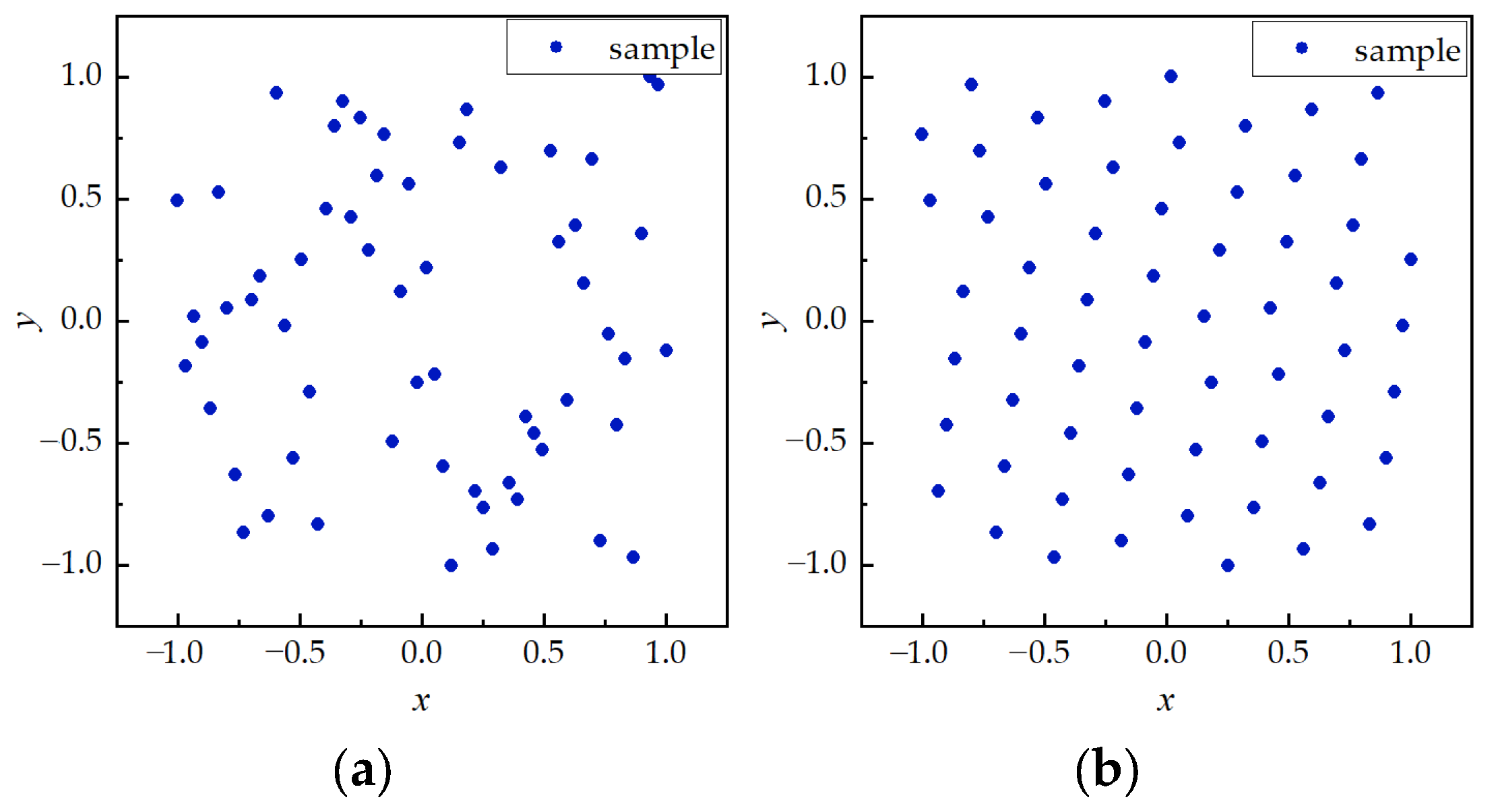
3.2.2. Optimized Latin Hypercube Sampling (OLHS)

Latin Hypercube Sampling (LHS) is a random sampling method based on Monte Carlo simulation [44]. In the multidimensional parameter space, there is an over-concentration of sample points. The spatial distribution among the sampling points is optimized according to the maximum–minimum distance criterion to conduct optimized LHS (OLHS) to improve the uniformity of the sample points [45].

Assume n is the number of samples and d is the spatial dimension. Use the LHS to generate an n × d matrix, where the column vectors are randomly ordered as {1, 2, …, n} and normalized to the interval [0, 1), as follows:

$$L_{ij}={\displaystyle \frac{1}{n}}\left({\pi }_{ij}-U_{ij}\right)$$

(14)

where ${\pi }_{ij}$ is a random arrangement of {1, 2, …, n}, and $U_{ij}$ is a uniform random number in the interval [0, 1).

If there are two sample points $z_{ik}$ and $z_{jk}$, the Euclidean distance is calculated as follows:

$$d_{ij}=\sqrt{{\displaystyle {\sum }_{k=1}^d{\left(z_{ik}-z_{jk}\right)}^2}}$$

(15)

The objective of maximizing the minimum distance between each sample point is achieved using nonlinear least squares method. Taking the two-dimensional (2D) space as an example, a comparison of sampling using LHS and OLHS is shown in Figure 6. Although the LHS method can complete the sampling in the entire space, the local spatial homogeneity is not good, and the distribution of the sample points obtained by the OLHS method is more homogeneous and can capture most of the features of the space.

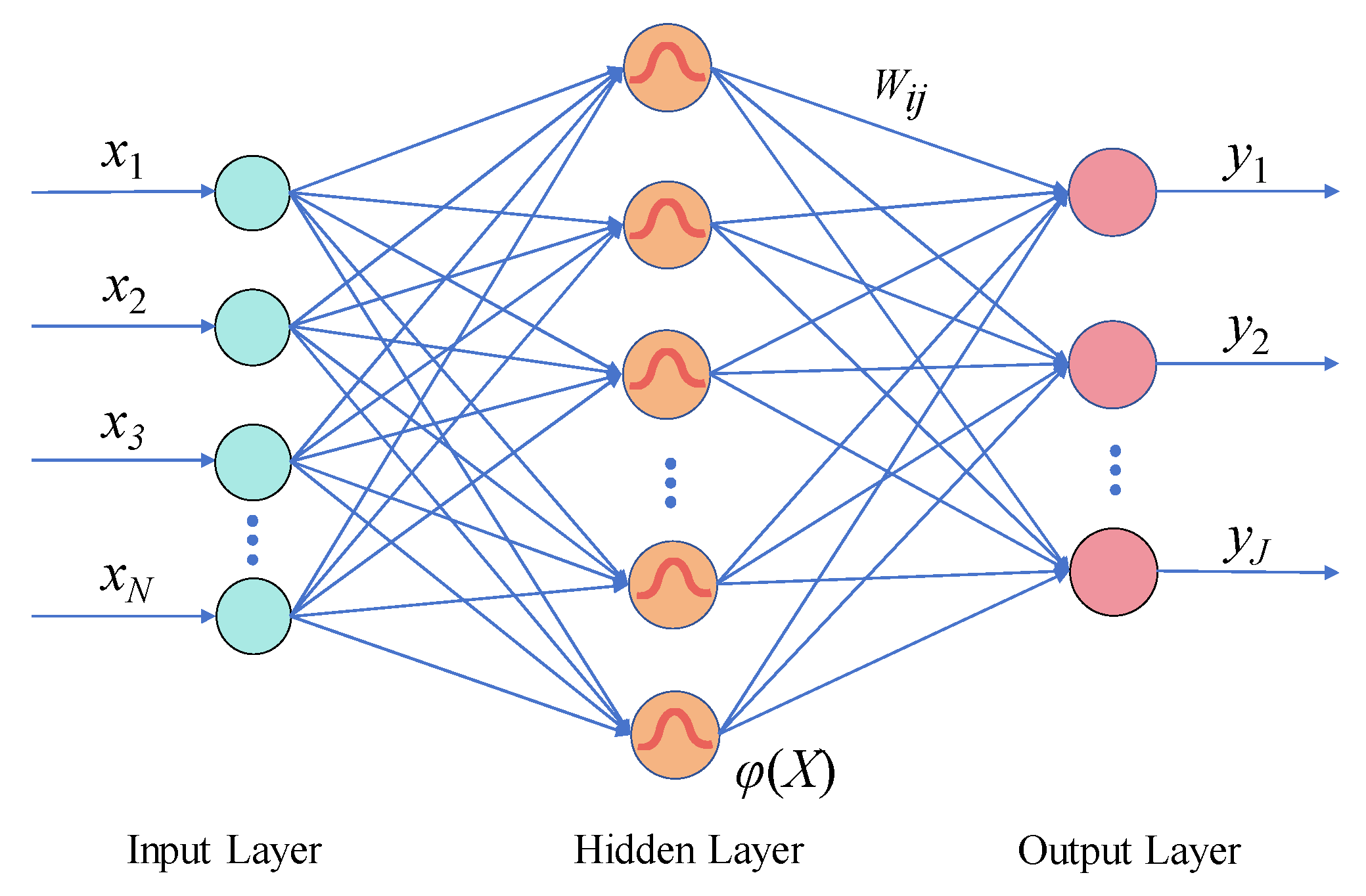
3.2.3. Radial Basis Function Neural Network (RBFNN)

The RBFNN is a three-layer forward network with strong mapping capabilities that fits well to arbitrary systems of both deterministic and stochastic response functions [46,47]. It is commonly used for tasks such as function approximation, classification, and prediction. It consists of a three-layer network structure with an input layer, a hidden layer, and an output layer, as shown in Figure 7.

The main feature of the RBFNN is the use of radial basis functions as implicit layer activation functions. Commonly used is the Gaussian function [48,49]:

$${\phi }_j\left(X\right)=\exp \left(-{\displaystyle \frac{\Vert x_i-{c_i\Vert }^2}{2{\sigma }_j^2}}\right)$$

(16)

where X is the input vector, $X=\left(x_1,x_2,x_i,\dots x_N\right)$, and ${\phi }_j\left(x\right)$ is the j-th radial basis function. $c_j$ is the j-th centroid, and each radial basis function corresponds to a centroid; ${\sigma }_j$ is the width parameter of the j-th unit.

Firstly, the hidden layer maps the low-dimensional data of the input layer to a higher-dimensional space by using the Gaussian activation function to express more information. Secondly, the results of the hidden layer are linearly combined with the corresponding weight coefficients. Finally, the model output is obtained through computation. The process of the RBFNN can be expressed as [49]:

$$Y\left(X\right)={\displaystyle \sum _{i=1}^M{\omega }_{ij}{\phi }_j\left(x_i\right)}$$

(17)

where Y is the output vector, $Y=\left(y_1,y_2,y_j,\dots y_J\right)$, $y_j\left(x\right)$ is the output of the j-th unit, M is the number of neurons in the hidden layer, and ${\omega }_{ij}$ is the weight coefficients for the i-th unit in the hidden layer and the j-th unit in the output layer.

3.2.4. Validation of Surrogate Model

The accuracy of the surrogate model is especially critical for sensitivity analysis. In order to validate the accuracy of the established RBFNN model, this paper evaluates the model using the Mean Squared Error (MSE), Root Mean Squared Error (RMSE), and Coefficient of Determination (R-squared, R²) [50].

$$\mathrm{MSE}={\displaystyle \frac{1}{n}}{\displaystyle \sum _{i=1}^n\left(y_i-{\widehat{y}}_i\right)}$$

(18)

$$\mathrm{RMSE}=\sqrt{{\displaystyle \frac{1}{n}}{\displaystyle \sum _{i=1}^n\left(y_i-{\widehat{y}}_i\right)}}$$

(19)

$$R^2=1-{\displaystyle \frac{{\displaystyle {\sum }_{i=1}^n\left(y_i-{\widehat{y}}_i\right)}}{{\displaystyle {\sum }_{i=1}^n\left(y_i-{\overline{y}}_i\right)}}}$$

(20)

Here, $y$ is the simulated value by CFD, $\widehat{y}$ is the value predicted by the RBFNN, and $\overline{y}$ is the mean of the simulated value.

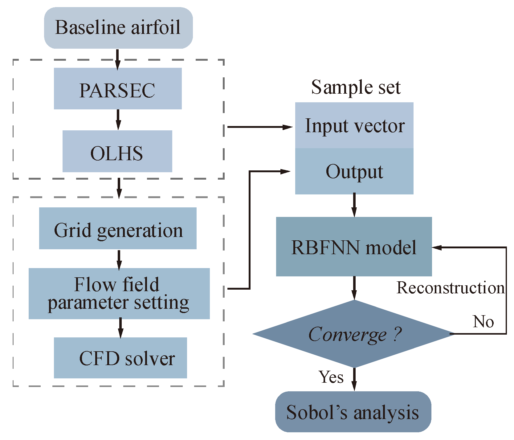
3.3. Sensitivity Analysis Process

The sensitivity analysis process involves a lot of repetitive work realized through batch commands, including grid generation, case submission, and data processing. These different steps (as shown in Figure 8) are realized using MATLAB 2024R2 scripts by calling different modules. The steps are as follows:

(1)

Using the PARSEC parameterization method, we obtain the 12 geometric parameters for the upper and lower surfaces of the airfoil NACA0018.

(2)

The OLHS method is applied to obtain 200 initial samples in the design space as the input vector x. The aerodynamic coefficients are solved using the CFD method as the output response y.

(3)

The RBFNN model is constructed using the dataset (x, y). There are 180 samples in the training set and 20 in the test set. The accuracy of the model is verified by the MSE, RMSE, and R². If the convergence error is not satisfied, we retrain the model by adjusting the neural network parameters.

The Monte Carlo simulation is used to prepare samples and obtain a fast response based on the trained RBFNN model. Next, we use Sobol’s method to calculate the first-order sensitivity indices and higher-order indices for each geometric parameter.

4. Numerical Modeling and Verification

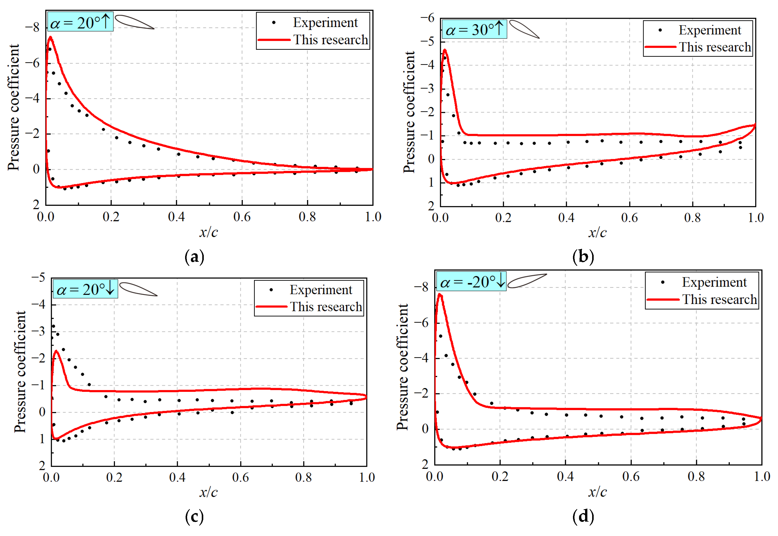
This section describes the flow parameter settings in the CFD model. First, an experimental study of DPM is introduced. Next, the computational domain grid and boundary conditions for 3D numerical simulations are presented. Then, the flow solver and its settings are described. Finally, the research results for the validation of grid and time independence are given.

4.1. Reference Case

For the DPM research, Wickens [51] conducted an experimental study of the NACA0018 airfoil in a 2 × 3 m wind tunnel at the Low-Speed Aerodynamics Laboratory of the National Research Council in Canada. The blades are mounted vertically in the wind tunnel. The DPM around the airfoil’s aerodynamic center is shown schematically in Figure 9. The red and blue dashed lines indicate positive and negative angles of attack, respectively. The rotating shaft located at the aerodynamic center is combined with bearings at the top and bottom of the wind tunnel. The bearings are also connected to the lever mechanism of the hydraulic actuator. Finally, the control system is utilized to realize the pitching motion of the airfoil at different tip speed ratios.

In the wind tunnel experiments, the blade experiences an incoming wind speed of 45.72 m/s and a Reynolds number of 1.91 × 10⁶. The 45.72 m/s flow velocity applied to the single blade represents the resultant velocity incorporating rotational effects. Fundamentally, the Darrieus-type pitching motion (DPM) replicates the VAWT blade’s kinematic behavior during VAWT rotation. The airfoil chord length is 0.61 m. Several pressure sensors are installed on the airfoil surface to acquire pressure data at 45 points. The oscillation frequency is set to 0.55 Hz. The sampling frequency is 250 Hz to collect pressure data during the oscillation cycle. This process records the detailed transient pressure data on the airfoil. Subsequently, the normal and tangential force coefficients of the airfoil are calculated from these pressures.

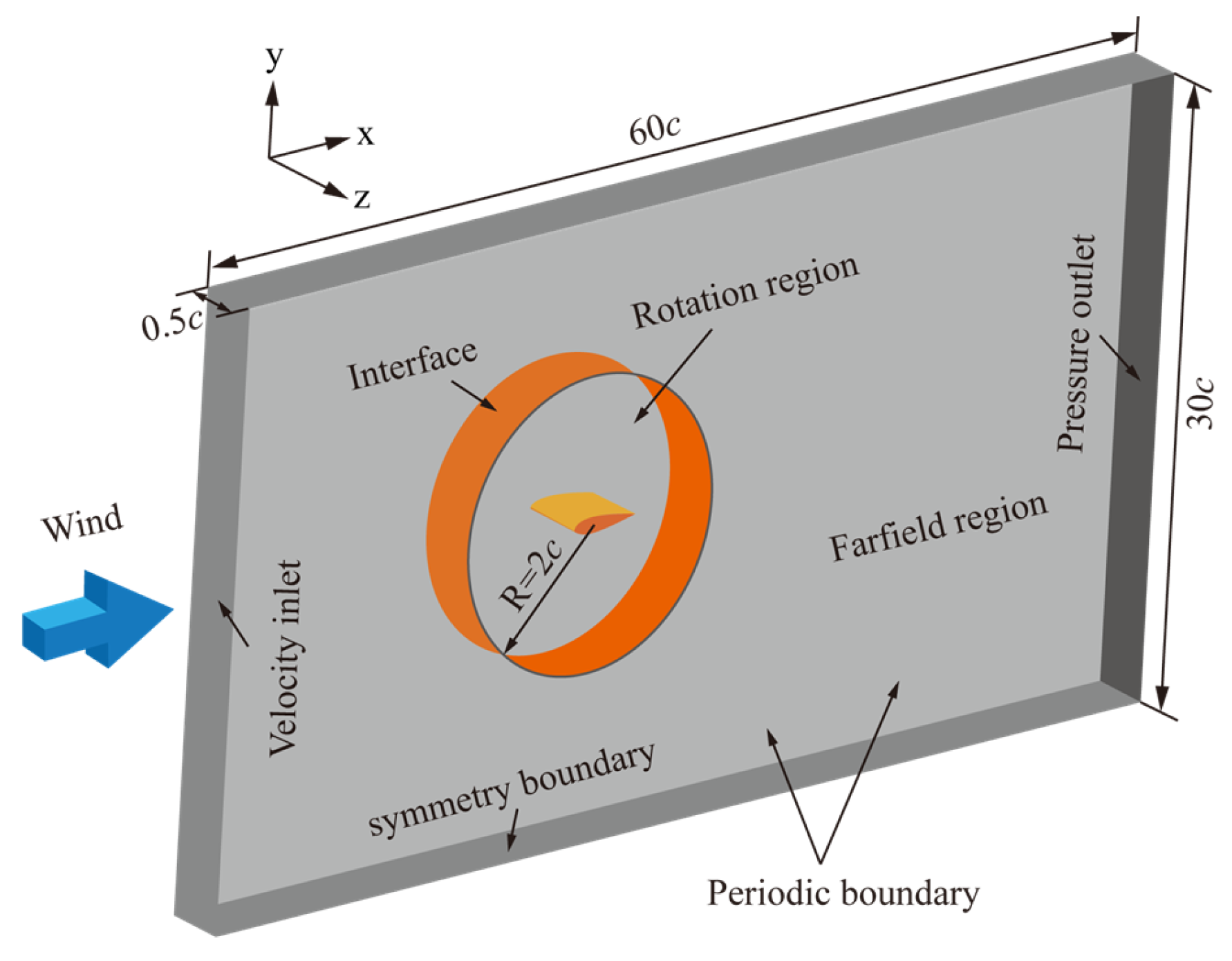
4.2. Computational Domain and Grid

The size and boundary conditions of the quasi-3D computational domain are shown in Figure 10. In order to eliminate the influence of boundary conditions on the accuracy of numerical simulation, the size of the computational domain is set to 30 × 60c. This distance is sufficient to avoid the boundary influence on the airfoil flow state. The thickness of the blade spreading direction is 0.5c.

The computational domain is divided into the outer domain and the rotational domain. The aerodynamic center of the blade coincides with the center of the rotational domain of radius 2c. The sliding mesh technique is used to realize the pitch oscillation motion of the rotating domain with respect to the stationary domain. And a user-defined function (UDF) program is written within the solver to control the rotational domain motion according to the law of Equation (2). The left and right sides of the computational domain are set as velocity inlet and pressure outlet, respectively. The top and bottom sides are symmetric boundaries, and the front and back sides are periodic boundaries. The airfoil surface is set as a no-slip wall.

The primary task in numerical simulation is gridding, and a well-quality grid can improve computational accuracy and convergence speed. In this work, the hexagonal grid is considered to be applied to the computational domain to improve the grid quality. The grid of the computational domain and the local details of the blade are shown in Figure 11. The grid near the blade surface is refined to better capture the complex flow generated within the boundary layer during dynamic stall. The height of the first layer of the boundary layer is 0.01 mm to ensure that y+ is approximately equal to 1.

4.3. Independence Verification

The grid resolution and the time step are two important factors in determining the dynamic stall characteristics and the computational accuracy. The objective is to obtain a balance between simulation cost and accuracy. Therefore, it is necessary to investigate the grid and time independence to accurately obtain the aerodynamic results during the dynamic stall pitching motion.

The unsteady Reynolds-averaged Navier–Stokes (URANS) equations are solved using STAR CCM+ 2310 software. The turbulence model is SST k-ω. The flow parameters are chosen in agreement with Wickens et al. [49]. The internal iterations for each time step are 30, and the convergence criterion is set to 10⁻⁶. According to the literature [52], the boundary layer flow state of the VAWT blade can be better captured under unsteady conditions by using the SST k-ω turbulence model. The pressure–velocity coupling is based on the SIMPLE algorithm. The second-order upwind scheme is used for the control equations, and the second-order implicit scheme is used for the time discretization.

The coefficient of lift (C_l) and coefficient of drag (C_d) are important aerodynamic parameters for evaluating the blade performance, and their mathematical expressions are as follows [53].

$$C_{l,d}={\displaystyle \frac{F_l,F_d}{0.5\rho V_{\infty }^{2}S}}$$

(21)

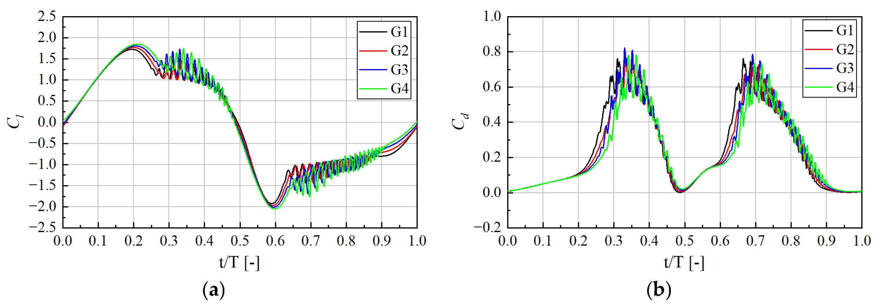
4.3.1. Grid Independence Verification

Four different sizes of grid resolution are set to study grid independence, as shown in

Table 3. Detailed information of grid parameters.

Parameters	Number of Grids	Height of First Layer/(mm)	Surface Grid Growth Rate	Volume Grid Growth Rate
G1	145 × 104	0.04	1.10	1.15
G2	191 × 104	0.02	1.05	1.10
G3	227 × 104	0.01	1.02	1.05
G4	255 × 104	0.01	1.02	1.02

. The computational domain grid is gradually refined with the decrease in size.

Figure 12 shows the aerodynamic forces of DPM for one pitching cycle at λ = 2. To ensure numerical stability, the aerodynamic results of the 5th cycle are selected for analysis. It can be clearly seen that two dynamic stalls occurred in one cycle and the second stall lasted longer. In the aerodynamic stabilization phase, the increase in the number of grids has less effect on the aerodynamic forces because the fluid is attached to the airfoil surface. In the phase where the dynamic stall occurred, the difference in the number of grids affected the aerodynamic results due to the flow separation. This indicates that a sufficiently fine grid is needed to capture the boundary layer flow. In Figure 12, the difference of C_d in the stall phase is larger for the four grid numbers compared to C_l. There is a significant deviation between G1 and G2 during the stall phase. The aerodynamic changes are smaller when the grid number grows to G3 and G4. However, the simulation time increases significantly due to the more refined grid of G4. Therefore, the grid number of G3 is chosen for further numerical simulations.

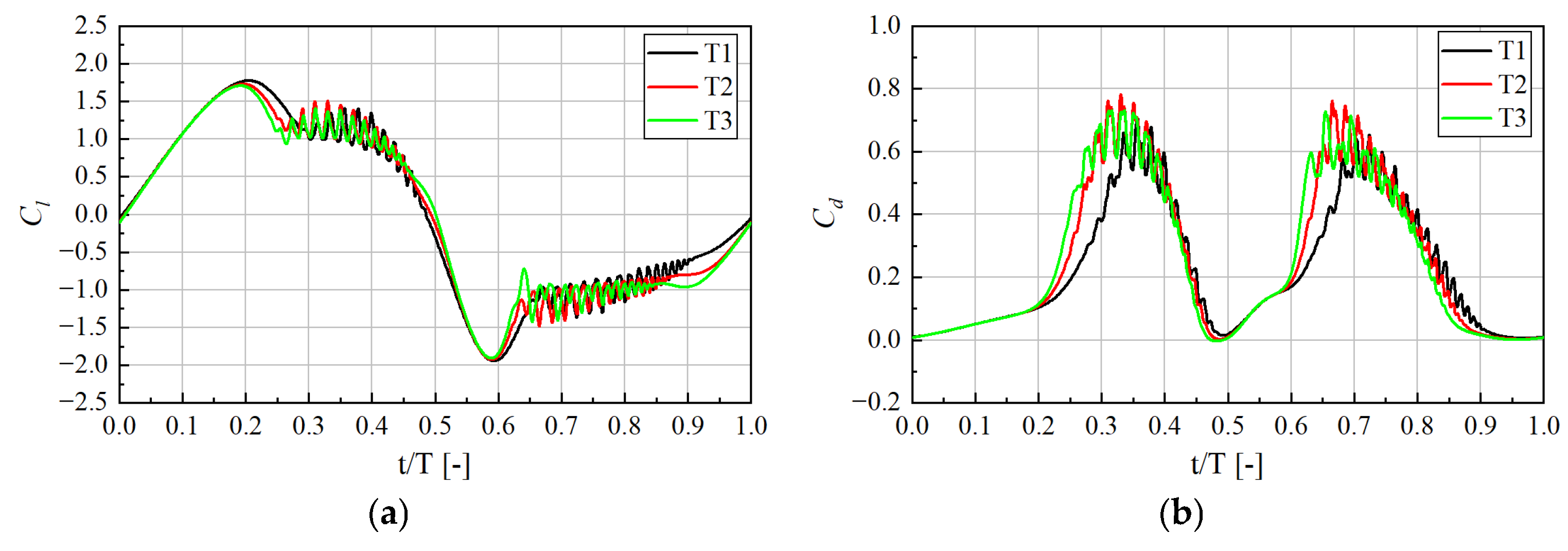
4.3.2. Time Independence Verification

For the single blade simulation, the angle of attack experienced in one pitch cycle actually represents one round turn of the VAWT’s rotor. Therefore, the time step for DPM should be related to the rotation angle of the VAWT. The time steps corresponding to 0.5°, 0.25°, and 0.125° of VAWT rotation are selected for simulating single-blade pitching to analyze the time sensitivity. The detailed parameters of the time step are shown in

Table 4. Parameters of time step.

Parameters	Time Steps/(10−4)	VAWT Rotation Angle at Each Time Step	Wall Clock/Hour
T1	25.25	0.5°	5.51
T2	12.62	0.25°	11.25
T3	6.31	0.125°	22.05

.

The time step sensitivity of the DPM at λ = 2 is investigated. Figure 13 shows the variation in the aerodynamic coefficients for one pitching cycle. As shown, a smaller time step is required to refine the simulation due to the highly unsteady flow phenomena during the stall phase. When the time step is changed from T1 to T2, it is observed that the angle of attack decreases faster after t/T = 0.2, which implies that an earlier flow separation occurs. This indicates that T1 is not able to accurately simulate the critical state of aerodynamic deterioration. There is a little difference between T2 and T3 during the aerodynamic oscillation phase, and the predictions of the flow separation point are very similar. In addition, the simulation time for T3 is almost double that of T2. Therefore, in order to balance the computational accuracy and time cost, the time step of T2 is selected for aerodynamic data acquisition.

5. Results and Discussion

The pressure coefficients can reflect the flow details on the blade surface. The results of the pressure coefficients for 3D simulation and the experimental values in the wind tunnel are shown in Figure 14, where ↑ represents the upstroke phase of the blade, and ↓ is the downstroke phase. At α = 20° ↑, the pressure coefficients from the numerical simulation closely match the experimental values because no flow separation occurs on the blade. As the α increases, at α = 30° ↑, the simulation accurately fits the pressure distribution on the upper surface. In the downstroke phase with α decreasing, the leading-edge pressure coefficient predicted by the simulation only exists at the upper surface. It can be observed that when α = 20° ↓ and −20° ↓, the numerical simulation is already sufficient of capturing the flow characteristics on the blade surface. The 3D simulation has the advantage of capturing the flow in the spanwise direction of the blade and, therefore, predicts the pressure coefficients well. For the 200 initial samples in the sensitivity analysis module, only the blade shape is changed, and no add-on devices are created. Therefore, the high-precision CFD model parameters established in this section also support the subsequent flow field calculations.

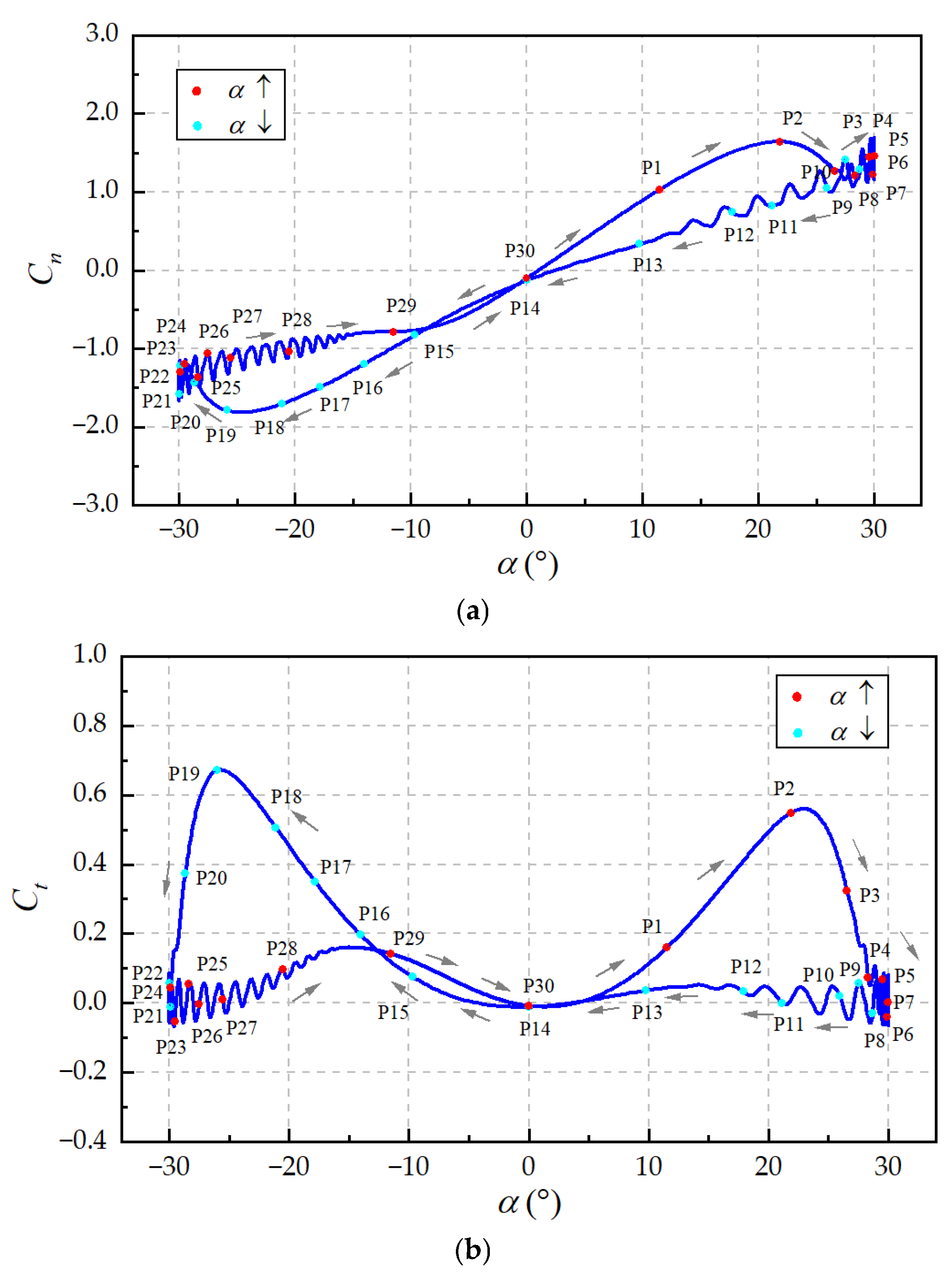
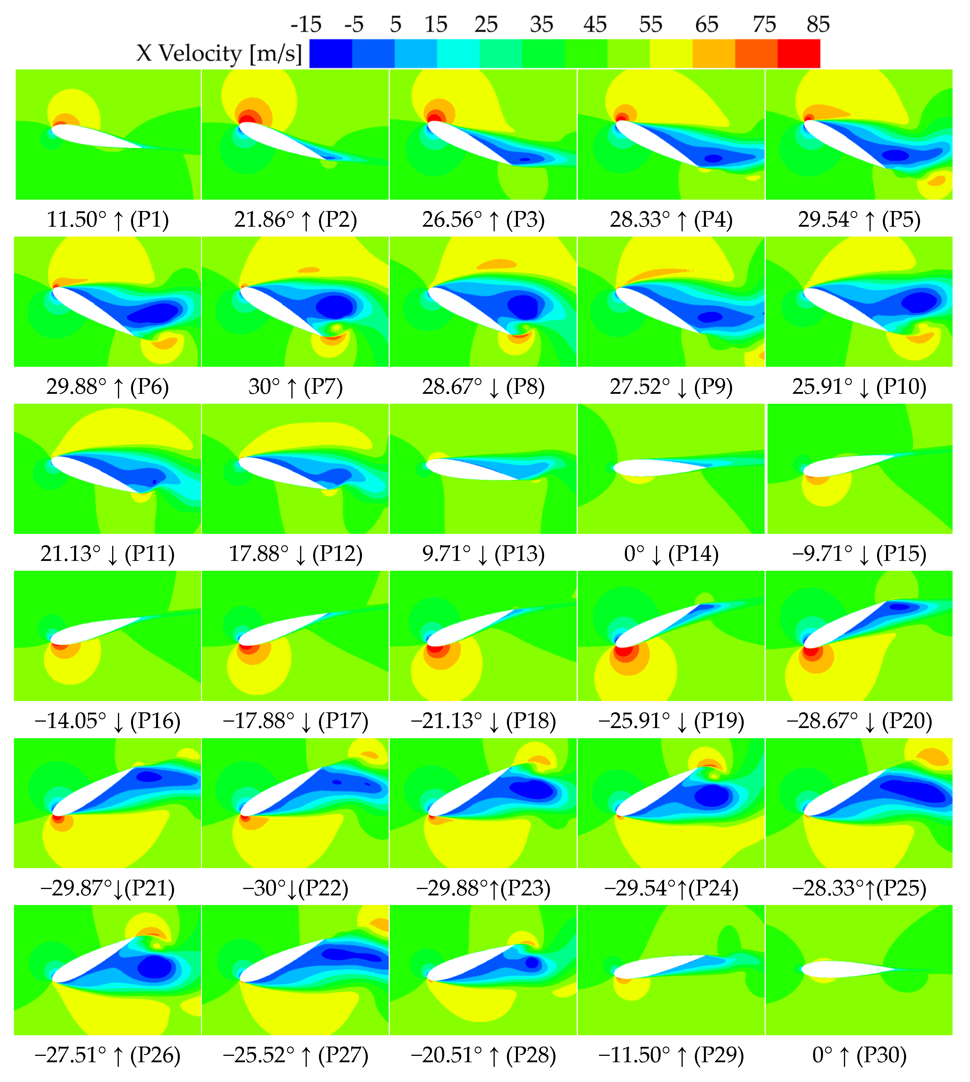
5.1. Flow Field Structure of DPM

Taking a tip speed ratio of λ = 2 as an example, the variation of the α for DPM can be divided into four distinct phases, as shown in Figure 15, each marked by different colors. When the blade rotates clockwise, α is defined as positive, with the positive and negative signs indicating only the direction of motion. Both Phase I and Phase III involve an increase in α from 0° to 30°; however, the duration of Phase III is only half that of Phase I, lasting just T/6. Similarly, α decreases from 30° to 0° during Phases II and IV, but Phase II also lasts only T/6. Overall, in the interval [0-T/2], α experiences a gradual increase followed by a rapid decrease, while in the interval [T/2-T], the opposite occurs. This results in differing pitch angular velocities across the four phases, indicating that the pitching motion is not symmetric. It is worthwhile to study the effect of sudden changes in angular velocity on the flow.

The normal force (F_n) and tangential force (F_t) are important parameters to characterize the aerodynamic performance of VAWT blades. They are critical for the aerodynamic design of offshore VAWTs. The equation for the normal force coefficient (C_n) and tangential force coefficient (C_t) in dimensionless form is as follows:

$$C_{n,t}={\displaystyle \frac{F_n,F_t}{0.5\rho V_{\infty }^{2}S}}$$

(22)

Figure 16 shows the simulated results of the DPM for Cn and Ct over one cycle for λ = 2. The P1–P30 are 30 successively marked points (different colors representing α in an increasing or decreasing state) corresponding to Figure 17, which describes the instantaneous velocity contours of the unsteady flow structure during one cycle. The evolution of flow physics is determined by observing the blade dynamic stall to fully understand the DPM.

In Phase I (P1–P7), the fluid is completely attached to the airfoil surface when α < 11.5° ↑. As α increases, the trailing edge forms a reverse flow due to the reverse velocity gradient (the blue low-velocity flow region at α = 21.86° ↑). At this point, although flow separation occurs, it has less effect on the high-velocity region of the trailing edge. Nevertheless, also from α = 21.86° ↑, the aerodynamic forces begin to decrease, as observed from the C_n curve in Figure 16a. At α = 26.56° ↑, the separation flow extends to the leading edge. At α = 29.54° ↑, the high-velocity region at the leading edge of the upper surface starts to diffuse due to the excessively large α, and the leading-edge velocity completely diffuses when the blade reaches α = 30° ↑. The trailing-edge reverse-flow region dominates the flow. The leading-edge stall deteriorates the flow unsteady and leads to severe aerodynamic oscillations (P4–P7 in Figure 16).

During the downstroke of Phase II, the leading-edge high-velocity region is in a stall condition. Although the α is gradually decreasing, the high-velocity region does not recover and remains in an unsteady state (P8–P11 in Figure 16). This is primarily because the blade’s downstroke motion is opposite to the incoming flow direction, preventing α (despite being sufficiently small) from re-establishing high-velocity fluid attachment near the leading edge. The reverse flow at the trailing edge gradually diminishes as α decreases. When α = 0° ↓, the flow velocity at the lower surface is already higher than that at the upper surface due to fluid inertia because the blade pitch angle velocity is not zero (P14 in Figure 16).

Phase I and Phase III are both processes that involve a gradual increase in α from 0 to 30°. However, Phase III has a larger angular velocity because the time of Phase III is only half of that of Phase I. The difference between them is mainly in the high-velocity region of the leading edge where α is larger. Compared to Phase I, when α > −28.67° ↓, Phase III has only slight velocity diffusion even though the leading-edge high-velocity region is also changing. There is still a high aerodynamic force at α = −30° ↓ (P22 in Figure 16, with the leading-edge high-speed region in red in Figure 17). This phenomenon demonstrates that the rapid diffusion of leading-edge velocities is correlated with blade angular velocities. In addition, a larger and more pronounced trailing-edge low-velocity region exists in Phase I (P7 and P22 in Figure 17), indicating that the larger blade pitch angular velocity mitigates the trailing-edge separation flow.

Similarly, disregarding the direction, the α of Phase IV and Phase II decreases gradually from 30° to 0°, and the angular velocity of Phase IV is smaller. It can be observed that the leading-edge high-velocity region gradually diffuses and completely diffuses in a very short time at α = −29.54° ↑. At α = −29.54° ↑–(−20.51° ↑), both leading-edge stall and trailing-edge reverse flow co-exist. Near α= −11.50°↑, the leading-edge velocity begins to recover, and high-velocity fluid is regenerated (P29 in Figure 17). Compared with Phase II, the blade’s leading-edge velocity recovers faster, which indicates that the smaller the pitch angular velocity is, the faster the velocity recovers. In addition, at α = 0° ↑, the slower angular velocity at this time causes the velocities on the upper and lower surfaces to be almost the same, and the phenomenon of higher velocities on one side at α = 0° ↓ is not observed.

Large offshore floating VAWTs are usually operated at a high Reynolds number; therefore, in order to investigate the effect of the Reynolds number on the dynamic stall performance of the blades, the case of Re = 5 × 10⁶ will be compared. Figure 18 shows the effect of increasing the Reynolds number on the normal and tangential force coefficients.

At a high Reynolds number, the unsteady condition of the aerodynamic coefficients is greatly reduced, and the fluctuations are obviously reduced. As seen in Figure 18a, at a larger α, when the Reynolds number increases, the stall α is delayed backward from 21.2° to 26.7°, resulting in an increase in the maximum normal force coefficient. Only slight oscillations exist near 30°, and the aerodynamic fluctuations are small for the rest of the angles of attack. In Figure 18b, the larger Reynolds number causes the C_t to increase in a larger range of α, and the increase in the C_t improves the self-starting performance at low tip speed ratios.

In summary, a higher Reynolds number enhances the aerodynamic efficiency and self-starting capability of the VAWT while also mitigating the adverse effects of unsteady aerodynamic forces associated with blade dynamic stall. Furthermore, the stabilization of aerodynamic coefficients contributes to improved structure performance and reliability of the VAWT system.

As the Reynolds number increases, the aerodynamic coefficients show a large difference at large angles of attack. To further investigate the aerodynamic changes, Figure 19 shows the comparison of pressure coefficients on the blade surface at different Reynolds numbers for larger angles of attack. At α = 20° ↑, α = −20° ↓, there is almost no difference in the pressure coefficient due to the small AoA (e.g., Figure 19a,e); when α = 25° ↑, α = 30° ↑ vs. α = 25° ↓, the leading-edge differential pressure decreases at small Reynolds numbers as the AoA increases, while increasing the Reynolds number makes the leading-edge differential pressure increase significantly (e.g., Figure 19b–d).

At α = −25°↓, it can be observed that the difference in leading-edge differential pressure at different Reynolds numbers is small, the reason being that the leading edge of the blade at Phase III, Re = 1.91 × 10⁶, does not stall, so the difference is not large. At α = −30° ↓, α = −25° ↑, and α = −25° ↑, these angles of attacks are at a low Reynolds number, resulting a drastic leading-edge stall, and the aerodynamic force is significantly reduced; increasing the Reynolds number suppresses the leading-edge stall, so the aerodynamic performance of the blade is effectively increased.

5.2. RBFNN Surrogate Model

The PARSEC method is used to extract 12 geometric parameters for the NACA0018 airfoil. The sampling space is defined by allowing each parameter to vary within ±20% of its baseline value. A total of 200 airfoil samples are generated by OLHS. For each sample, the average lift, drag, and moment coefficients over one pitch cycle are calculated using the CFD method described in Section 4. The resulting input matrix has the dimensions 12 × 200, and the corresponding output matrix is 3 × 200. These 200 sample pairs are used to construct the RBFNN surrogate model, with 180 samples allocated for training and the remaining 20 reserved for testing.

The RBFNN models are constructed for the upper and lower surfaces of the blade, respectively.

Table 5. Prediction accuracy of the RBFNN model.

Evaluation Index	MSE	RMSE	R2
Upper	0.000875	0.0295	0.982
Lower	0.000953	0.0324	0.975

shows the accuracy of the surrogate models calculated by different evaluation indexes. Among them, an R² closer to 1 represents that the model is closer to the original function. The R² of the surrogate model constructed in this work is 0.982 and 0.975 for the upper and lower surfaces, respectively, which is considered to predict the aerodynamic results of the DPM better.

Figure 20 shows the comparison between the predicted results of the RBFNN model and the CFD simulated values. The RBFNN model shows an excellent result in predicting the aerodynamic forces due to its ability to fit and approximate the nonlinear data. In this work, the trend of the predicted values is generally in agreement with the simulated values. There are no points that are very inaccurate, except for deviations in some sample points. From Figure 20a, the RBFNN model predicts the averaged C_d and C_m better than the C_l, especially the C_d. From Figure 20b, it is observed that the predictions of the averaged C_l and C_m are more accurate.

5.3. Sensitivity Analysis

The surrogate model offers a fast and accurate means of evaluating the aerodynamic forces acting on the blade, making it well suited for conducting global sensitivity analysis with respect to geometric parameters. In this study, Sobol indices are computed using Monte Carlo simulation (MCS). The number of samples required for MCS is determined based on the convergence behavior of the Sobol indices, ensuring sufficient accuracy in quantifying the sensitivity of each input parameter. The convergence results for the number of samples required for S_i and S_Ti are shown in Figure 21. It converges when the sample size reaches 10⁵. The MCS is repeated 100 times to calculate the Sobol indices to obtain the average Sobol indices and standard deviations for each geometrical parameter. The reason for the negative sign in the Sobol index is due to numerical computation error when the index is close to zero.

Figure 22 shows the sensitivity analysis results of the averaged aerodynamic coefficients with respect to the geometric parameters. For the blade upper surface, the most important parameters that affect the stall characteristics of the DPM are the curvature at maximum thickness ($y_{xxup}$) and trailing-edge deflection angle (${\beta }_{teup}$). The reason is that the state of fluid attachment during blade pitching is very much related to the surface curvature, which directly leads to the variation in the stall characteristics. In Figure 22a,c, the leading-edge radius ($R_{leup}$) has a higher effect on the averaged C_l and C_d than the maximum thickness position ($X_{up}$) and the maximum thickness ($Y_{up}$). However, in Figure 22e, the effect of the $Y_{up}$ on the averaged C_m is more significant because the variation of the thickness is related to the ability of the blade to resist deformation. The trailing-edge thickness ($Y_{teup}$) has less influential on the DPM aerodynamic characteristics because the total index is small. Therefore, in VAWT blade optimization design studies, it is possible to limit the variation range of less influential parameters to reduce costs.

The difference between the total and first-order indices (S_Ti-S_i) represents the interaction effects of one parameter with the others. $y_{xxup}$ and ${\beta }_{teup}$ show the largest interaction. $R_{leup}$ and $X_{up}$ have smaller interactions because of the relatively large first-order indices compared to the total indices. $Y_{up}$ has a relatively small first-order index, so its interaction with the other parameters moderately affects the aerodynamic forces.

The lower surface converts from a pressure surface to a suction surface at Phase III. And the blade has a large pitching angular velocity in Phase III. Therefore, it is equally important to investigate the sensitivity of the lower surface geometric parameters with respect to the aerodynamic forces. For the lower surface, ${\beta }_{telo}$ and $y_{xxlo}$ are the most influential parameters based on the total index in descending order. Especially for ${\beta }_{telo}$, the total index is close to 0.8, which shows a significant effect. $R_{lelo}$ and $X_{lo}$ have less influence on the aerodynamic forces, as their total indices can be neglected. In Figure 22b,d, $Y_{teup}$ has a large effect on the averaged C_l and C_d, with a relatively large interaction. It indicates that the thickness of the trailing edge of the suction surface is an important parameter for the acquisition of aerodynamic forces when the pitch angular velocity is large. In Figure 22f, it can be observed that the variation in $Y_{up}$ has a high sensitivity on C_m.

6. Conclusions

In this paper, the Darrieus-type pitching motion (DPM) of the VAWT blade is simulated using CFD to investigate its aerodynamic characteristics and to gain insights into the evolution of dynamic stall in the flow field structure. A surrogate model based on a radial basis function neural network (RBFNN) is developed to establish the mapping blade geometric parameters to aerodynamic forces, significantly reducing computational cost. Global sensitivity analysis is performed by using Sobol’s indices to identify the most influential geometrical parameters affecting the DPM. The main conclusions are as follows:

(i).

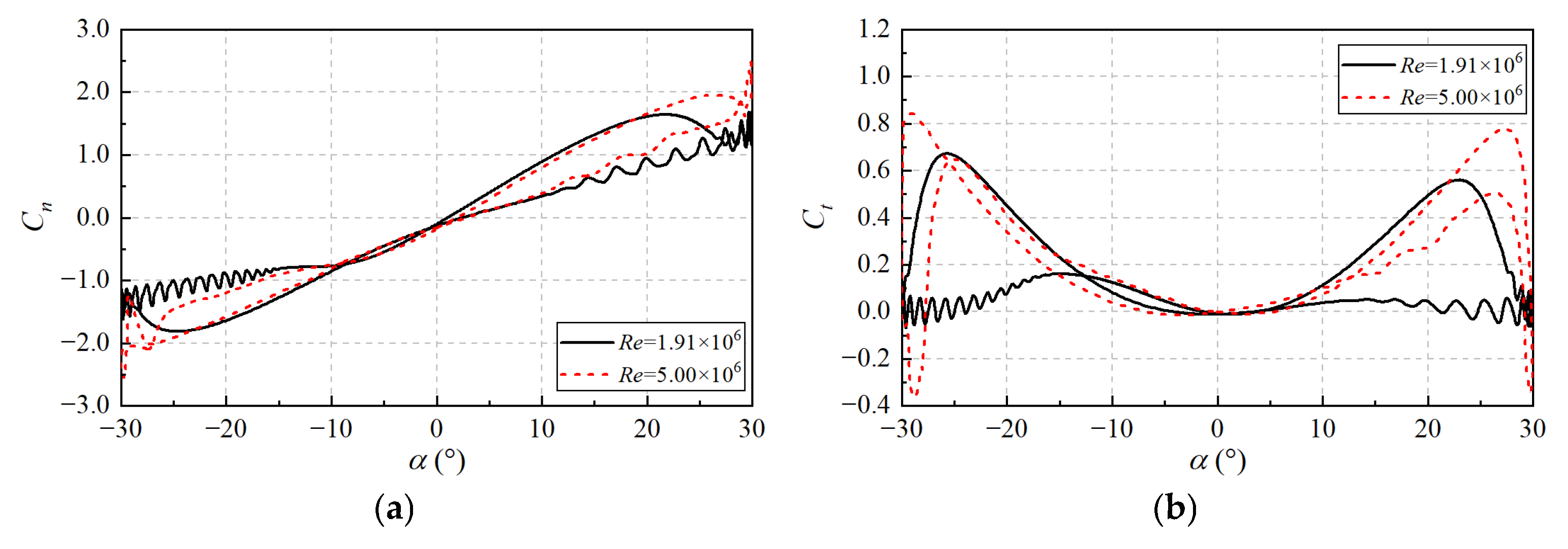
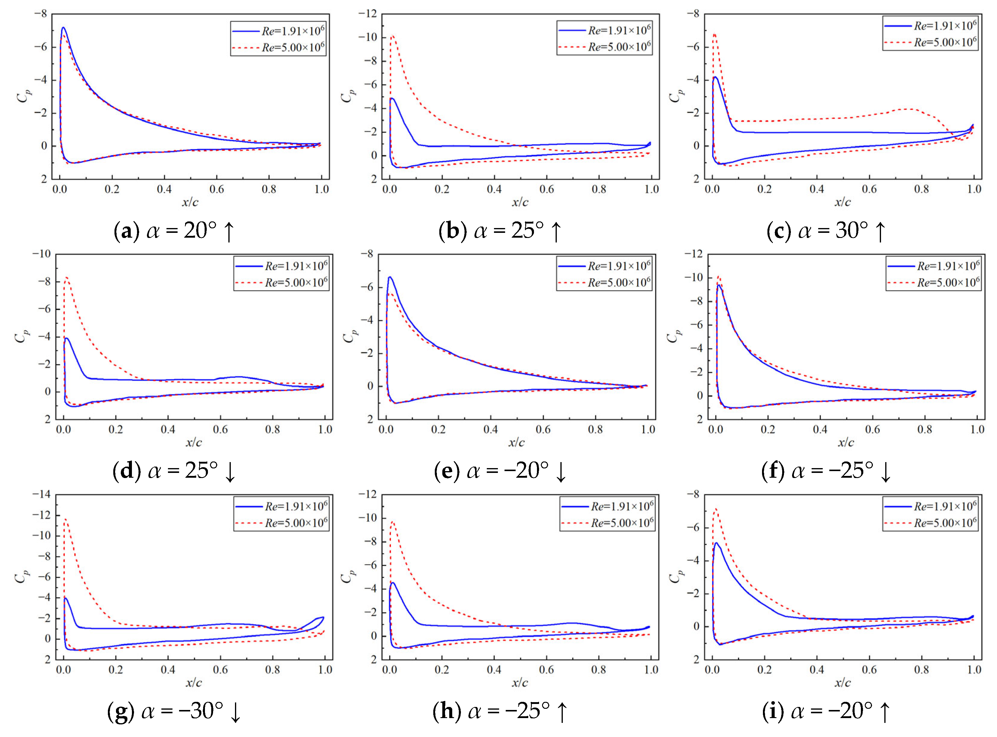
Under DPM conditions, as the angle of attack (α) increases, reverse flow originating at the trailing edge extends toward the leading edge, causing diffusion of the high-velocity regions and ultimately triggering dynamic stall at the leading edge, with a decrease in aerodynamic forces. In Phases II and IV, the leading edge fails to accumulate high-velocity flow due to the adverse flow direction relative to the pitching motion, resulting in intense aerodynamic oscillations. In Phase III, the large pitch angular velocity delays leading-edge stall, with flow separation occurring only near the trailing edge. During the decrease of α, despite the relatively low pitch angular velocity in Phase IV, the leading-edge flow recovers more effectively compared to Phase II, indicating that slower pitching facilitates aerodynamic recovery.

(ii).

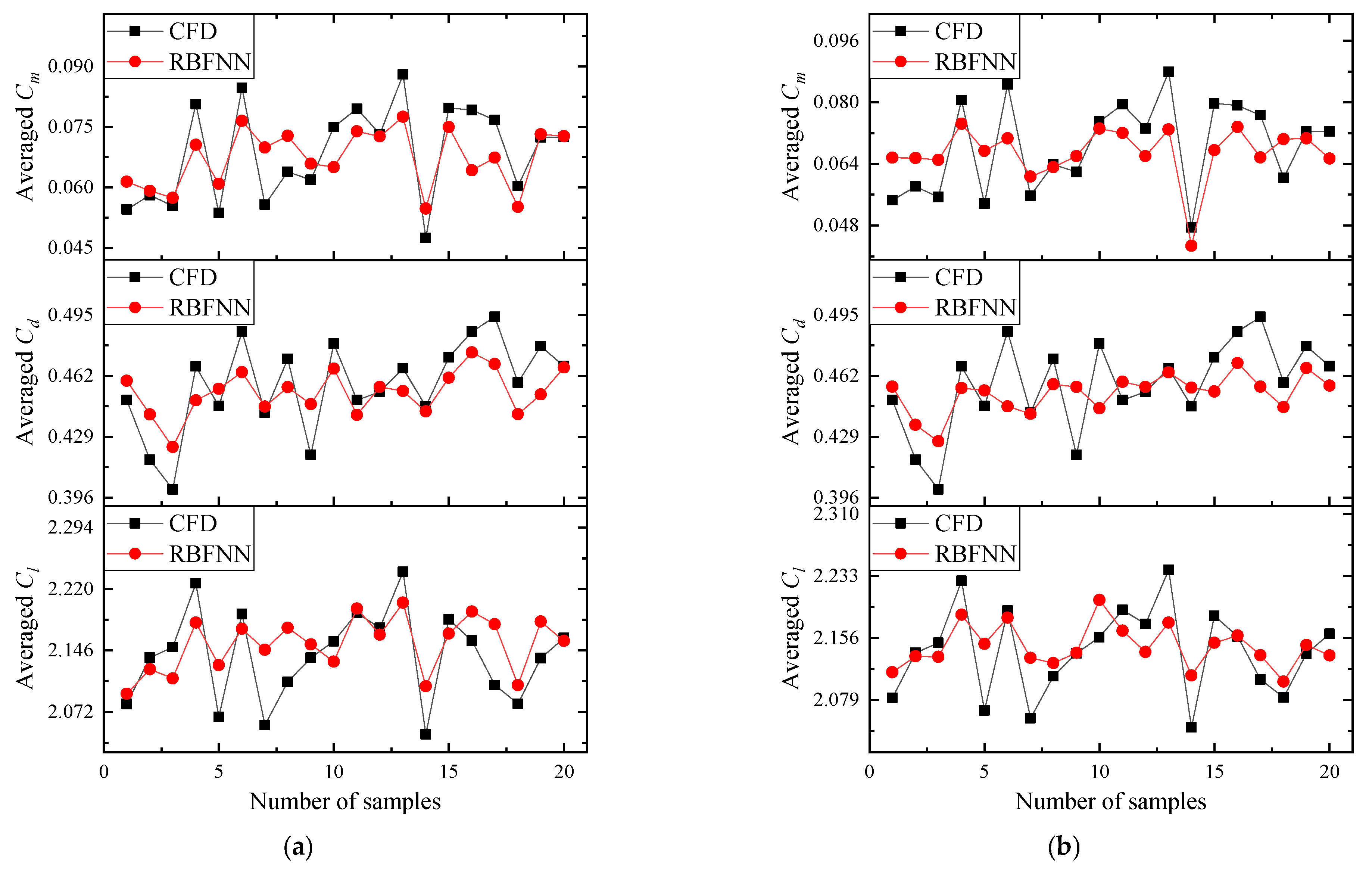
The RBFNN surrogate model, trained on 200 samples (including 20 test samples), achieves fitting accuracies of 0.982 and 0.975 (R²) for the upper and lower surfaces, respectively. This model enables the rapid prediction of aerodynamic forces based on blade geometry, making it feasible to generate a large of samples (exceeding 10⁴) required for Sobol′s sensitivity analysis.

(iii).

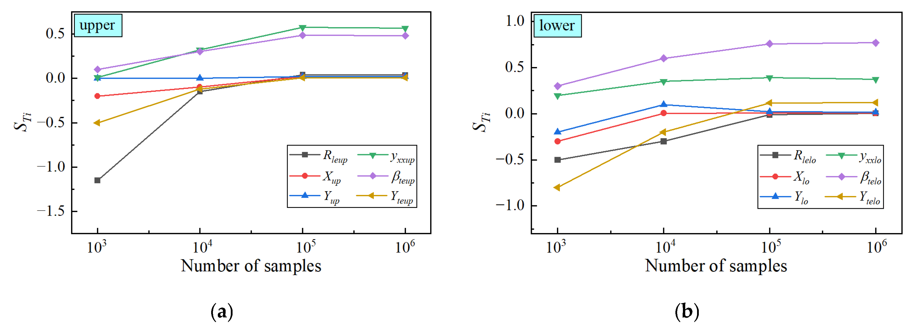
Global sensitivity analysis reveals that the curvature at the maximum thickness and the trailing-edge deflection angle are the dominant geometric parameters influencing dynamic stall behavior under DPM. Their first-order effects on aerodynamic performance are significantly greater than their interaction effects. In contrast, the leading-edge radius and location of maximum thickness exhibit relatively minor influence and should be constrained in the VAWT blade optimization process. The maximum thickness is found to significantly affect the average moment coefficient. Overall, the geometric parameters that most strongly influence DPM behavior are those shaping the mid-to-aft region of the blade, which primarily governs the surrounding flow dynamics.

7. Future Work

In this paper, DPM is simulated using the CFD method, and the global sensitivity of blade geometrical parameters on aerodynamic characteristics is analyzed. Some further work may be investigated in the future:

(i).

In this work, we study the generation and evolution of the DPM at λ = 2, and the difference in the flow field structure for different λ will be analyzed in future work.

(ii).

A global sensitivity analysis of the blade geometry parameters on the aerodynamic characteristics is performed. In a follow-up study, a sensitivity analysis of the flow conditions, such as the variation of the incoming velocity and the Reynolds number, will be introduced. This can reveal how other parameters affect the dynamic stall characteristics to better contribute to the VAWT blade design.

References

1. Leung, D.Y.C.; Yang, Y. Wind energy development and its environmental impact: A review. Renew. Sustain. Energy Rev. 2012, 16, 1031–1039. [Google Scholar] [CrossRef]
2. Keivanpour, S.; Ramudhin, A.; Ait Kadi, D. The sustainable worldwide offshore wind energy potential: A systematic review. J. Renew. Sustain. Energy 2017, 9, 065902. [Google Scholar] [CrossRef]
3. Global Wind Energy Council. Global Wind Report 2024; Global Wind Energy Council: Brussels, Belgium, 2024. [Google Scholar]
4. Rehman, S.; Rafique, M.M.; Alam, M.M.; Alhems, L.M. Vertical axis wind turbine types, efficiencies, and structural stability—A Review. Wind Struct. 2019, 29, 15–32. [Google Scholar]
5. Tjiu, W.; Marnoto, T.; Mat, S.; Ruslan, M.H.; Sopian, K. Darrieus vertical axis wind turbine for power generation I: Assessment of Darrieus VAWT configurations. Renew. Energy 2015, 75, 50–67. [Google Scholar] [CrossRef]
6. Liu, J.; Lin, H.; Zhang, J. Review on the technical perspectives and commercial viability of vertical axis wind turbines. Ocean Eng. 2019, 182, 608–626. [Google Scholar] [CrossRef]
7. Dabachi, M.A.; Rahmouni, A.; Bouksour, O. Design and aerodynamic performance of new floating H-darrieus vertical Axis wind turbines. Mater. Today Proc. 2020, 30, 899–904. [Google Scholar] [CrossRef]
8. Dabachi, M.A.; Rahmouni, A.; Rusu, E.; Bouksour, O. Aerodynamic simulations for floating darrieus-type wind turbines with three-stage rotors. Inventions 2020, 5, 18. [Google Scholar] [CrossRef]
9. Li, Q.; Maeda, T.; Kamada, Y.; Murata, J.; Furukawa, K.; Yamamoto, M. Measurement of the flow field around straight-bladed vertical axis wind turbine. J. Wind Eng. Ind. Aerodyn. 2016, 151, 70–78. [Google Scholar] [CrossRef]
10. Day, H.; Ingham, D.; Ma, L.; Pourkashanian, M. Adjoint based optimisation for efficient VAWT blade aerodynamics using CFD. J. Wind Eng. Ind. Aerodyn. 2020, 208, 104431. [Google Scholar] [CrossRef]
11. Li, Q.; Maeda, T.; Kamada, Y.; Murata, J.; Furukawa, K.; Yamamoto, M. The influence of flow field and aerodynamic forces on a straight-bladed vertical axis wind turbine. Energy 2016, 111, 260–271. [Google Scholar] [CrossRef]
12. Allet, A.; Hallé, S.; Paraschivoiu, I. Numerical simulation of dynamic stall around an airfoil in Darrieus motion. J. Sol. Energy Eng. 1999, 121, 69–76. [Google Scholar] [CrossRef]
13. Zouzou, B.; Dobrev, I.; Massouh, F.; Dizene, R. Experimental and numerical analysis of a novel Darrieus rotor with variable pitch mechanism at low TSR. Energy 2019, 186, 115832. [Google Scholar] [CrossRef]
14. Zhou, L.; Shen, X.; Ma, L.; Chen, J.; Ouyang, H.; Du, Z. Unsteady aerodynamics of the floating offshore wind turbine due to the trailing vortex induction and airfoil dynamic stall. Energy 2024, 304, 131845. [Google Scholar] [CrossRef]
15. Khalifa, N.M.; Rezaei, A.; Taha, H.E. On computational simulations of dynamic stall and its three-dimensional nature. Phys. Fluids 2023, 35, 105143. [Google Scholar] [CrossRef]
16. Dyachuk, E.; Goude, A.; Bernhoff, H. Dynamic stall modeling for the conditions of vertical axis wind turbines. AIAA J. 2014, 52, 72–81. [Google Scholar] [CrossRef]
17. Lam, H.F.; Peng, H.Y. Study of wake characteristics of a vertical axis wind turbine by two-and three-dimensional computational fluid dynamics simulations. Renew. Energy 2016, 90, 386–398. [Google Scholar] [CrossRef]
18. Leishman, J.G. Dynamic stall experiments on the NACA 23012 aerofoil. Exp. Fluids 1990, 9, 49–58. [Google Scholar] [CrossRef]
19. Tsai, H.C.; Colonius, T. Coriolis effect on dynamic stall in a vertical axis wind turbine. AIAA J. 2016, 54, 216–226. [Google Scholar] [CrossRef]
20. Brunner, C.E.; Kiefer, J.; Hultmark, M. Comparison of dynamic stall on an airfoil undergoing sinusoidal and VAWT-shaped pitch motions. In Journal of Physics: Conference Series; IOP Publishing: Bristol, UK, 2022; Volume 2265, p. 032006. [Google Scholar]
21. Hand, B.; Kelly, G.; Cashman, A. Numerical simulation of a vertical axis wind turbine airfoil experiencing dynamic stall at high Reynolds numbers. Comput. Fluids 2017, 149, 12–30. [Google Scholar] [CrossRef]
22. Iooss, B.; Lemaître, P. A review on global sensitivity analysis methods. Uncertainty management in simulation-optimization of complex systems: Algorithms and applications. In Uncertainty Management in Simulation-Optimization of Complex Systems: Algorithms and Applications; Springer: Berlin/Heidelberg, Germany, 2015; pp. 101–122. [Google Scholar]
23. Dela, A.; Shtylla, B.; de Pillis, L. Multi-method global sensitivity analysis of mathematical models. J. Theor. Biol. 2022, 546, 111159. [Google Scholar] [CrossRef]
24. Cheng, K.; Lu, Z.; Zhou, Y.; Shi, Y.; Wei, Y. Global sensitivity analysis using support vector regression. Appl. Math. Model. 2017, 49, 587–598. [Google Scholar] [CrossRef]
25. Castillo, E.; Hadi, A.S.; Conejo, A.; Fernández-Canteli, A. A general method for local sensitivity analysis with application to regression models and other optimization problems. Technometrics 2004, 46, 430–444. [Google Scholar] [CrossRef]
26. Sarrazin, F.; Pianosi, F.; Wagener, T. Global Sensitivity Analysis of environmental models: Convergence and validation. Environ. Model. Softw. 2016, 79, 135–152. [Google Scholar] [CrossRef]
27. van Griensven, A.; Meixner, T.; Grunwald, S.; Bishop, T.; Diluzio, M.; Srinivasan, R. A global sensitivity analysis tool for the parameters of multi-variable catchment models. J. Hydrol. 2006, 324, 10–23. [Google Scholar] [CrossRef]
28. Borgonovo, E.; Plischke, E. Sensitivity analysis: A review of recent advances. Eur. J. Oper. Res. 2016, 248, 869–887. [Google Scholar] [CrossRef]
29. Echeverría, F.; Mallor, F.; San Miguel, U. Global sensitivity analysis of the blade geometry variables on the wind turbine performance. Wind Energy 2017, 20, 1601–1616. [Google Scholar] [CrossRef]
30. Shum, J.G.; Lee, S. Computational Study of Airfoil Design Parameters and Sensitivity Analysis for Dynamic Stall. AIAA J. 2024, 62, 1611–1617. [Google Scholar] [CrossRef]
31. Mohamed, A.S.; Raj, L.P. Sensitivity analysis of geometric parameters on the aerodynamic performance of a multi-element airfoil. Aerosp. Sci. Technol. 2023, 132, 108074. [Google Scholar]
32. Wu, X.; Zhang, W.; Song, S. Uncertainty quantification and sensitivity analysis of transonic aerodynamics with geometric uncertainty. Int. J. Aerosp. Eng. 2017, 2017, 8107190. [Google Scholar] [CrossRef]
33. Raul, V.; Leifsson, L. Surrogate-based aerodynamic shape optimization for delaying airfoil dynamic stall using Kriging regression and infill criteria. Aerosp. Sci. Technol. 2021, 111, 106555. [Google Scholar] [CrossRef]
34. Raj, L.P.; Yee, K.; Myong, R.S. Sensitivity of ice accretion and aerodynamic performance degradation to critical physical and modeling parameters affecting airfoil icing. Aerosp. Sci. Technol. 2020, 98, 105659. [Google Scholar]
35. Rahman, S. Global sensitivity analysis by polynomial dimensional decomposition. Reliab. Eng. Syst. Saf. 2011, 96, 825–837. [Google Scholar] [CrossRef]
36. Feng, K.; Lu, Z.; Yang, C. Enhanced Morris method for global sensitivity analysis: Good proxy of Sobol’index. Struct. Multidiscip. Optim. 2019, 59, 373–387. [Google Scholar] [CrossRef]
37. Rosolem, R.; Gupta, H.V.; Shuttleworth, W.J.; Zeng, X.; de Gonçalves, L.G.G. A fully multiple-criteria implementation of the Sobol′ method for parameter sensitivity analysis. J. Geophys. Res. Atmos. 2012, 117, D07103. [Google Scholar] [CrossRef]
38. Saltelli, A.; Ratto, M.; Andres, T.; Campolongo, F.; Cariboni, J.; Gatelli, D.; Saisana, M.; Tarantola, S. Global Sensitivity Analysis: The Primer; John Wiley & Sons: Hoboken, NJ, USA, 2008. [Google Scholar]
39. Li, C.; Mahadevan, S. An efficient modularized sample-based method to estimate the first-order Sobol׳ index. Reliab. Eng. Syst. Saf. 2016, 153, 110–121. [Google Scholar] [CrossRef]
40. Wang, Y.X.; Zhang, L.L.; Liu, W.; Cheng, X.H.; Zhuang, Y.; Chronopoulos, A.T. Performance optimizations for scalable CFD applications on hybrid CPU+ MIC heterogeneous computing system with millions of cores. Comput. Fluids 2018, 173, 226–236. [Google Scholar] [CrossRef]
41. Lange, C.; Barthelmäs, P.; Rosnitschek, T.; Tremmel, S.; Rieg, F. Impact of HPC and automated CFD Simulation processes on virtual product development—A case study. Appl. Sci. 2021, 11, 6552. [Google Scholar] [CrossRef]
42. Sobieczky, H. Parametric airfoils and wings. In Recent Development of Aerodynamic Design Methodologies: Inverse Design and Optimization; Vieweg+ Teubner Verlag: Wiesbaden, Germany, 1999; pp. 71–87. [Google Scholar]
43. Della Vecchia, P.; Daniele, E.; D’Amato, E. An airfoil shape optimization technique coupling PARSEC parameterization and evolutionary algorithm. Aerosp. Sci. Technol. 2014, 32, 103–110. [Google Scholar] [CrossRef]
44. Sun, Y.B.; Meng, X.Y.; Long, T.; Wu, Y. A fast optimal Latin hypercube design method using an improved translational propagation algorithm. Eng. Optim. 2020, 52, 1244–1260. [Google Scholar] [CrossRef]
45. Li, Y.; Li, N.; Gong, G.; Yan, J. A novel design of experiment algorithm using improved evolutionary multi-objective optimization strategy. Eng. Appl. Artif. Intell. 2021, 102, 104283. [Google Scholar] [CrossRef]
46. Seshagiri, S.; Khalil, H.K. Output feedback control of nonlinear systems using RBF neural networks. IEEE Trans. Neural Netw. 2000, 11, 69–79. [Google Scholar] [CrossRef] [PubMed]
47. Li, K.; Peng, J.X.; Bai, E.W. Two-stage mixed discrete–continuous identification of radial basis function (RBF) neural models for nonlinear systems. IEEE Trans. Circuits Syst. I Regul. Pap. 2008, 56, 630–643. [Google Scholar]
48. Montazer, G.A.; Giveki, D.; Karami, M.; Rastegar, H. Radial basis function neural networks: A review. Comput. Rev. J 2018, 1, 52–74. [Google Scholar]
49. Chen, Z.; Huang, F.; Chen, W.; Zhang, J.; Sun, W.; Chen, J.; Gu, J.; Zhu, S. RBFNN-based adaptive sliding mode control design for delayed nonlinear multilateral telerobotic system with cooperative manipulation. IEEE Trans. Ind. Inform. 2019, 16, 1236–1247. [Google Scholar] [CrossRef]
50. Chicco, D.; Warrens, M.J.; Jurman, G. The coefficient of determination R-squared is more informative than SMAPE, MAE, MAPE, MSE and RMSE in regression analysis evaluation. Peerj Comput. Sci. 2021, 7, e623. [Google Scholar] [CrossRef]
51. Wickens, R.H. Wind Tunnel Investigation of Dynamic Stall of a NACA 0018 Airfoil Oscillating in Pitch; Aeronautical Note NAE-AN-27, NRC no 24262; National Aeronautical Establishment: Bedford, UK, 1985.
52. Balduzzi, F.; Bianchini, A.; Carnevale, E.A.; Ferrari, L.; Magnani, S. Feasibility analysis of a Darrieus vertical-axis wind turbine installation in the rooftop of a building. Appl. Energy 2012, 97, 921–929. [Google Scholar] [CrossRef]
53. Imran, R.M.; Hussain, D.M.A.; Soltani, M. An experimental analysis of the effect of icing on Wind turbine rotor blades. In Proceedings of the 2016 IEEE/PES Transmission and Distribution Conference and Exposition (T&D), Dallas, TX, USA, 3–5 May 2016; IEEE: Piscataway, NJ, USA, 2016; pp. 1–5. [Google Scholar]
Figure 1. The operating environment for FOWT.
Jmse 13 01327 g001
Figure 2. Velocity triangles of VAWT at different azimuth angles.
Jmse 13 01327 g002
Figure 3. Variation of α with azimuth for different TSRs.
Jmse 13 01327 g003
Figure 4. Normalized variation of VAWT blade within one cycle at different TSRs for (a) angle of attack and (b) angular velocity.
Jmse 13 01327 g004
Figure 5. The airfoil geometry and PARSEC parameters.
Jmse 13 01327 g005
Figure 6. Samples distribution in 2D space of (a) LHS and (b) OLHS methods.
Jmse 13 01327 g006
Figure 7. The three-layer network structure of RBFNN.
Jmse 13 01327 g007
Figure 8. Framework for RBFNN model construct and sensitivity analysis.
Jmse 13 01327 g008
Figure 9. Schematic of Darrieus-type pitching motion.
Jmse 13 01327 g009
Figure 10. Computational domain topology and boundary condition.
Jmse 13 01327 g010
Figure 11. Computational domain grid and detailed view.
Jmse 13 01327 g011
Figure 12. Results of aerodynamic forces for different numbers of grids of (a) Cl and (b) Cd.
Jmse 13 01327 g012
Figure 13. Results of aerodynamic forces for different time steps of (a) Cl and (b) Cd.
Jmse 13 01327 g013
Figure 14. Comparison of pressure coefficients between experimental and numerical simulations at (a) α = 20° ↑, (b) α = 30° ↑, (c) α = 20° ↓ and (d) α = −20° ↓.
Jmse 13 01327 g014
Figure 15. The four phases of variation in the angle of attack in one cycle when the TSR is 2.
Jmse 13 01327 g015
Figure 16. Aerodynamic forces of the DPM in one cycle for (a) normal force and (b) tangential force coefficients. The markers on the curves correspond to the velocity contours in Figure 16.
Jmse 13 01327 g016
Figure 17. X-velocity contour for DPM at one cycle.
Jmse 13 01327 g017
Figure 18. Comparison of different Reynolds number for (a) normal coefficient and (b) tangential coefficient.
Jmse 13 01327 g018
Figure 19. Effect of Reynolds number on airfoil pressure coefficient distribution at different angles of attack. (a) α = 20° ↑, (b) α = 25° ↑, (c) α = 30° ↑, (d) α = 25° ↓, (e) α = −20° ↓, (f) α = −25° ↓, (g) α = −30° ↓, (h) α = −25° ↑ and (i) α = −20° ↑.
Jmse 13 01327 g019
Figure 20. Comparison of predicted and CFD simulated values for (a) upper and (b) lower surfaces.
Jmse 13 01327 g020
Figure 21. Convergence of the Sobol indices of the geometry parameters for the (a) upper and (b) lower surfaces.
Jmse 13 01327 g021
Figure 22. Results of global sensitivity analysis of the geometry parameters on aerodynamic characteristics. Which (a) is Cl of upper, (b) is Cl of lower, (c) is Cd of upper, (d) is Cd of lower, (e) is Cm of upper, and (f) is Cm of lower.
Jmse 13 01327 g022