
Overview of Path Planning and Motion Control Methods for Port Transfer Vehicles


Abstract
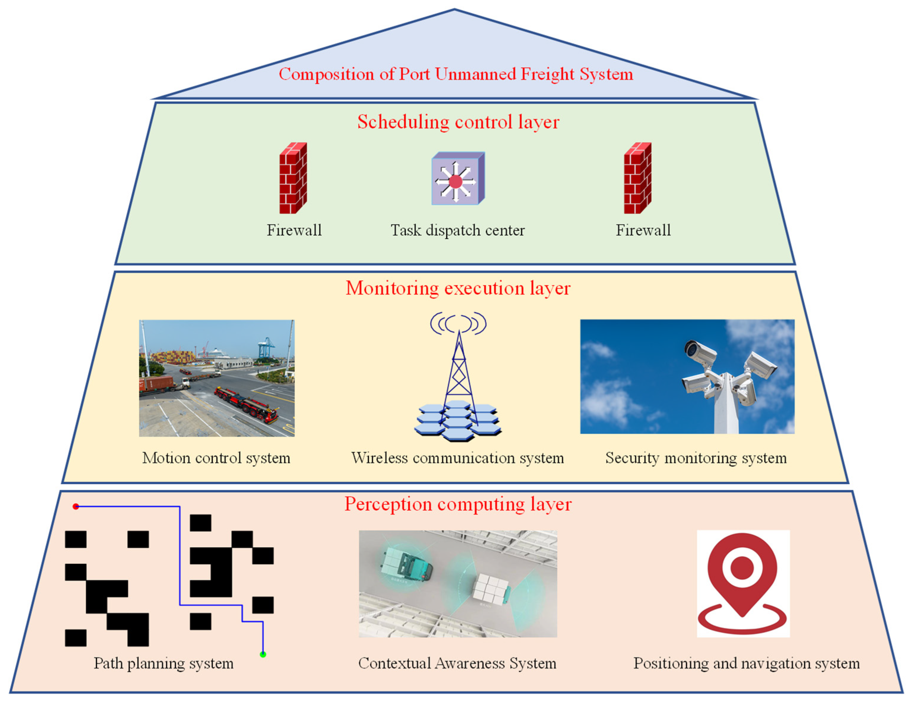
1. Introduction
2. Path Planning Algorithms for Port AIVs
2.1. Global Path Planning Method
2.1.1. Graph Search Method
2.1.2. Numerical Optimization Method
| Algorithm 1. AIVs path planning based on convex constraints in numerical optimization |
| Input: Port layout information, initial position coordinates of the AIV, target position coordinates of the AIV, static or dynamic obstacle locations Output: The optimal path from the start to the destination (sequence of path points). 1: Function AIVDynamicPathPlanning(portLayout, AIVStart, AIVGoal, obstacles): 2: convexRegions = GenerateConvexRegions(portLayout, obstacles) 3: currentPath = InitializePath(AIVStart, AIVGoal, convexRegions) 4: timeStep = 0 5: While NotReachedGoal(AIVStart, AIVGoal): 6: dynamicObstacles = UpdateDynamicObstacles(timeStep) 7: feasibleRegions = UpdateFeasibleRegions(convexRegions, dynamicObstacles) 8: optimalPath = SolveOptimizationProblem(AIVStart, AIVGoal, feasibleRegions) 9: If Not IsPathValid(optimalPath, dynamicObstacles): optimalPath = ReplanPath(AIVStart, AIVGoal, feasibleRegions) 10: AIVStart = MoveAlongPath(optimalPath, timeStep) 11: timeStep + = 1 12: Return optimal Path |
2.1.3. Intelligent Bionic Method
| Algorithm 2. AIVs path planning based on genetic algorithm |
| Input: Port layout information, number of AIVs, list of initial positions of AIVs, list of target positions of AIVs, list of obstacle positions; Output: List of optimal paths for each AIV. 1: Function GAPathPlanning(portLayout, numAIV, AIVStartPositions, AIVGoals, obstacles): 2: population = InitializePopulation(numAIV, AIVStartPositions, AIVGoals, portLayout, obstacles) 3: for generation in 1 to maxGenerations: 4: selectedPopulation = Selection(population) 5: crossedOverPopulation = Crossover(selectedPopulation) 6: mutatedPopulation = Mutation(crossedOverPopulation) 7: for individual in mutatedPopulation: 8: fitness = EvaluateFitness(individual, obstacles) 9: population = UpdatePopulation(population, mutatedPopulation) 10: bestSolution = GetBestSolution(population) 11: if CheckConvergence(bestSolution): 12: break 13: return bestSolution |
2.1.4. Intelligent Learning Optimization Method
| Algorithm 3. AIVs path planning based on particle swarm optimization algorithm |
| Input: Port layout information, number of AIVs, list of initial positions of AIVs, list of target positions of AIVs, list of obstacle positions; Output: List of optimal paths for each AIV. 1: Function PSOPathPlanning(portLayout, numAIV, AIVStartPositions, AIVGoals, obstacles): 2: particles = InitializeParticles(numAIV, AIVStartPositions, AIVGoals, portLayout, obstacles) 3: globalBest = FindGlobalBest(particles) 4: for iteration in 1 to maxIterations: 5: for particle in particles: 6: fitness = EvaluateFitness(particle, obstacles) 7: UpdatePersonalBest(particle) 8: UpdateGlobalBest(particle, globalBest) 9: UpdateVelocity(particle, globalBest) 10: UpdatePosition(particle) 11: if CheckConvergence(globalBest): 12: break 13: return globalBest |
2.2. Local Path Planning Method
2.2.1. Artificial Potential Field Method
2.2.2. Curve Optimization Method
2.2.3. Sampling-Based Method
2.2.4. Improvements and Innovations in Local Path Planning
2.2.5. Combination of Global and Local Path Planning
2.3. Multi-Vehicle Cooperative Planning
2.3.1. Multi-Agent Path Finding Algorithm
| Algorithm 4. AIVs path planning based on multi-agent path finding algorithm |
| Input: Grid map, list of agents with start positions, list of target positions, list of obstacles; Output: List of collision-free paths for each agent. 1: Function MAPF(gridMap, agents, targets, obstacles): 2: paths = InitializePaths(agents, targets) 3: openSet = InitializeOpenSet(agents) 4: while openSet is not empty: 5: agent = openSet.pop() 6: currentNode = agent.currentNode 7: if currentNode == agent.target: 8: continue // Agent has reached its target 9: neighbors = GetNeighbors(currentNode, gridMap, obstacles) 10: for neighbor in neighbors: 11: if IsCollisionFree(neighbor, paths, agent): 12: UpdatePath(agent, neighbor) 13: openSet.push(agent) 14: break 15: return paths |
2.3.2. Distributed Model Predictive Control Algorithm
| Algorithm 5. AIVs path planning based on distributed model predictive control algorithm |
| Input: System dynamics, local cost functions, constraints, initial states, prediction horizon N; Output: Optimal control inputs for each subsystem. 1: Function DMPC(systemDynamics, costFunctions, constraints, initialStates, N): 2: for each subsystem i: 3: xi(0) = initialStates[i] 4: for k = 0 to N-1: 5: ui*(k) = SolveLocalMPC(xi(k), costFunctions[i], constraints[i]) 6: Broadcast ui*(k) to neighboring subsystems 7: Receive uj*(k) from neighboring subsystems 8: xi(k+1) = UpdateState(xi(k), ui*(k), uj*(k), systemDynamics) 15: return {ui*(k)}i,k |
2.3.3. Leader–Follower Collaboration Algorithm
2.3.4. AIV Task Scheduling Algorithm
2.4. Overview and Evaluation of AIV Path Planning Methods
3. Port AIV Motion Control Algorithms
3.1. Proportional-Integral-Derivative Control
3.2. Robust Control
3.3. Sliding Mode Control
3.4. Model Predictive Control
| Algorithm 6. AIV motion control based on MPC |
| Input: Current position, motion direction, load weight, speed, and other states of the AIV; AIV kinematic model; constraints on speed, acceleration, and control inputs; cost function; desired trajectory. Output: Optimal control commands for the AIV. 1: Function MPC_AIVControl(currentState, kinematicModel, constraints, costFunction, referenceTrajectory): 2: for iteration in 1 to maxIterations: 3: predictedTrajectory = [] 4: predictedState = currentState 5: for t in 1 to N: 6: predictedState = kinematicModel(predictedState, controlInputs[t]) 7: predictedTrajectory.append(predictedState) 8: cost = costFunction(predictedTrajectory, referenceTrajectory, controlInputs) 9: if CheckConstraints(predictedTrajectory, controlInputs, constraints): 10: if cost < optimalCost: 11: optimalCost = cost 12: optimalControl = controlInputs[0] 13: controlInputs = UpdateControlInputs(controlInputs, costFunction, constraints) 14: if CheckConvergence(optimalCost): 15: break 16: return optimalControl |
3.5. Fuzzy Control
3.6. Neural Network Control
4. Development Prospects and Trends
- End-to-End Large Models: With continual advances in multimodal sensing hardware—high-resolution LiDAR, event-driven cameras, and ultra-compact inertial measurement units—end-to-end large models are poised to redefine how AIVs perceive and reason about their surroundings. Future work will focus on designing unified Transformer backbones that ingest raw point-cloud streams, vision frames, and inertial signals simultaneously, rather than in isolated pipelines. Through massive self-supervised pre-training on synthetic and real port-operation datasets, these models will learn to encode spatiotemporal patterns of cranes, vehicles, and pedestrian flows into a single, continuously updating 4D semantic representation. On top of that, emerging reinforcement-learning paradigms—such as offline RL from logged port-operation trajectories—will enable these large models to refine their decision-making policies without costly real-world trial runs. By enhancing autonomous driving technology through end-to-end lager models, RL training data can be reduced by 95%, inference speed can be increased by 600 times, and task success rate can be increased by 40% [161].
- 3D Environmental Path Planning: Traditional 2D path-planning techniques struggle in the highly cluttered, three-dimensional corridors of container terminals and automated warehouses. The next generation of AIVs will leverage dense 3D reconstructions from LiDAR and RGB-D scanners to build on-the-fly octree or voxel maps, feeding these directly into deep neural planners [162]. These planners—based on graph-convolutional networks or differentiable occupancy grids—will evaluate feasibility, clearance, and dynamic stability constraints simultaneously in full 3D. In practice, an AIV approaching a stack of high-bay racks will not only find the shortest route in the bird’s-eye view but will also judge vertical clearance margins and possible sway of suspended loads. Coupled with real-time map updates at 10 Hz, this approach promises a two-fold increase in planning robustness and a 25% reduction in dead-heading—especially critical in narrow, multi-level storage environments [163].
- Preemptive Control Based on Multi-source Sensing: As sensor miniaturization continues, low power radar chips, surface acoustic wave dust sensors, and road surface microphones will join cameras and inertial units on AIV platforms [164]. Beyond obstacle detection and localization, these heterogeneous streams will converge in a probabilistic sensor fusion engine that not only labels the scene but also infers future terrain quality and friction coefficients [165]. For instance, by correlating subtle radar echo signatures with known pothole patterns, the system can predict a rough patch 5–10 m ahead, commanding the drive controller to reduce speed and adjust suspension damping proactively [166]. Preliminary field trials suggest this “look ahead” control can reduce maintenance costs by minimizing shock loads on chassis components [167].
- Digital Twins and Virtual Debugging: Digital twin frameworks for port AIVs will evolve from static replicas to dynamic, physics informed simulation platforms [168]. By ingesting real-time telemetry—position, actuator forces, battery health—and coupling it with a high-fidelity finite element model of the vehicle, operators will be able to run “what if” analyses in milliseconds. Upcoming toolchains will integrate domain randomized virtual sensors, so that edge case scenarios can be stress tested without endangering hardware [169]. Furthermore, closed loop co-simulation with industrial PLCs (Programmable Logic Controllers) and MES (Manufacturing Execution Systems) will allow control system prototypes to be validated against digital replicas of the entire terminal. This end-to-end virtual debugging cycle will shorten commissioning times by up to 50% and enable continuous in-service calibration, ensuring that AIVs maintain peak performance even as physical infrastructure evolves [170].
5. Conclusions
Author Contributions
Funding
Conflicts of Interest
References
- Fragapane, G.; de Koster, R.; Sgarbossa, F.; Strandhagen, J.O. Planning and control of autonomous mobile robots for intralogistics: Literature review and research agenda. Eur. J. Oper. Res. 2021, 294, 405–426. [Google Scholar] [CrossRef]
- Fowler, D.S.; Mo, Y.K.; Evans, A.; Dinh-Van, S.; Ahmad, B.; Higgins, M.D.; Maple, C. A 5G Automated-Guided Vehicle SME Testbed for Resilient Future Factories. IEEE Open J. Ind. Electron. Soc. 2023, 4, 242–258. [Google Scholar] [CrossRef]
- Li, C.; Wu, W. Research on cooperative scheduling of AGV transportation and charging in intelligent warehouse system based on dynamic task chain. In Proceedings of the 2022 IEEE International Conference on Networking, Sensing and Control (ICNSC), Shanghai, China, 15–18 December 2022; pp. 1–6. [Google Scholar]
- Naeem, D.; Gheith, M.; Eltawil, A. Integrated Scheduling of AGVs and Yard Cranes in Automated Container Terminals. In Proceedings of the 2021 IEEE 8th International Conference on Industrial Engineering and Applications (ICIEA), Xi’an, China, 23–26 April 2021; pp. 632–636. [Google Scholar]
- Duan, Y.; Ren, H.; Xu, F.; Yang, X.; Meng, Y. Bi-Objective Integrated Scheduling of Quay Cranes and Automated Guided Vehicles. J. Mar. Sci. Eng. 2023, 11, 1492. [Google Scholar]
- Yang, Y.; Sun, S.; He, S.; Jiang, Y.; Wang, X.; Yin, H.; Zhu, J. Research on the Multi-Equipment Cooperative Scheduling Method of Sea-Rail Automated Container Terminals under the Loading and Unloading Mode. J. Mar. Sci. Eng. 2023, 11, 1975. [Google Scholar]
- Yang, X.; Hu, H.; Cheng, C.; Wang, Y. Automated Guided Vehicle (AGV) Scheduling in Automated Container Terminals (ACTs) Focusing on Battery Swapping and Speed Control. J. Mar. Sci. Eng. 2023, 11, 1852. [Google Scholar]
- Lu, T.; Sun, Z.H.; Qiu, S.; Ming, X. Time Window Based Genetic Algorithm for Multi-AGVs Conflict-free Path Planning in Automated Container Terminals. In Proceedings of the 2021 IEEE International Conference on Industrial Engineering and Engineering Management (IEEM), Singapore, 13–16 December 2021; pp. 603–607. [Google Scholar]
- Oyekanlu, E.A.; Smith, A.C.; Thomas, W.P.; Mulroy, G.; Hitesh, D.; Ramsey, M.; Kuhn, D.J.; Mcghinnis, J.D.; Buonavita, S.C.; Looper, N.A.; et al. A Review of Recent Advances in Automated Guided Vehicle Technologies: Integration Challenges and Research Areas for 5G-Based Smart Manufacturing Applications. IEEE Access 2020, 8, 202312–202353. [Google Scholar] [CrossRef]
- Tang, K.; Pan, X.; Guo, X.; Wu, C. A Cooperative Control Method of Differential AGV Based on Leader-Follower Strategy. In Proceedings of the 2023 42nd Chinese Control Conference (CCC), Tianjin, China, 24–26 July 2023; pp. 3012–3016. [Google Scholar]
- Ogorelysheva, N.; Vasileva, A.; Stadtler, J.; Roidl, M.; Howar, F. Mitigating Emergency Stop Collisions in AGV Fleets in Case of Control Failure. In Proceedings of the 2023 Seventh IEEE International Conference on Robotic Computing (IRC), Laguna Hills, CA, USA, 11–13 December 2023; pp. 314–322. [Google Scholar]
- Winkler, S.; Weidensager, N.; Brade, J.; Knopp, S.; Jahn, G.; Klimant, P. Use of an automated guided vehicle as a telepresence system with measurement support. In Proceedings of the 2022 IEEE 9th International Conference on Computational Intelligence and Virtual Environments for Measurement Systems and Applications (CIVEMSA), Chemnitz, Germany, 15–17 June 2022; pp. 1–6. [Google Scholar]
- Zhang, Y.; Li, B.; Sun, S.; Liu, Y.; Liang, W.; Xia, X.; Pang, Z. GCMVF-AGV: Globally Consistent Multiview Visual–Inertial Fusion for AGV Navigation in Digital Workshops. IEEE Trans. Instrum. Meas. 2023, 72, 5030116. [Google Scholar] [CrossRef]
- Xu, Y.; Qi, L.; Luan, W.; Guo, X.; Ma, H. Load-In-Load-Out AGV Route Planning in Automatic Container Terminal. IEEE Access 2020, 8, 157081–157088. [Google Scholar] [CrossRef]
- He, D.; Ouyang, B.; Fan, H.; Hu, C.; Zhang, K.; Yan, Z. Deadlock Avoidance in Closed Guide-Path Based MultiAGV Systems. IEEE Trans. Autom. Sci. Eng. 2023, 20, 2088–2098. [Google Scholar] [CrossRef]
- Zamora-Cadenas, L.; Velez, I.; Sierra-Garcia, J.E. UWB-Based Safety System for Autonomous Guided Vehicles Without Hardware on the Infrastructure. IEEE Access 2021, 9, 96430–96443. [Google Scholar] [CrossRef]
- Wang, W.; Li, J.; Bai, Z.; Wei, Z.; Peng, J. Toward Optimization of AGV Path Planning: An RRT*-ACO Algorithm. IEEE Access 2024, 12, 18387–18399. [Google Scholar] [CrossRef]
- Sha, B.; Zhu, L.; Zhu, Y.; Cheng, J. Path Planning of Agv Complex Environment Based on Ant Colony Algorithm. In Proceedings of the 2022 International Seminar on Computer Science and Engineering Technology (SCSET), Indianapolis, IN, USA, 8–9 January 2022; pp. 72–75. [Google Scholar]
- Zhang, Z.; Wu, R.; Pan, Y.; Wang, Y.; Wang, Y.; Guan, X.; Hao, J.; Zhang, J.; Li, G. A Robust Reference Path Selection Method for Path Planning Algorithm. IEEE Robot. Autom. Lett. 2022, 7, 4837–4844. [Google Scholar] [CrossRef]
- Liang, Z.; Wang, Z.; Zhao, J.; Wong, P.K.; Yang, Z.; Ding, Z. Fixed-Time and Fault-Tolerant Path-Following Control for Autonomous Vehicles With Unknown Parameters Subject to Prescribed Performance. IEEE Trans. Syst. Man Cybern. Syst. 2023, 53, 2363–2373. [Google Scholar] [CrossRef]
- Ren, Y.; Xie, X.; Li, Y. Lateral Control of Autonomous Ground Vehicles via a New Homogeneous Polynomial Parameter Dependent-Type Fuzzy Controller. IEEE Trans. Ind. Inform. 2024, 20, 11233–11241. [Google Scholar] [CrossRef]
- Lian, Y.; Xie, W.; Yang, Q.; Liu, Y.; Yang, Y.; Wu, A.G.; Eisaka, T. Improved Coding Landmark-Based Visual Sensor Position Measurement and Planning Strategy for Multiwarehouse Automated Guided Vehicle. IEEE Trans. Instrum. Meas. 2022, 71, 3509316. [Google Scholar] [CrossRef]
- Teng, S.; Hu, X.; Deng, P.; Li, B.; Li, Y.; Ai, Y.; Yang, D.; Li, L.; Xuanyuan, Z.; Zhu, F.; et al. Motion Planning for Autonomous Driving: The State of the Art and Future Perspectives. IEEE Trans. Intell. Veh. 2023, 8, 3692–3711. [Google Scholar] [CrossRef]
- Yin, J.; Li, L.; Mourelatos, Z.P.; Liu, Y.; Gorsich, D.; Singh, A.; Tau, S.; Hu, Z. Reliable Global Path Planning of Off-Road Autonomous Ground Vehicles Under Uncertain Terrain Conditions. IEEE Trans. Intell. Veh. 2024, 9, 1161–1174. [Google Scholar] [CrossRef]
- Xiang, L.; Li, X.; Liu, H.; Li, P. Parameter Fuzzy Self-Adaptive Dynamic Window Approach for Local Path Planning of Wheeled Robot. IEEE Open J. Intell. Transp. Syst. 2022, 3, 1–6. [Google Scholar] [CrossRef]
- Wang, Z.; Lu, G.; Tan, H.; Liu, M. A Risk-Field Based Motion Planning Method for Multi-Vehicle Conflict Scenario. IEEE Trans. Veh. Technol. 2024, 73, 310–322. [Google Scholar] [CrossRef]
- Ren, Z.; Rathinam, S.; Likhachev, M.; Choset, H. Multi-Objective Path-Based D* Lite. IEEE Robot. Autom. Lett. 2022, 7, 3318–3325. [Google Scholar] [CrossRef]
- Lim, W.; Lee, S.; Sunwoo, M.; Jo, K. Hybrid Trajectory Planning for Autonomous Driving in On-Road Dynamic Scenarios. IEEE Trans. Intell. Transp. Syst. 2021, 22, 341–355. [Google Scholar] [CrossRef]
- Alireza, M.; Vincent, D.; Tony, W. Experimental study of path planning problem using EMCOA for a holonomic mobile robot. J. Syst. Eng. Electron. 2021, 32, 1450–1462. [Google Scholar] [CrossRef]
- Yu, Z.; Zhu, M.; Chen, K.; Chu, X.; Wang, X. LF-Net: A Learning-Based Frenet Planning Approach for Urban Autonomous Driving. IEEE Trans. Intell. Veh. 2024, 9, 1175–1188. [Google Scholar] [CrossRef]
- Chu, L.; Gao, Z.; Dang, S.; Zhang, J.; Yu, Q. Optimization of Joint Scheduling for Automated Guided Vehicles and Unmanned Container Trucks at Automated Container Terminals Considering Conflicts. J. Mar. Sci. Eng. 2024, 12, 1190. [Google Scholar]
- Zhu, D.D.; Sun, J.Q. A New Algorithm Based on Dijkstra for Vehicle Path Planning Considering Intersection Attribute. IEEE Access 2021, 9, 19761–19775. [Google Scholar] [CrossRef]
- Lian, Y.; Xie, W.; Zhang, L. A Probabilistic Time-Constrained Based Heuristic Path Planning Algorithm in Warehouse Multi-AGV Systems. IFAC-Pap. 2020, 53, 2538–2543. [Google Scholar] [CrossRef]
- Fransen, K.J.C.; van Eekelen, J.A.W.M.; Pogromsky, A.; Boon, M.A.A.; Adan, I.J.B.F. A dynamic path planning approach for dense, large, grid-based automated guided vehicle systems. Comput. Oper. Res. 2020, 123, 105046. [Google Scholar] [CrossRef]
- Guo, K.; Zhu, J.; Shen, L. An Improved Acceleration Method Based on Multi-Agent System for AGVs Conflict-Free Path Planning in Automated Terminals. IEEE Access 2021, 9, 3326–3338. [Google Scholar] [CrossRef]
- Liu, Z.; Wang, H.; Wei, H.; Liu, M.; Liu, Y.H. Prediction, Planning, and Coordination of Thousand-Warehousing-Robot Networks With Motion and Communication Uncertainties. IEEE Trans. Autom. Sci. Eng. 2021, 18, 1705–1717. [Google Scholar] [CrossRef]
- Zhou, Y.; Huang, N. Airport AGV path optimization model based on ant colony algorithm to optimize Dijkstra algorithm in urban systems. Sustain. Comput. Inform. Syst. 2022, 35, 100716. [Google Scholar] [CrossRef]
- Singh, N.; Dang, Q.-V.; Akcay, A.; Adan, I.; Martagan, T. A matheuristic for AGV scheduling with battery constraints. Eur. J. Oper. Res. 2022, 298, 855–873. [Google Scholar] [CrossRef]
- Yang, Y.; Zhong, M.; Dessouky, Y.; Postolache, O. An integrated scheduling method for AGV routing in automated container terminals. Comput. Ind. Eng. 2018, 126, 482–493. [Google Scholar] [CrossRef]
- Zou, W.Q.; Pan, Q.K.; Wang, L.; Miao, Z.H.; Peng, C. Efficient multiobjective optimization for an AGV energy-efficient scheduling problem with release time. Knowl. Based Syst. 2022, 242, 108334. [Google Scholar]
- Gao, Y.; Chen, C.-H.; Chang, D. A Machine Learning-Based Approach for Multi-AGV Dispatching at Automated Container Terminals. J. Mar. Sci. Eng. 2023, 11, 1407. [Google Scholar]
- Sun, S.; Gu, C.; Wan, Q.; Huang, H.; Jia, X. CROTPN Based Collision-Free and Deadlock-Free Path Planning of AGVs in Logistic Center. In Proceedings of the 2018 15th International Conference on Control, Automation, Robotics and Vision (ICARCV), Singapore, 18–21 November 2018; pp. 1685–1691. [Google Scholar]
- Fanti, M.P.; Mangini, A.M.; Pedroncelli, G.; Ukovich, W. A decentralized control strategy for the coordination of AGV systems. Control Eng. Pract. 2018, 70, 86–97. [Google Scholar] [CrossRef]
- Ren, H.; Chen, S.; Yang, L.; Zhao, Y. Optimal Path Planning and Speed Control Integration Strategy for UGVs in Static and Dynamic Environments. IEEE Trans. Veh. Technol. 2020, 69, 10619–10629. [Google Scholar] [CrossRef]
- Liu, Z.; Wei, H.; Wang, H.; Li, H.; Wang, H. Integrated Task Allocation and Path Coordination for Large-Scale Robot Networks With Uncertainties. IEEE Trans. Autom. Sci. Eng. 2022, 19, 2750–2761. [Google Scholar] [CrossRef]
- Wu, Y.; Li, S.; Zhang, Q.; Sun-Woo, K.; Yan, L. Route Planning and Tracking Control of an Intelligent Automatic Unmanned Transportation System Based on Dynamic Nonlinear Model Predictive Control. IEEE Trans. Intell. Transp. Syst. 2022, 23, 16576–16589. [Google Scholar] [CrossRef]
- Ren, Z.; Rathinam, S.; Choset, H. Subdimensional Expansion for Multi-Objective Multi-Agent Path Finding. IEEE Robot. Autom. Lett. 2021, 6, 7153–7160. [Google Scholar] [CrossRef]
- Farooq, B.; Bao, J.; Raza, H.; Sun, Y.; Ma, Q. Flow-shop path planning for multi-automated guided vehicles in intelligent textile spinning cyber-physical production systems dynamic environment. J. Manuf. Syst. 2021, 59, 98–116. [Google Scholar] [CrossRef]
- Ma, J.; Ma, X.; Zang, S. Multidestination Path Planning Based on Ant Colony Decision and Rolling Control. IEEE Trans. Aerosp. Electron. Syst. 2024, 60, 8667–8681. [Google Scholar] [CrossRef]
- Zhang, J.; Wang, Z.; Han, G.; Qian, Y.; Li, Z. A Collaborative Path Planning Method for Heterogeneous Autonomous Marine Vehicles. IEEE Internet Things J. 2024, 11, 1465–1480. [Google Scholar] [CrossRef]
- Liu, W.; Zhu, X.; Wang, L.; Wang, S. Multiple equipment scheduling and AGV trajectory generation in U-shaped sea-rail intermodal automated container terminal. Measurement 2023, 206, 112262. [Google Scholar] [CrossRef]
- Li, D.; Wang, L.; Cai, J.; Ma, K.; Tan, T. Research on Terminal Distance Index-Based Multi-Step Ant Colony Optimization for Mobile Robot Path Planning. IEEE Trans. Autom. Sci. Eng. 2023, 20, 2321–2337. [Google Scholar] [CrossRef]
- Wang, J.; Yuan, X.; Huang, G.; Tan, W.; Wang, Y. Multi-Race Ant Colony Parallel Chaos Search Method for Path Planning on 3-D Terrain Considering Energy Consumption and Travel Distance. IEEE Trans. Veh. Technol. 2024, 73, 16201–16211. [Google Scholar] [CrossRef]
- Liu, J.; Wei, X.; Huang, H. An Improved Grey Wolf Optimization Algorithm and its Application in Path Planning. IEEE Access 2021, 9, 121944–121956. [Google Scholar] [CrossRef]
- Zhang, Q.; Zhao, J.; Pan, L.; Wu, X.; Hou, Y.; Qi, X. Optimal Path Planning for Mobile Robots in Complex Environments Based on the Gray Wolf Algorithm and Self-Powered Sensors. IEEE Sens. J. 2023, 23, 20756–20765. [Google Scholar] [CrossRef]
- Lin, S.; Liu, A.; Wang, J.; Kong, X. An intelligence-based hybrid PSO-SA for mobile robot path planning in warehouse. J. Comput. Sci. 2023, 67, 101938. [Google Scholar] [CrossRef]
- Zhang, J.; Li, Z.; Li, L.; Li, Y.; Dong, H.-r. A bi-level cooperative operation approach for AGV based automated valet parking. Transp. Res. Part C Emerg. Technol. 2021, 128, 103140. [Google Scholar]
- Julius Fusic, S.; Kanagaraj, G.; Hariharan, K.; Karthikeyan, S. Optimal path planning of autonomous navigation in outdoor environment via heuristic technique. Transp. Res. Interdiscip. Perspect. 2021, 12, 100473. [Google Scholar] [CrossRef]
- Li, F.; Cheng, J.; Mao, Z.; Wang, Y.; Feng, P. Enhancing Safety and Efficiency in Automated Container Terminals: Route Planning for Hazardous Material AGV Using LSTM Neural Network and Deep Q-Network. J. Intell. Connect. Veh. 2024, 7, 64–77. [Google Scholar] [CrossRef]
- Zhang, L.; Zhang, Y.; Li, Y. Mobile Robot Path Planning Based on Improved Localized Particle Swarm Optimization. IEEE Sens. J. 2021, 21, 6962–6972. [Google Scholar] [CrossRef]
- Jian, Z.; Zhang, S.; Chen, S.; Nan, Z.; Zheng, N. A Global-Local Coupling Two-Stage Path Planning Method for Mobile Robots. IEEE Robot. Autom. Lett. 2021, 6, 5349–5356. [Google Scholar] [CrossRef]
- Kumar, L.; Sadhu, A.K.; Dasgupta, R. Simultaneous Learning and Planning Within Sensing Range: An Approach for Local Path Planning. IEEE Trans. Artif. Intell. 2024, 5, 6399–6411. [Google Scholar] [CrossRef]
- Pan, Z.; Zhang, C.; Xia, Y.; Xiong, H.; Shao, X. An Improved Artificial Potential Field Method for Path Planning and Formation Control of the Multi-UAV Systems. IEEE Trans. Circuits Syst. II Express Briefs 2022, 69, 1129–1133. [Google Scholar] [CrossRef]
- Lu, M.K.; Ge, M.F.; Ding, T.F.; Zhong, L.; Liu, Z.W. Hierarchical Piecewise-Trajectory Planning Framework for Autonomous Ground Vehicles Considering Motion Limitation and Energy Consumption. IEEE Internet Things J. 2024, 11, 30145–30160. [Google Scholar] [CrossRef]
- Zhang, T.; Wang, J.; Meng, M.Q.H. Generative Adversarial Network Based Heuristics for Sampling-Based Path Planning. IEEE/CAA J. Autom. Sin. 2022, 9, 64–74. [Google Scholar] [CrossRef]
- Li, H.; Liu, W.; Yang, C.; Wang, W.; Qie, T.; Xiang, C. An Optimization-Based Path Planning Approach for Autonomous Vehicles Using the DynEFWA-Artificial Potential Field. IEEE Trans. Intell. Veh. 2022, 7, 263–272. [Google Scholar] [CrossRef]
- Zheng, X.; Li, H.; Zhang, Q.; Liu, Y.; Chen, X.; Liu, H.; Luo, T.; Gao, J.; Xia, L. Intelligent Decision-Making Method for Vehicles in Emergency Conditions Based on Artificial Potential Fields and Finite State Machines. J. Intell. Connect. Veh. 2024, 7, 19–29. [Google Scholar] [CrossRef]
- Szczepanski, R.; Tarczewski, T.; Erwinski, K. Energy Efficient Local Path Planning Algorithm Based on Predictive Artificial Potential Field. IEEE Access 2022, 10, 39729–39742. [Google Scholar] [CrossRef]
- Chen, X.; Liu, S.; Zhao, J.; Wu, H.; Xian, J.; Montewka, J. Autonomous port management based AGV path planning and optimization via an ensemble reinforcement learning framework. Ocean Coast. Manag. 2024, 251, 107087. [Google Scholar] [CrossRef]
- Wang, Z.; Zhao, X.; Zhang, J.; Yang, N.; Wang, P.; Tang, J.; Zhang, J.; Shi, L. APF-CPP: An Artificial Potential Field Based Multi-Robot Online Coverage Path Planning Approach. IEEE Robot. Autom. Lett. 2024, 9, 9199–9206. [Google Scholar] [CrossRef]
- Heinemann, T.; Riedel, O.; Lechler, A. Generating Smooth Trajectories in Local Path Planning for Automated Guided Vehicles in Production. Procedia Manuf. 2019, 39, 98–105. [Google Scholar] [CrossRef]
- Liu, Y.; Wang, L. AGV Path Planning: An Improved A* Algorithm Based on Bézier Curve Smoothing. In Proceedings of the 2024 39th Youth Academic Annual Conference of Chinese Association of Automation (YAC), Dalian, China, 7–9 June 2024; pp. 243–247. [Google Scholar]
- Zhao, B.; Shao, S.; Lei, L.; Wang, X.; Yang, X.; Wang, Q.; Hu, Y. Curve Fitting-Based Dynamic Path Planning and Tracking Control for Flexible Needle Insertion. IEEE Trans. Med. Robot. Bionics 2022, 4, 436–447. [Google Scholar] [CrossRef]
- Song, X.; Gao, H.; Ding, T.; Gu, Y.; Liu, J.; Tian, K. A Review of the Motion Planning and Control Methods for Automated Vehicles. Sensors 2023, 23, 6140. [Google Scholar] [CrossRef]
- Lin, P.; Javanmardi, E.; Tsukada, M. Clothoid Curve-Based Emergency-Stopping Path Planning With Adaptive Potential Field for Autonomous Vehicles. IEEE Trans. Veh. Technol. 2024, 73, 9747–9762. [Google Scholar] [CrossRef]
- Long, C.; Dongfang, Q.; Xing, X.; Yingfeng, C.; Ju, X. A path and velocity planning method for lane changing collision avoidance of intelligent vehicle based on cubic 3-D Bezier curve. Adv. Eng. Softw. 2019, 132, 65–73. [Google Scholar]
- You, C.; Lu, J.; Filev, D.; Tsiotras, P. Autonomous Planning and Control for Intelligent Vehicles in Traffic. IEEE Trans. Intell. Transp. Syst. 2020, 21, 2339–2349. [Google Scholar] [CrossRef]
- Bulut, V. Path planning for autonomous ground vehicles based on quintic trigonometric Bézier curve. J. Braz. Soc. Mech. Sci. Eng. 2021, 43, 104. [Google Scholar] [CrossRef]
- Wu, Y.; Li, X.; Gao, J.; Yang, X. Research on Automatic Vertical Parking Path-Planning Algorithms for Narrow Parking Spaces. Electronics 2023, 12, 4203. [Google Scholar] [CrossRef]
- Yang, X.; Zhu, X.; Liu, W.; Ye, H.; Xue, W.; Yan, C.; Xu, W. A Hybrid Autonomous Recovery Scheme for AUV Based Dubins Path and Non-Singular Terminal Sliding Mode Control Method. IEEE Access 2022, 10, 61265–61276. [Google Scholar] [CrossRef]
- Essuman, J.B.; Meng, X. Optimal Trajectory Planning for Autonomous Vehicles in Unstructured Environments. IEEE Control Syst. Lett. 2024, 8, 2673–2678. [Google Scholar] [CrossRef]
- Yao, Y.; Huang, X.; Huang, D.; Tian, C. Research on adaptive multi segment arc parking path fitting algorithm. In Proceedings of the 2023 3rd International Conference on Consumer Electronics and Computer Engineering (ICCECE), Guangzhou, China, 6–8 January 2023; pp. 362–367. [Google Scholar]
- Wang, J.; Jia, X.; Zhang, T.; Ma, N.; Meng, M.Q.H. Deep Neural Network Enhanced Sampling-Based Path Planning in 3D Space. IEEE Trans. Autom. Sci. Eng. 2022, 19, 3434–3443. [Google Scholar] [CrossRef]
- Qi, J.; Yang, H.; Sun, H. MOD-RRT*: A Sampling-Based Algorithm for Robot Path Planning in Dynamic Environment. IEEE Trans. Ind. Electron. 2021, 68, 7244–7251. [Google Scholar] [CrossRef]
- Francis, A.; Faust, A.; Chiang, H.T.L.; Hsu, J.; Kew, J.C.; Fiser, M.; Lee, T.W.E. Long-Range Indoor Navigation With PRM-RL. IEEE Trans. Robot. 2020, 36, 1115–1134. [Google Scholar] [CrossRef]
- Wang, X.; Wei, J.; Zhou, X.; Xia, Z.; Gu, X. AEB-RRT*: An adaptive extension bidirectional RRT* algorithm. Auton. Robot. 2022, 46, 685–704. [Google Scholar] [CrossRef]
- Novosad, M.; Penicka, R.; Vonasek, V. CTopPRM: Clustering Topological PRM for Planning Multiple Distinct Paths in 3D Environments. IEEE Robot. Autom. Lett. 2023, 8, 7336–7343. [Google Scholar] [CrossRef]
- Jiang, C.; Hu, Z.; Mourelatos, Z.P.; Gorsich, D.; Jayakumar, P.; Fu, Y.; Majcher, M. R2-RRT*: Reliability-Based Robust Mission Planning of Off-Road Autonomous Ground Vehicle Under Uncertain Terrain Environment. IEEE Trans. Autom. Sci. Eng. 2022, 19, 1030–1046. [Google Scholar] [CrossRef]
- Ma, H.; Meng, F.; Ye, C.; Wang, J.; Meng, M.Q.H. Bi-Risk-RRT Based Efficient Motion Planning for Autonomous Ground Vehicles. IEEE Trans. Intell. Veh. 2022, 7, 722–733. [Google Scholar] [CrossRef]
- Zhang, R.; Chai, R.; Chen, K.; Zhang, J.; Chai, S.; Xia, Y.; Tsourdos, A. Efficient and Near-Optimal Global Path Planning for AGVs: A DNN-Based Double Closed-Loop Approach With Guarantee Mechanism. IEEE Trans. Ind. Electron. 2024, 72, 681–692. [Google Scholar] [CrossRef]
- Fan, H.; Zhu, F.; Liu, C.; Zhang, L.; Zhuang, L.; Li, D.; Zhu, W.; Hu, J.; Li, H.; Kong, Q. Baidu Apollo EM Motion Planner. arXiv 2018, arXiv:1807.08048. [Google Scholar]
- Ding, W.; Zhang, L.; Chen, J.; Shen, S. Safe Trajectory Generation for Complex Urban Environments Using Spatio-Temporal Semantic Corridor. IEEE Robot. Autom. Lett. 2019, 4, 2997–3004. [Google Scholar] [CrossRef]
- Li, B.; Ouyang, Y.; Li, X.; Cao, D.; Zhang, T.; Wang, Y. Mixed-Integer and Conditional Trajectory Planning for an Autonomous Mining Truck in Loading/Dumping Scenarios: A Global Optimization Approach. IEEE Trans. Intell. Veh. 2023, 8, 1512–1522. [Google Scholar] [CrossRef]
- Li, B.; Wang, Y.; Ma, S.; Bian, X.; Li, H.; Zhang, T.; Li, X.; Zhang, Y. Adaptive Pure Pursuit: A Real-Time Path Planner Using Tracking Controllers to Plan Safe and Kinematically Feasible Paths. IEEE Trans. Intell. Veh. 2023, 8, 4155–4168. [Google Scholar] [CrossRef]
- Wang, N.; Xu, H. Dynamics-Constrained Global-Local Hybrid Path Planning of an Autonomous Surface Vehicle. IEEE Trans. Veh. Technol. 2020, 69, 6928–6942. [Google Scholar] [CrossRef]
- Wen, J.; Zhang, X.; Gao, H.; Yuan, J.; Fang, Y. E3MoP: Efficient Motion Planning Based on Heuristic-Guided Motion Primitives Pruning and Path Optimization With Sparse-Banded Structure. IEEE Trans. Autom. Sci. Eng. 2022, 19, 2762–2775. [Google Scholar] [CrossRef]
- Li, H.; Zhao, T.; Dian, S. Forward search optimization and subgoal-based hybrid path planning to shorten and smooth global path for mobile robots. Knowl. Based Syst. 2022, 258, 110034. [Google Scholar] [CrossRef]
- Huang, Z.; Chu, D.; Wu, C.; He, Y. Path Planning and Cooperative Control for Automated Vehicle Platoon Using Hybrid Automata. IEEE Trans. Intell. Transp. Syst. 2019, 20, 959–974. [Google Scholar] [CrossRef]
- Iris, Ç.; Lam, J.S.L. A review of energy efficiency in ports: Operational strategies, technologies and energy management systems. Renew. Sustain. Energy Rev. 2019, 112, 170–182. [Google Scholar] [CrossRef]
- Iris, Ç.; Christensen, J.; Pacino, D.; Ropke, S. Flexible ship loading problem with transfer vehicle assignment and scheduling. Transp. Res. Part B: Methodol. 2018, 111, 113–134. [Google Scholar] [CrossRef]
- Ren, Z.; Rathinam, S.; Choset, H. CBSS: A New Approach for Multiagent Combinatorial Path Finding. IEEE Trans. Robot. 2023, 39, 2669–2683. [Google Scholar] [CrossRef]
- An, G.; Talebpour, A. Vehicle Platooning for Merge Coordination in a Connected Driving Environment: A Hybrid ACC-DMPC Approach. IEEE Trans. Intell. Transp. Syst. 2023, 24, 5239–5248. [Google Scholar] [CrossRef]
- Zhang, B.; Huang, J.; Su, Y.; Wang, X.; Chen, Y.H.; Yang, D.; Zhong, Z. Safety-Guaranteed Oversized Cargo Cooperative Transportation With Closed-Form Collision-Free Trajectory Generation and Tracking Control. IEEE Trans. Intell. Transp. Syst. 2024, 25, 20162–20174. [Google Scholar] [CrossRef]
- Hönig, W.; Kiesel, S.; Tinka, A.; Durham, J.W.; Ayanian, N. Persistent and Robust Execution of MAPF Schedules in Warehouses. IEEE Robot. Autom. Lett. 2019, 4, 1125–1131. [Google Scholar] [CrossRef]
- Skrynnik, A.; Andreychuk, A.; Yakovlev, K.; Panov, A.I. When to Switch: Planning and Learning for Partially Observable Multi-Agent Pathfinding. IEEE Trans. Neural Netw. Learn. Syst. 2024, 35, 17411–17424. [Google Scholar] [CrossRef] [PubMed]
- Hua, Y.; Wang, Y.; Ji, Z. Adaptive Lifelong Multi-Agent Path Finding With Multiple Priorities. IEEE Robot. Autom. Lett. 2024, 9, 5607–5614. [Google Scholar] [CrossRef]
- Mi, X.; Zou, Y.; Li, S.; Karimi, H.R. Self-Triggered DMPC Design for Cooperative Multiagent Systems. IEEE Trans. Ind. Electron. 2020, 67, 512–520. [Google Scholar] [CrossRef]
- Wei, H.; Zhang, K.; Shi, Y. Self-Triggered Min–Max DMPC for Asynchronous Multiagent Systems With Communication Delays. IEEE Trans. Ind. Inform. 2022, 18, 6809–6817. [Google Scholar] [CrossRef]
- Cai, Y.; Li, Y.; Lian, Y.; Chen, L.; Zhong, Y.; Sun, X.; Yuan, C. Cooperative Control of Coupled Multiagent System of Autonomous Vehicle Chassis Based on Co-DMPC. IEEE Trans. Transp. Electrif. 2025, 11, 1875–1890. [Google Scholar] [CrossRef]
- Ning, B.; Han, Q.L.; Lu, Q. Fixed-Time Leader-Following Consensus for Multiple Wheeled Mobile Robots. IEEE Trans. Cybern. 2020, 50, 4381–4392. [Google Scholar] [CrossRef]
- An, L.; Yang, G.H.; Deng, C.; Wen, C. Event-Triggered Reference Governors for Collisions-Free Leader–Following Coordination Under Unreliable Communication Topologies. IEEE Trans. Autom. Control 2024, 69, 2116–2130. [Google Scholar] [CrossRef]
- Wang, J.; Zhang, H.; Wang, Z.; Fu, J.; Wang, W.; Meng, Q. Event-Triggered Leader-Following Consensus Control of Nonlinear Multiagent Systems With Generally Uncertain Markovian Switching Topologies. IEEE Trans. Syst. Man Cybern. Syst. 2024, 54, 4942–4954. [Google Scholar] [CrossRef]
- Li, Z.; Pan, Q.; Miao, Z.; Sang, H.; Li, W. Automated Guided Vehicle Scheduling Problem in Manufacturing Workshops: An Adaptive Parallel Evolutionary Algorithm. IEEE Trans. Autom. Sci. Eng. 2025, 22, 7361–7372. [Google Scholar] [CrossRef]
- Wu, Y.; Zhu, X.; Fei, J.; Xu, H. A Novel Joint Optimization Method of Multi-Agent Task Offloading and Resource Scheduling for Mobile Inspection Service in Smart Factory. IEEE Trans. Veh. Technol. 2024, 73, 8563–8575. [Google Scholar] [CrossRef]
- Wei, Q.; Yan, Y.; Zhang, J.; Xiao, J.; Wang, C. A Self-Attention-Based Deep Reinforcement Learning Approach for AGV Dispatching Systems. IEEE Trans. Neural Netw. Learn. Syst. 2024, 35, 7911–7922. [Google Scholar] [CrossRef] [PubMed]
- Li, Z.; Sang, H.; Pan, Q.; Gao, K.; Han, Y.; Li, J. Dynamic AGV Scheduling Model With Special Cases in Matrix Production Workshop. IEEE Trans. Ind. Inform. 2023, 19, 7762–7770. [Google Scholar] [CrossRef]
- Sierra-García, J.E.; Santos, M. AGV fuzzy control optimized by genetic algorithms. Log. J. IGPL 2024, 32, 955–970. [Google Scholar]
- Liu, W.; Li, M.; Liu, C. AGV Dual-wheel Speed Synchronous Control based on Adaptive Fuzzy PID. In Proceedings of the 2022 IEEE 5th Advanced Information Management, Communicates, Electronic and Automation Control Conference (IMCEC), Chongqing, China, 16–18 December 2022; pp. 564–569. [Google Scholar]
- Xin, M.; Yin, Y.; Zhang, K.; Lackner, D.; Ren, Z.; Minor, M. Continuous Robust Trajectory Tracking Control for Autonomous Ground Vehicles Considering Lateral and Longitudinal Kinematics and Dynamics via Recursive Backstepping. In Proceedings of the 2021 IEEE/RSJ International Conference on Intelligent Robots and Systems (IROS), Prague, Czech Republic, 27 September–1 October 2021; pp. 8373–8380. [Google Scholar]
- Gao, Z.; Zhang, Y.; Guo, G. Fixed-Time Prescribed Performance Adaptive Fixed-Time Sliding Mode Control for Vehicular Platoons With Actuator Saturation. IEEE Trans. Intell. Transp. Syst. 2022, 23, 24176–24189. [Google Scholar] [CrossRef]
- Liu, W.; He, C.; Ji, Y.; Hou, X.; Zhang, J. Active Disturbance Rejection Control of Path Following Control for Autonomous Ground Vehicles. In Proceedings of the 2020 Chinese Automation Congress (CAC), Shanghai, China, 6–8 November 2020; pp. 6839–6844. [Google Scholar]
- Zhou, X.; Jin, L.; Liu, Y. Modeling and Simulation Research of Heavy-duty AGV Tracking Control System Based on Magnetic Navigation. J. Phys. Conf. Ser. 2021, 1746, 012021. [Google Scholar] [CrossRef]
- Taghavifar, H. Neural Network Autoregressive With Exogenous Input Assisted Multi-Constraint Nonlinear Predictive Control of Autonomous Vehicles. IEEE Trans. Veh. Technol. 2019, 68, 6293–6304. [Google Scholar] [CrossRef]
- Zhao, D.; Wang, Z.; Liu, S.; Han, Q.L.; Wei, G. PID Tracking Control Under Multiple Description Encoding Mechanisms. IEEE Trans. Syst. Man Cybern. Syst. 2023, 53, 7025–7037. [Google Scholar] [CrossRef]
- Fu, W.; Liu, Y.; Zhang, X. Research on Accurate Motion Trajectory Control Method of Four-Wheel Steering AGV Based on Stanley-PID Control. Sensors 2023, 23, 7219. [Google Scholar] [PubMed]
- Anil, A.; Jisha, V.R. Trajectory Tracking Control of an Autonomous Vehicle using Model Predictive Control and PID Controller. In Proceedings of the 2023 International Conference on Control, Communication and Computing (ICCC), Thiruvananthapuram, India, 19–21 May 2023; pp. 1–6. [Google Scholar]
- Moshayedi, A.J.; Li, J.; Sina, N.; Chen, X.; Liao, L.; Gheisari, M.; Xie, X. Simulation and Validation of Optimized PID Controller in AGV (Automated Guided Vehicles) Model Using PSO and BAS Algorithms. Comput. Intell. Neurosci. 2022, 2022, 7799654. [Google Scholar] [CrossRef] [PubMed]
- Shi, Q.; Zhang, H. Road-Curvature-Range-Dependent Path Following Controller Design for Autonomous Ground Vehicles Subject to Stochastic Delays. IEEE Trans. Intell. Transp. Syst. 2022, 23, 17440–17450. [Google Scholar] [CrossRef]
- Chen, B.S.; Liu, H.T.; Wu, R.S. Robust H∞ Fault-Tolerant Observer-Based PID Path Tracking Control of Autonomous Ground Vehicle With Control Saturation. IEEE Open J. Veh. Technol. 2024, 5, 298–311. [Google Scholar] [CrossRef]
- Jin, X.; Yu, Z.; Yin, G.; Wang, J. Improving Vehicle Handling Stability Based on Combined AFS and DYC System via Robust Takagi-Sugeno Fuzzy Control. IEEE Trans. Intell. Transp. Syst. 2018, 19, 2696–2707. [Google Scholar] [CrossRef]
- Sariyildiz, E.; Oboe, R.; Ohnishi, K. Disturbance Observer-Based Robust Control and Its Applications: 35th Anniversary Overview. IEEE Trans. Ind. Electron. 2020, 67, 2042–2053. [Google Scholar] [CrossRef]
- Shin, J.; Kwak, D.; Lee, T. Robust path control for an autonomous ground vehicle in rough terrain. Control Eng. Pract. 2020, 98, 104384. [Google Scholar] [CrossRef]
- Lee, M.Y.; Chen, B.S. Robust H∞ Network Observer-Based Attack-Tolerant Path Tracking Control of Autonomous Ground Vehicle. IEEE Access 2022, 10, 58332–58353. [Google Scholar] [CrossRef]
- Xu, Y.; Wu, Z.G.; Pan, Y.J. Perceptual Interaction-Based Path Tracking Control of Autonomous Vehicles Under DoS Attacks: A Reinforcement Learning Approach. IEEE Trans. Veh. Technol. 2023, 72, 14028–14039. [Google Scholar] [CrossRef]
- Liang, Z.; Zhao, J.; Liu, B.; Wang, Y.; Ding, Z. Velocity-Based Path Following Control for Autonomous Vehicles to Avoid Exceeding Road Friction Limits Using Sliding Mode Method. IEEE Trans. Intell. Transp. Syst. 2022, 23, 1947–1958. [Google Scholar] [CrossRef]
- Qiang, Z.; Li, W.F.; Zhou, J.L. No-Load Formation Control of Dual AGVs Based on Container Terminals. In Proceedings of the 2022 IEEE International Conference on Networking, Sensing and Control (ICNSC), Shanghai, China, 15–18 December 2022; pp. 1–5. [Google Scholar]
- Zhong, Z.; Wang, X.; Lam, H.K. Finite-Time Fuzzy Sliding Mode Control for Nonlinear Descriptor Systems. IEEE/CAA J. Autom. Sin. 2021, 8, 1141–1152. [Google Scholar] [CrossRef]
- El Hajjami, L.; Mellouli, E.M.; Berrada, M. Robust adaptive non-singular fast terminal sliding-mode lateral control for an uncertain ego vehicle at the lane-change maneuver subjected to abrupt change. Int. J. Dyn. Control 2021, 9, 1765–1782. [Google Scholar] [CrossRef]
- Jiang, B.; Li, J.; Yang, S. An improved sliding mode approach for trajectory following control of nonholonomic mobile AGV. Sci. Rep. 2022, 12, 17763. [Google Scholar] [CrossRef]
- Chen, Z.; Pan, S.; Tang, X.; Meng, X.; Gao, W.; Yu, B. Design and application of finite-time tracking control for autonomous ground vehicle affected by external disturbances. Int. J. Robust Nonlinear Control 2024, 34, 12257–12285. [Google Scholar] [CrossRef]
- Li, X.; Sun, Z.; Cao, D.; Liu, D.; He, H. Development of a new integrated local trajectory planning and tracking control framework for autonomous ground vehicles. Mech. Syst. Signal Process. 2017, 87, 118–137. [Google Scholar] [CrossRef]
- Cheng, S.; Li, L.; Chen, X.; Wu, J.; Wang, H.d. Model-Predictive-Control-Based Path Tracking Controller of Autonomous Vehicle Considering Parametric Uncertainties and Velocity-Varying. IEEE Trans. Ind. Electron. 2021, 68, 8698–8707. [Google Scholar] [CrossRef]
- Qi, J.; Wu, Y. Trajectory Tracking Control for Double-steering Automated Guided Vehicle Based on Model Predictive Control. J. Phys. Conf. Ser. 2020, 1449, 012107. [Google Scholar] [CrossRef]
- Tang, M.; Lin, S.; Luo, Y. Mecanum Wheel AGV Trajectory Tracking Control Based on Efficient MPC Algorithm. IEEE Access 2024, 12, 13763–13772. [Google Scholar] [CrossRef]
- Zhang, K.; Sun, Q.; Shi, Y. Trajectory Tracking Control of Autonomous Ground Vehicles Using Adaptive Learning MPC. IEEE Trans. Neural Netw. Learn. Syst. 2021, 32, 5554–5564. [Google Scholar] [CrossRef]
- Liu, X.; Wang, G.; Chen, K. Nonlinear Model Predictive Tracking Control With C/GMRES Method for Heavy-Duty AGVs. IEEE Trans. Veh. Technol. 2021, 70, 12567–12580. [Google Scholar] [CrossRef]
- Li, J.; Ran, M.; Xie, L. Design and Experimental Evaluation of a Hierarchical Controller for an Autonomous Ground Vehicle With Large Uncertainties. IEEE Trans. Control Syst. Technol. 2022, 30, 1215–1227. [Google Scholar] [CrossRef]
- He, F.; Huang, Q. Time-Optimal Trajectory Planning of 6-DOF Manipulator Based on Fuzzy Control. Actuators 2022, 11, 332. [Google Scholar] [CrossRef]
- Fang, Y.; Wang, S.; Bi, Q.; Wu, G.; Guan, W.; Wang, Y.; Yan, C. Research on Path Planning and Trajectory Tracking of an Unmanned Electric Shovel Based on Improved APF and Preview Deviation Fuzzy Control. Machines 2022, 10, 707. [Google Scholar] [CrossRef]
- Lu, X.; Xing, Y.; Zhuo, G.; Bo, L.; Zhang, R. Review on Motion Control of Autonomous Vehicles. J. Mech. Eng. 2020, 56, 127–143. [Google Scholar]
- Yang, D.; Su, C.; Wu, H.; Xu, X.; Zhao, X. Construction of Novel Self-Adaptive Dynamic Window Approach Combined With Fuzzy Neural Network in Complex Dynamic Environments. IEEE Access 2022, 10, 104375–104383. [Google Scholar] [CrossRef]
- Ren, Y.; Xie, X.; Wu, J.; Xia, J. Enhanced H∞ Tracking Control of Autonomous Ground Vehicles via a Novel Fuzzy Switching Controller. IEEE Trans. Consum. Electron. 2024, 70, 1821–1832. [Google Scholar] [CrossRef]
- Cai, G.; Xu, L.; Zhu, X.; Liu, Y.; Feng, J.; Yin, G. Fuzzy Adaptive Event-Triggered Path Tracking Control for Autonomous Vehicles Considering Rollover Prevention and Parameter Uncertainty. IEEE Trans. Syst. Man Cybern. Syst. 2024, 54, 4896–4907. [Google Scholar] [CrossRef]
- Chai, R.; Tsourdos, A.; Savvaris, A.; Chai, S.; Xia, Y.; Chen, C.L.P. Six-DOF Spacecraft Optimal Trajectory Planning and Real-Time Attitude Control: A Deep Neural Network-Based Approach. IEEE Trans. Neural Netw. Learn. Syst. 2020, 31, 5005–5013. [Google Scholar] [CrossRef]
- Zhu, J.; Zhu, J.; Wang, Z.; Guo, S.; Xu, C. Hierarchical Decision and Control for Continuous Multitarget Problem: Policy Evaluation With Action Delay. IEEE Trans. Neural Netw. Learn. Syst. 2019, 30, 464–473. [Google Scholar] [CrossRef]
- Yanming, Q.; Huang, L.; Ma, L.; He, Y.; Wang, R. Neural Network-Based Indoor Autonomously-Navigated AGV Motion Trajectory Data Fusion. Autom. Control Comput. Sci. 2021, 55, 334–345. [Google Scholar] [CrossRef]
- Chen, Y.; Li, D.; Zhong, H.; Zhu, O.; Zhao, Z. The Determination of Reward Function in AGV Motion Control Based on DQN. J. Phys. Conf. Ser. 2022, 2320, 012002. [Google Scholar] [CrossRef]
- Chai, R.; Tsourdos, A.; Savvaris, A.; Chai, S.; Xia, Y.; Chen, C.L.P. Design and Implementation of Deep Neural Network-Based Control for Automatic Parking Maneuver Process. IEEE Trans. Neural Netw. Learn. Syst. 2022, 33, 1400–1413. [Google Scholar] [CrossRef] [PubMed]
- Quan, Y.; Lei, M.; Chen, W.; Wang, R. AGV Motion Balance and Motion Regulation Under Complex Conditions. Int. J. Control. Autom. Syst. 2022, 20, 551–563. [Google Scholar] [CrossRef]
- Lv, C.; Li, H.; Zhang, H.; Fu, M. Nonlinear Optimal Control Based on FBDEs and its Application to AGV. IEEE Trans. Cybern. 2024, 54, 6448–6457. [Google Scholar] [CrossRef] [PubMed]
- Cao, Y.; Zhao, H.; Cheng, Y.; Shu, T.; Chen, Y.; Liu, G.; Liang, G.; Zhao, J.; Yan, J.; Li, Y. Survey on Large Language Model-Enhanced Reinforcement Learning: Concept, Taxonomy, and Methods. IEEE Trans. Neural Netw. Learn. Syst. 2025, 36, 9737–9757. [Google Scholar] [CrossRef]
- Han, L.; He, L.; Sun, X.; Li, Z.; Zhang, Y. An enhanced adaptive 3D path planning algorithm for mobile robots with obstacle buffering and improved Theta* using minimum snap trajectory smoothing. J. King Saud Univ. Comput. Inf. Sci. 2023, 35, 101844. [Google Scholar] [CrossRef]
- Li, Y.; Wang, D.; Li, Q.; Cheng, G.; Li, Z.; Li, P. Advanced 3D Navigation System for AGV in Complex Smart Factory Environments. Electronics 2024, 13, 130. [Google Scholar]
- dos Reis, W.P.N.; Morandin Junior, O. Sensors applied to automated guided vehicle position control: A systematic literature review. Int. J. Adv. Manuf. Technol. 2021, 113, 21–34. [Google Scholar] [CrossRef]
- Huang, C.; Ma, Z. Research Progress and Application of Multi-Sensor Data Fusion Technology in AGVs. In Proceedings of the 2024 5th International Conference on Mechatronics Technology and Intelligent Manufacturing (ICMTIM), Nanjing, China, 26–28 April 2024; pp. 256–261. [Google Scholar]
- Jeong, Y. Self-Adaptive Motion Prediction-Based Proactive Motion Planning for Autonomous Driving in Urban Environments. IEEE Access 2021, 9, 105612–105626. [Google Scholar] [CrossRef]
- Ploeg, C.v.d.; Nyberg, T.; Sánchez, J.M.G.; Silvas, E.; Wouw, N.v.d. Overcoming Fear of the Unknown: Occlusion-Aware Model-Predictive Planning for Automated Vehicles Using Risk Fields. IEEE Trans. Intell. Transp. Syst. 2024, 25, 12591–12604. [Google Scholar] [CrossRef]
- Booyse, W.; Wilke, D.N.; Heyns, S. Deep digital twins for detection, diagnostics and prognostics. Mech. Syst. Signal Process. 2020, 140, 106612. [Google Scholar] [CrossRef]
- Feng, K.; Ji, J.C.; Zhang, Y.; Ni, Q.; Liu, Z.; Beer, M. Digital twin-driven intelligent assessment of gear surface degradation. Mech. Syst. Signal Process. 2023, 186, 109896. [Google Scholar] [CrossRef]
- Zhang, Y.; Gao, Y.; Zhang, X.; Song, L.; Zhao, B.; Liu, J.; Liang, L.; Jiao, J. Fault Diagnosis of Heavy-Loaded AGV Based on Digital Mirror. IEEE Access 2024, 12, 162894–162907. [Google Scholar] [CrossRef]


| Category | Method | Advantage | Disadvantage | Applicable Scenarios |
|---|---|---|---|---|
| Global path planning method | Graph search method | Completeness and adaptability | Poor performance in wide-range search | Discretized maps and static environments |
| Numerical optimization | Multi-objective joint optimization | Poor performance in large-scale search | Continuous spaces and trajectory smoothing | |
| Intelligent bionic method | Global search capability, suitable for nonlinear problems | Low computational efficiency | Global optimization in complex nonlinear environments | |
| Intelligent learning optimization | Adaptability and globally optimized | Relies on model training, high algorithm complexity | Unknown or dynamically changing environments. | |
| Local path planning method | APF | Algorithm simple, suitable for dynamic obstacle | Get stuck in local minima, low real-time capability | Real-time obstacle avoidance |
| Curve optimization | Highly intuitive, generates path smoothing | Sensitive to noise and easy to overfit | Used to generate smooth paths | |
| Sampling-based method | Deal with different types of path planning problems | Relatively high computing cost | High-dimensional unstructured path planning | |
| Multi-vehicle Cooperative Planning | MAPF | Support global coordination and priority planning | Limited scalability, poor real-time performance | Handles collaborative path planning and optimizing overall efficiency |
| DMPC | Adapt to dynamic environments and support real-time adjustments | High computing resource requirements, complex parameter tuning | Dynamic environments and adjusting paths in real time | |
| LFC | Simple structure | Low flexibility | Used for path tracking, suitable for linear system and minimal environmental disturbances |
| Method | A* | GA |
|---|---|---|
| Length | 144.7500 | 152.9603 |
| Computing time/s | 0.1482 | 0.0170 |
| Planning result |  |  |
| Method | ACO | DRL |
| Length | 145.1904 | 180.0000 |
| Computing time/s | 19.5868 | 0.7700 |
| Planning result |  |  |
| Method | PSO | APF |
| Length | 142.4952 | 179.2324 |
| Computing time/s | 0.0170 | 0.0387 |
| Planning result |  |  |
| Method | Curve Optimization | RRT |
| Length | 175.4602 | 178.4287 |
| Computing time/s | 0.0070 | 0.0307 |
| Planning result |  |  |
| Method | Advantage | Disadvantage | Applicable Scenarios |
|---|---|---|---|
| PID | Simple principle, easy to implement; Intuitive parameter adjustment | Integral saturation; Sensitive to noise | Linear systems with known models and simple dynamic characteristics |
| Robust control | Stability, anti-interference; Optimize system performance | Complex design; Computationally heavy | Systems with model uncertainties and incomplete modeling |
| SMC | Fast response speed; High control precision | Prone to jitter; Parameter adjustment difficulty | Strongly nonlinear systems with severe disturbances or uncertainties |
| MPC | Handles multivariable coupling and constraints | Strong dependency on accurate models | Multi-variable, constrained system control in dynamic environments |
| Fuzzy control | No need for precise mathematical models; Easily handles nonlinearity and uncertainty | Parameter and rule design rely on experience; Limited accuracy struggles with complex systems | Complex nonlinear systems where precise mathematical modeling difficulty |
| NNC | Adapts well to complex and dynamic systems | Complex network structure and parameter design; Risk of overfitting | Highly nonlinear systems with unknown or dynamically changing models |
Disclaimer/Publisher’s Note: The statements, opinions and data contained in all publications are solely those of the individual author(s) and contributor(s) and not of MDPI and/or the editor(s). MDPI and/or the editor(s) disclaim responsibility for any injury to people or property resulting from any ideas, methods, instructions or products referred to in the content. |
© 2025 by the authors. Licensee MDPI, Basel, Switzerland. This article is an open access article distributed under the terms and conditions of the Creative Commons Attribution (CC BY) license (https://creativecommons.org/licenses/by/4.0/).
Share and Cite
Yang, M.; Zhang, D.; Wang, H. Overview of Path Planning and Motion Control Methods for Port Transfer Vehicles. J. Mar. Sci. Eng. 2025, 13, 1318. https://doi.org/10.3390/jmse13071318
Yang M, Zhang D, Wang H. Overview of Path Planning and Motion Control Methods for Port Transfer Vehicles. Journal of Marine Science and Engineering. 2025; 13(7):1318. https://doi.org/10.3390/jmse13071318
Chicago/Turabian StyleYang, Mei, Dan Zhang, and Haonan Wang. 2025. "Overview of Path Planning and Motion Control Methods for Port Transfer Vehicles" Journal of Marine Science and Engineering 13, no. 7: 1318. https://doi.org/10.3390/jmse13071318
APA StyleYang, M., Zhang, D., & Wang, H. (2025). Overview of Path Planning and Motion Control Methods for Port Transfer Vehicles. Journal of Marine Science and Engineering, 13(7), 1318. https://doi.org/10.3390/jmse13071318