Modeling of Energy Management System for Fully Autonomous Vessels with Hybrid Renewable Energy Systems Using Nonlinear Model Predictive Control via Grey Wolf Optimization Algorithm

Abstract

This study presents a multi-objective predictive energy management system (EMS) for optimizing hybrid renewable energy systems (HRES) in autonomous marine vessels. The objective is to minimize fuel consumption and emissions while maximizing renewable energy usage and pure-electric sailing durations. The EMS combines nonlinear model predictive control (NMPC) with metaheuristic optimizers—Grey Wolf Optimization (GWO) and Genetic Algorithm (GA)—and is benchmarked against a conventional rule-based (RB) method. The HRES architecture comprises photovoltaic arrays, vertical-axis wind turbines (VAWTs), diesel engines, generators, and a battery storage system. A ship dynamics model was used to represent propulsion power under realistic sea conditions. Simulations were conducted using real-world operational and environmental datasets, with state prediction enhanced by an Extended Kalman Filter (EKF). Performance is evaluated using marine-relevant indicators—fuel consumption; emissions; battery state of charge (SOC); and emission cost—and validated using standard regression metrics. The NMPC-GWO algorithm consistently outperformed both NMPC-GA and RB approaches, achieving high prediction accuracy and greater energy efficiency. These results confirm the reliability and optimization capability of predictive EMS frameworks in reducing emissions and operational costs in autonomous maritime operations.

1. Introduction

Marine shipping represents the most energy-efficient mode of freight transportation, serving as the backbone of global trade. It is responsible for transporting 80% of the world’s goods by volume and over 70% by value. Although not the largest consumer, the maritime sector remains heavily dependent on fossil fuels [1,2]. The maritime industry—including container ships, bulk carriers, cruise liners, ferries, tankers, and tugboats—has an estimated annual fuel consumption of approximately 330 million metric tons (87 billion gallons), surpassing the world’s annual jet fuel consumption of 220 million metric tons (1.4 billion barrels). With the anticipated growth in global trade, the overall demand for marine fuels is projected to double by 2030 [3]. While the shipping industry is one of the lowest contributors to carbon dioxide (CO₂) emissions relative to other transportation modes, it accounts for approximately 3% of global greenhouse gas (GHG) emissions, with CO₂ comprising the vast majority of these emissions [4]. According to recent IRENA projections, under a Business-As-Usual’ scenario, if current trends continue, marine CO₂ emissions could reach approximately 0.92 Gt per year by 2050—representing a nearly 65% increase from 2018 levels [5].

The International Maritime Organization (IMO) is actively implementing a global cap on marine fuels to mitigate emissions from the shipping sector. Thus, the 2023 IMO strategy aims for zero or near-zero greenhouse gas (GHG) emission technologies and fuels to constitute at least 5%, with a target of 10%, of the energy used in international shipping by 2030 [6]. This has led to increased interest in enhancing fuel efficiency and reducing the environmental impact of marine vessels. Utilizing high-efficiency power sources, such as fuel cells, along with renewable energy sources (RES) like wind and solar energy, offers promising solutions [7,8,9]. Moreover, the advent of maritime autonomous surface ships (MASS) positively influences environmental performance. In fully autonomous fleets, the absence of onboard crew reduces energy consumption and pollution [10,11]. For instance, a fully autonomous container vessel can achieve a 74.5% reduction in energy usage compared to conventional vessels, primarily due to the removal of crew facilities. While such savings are specific to container ships, the example illustrates the broader potential of autonomous operation to improve energy efficiency in marine applications. Consequently, integrating autonomous MASS with renewable energy sources represents a viable strategy for decreasing GHG emissions in the maritime sector [12,13]. Furthermore, the IMO’s Interim MASS Code represents a goal-based, non-mandatory regulatory framework developed to support the safe design and operation of Maritime Autonomous Surface Ships (MASS). At MSC 105–108, IMO Member States advanced its development and approved a roadmap to finalize and adopt the non-mandatory MASS Code by mid-2025 [14], transitioning to a mandatory code by 2030 with expected entry into force by 1 January 2032 [15,16]. In parallel, the Facilitation Committee (FAL 48) scheduled an assessment of the finalized Code in Spring 2025, including considerations for updating the FAL Convention [17]. The inclusion of the MASS Code in this study aligns the energy and propulsion strategy with internationally recognized standards for autonomous vessel operation.

The optimal operation of hybrid renewable energy sources (HRES) within the shipboard power system (SPS) of fully autonomous vessels can enhance efficiency and reduce emissions during operations. For instance, the Mayflower Autonomous Ship—a fully autonomous, unmanned research vessel—features a state-of-the-art hybrid propulsion system integrating solar photovoltaic panels, wind-assist technology, and auxiliary diesel generators, demonstrating reduced reliance on fossil fuels and lower emissions during transatlantic trials [18,19]. While specific performance data remain limited, such configurations illustrate the growing potential of HRES integration in reducing the environmental footprint of autonomous marine operations. However, challenges arise when integrating diverse energy sources, including complex power flow conditions, environmental conditions, and the need for coordination among multiple energy resources. A reliable integrated energy system is essential for improving fuel efficiency, reducing overall costs, and ensuring environmental sustainability, which underscores the necessity of an effective power management system (PMS) [7]. Measures to enhance energy efficiency on vessels include power and energy management, vessel performance optimization [20,21], and power system reconfiguration [22]. The current strategies for the PMS and energy management systems (EMS) are generally categorized into rule-based (RB) and optimization-based approaches [23,24,25]. These classifications have been widely adopted in the automotive industry, particularly for hybrid electric vehicles [25], or in land-based applications. A comprehensive comparison of the advantages and disadvantages of these strategies is provided by Inal et al. [26] and Peng et al. [27]. Rule-based (RB) methods, on one hand, depend on human expertise, predefined strategies, and established priorities [28,29,30]. These methods are easier to implement, exhibit lower computational complexity, and are well-suited for real-time applications. In contrast, optimization-based approaches, such as model predictive control (MPC) [31,32,33,34,35], Pontryagin’s minimum principle, equivalent consumption minimization strategy (ECMS) [36,37,38], dynamic programming (DP) [39,40], optimal control theory, and mixed-integer optimization [41], focus on real-time optimization. Additionally, various machine learning (ML) techniques [25,42,43,44] have been employed in energy management systems. However, ML algorithms require extensive validation and training to ensure their real-time performance can be reliably maintained.

The existing literature predominantly focuses on optimizing energy management systems for standalone hybrid generation systems aboard ships, primarily involving marine diesel engines, diesel generators, and energy storage. RB and ECMS have been extensively studied as effective methods for online implementation in hybrid propulsion and ship power distribution [30,38]. To illustrate, Roslan et al. [30] applied the RB method to analyze an LNG hybrid tugboat system across four configurations: fixed speed, variable speed, and with or without a battery bank. The results indicate that the LNG-battery hybrid configuration is optimal, offering significant reductions in CO₂ emissions and daily fuel costs and improved energy efficiency compared to the other configurations. Similarly, Chan et al. [38] implemented an intelligent power management strategy to optimize real-time power distribution between the generator sets and batteries, aiming to reduce fuel consumption and emissions while meeting load requirements for the tugboat. The results demonstrated that the ECMS method achieved up to 18% fuel savings over the RB approach, assuming constant battery efficiency. Nevertheless, most recent and advanced works use predictive control for the power-split problem and power plant performance. The MPC is a more effective method for EMS strategies due to its ability to simultaneously handle multivariable control and state with apparent real-time optimization effects [20,35,45,46,47]. For example, Haseltalab et. al. [20] proposed a multi-level model predictive control approach for DC-PPS, enabling effective power generation and stability control in constant power-loaded microgrids. Also, Haseltalab et al. [35] applied an MPC-based predictive energy management (PEM) system for a hybrid autonomous tugboat, optimizing the energy split between onboard sources to enhance fuel efficiency and performance. This approach accounts for environmental disturbances during missions, improving the operation of all-electric autonomous vessels. Similarly, Haseltalab et al. [45] used MPC for the control of a diesel-generator-rectifier set and voltage stabilization in a DC Power and Propulsion System (DC-PPS). The control strategy is capable of handling sudden changes in load conditions as well as adverse effects of constant power loads (CPL). Furthermore, some authors propose joint optimization algorithms [46,47] to analyze EMS for the ships. To illustrate, Wang et al. [46] implemented MPC-PSO for dynamic optimization of ship energy efficiency, using a rolling optimization strategy to determine optimal sailing speeds based on real-time environmental factors. The method effectively enhances energy efficiency and reduces CO₂ emissions for the cruise ship under varying weather conditions. Similarly, Xie et al. [47] designed a power management system (PMS) for Shipboard Power Systems (SPS) using MPC-ECMS to handle high-frequency propulsion loads from sea wave conditions, efficiently distributing power between diesel generators and hybrid energy storage systems (HESSs) to minimize fuel consumption for an electrical ship. Whereas the MPC is widely recognized and demonstrates predictable performance, adaptive model predictive control (AMPC) offers greater flexibility and adaptability to real-time changes in system dynamics, resulting in improved performance in uncertain or time-varying conditions [31,48]. For example, Hou et al. [31] used integrated power generation, electric motors, and hybrid energy storage control using AMPC to estimate and predict propulsion load torque across various sea states, improving system efficiency, enhancing reliability, and reducing mechanical wear. Similarly, Hou et al. [48] applied AMPC on both simulations and experiments to optimize power distribution between the battery and ultra capacitor (UC), aiming to mitigate load fluctuations and enhance system efficiency and reliability. Although both MPC and AMPC algorithms are suitable for HRES, nonlinear MPC (NMPC) is considered optimal for standalone HRES under variable load and environmental conditions [32,33,34,35,36,37,38,39,40,41,42,43,44]. This is due to its ability to provide more accurate control without relying on linear approximations or model adjustments, in contrast to traditional MPC and AMPC. For example, Chen et al. [32] developed an energy management strategy to optimize ship energy use and torque distribution between the internal combustion engine and motor in random waves for a tugboat while balancing fuel consumption and carbon emissions under reference operating conditions. The NMPC strategy outperforms the genetic algorithm (GA) and DP, effectively achieving energy conservation and emission reduction goals. Similarly, Planakis et al. [44] implemented an NMPC-based predictive energy management system to optimize fuel consumption and nitrogen oxides (NO_x) emissions for parallel hybrid diesel-electric propulsion plants onboard a tugboat. The system calculates power-split, estimates propeller load, and predicts operator input, achieving reductions in both fuel consumption and NO_x emissions. Whereas NMPC can address the complex challenges associated with hybrid ship power systems, it is often hindered by limited solution accuracy and low computational efficiency. As a result, Chen et al. [33] design an NMPC energy management strategy for a tugboat using a hybrid algorithm combining chaotic and grey wolf optimization (GWO) to optimize energy distribution. The results demonstrate that the chaotic grey wolf optimization (CGWO)-based NMPC outperforms other algorithms in real-time performance, fuel consumption, carbon emissions, and engine load path.

Although the existing literature offers valuable insights into optimizing power splits for EMS, there are areas requiring further improvement, particularly in fuel consumption and emissions analysis. Several studies [20,30,31,38,45] overlook ship dynamics, which may result in inaccurate and inefficient outcomes, undermining both operational efficiency and sustainability. Additionally, while some authors [30,32,33,38,44] analyze emissions from proposed EMS, they focus only on CO₂ or NO_x, neglecting other pollutants such as carbon monoxide (CO), nitrous oxide (N₂O), sulfur oxides (SO_x), methane (CH₄), and particulate matter (PM). This narrow focus leads to incomplete environmental assessments, missed opportunities for emission reductions, and potential regulatory non-compliance. Furthermore, only a few studies [30,46] incorporate the energy efficiency operational indicator (EEOI) into their models. Notably, Haseltalab et al. [35] did not determine the EEOI for the autonomous tugboat, which is required by IMO regulations to ensure energy efficiency and reduce CO₂ emissions for a new ship. Lastly, while several authors [33,46,47] use joint algorithms to optimize EMS for HRES, only two authors [46,47] performed sensitivity analysis. Without this, the predictive energy management system may suffer from inaccurate predictions, poor risk assessment, and failure to handle uncertainty, thereby limiting its reliability and effectiveness.

Table 1. Overview of energy management system (EMS) approaches in ship applications.

Ref.	Objective	Vessel Type	Energy Sources	Algorithms	Remarks
[20]	To ensure system stability by maintaining the DC voltage and diesel-generator shaft speed at their nominal values.	Unspecified	Diesel engine, battery	MPC	Emission analysis and sensitivity analysis were not conducted, and ship dynamics were not considered.
[30]	To evaluate the performance of an LNG-hybrid system under four distinct configurations.	Tugboat	LNG, Battery	RB	Only CO2 emissions were calculated in the study. Ship dynamics were excluded, live data were not used, and sensitivity analysis was not performed.
[31]	To achieve comprehensive performance in mitigating load effects under varying sea states.	Cargo ship	Ultra Capacitor battery, battery-flywheel.	AMPC	Performance comparisons were conducted for different cases across the two sea states, without sensitivity analysis.
[32]	To design an optimal energy management system for parallel hybrid power ships.	Tugboat	Diesel engine- battery	NMPC, DP, GA.	The algorithms’ RMSE and computing time were compared, excluding sensitivity analysis, other pollutants, and sea currents
[33]	To minimize energy consumption and carbon emissions from ships.	Tugboat	Diesel engine- battery	NMPC-CGWO, NMPC-SQP NMPC-GA NMPC-GA-SQP	The model excludes sea currents, other pollutants, and robustness analyses.
[35]	To ensure efficient power availability, reduce trajectory tracking error, and improve fuel efficiency.	Autonomous Tugboat	Diesel engine, battery	MPC, RB, PEM.	3D ship dynamics were considered, though wind and sea currents were excluded. Additionally, emission analysis and sensitivity analysis were not performed on the model.
[38]	To develop an intelligent power management strategy to ensure optimal power allocation in the system	Tugboat	Diesel engine, battery	RB, ECMS	Emission analysis was limited to CO2, with ship dynamics and sensitivity analysis excluded from the study.
[44]	To design an optimal EMS for a hybrid ship propulsion plant.	Tugboat	Diesel engine, battery	NMPC, DP	Mathematical modeling and experiments are conducted, excluding sea currents, with only NOx emissions considered.
[45]	To control a diesel-generator-rectifier set and achieve voltage stabilization in a DC-PPS.	Unspecified	Diesel engine, battery	MPC	A tube-based technique is used to enhance the algorithm’s robustness. Ship dynamics, emission analysis, and sensitivity analysis were not considered in the simulation.
[46]	To optimize ship energy efficiency, accounting for time-varying environmental factors.	Cruise Ship	Diesel engine	MPC- PSO, DO, QSO, SO.	Sea currents were excluded, with only CO2 emissions assessed and other pollutants not considered. Sensitivity analysis focused on variable sailing time and route.
[47]	To optimize real-time power-split between hybrid energy sources while minimizing fuel consumption.	Electrical Ship	Diesel engine, Ultra Capacitor, battery	MPC-ECMS	Sensitivity analysis was conducted based on variable ship speed, with sea currents not considered and emission analysis not performed.
[48]	To optimally split power, address constraints, and achieve the desired dynamic responses.	Cargo ship	Ultra Capacitor- battery	AMPC	Analysis was conducted at sea states 2 and 4, with sensitivity analysis on load power, voltages, and module numbers; emission analysis and sea currents were not considered.

DO: Dynamic optimization, QSO: Quasi-static optimization, SO: Static optimization.

presents a synthesis of relevant EMS studies for hybrid-powered vessels, emphasizing key methodological omissions such as the exclusion of real-time environmental factors, non-CO₂ emissions, and sensitivity analysis—regardless of ship type or application.

Although substantial research has been conducted on the optimal configurations of hybrid energy storage systems (HESS) and hybrid energy sources (HES) in microgrid systems, significant gaps remain in the literature. While significant research has been conducted on EMS optimization for conventional and hybrid ships, studies focused specifically on fully autonomous vessels—particularly autonomous tugboats—remain scarce. Although the number of operational autonomous tugboats has surpassed 200 globally [49], indicating growing technological uptake, many are still in developmental or trial stages. Consequently, this review draws on related work from both conventional and semi-autonomous vessels to inform the development of predictive EMS frameworks tailored to the unique operational and design challenges of fully autonomous ships. In particular, the integration of hybrid renewable energy systems (HRES) into the power systems of autonomous ships has not been thoroughly investigated. Furthermore, there is a lack of comprehensive decision-making models for energy management systems (EMS) in HRES, whether applied to conventional or autonomous vessels. This study introduces a novel integrated multi-energy supply system for autonomous ships, leveraging the combined potential of photovoltaic (PV) arrays, vertical axis wind turbines (VAWT), battery banks, diesel engines, and diesel generators to ensure reliable electrical power, meeting both propulsion and onboard shipload demands. Specifically, the paper develops a mathematical model for VAWT power generation, accounting for the relative wind velocity along the ship’s navigation route. Additionally, a more accurate method is proposed for calculating power generation from onboard PV arrays, considering the vessel’s sailing path. This approach incorporates reliable technologies from land-based and other transportation sectors to address the unique energy management needs of autonomous ships. Moreover, the study factors in ship dynamics, including frictional resistance, form resistance, wave resistance, wind resistance, and current resistance. Wind resistance, for example, takes into account the relative wind velocity to the vessel speed, wind direction, and ship course, while current resistance considers the current velocity relative to the vessel speed, sideslip angle, and course angle. To overcome these challenges, the study prioritizes standalone HRES and utilizes objective functions, predictive models, and metaheuristic algorithms to optimize the EMS for the HRES model. For a hybrid renewable fully autonomous tugboat’s EMS with nonlinear dynamics and varying environmental conditions along navigation routes, the extended Kalman filter (EKF) is employed for predictive offline control, ensuring accuracy in nonlinear state estimation with high computational efficiency, ideal for real-time applications. The primary objective is to identify the optimal EMS, ensuring efficient power splitting across the HRES while meeting load demands with minimal fuel consumption, mass emission rate (MER), emission cost, and energy efficiency operational indicator (EEOI) within predefined operational constraints. This study addresses a clear gap in the current literature on energy management systems (EMS) for shipboard hybrid renewable energy systems (HRES), especially in the context of autonomous tugboats. As summarized in Table 1, while several studies have investigated EMS optimization for various vessel types—including tugboats [30,32,33,38,44] and autonomous vessels [35]—the majority either neglect ship hydrodynamics, environmental variability, or full-spectrum emission profiling. For instance, studies such as [30,32,38,44] focus narrowly on CO₂ or NO_x emissions, omitting other regulated pollutants like SO_x, CH₄, PM, and N₂O. Ship dynamics—such as wave, wind, and current resistance—are either excluded or oversimplified, as seen in [20,33,38,45,46], despite their significance in propulsion load estimation. Furthermore, only a few works [47,48] conduct sensitivity analyses, and even these are limited to a narrow set of parameters (for example, sailing speed or load). Notably, even the only study explicitly involving an autonomous tugboat [35] excludes wind and sea current effects and lacks emission or sensitivity analysis. These critical omissions hinder the robustness, adaptability, and compliance potential of proposed EMS frameworks.

This research makes a significant contribution to the existing body of literature by introducing the first known predictive, multi-objective EMS tailored to HRES-equipped autonomous vessels. To the best of our knowledge, no prior study has implemented a predictive, tri-objective EMS that integrates real-time environmental inputs, nonlinear ship dynamics, and regulatory constraints specifically for HRES-powered autonomous vessels. This study seeks to bridge that gap.

Unlike previous studies that primarily focus on minimizing fuel consumption, this approach aims to balance fuel consumption, renewable energy generation, and pure-electric sail time per day trip. The study also incorporates ship dynamics and scenarios characterized by uncertainty, considering factors such as total load fluctuations, ship speed, towing force, ambient temperature, wind speed, and solar irradiance along sailing routes—aspects often overlooked in prior research. Furthermore, the study advances energy management and design optimization strategies by introducing multi-objective algorithms that account for power distribution, fuel consumption, and environmental impact. In contrast to previous work, which typically relies on one or two algorithms for HES, this study employs HRES predictive-metaheuristic algorithms (NMPC-GWO and NMPC-GA) and the RB method for optimizing energy management strategies, assuming prior knowledge of the operating profile. Additionally, the rule-based approach integrates port regulatory requirements for operations. Finally, the performance of the tri-objective optimal design is validated through sensitivity analysis, offering a comprehensive and innovative contribution to the field.

The remaining sections of the paper are structured as follows: Section 2 outlines the materials and methods for simulating and optimizing the HRES on an autonomous tugboat, Section 3 presents the results and discussion, and Section 4 concludes with remarks and suggestions for future research.

2. Materials and Methods

The propulsion system of a fully autonomous tugboat comprises key components such as the main diesel engines, propellers, propeller shaft, motor, and gearbox, while the power supply for the vessel is sourced from a combination of renewable energy systems, batteries, diesel engines, and diesel generators. The primary focus is to develop mathematical models that accurately capture the physical characteristics of each of these components.

The HRES model for the vessel integrates various factors, including the vessel’s specific characteristics, ship logs, port data, Automatic Identification System (AIS) data, technical specifications of the energy sources, and environmental conditions encountered along the navigation route.

The analysis flowchart is presented in Figure 1. All computational tasks are performed using Python 3.11.6, with the code incorporating simulation and optimization, as well as sensitivity to the variability of key input parameters. These key input variables—such as ship speed, wind speed, ambient temperature, solar irradiance, towing force, and ship load—were selected based on both engineering relevance and statistical analysis. The full dataset was collected over a 12 months period from a single tugboat operating in the Port of Los Angeles and its environs, encompassing approximately 520 voyages. However, due to variability in data quality and the need for temporal alignment across multiple sources, a representative subset was extracted for modeling. Specifically, a typical round-trip daily profile was selected for simulation based on operational consistency and completeness of both environmental and vessel-specific parameters. Prior to modeling, the full dataset was preprocessed to remove outliers and synchronize the time series. Pearson correlation analysis was applied to assess the statistical significance of each input variable relative to model outputs such as propulsion load, fuel consumption, and emissions. Multicollinearity was further evaluated using the Variance Inflation Factor (VIF). Variables with a VIF exceeding a standard threshold were flagged for removal or transformation to reduce redundancy. Based on the combined statistical findings and engineering relevance, only variables that demonstrated both high correlation with output variables and low multicollinearity were retained for the simulation model and sensitivity analysis.

The energy management system (EMS) for the hybrid renewable energy system (HRES) employs a hybrid optimization framework that integrates Nonlinear Model Predictive Control (NMPC) with both GWO) and GA while also benchmarking their performance against a conventional RB method. This hybrid strategy is designed to predict and optimize the offline power distribution, fuel consumption, and environmental impact of the vessel under varying mission conditions. The NMPC framework operates over a finite prediction horizon to compute optimal energy allocation strategies across four independent power sources: marine diesel engines, Gensets, photovoltaic (PV) arrays, and vertical-axis wind turbines (VAWTs)—as well as a battery energy storage system (BESS), which operates bidirectionally to store excess energy or supply power during peak demands. Each energy source is mathematically modeled in a Python-based simulation environment, incorporating its dynamic behavior, efficiency, and operational constraints.

The optimization problem minimizes a multi-objective cost function that includes fuel consumption, emission cost, energy efficiency operational indicator (EEOI), and power tracking error, subject to practical constraints such as engine RPM, battery state-of-charge (SOC) bounds, VAWT operating power limits, and other system constraints. The ultimate objective is to enhance overall energy efficiency, reduce pollutant emissions, minimize emission-related costs, increase renewable energy utilization, and ensure compliance with physical and regulatory constraints as defined by IMO and MARPOL standards.

In addition, the energy management system for the HRES utilizes a hybrid optimization strategy combining NMPC with GA and GWO while also benchmarking their performance against the RB method. This approach aims to predict and optimize the offline power distribution, fuel consumption, and environmental impact under different conditions. The goal is to enhance energy efficiency, minimize emissions and their cost, improve EEOI, maximize the use of renewable energy, and ensure compliance with both physical and operational constraints. The analysis flowchart is presented in Figure 1. All computational tasks are performed using Python 3.11.6, with the code incorporating simulation and optimization, as well as sensitivity to assess how variability in key input parameters—such as ship speed, wind speed, ambient temperature, solar irradiance, towing force, and ship load—affects the power distribution, fuel consumption, mass emission rate (MER), emission cost, and energy efficiency operational indicator (EEOI). In addition, the dynamic equations governing the vessel and its HRES, along with the algorithms and the overall mathematical model for the fully autonomous tugboat, are comprehensively explained in the following subsections.

2.1. Ship Dynamics

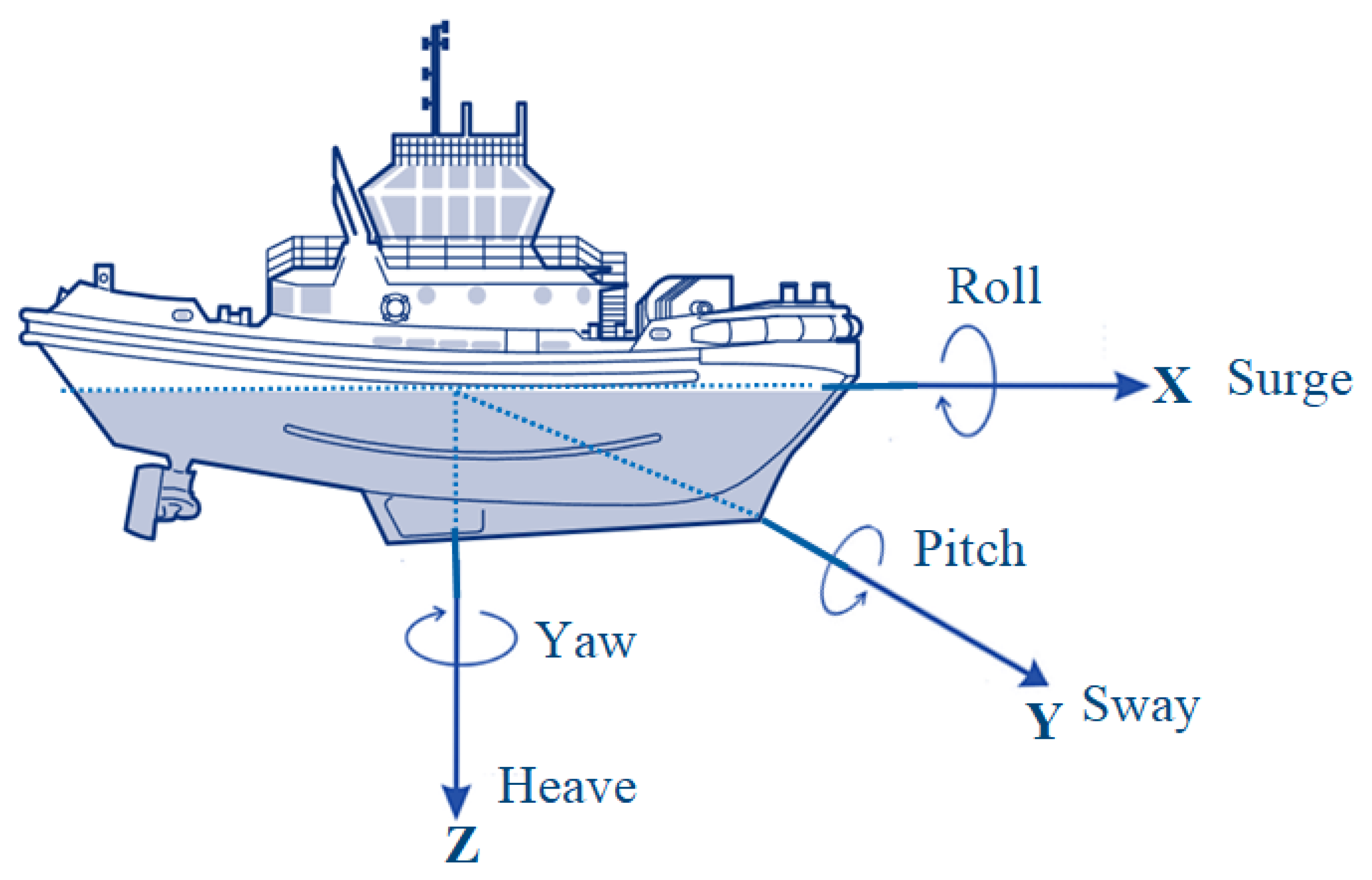
Marine vessels exhibit six degrees of freedom in their motion, encompassing translational movements in the horizontal plane (surge, sway, yaw) and rotational motions (roll, pitch, heave), as illustrated in Figure 2. For the purposes of this study, a one-degrees-of-freedom (1-DOF) ship dynamic model is sufficient to analyze the hybrid renewable energy system (HRES) within the integrated energy and propulsion system framework of marine engineering.

Therefore, the 1 DOF ship dynamic equation governing the forward surge motion of the vessel incorporates external forces and, based on Newton’s second law, can be expressed as follows [50]:

$$\begin{gathered} {\mathrm{M}}_{\mathrm{R}}\ast \dot{{\mathrm{v}}_{\mathrm{s}}}\left(\mathrm{t}\right)={\mathrm{F}}_{\mathrm{h}\mathrm{y}\mathrm{d}}\left(\mathrm{t}\right)-{\mathrm{R}}_{\mathrm{e}\mathrm{n}\mathrm{v}}\left(\mathrm{t}\right)+{\mathrm{F}}_{\mathrm{t}\mathrm{o}\mathrm{w}}\left(\mathrm{t}\right) \\ ⟹{\displaystyle \frac{d{V}_s\left(t\right)}{dt}}={\displaystyle \frac{1}{M_R}}\left[\left(F_{prop}\left(t\right)-R_{resistance}\left(t\right)\right)-R_{env}\left(t\right) \\ \hspace{1em}\hspace{1em}\hspace{1em}\hspace{1em}\hspace{1em}\hspace{1em}\hspace{1em}\hspace{1em}\hspace{1em}+F_{tow}\left(t\right)\right]={\displaystyle \frac{1}{M_R}}\left[F_{prop}\left(t\right)-R_{total}\left(t\right)+F_{tow}\left(t\right)\right] \end{gathered}$$

(1)

where ${\mathrm{M}}_{\mathrm{R}}$ denotes the mass of the rigid body which contains the mass of tugboat and added mass (kg), ${\mathrm{V}}_{\mathrm{s}}\left(\mathrm{t}\right)$ is the surge velocity of the ship or vessel speed (knots or m/s), $\dot{{\mathrm{v}}_{\mathrm{s}}}\left(\mathrm{t}\right)$ is the acceleration of the ship (m/s²), ${\mathrm{F}}_{\mathrm{h}\mathrm{y}\mathrm{d}}\left(\mathrm{t}\right)$ is the hydrodynamic force acting along surge direction (N), and ${\mathrm{R}}_{\mathrm{e}\mathrm{n}\mathrm{v}}\left(\mathrm{t}\right)$ is the environmental forces (N), ${\mathrm{F}}_{\mathrm{p}\mathrm{r}\mathrm{o}\mathrm{p}}\left(\mathrm{t}\right)$ is the propulsive force (N), ${\mathrm{R}}_{\mathrm{r}\mathrm{e}\mathrm{s}\mathrm{i}\mathrm{s}\mathrm{t}\mathrm{a}\mathrm{n}\mathrm{c}\mathrm{e}}\left(\mathrm{t}\right)$ is the resistance force (N), ${\mathrm{R}}_{\mathrm{t}\mathrm{o}\mathrm{t}\mathrm{a}\mathrm{l}}\left(\mathrm{t}\right)$ is the sum of the ${\mathrm{R}}_{\mathrm{e}\mathrm{n}\mathrm{v}}$ and ${\mathrm{R}}_{\mathrm{r}\mathrm{e}\mathrm{s}\mathrm{i}\mathrm{s}\mathrm{t}\mathrm{a}\mathrm{n}\mathrm{c}\mathrm{e}}$(N), ${\mathrm{F}}_{\mathrm{t}\mathrm{o}\mathrm{w}}\left(\mathrm{t}\right)$ is the towing force (N) exerted by tugboat or bollard pull during tug operations (N). In addition, the Section 2.2 elucidates the external forces depicted on the left-hand side of Equation (1).

2.2. Ship Resistances

The hydrodynamic resistance forces (${\mathrm{R}}_{\mathrm{r}\mathrm{e}\mathrm{s}\mathrm{i}\mathrm{s}\mathrm{t}\mathrm{a}\mathrm{n}\mathrm{c}\mathrm{e}})$, which act in opposition to the vessel’s forward motion, encompass various elements: frictional resistance force (${\mathrm{R}}_{\mathrm{f}\mathrm{r}\mathrm{i}\mathrm{c}})$, originating from the drag between the tugboat’s hull surface and the water; and form resistance force (${\mathrm{R}}_{\mathrm{f}\mathrm{o}\mathrm{r}\mathrm{m}})$, which arises from the interaction of the tugboat’s hull shape and profile with the water [51,52]. The equation for the ${\mathrm{R}}_{\mathrm{r}\mathrm{e}\mathrm{s}\mathrm{i}\mathrm{s}\mathrm{t}\mathrm{a}\mathrm{n}\mathrm{c}\mathrm{e}}$ can be expressed as

$$\begin{gathered} R_{resistance}\left(t\right)=R_{fric}\left(t\right)+R_{form}\left(t\right) \\ \hspace{1em}\hspace{1em}\hspace{1em}\hspace{1em}=0.5{ \rho }_w{V_s\left(t\right)}^2 {(C}_f A_{ws}+C_{form }{A}_{cs}) \end{gathered}$$

(2)

where ${\rho }_{\mathrm{w}}$ is the density sea water (kg/m³), ${\mathrm{C}}_{\mathrm{f}}$ is frictional coefficient which ranges from 0.002 to 0.004 (smooth-hulled vessels) and from 0.004 to 0.006 (moderate surface roughness) [52,53], ${\mathrm{A}}_{\mathrm{w}\mathrm{s}}$ is the wetted surface area of the vessel (m²), $C_{form}$ is form resistance coefficient, typical for vessel designed primarily for maneuverability at lower speeds rather than high speed, generally falls within the range of 0.8 to 1.2 [52,53], $A_{cs}$ is the cross-sectional or frontal area of the vessel (m²).

This necessitates that the fully autonomous tugboat must produce adequate towing force to counteract the hydrodynamic resistance of both itself and the towed vessel, ensuring optimal towing performance.

Lastly, the environmental forces (${\mathrm{R}}_{\mathrm{e}\mathrm{n}\mathrm{v}})$, which encompass external forces acting on the vessel from its surrounding natural environment contribute to the total resistance. These forces include random wave forces (${\mathrm{R}}_{\mathrm{w}\mathrm{a}\mathrm{v}\mathrm{e}}$) affecting the hull, current forces (${\mathrm{R}}_{\mathrm{c}\mathrm{u}\mathrm{r}\mathrm{r}\mathrm{e}\mathrm{n}\mathrm{t}}$) influencing the vessel’s hull and appendages due to water currents, and wind forces (${\mathrm{R}}_{\mathrm{w}\mathrm{i}\mathrm{n}\mathrm{d}})$ involving the interaction between the ship and external sea waves, thereby impacting the superstructure components above the waterline [51,52]. The exerted environmental force (${\mathrm{R}}_{\mathrm{e}\mathrm{n}\mathrm{v}}$(t)) is expressed as follows [3,54]:

$$\begin{array}{cc}\hfill R_{env}\left(t\right)& =R_{wave}\left(t\right)+R_{wind}\left(t\right)+R_{current}\left(t\right)\hfill \\ R_{wave}\left(t\right)& ={\displaystyle \frac{1}{2}} {\rho }_{w}g{H\left(t\right)}_{sw}^2 {\left({\displaystyle \frac{2\pi }{T_m\left(t\right)}}\right)}^{2}S\left(f_m\right(t\left)\right)\hfill \\ \hfill R_{wind}\left(t\right)& ={\displaystyle \frac{1}{2}} {\rho }_a{V\left(t\right)}_{rw}^2 C_{wi}{A}_{wi}\hfill \\ & ={\displaystyle \frac{1}{2}} {\rho }_a{\left[V_s\left(t\right)-V_{wi}\left(t\right)cos\left({\beta }_{wi}\right(t)-\psi (t\left)\right)\right]}^2{C}_{wi}{A}_{wi}\hfill \\ \hfill R_{current}\left(t\right)& ={{\displaystyle \frac{1}{2}} \rho }_w {V\left(t\right)}_{c,ship}^2{C_{d,curr}A}_c\hfill \\ & ={{\displaystyle \frac{1}{2}} \rho }_w {\left(V_c\left(t\right)\mathit{cos}\left({\beta }_c\right(t)-\psi (t\left)\right)-V_s\left(t\right)\right)}^2{C_{d,curr}A}_c\hfill \end{array}$$

(3)

where g is the acceleration due to gravity(m/s²), ${\mathrm{H}}_{\mathrm{s}\mathrm{w}}\left(\mathrm{t}\right)$ is the significant wave height (m), ${\mathrm{T}}_{\mathrm{m}}\left(\mathrm{t}\right)$ is the mean wave period between the successive wave crest in a wave train (s), $\mathrm{S}\left({\mathrm{f}}_{\mathrm{m}}\left(\mathrm{t}\right)\right)$ is the spectral density of wave energy at frequency ${\mathrm{f}}_{\mathrm{m}}\left(\mathrm{t}\right)$ in the JONSWAP spectrum [50,55], ${\rho }_{\mathrm{a}}$ is the density of air (kg/m³), ${\mathrm{V}}_{\mathrm{r}\mathrm{w}}\left(\mathrm{t}\right)$ is the velocity of the wind relative to the vessel speed (m/s), ${\mathrm{C}}_{\mathrm{w}\mathrm{i}}$ is the drag coefficient of wind, and ${\mathrm{A}}_{\mathrm{w}\mathrm{i}}$ is the reference area of the tugboat exposed to the wind (m²), ${\mathrm{V}}_{\mathrm{w}\mathrm{i}}\left(\mathrm{t}\right)$ is the wind velocity (m/s), ${\beta }_{\mathrm{w}\mathrm{i}}\left(\mathrm{t}\right)$ is the wind direction (degrees), $\psi \left(\mathrm{t}\right)$ is the ship’s course (degrees), ${\mathrm{V}}_{\mathrm{c},\mathrm{s}\mathrm{h}\mathrm{i}\mathrm{p}}\left(\mathrm{t}\right)$ is the velocity of sea or water current relative to the vessel (m/s), $C_{d,curr}$ is the drag coefficient of the vessel with respect to currents, ${\mathrm{A}}_{\mathrm{c}}$ is the reference or cross section area of the tugboat exposed to the current force (m²), ${\mathrm{V}}_{\mathrm{c}}\left(\mathrm{t}\right)$ is the current velocity along x-axis (m/s), and ${\beta }_{\mathrm{c}}\left(\mathrm{t}\right)$ is the sea current direction (degrees).

2.3. Modeling of Propeller

The propeller hydrodynamic forces (${\mathrm{F}}_{\mathrm{p}\mathrm{r}\mathrm{o}\mathrm{p}})$ produced by the propeller’s interaction with the water contributes to the propulsive force. The propeller hydrodynamic forces can be expressed as [56,57]:

$$F_{prop}\left(t\right)=T_{prop}\left(t\right)\left(1-T_{dc}\right)\ast N_{prop}\left(t\right)$$

(4)

where ${\mathrm{T}}_{\mathrm{p}\mathrm{r}\mathrm{o}\mathrm{p}}\left(\mathrm{t}\right)$ denotes the propeller thrust (N), ${\mathrm{N}}_{\mathrm{p}\mathrm{r}\mathrm{o}\mathrm{p}}\left(\mathrm{t}\right)$ denotes the number of propellers (unitless), and ${\mathrm{T}}_{\mathrm{d}\mathrm{c}}$ is the thrust deduction coefficient (unitless) which is estimated using empirical relation, and this is expressed as follows [58]:

$$T_{dc}=0.21593+0.099768\ast C_b-{\displaystyle \frac{D_{prop}}{\sqrt{B_{ship}\ast d_{ship}}}}$$

(5)

where ${\mathrm{C}}_{\mathrm{b}}$ is the block coefficient, which is approximately 0.53 [59], ${\mathrm{D}}_{\mathrm{p}\mathrm{r}\mathrm{o}\mathrm{p}}$ is the propeller diameter (m), $B_{ship}$ is the breadth of the ship (m), and $d_{ship}$ denotes the draft of the ship (m). For ships equipped with a single propeller, the $T_{dc}$ typically ranges from 0.12 to 0.30 [60].

The propeller component takes as input the rotational speed of the propeller ($n_{prop}\left(t\right)$) and the ship’s speed (${\mathrm{V}}_{\mathrm{s}}\left(\mathrm{t}\right)$), which are provided by the engine shaft and ship components, respectively. Thus, the propeller inflow velocity in the presence of wake ${\mathrm{V}}_{\mathrm{w}\mathrm{p}}\left(\mathrm{t}\right)$ and propeller inflow velocity without interference ${\mathrm{V}}_{\mathrm{h}\mathrm{y}}\left(\mathrm{t}\right)$ are expressed as

$$\begin{gathered} V_{wp}\left(t\right)=V_s\left(t\right)[1-\omega \left(t\right)]] \\ {V}_{hy}\left(t\right)=\sqrt{{V_{wp}\left(t\right)}^2+{\left(0.7\pi D_{prop}{n}_{prop}\right(t\left)\right)}^2} \end{gathered}$$

(6)

where $\omega \left(\mathrm{t}\right)$ is the wake fraction coefficient (unitless), which can be determined from an empirical formula based on Taylor’s model as $\omega \left(\mathrm{t}\right)=-0.05+0.5\ast C_b$. However, for ships equipped with a single propeller, the $\omega \left(\mathrm{t}\right)$ typically ranges from 0.20 to 0.45 [60,61].

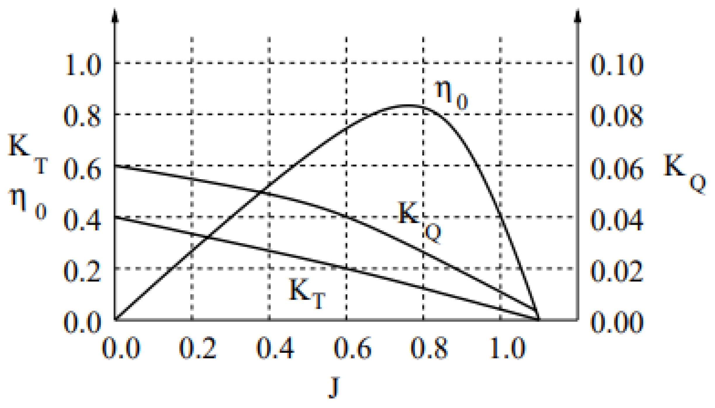
The output of the propeller includes the torque (${\mathrm{T}}_{\mathrm{p}\mathrm{r}\mathrm{o}\mathrm{p}}\left(\mathrm{t}\right)$), which is transmitted to the engine shaft component, and the propeller thrust (${\mathrm{Q}}_{\mathrm{p}\mathrm{r}\mathrm{o}\mathrm{p}}\left(\mathrm{t}\right)$), which is delivered to the ship component. The propeller thrust and torque when considering open water can be expressed as [56,57]:

$$\begin{gathered} T_{prop}\left(t\right)=K_T{\left(J\right)\rho }_w{D_{prop}}^4{n_{prop}\left(t\right)}^2 \\ {Q}_{prop}\left(t\right)=K_Q{\left(J\right)\rho }_w{D_{prop}}^5{n_{prop}\left(t\right)}^2 \\ {K}_T\left(J\right)={\beta }_1-{\beta }_{2}J\left(t\right) \\ {K}_Q\left(J\right)={\gamma }_1-{\gamma }_{2}J\left(t\right) \\ J\left(t\right)={\displaystyle \frac{V_{wp}\left(t\right)}{n_{prop}\left(t\right)D_{prop}}}={\displaystyle \frac{V_s\left(t\right)[1-\omega \left(t\right)]]}{n_{prop}\left(t\right)D_{prop}}} \\ {\eta }_o\left(t\right)={\displaystyle \frac{J\left(t\right)K_T\left(J\right)}{2\pi K_Q\left(J\right)}} \end{gathered}$$

(7)

where ${\mathrm{K}}_{\mathrm{T}}\left(J\right)$ is thrust coefficient, J(t) is the advance coefficient,${\rho }_{\mathrm{w}}$ is the density of sea or water (kg/m³) ${\mathrm{D}}_{\mathrm{p}\mathrm{r}\mathrm{o}\mathrm{p}}$ is the propeller diameter (m), ${\mathrm{K}}_{\mathrm{Q}}\left(J\right)$ is the torque coefficient, ${\mathrm{V}}_{\mathrm{w}\mathrm{p}}\left(\mathrm{t}\right)$ is the water speed at the propeller or speed of advance (m/s), $\omega \left(\mathrm{t}\right)$ is the wake fraction, and $n_{prop}$ is the propeller rotational velocity (rad/s), and ${\eta }_{\mathrm{o}}\left(\mathrm{t}\right)$ is the open-water propeller efficiency. The four coefficients (${\beta }_1,{\beta }_1,{\gamma }_1,{\gamma }_2)$ for the propeller thrust and torque are illustrated in Figure 3, and likewise, the power consumed by the propeller, ${\mathrm{P}}_{\mathrm{p}\mathrm{r}\mathrm{o}\mathrm{p}}\left(\mathrm{t}\right),$ is given by ${\displaystyle \frac{{2\pi n}_{prop}\left(t\right)Q_{prop}\left(t\right)}{{\eta }_o\left(t\right)}}$.

2.4. Modeling of Gearbox

The gearbox, which is connected between the motor and propeller, optimizes the power transmission from the motor to the propeller by balancing both the torque and rotational speed for effective and efficient ship movement at a certain gearbox reduction ratio ${\lambda }_{gear}$. The equation of gearbox in relation to the motor and propulsion torque is expressed as follows:

$$\begin{gathered} Q_{motor}\left(t\right)={\displaystyle \frac{Q_{prop}\left(t\right)}{\left(\frac{{\eta }_{gear }}{{\lambda }_{gear}}\right)}}=Q_{prop}\left(t\right)\ast \left({\displaystyle \frac{{\eta }_{gear }}{{\lambda }_{gear}}}\right) \\ {\omega }_{motor}\left(t\right)=2\ast \pi \ast {\lambda }_{gear}\ast n_{prop}\left(t\right) \end{gathered}$$

(8)

where ${\mathrm{Q}}_{\mathrm{m}\mathrm{o}\mathrm{t}\mathrm{o}\mathrm{r}}\left(\mathrm{t}\right)$ is the motor torque (Nm), ${\eta }_{gear}$ denotes the gear efficiency, and ${\omega }_{motor}\left(\mathrm{t}\right)$ is the angular velocity of the motor (rad/s). Furthermore, the gearbox, propeller shaft, and propeller are subjected to the load-side torque (or resistance torque) $Q_{load}\left(t\right)$, which must be overcome by the engine to propel the ship. The governing equations for the propulsion system’s shafting components are given as follows [44]:

$$\begin{gathered} Q_{load}\left(t\right)={\displaystyle \frac{Q_{prop,act}\left(t\right)}{{\lambda }_{gear} {\eta }_{shaft}}} \\ {Q}_{prop,act}\left(t\right)={\displaystyle \frac{Q_{prop}\left(t\right)}{{\eta }_{\mathrm{R}}}} \\ {\omega }_{engine}\left(t\right)={\lambda }_{gear}\ast {\omega }_{\mathrm{p}\mathrm{r}\mathrm{o}\mathrm{p}}\left(\mathrm{t}\right) \end{gathered}$$

(9)

where $Q_{prop,act}\left(t\right)$ is the actual propeller torque, ${\eta }_{shaft}$ is the mechanical efficiency of the shaft, ${\eta }_{\mathrm{R}}$ is the relative rotative efficiency (on ships with a single propeller it typically ranges from 1.0 to 1.07, while for two propellers it is approximately 0.98 [60]), and ${\omega }_{\mathrm{e}\mathrm{n}\mathrm{g}\mathrm{i}\mathrm{n}\mathrm{e}}\left(\mathrm{t}\right)$ and ${\omega }_{\mathrm{p}\mathrm{r}\mathrm{o}\mathrm{p}}\left(\mathrm{t}\right)$, are the angular velocities of the engine and propeller (rad/s) respectively.

2.5. Modeling of Motor

The motor forms the core of the propulsion system in converting energy into mechanical power to drive the propeller shaft. The motor is modeled in relation to the engine’s angular velocity using the simple Willian’s equation as follows:

$$\begin{gathered} {\omega }_{engine}\left(t\right)\ast Q_{motor}\left(t\right)=e\ast P_{motor}\left(t\right)-P_0 \\ {Q}_{motor}\left(t\right)={\mathrm{f}}_{\mathrm{m}\mathrm{o}\mathrm{t}\mathrm{o}\mathrm{r}}\ast {\mathrm{C}}_{\mathrm{m}\mathrm{o}\mathrm{t}\mathrm{o}\mathrm{r}} \end{gathered}$$

(10)

where $P_{motor}\left(t\right)$ is the motor electrical power (kW), the coefficients e and $P_0$ are the Willan’s constants associated with power conversion efficiency and valued at 0.9598 kW/Nm and 358.18 kW, respectively [44], $C_{motor}$ is the torque command as a percentage of the maximum torque fed to the drive or torque distribution ratio of the motor, and $f_{motor}$ is the unit conversion factor or torque coefficient constant for the motor.

2.6. Rotational Dynamic Interaction with Propeller, Motor, and Engine

During tugboat operations, the hull, propeller, and engine interact along the surge direction. Also, the wave-induced forces drive the hull’s surge motion, impacting the propeller’s efficiency and thrust, while the engine adjusts its power output to compensate. This rotational dynamic interaction, essential for maintaining consistent propulsion and stability in a fluctuating wave environment, is modeled using the following equation:

$$J_{total}{\displaystyle \frac{d{\omega }_{engine}\left(t\right)}{dt}}=Q_{engine}\left(t\right)+Q_{motor}\left(t\right)-Q_{load}\left(t\right)$$

(11)

where ${\mathrm{J}}_{\mathrm{t}\mathrm{o}\mathrm{t}\mathrm{a}\mathrm{l}}$ is the total moment of inertia of the system, which consists of the moment of the propeller, gear, added mass, engine, motor, and propeller shaft (kg·m²), ${\displaystyle \frac{\mathrm{d}{\omega }_{engine}\left(t\right)}{\mathrm{d}\mathrm{t}}}$ is the engine angular acceleration (rad/s²), and ${\mathrm{Q}}_{\mathrm{e}\mathrm{n}\mathrm{g}\mathrm{i}\mathrm{n}\mathrm{e}}\left(\mathrm{t}\right)$ is the engine delivered torque at the shaft or engine brake torque output (Nm).

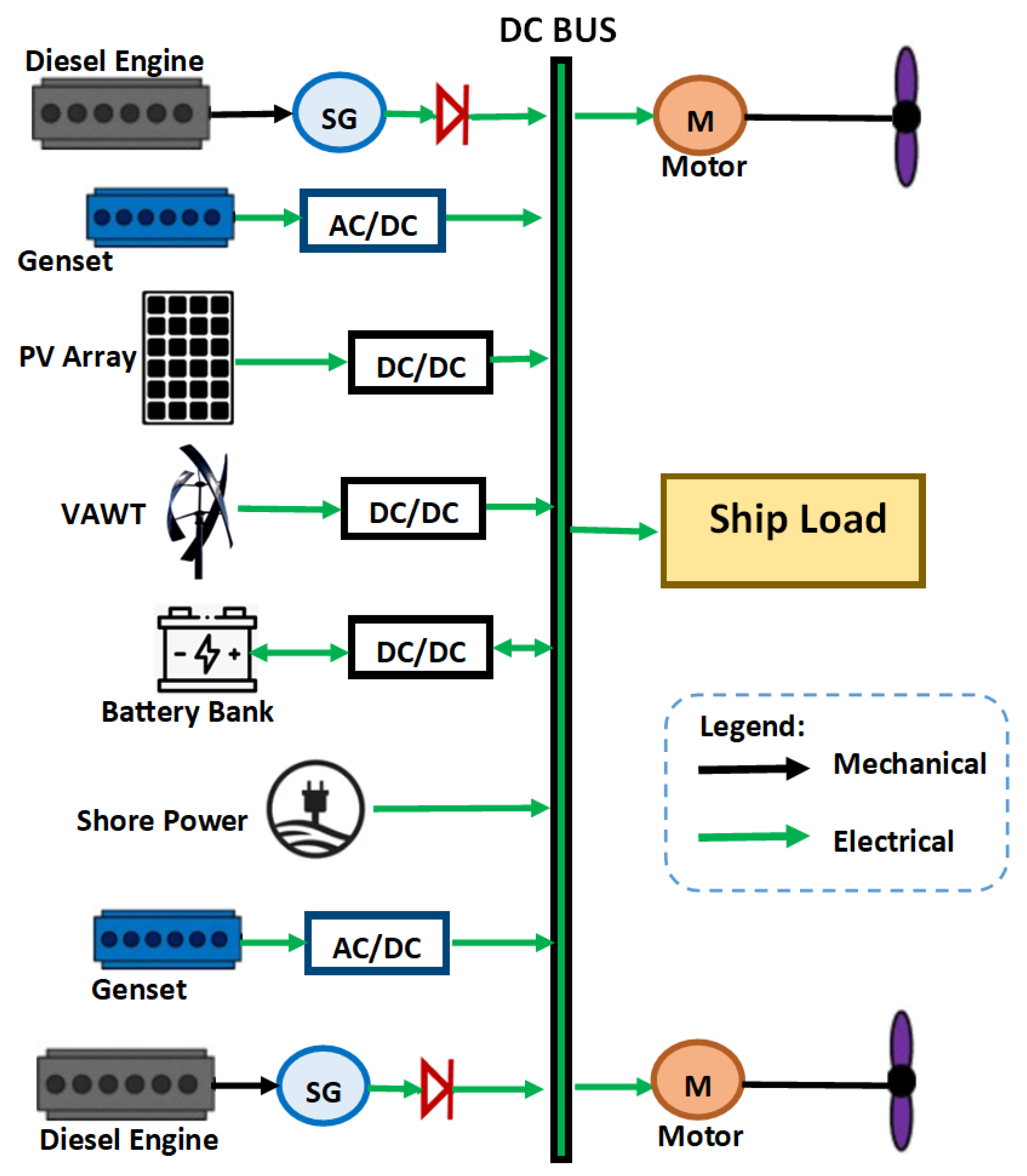
2.7. Modeling of the Power Distribution System

The power distribution system is illustrated in Figure 4. On the DC bus’s left side, power generation components include two diesel engines, two synchronous generators (SGs), additional diesel generators (Gensets), photovoltaic (PV) arrays, two vertical axis wind turbines (VAWTs), a battery bank, and shore power. On the right side of the DC bus, the energy consumption includes the propulsion system (motor, propeller shaft, thrusters, and propeller) and the ship’s electrical loads (auxiliary systems and hotel services). To ensure optimal efficiency of the vessel, the fully autonomous tugboat dynamically alternates between renewable energy sources, the battery bank, and Gensets to supply the ship load, while the propulsion load demands are fulfilled by the marine diesel engines and the battery bank. Additionally, the battery bank is recharged through the utilization of the Gensets and surplus green energy.

Furthermore, the SGs are connected to rectifiers for AC/DC conversion to the DC link, while diesel generators use AC/DC converters to stabilize the DC output. In addition, the PV arrays and VAWTs connect to dedicated DC/DC converters for efficient power delivery. Similarly, the battery bank employs a bidirectional converter for charging, discharging, shore power connection, and to support the integration with renewable energy sources. The DC power distribution system, or the DC hub, is preferred for its stability, reduced weight of components, cost-effectiveness, and environmental benefits compared to AC systems [62,63,64]. This paper focuses on the primary power generation sources and energy consumption within the power generation system, omitting other electrical connectors.

2.7.1. Diesel Engine Model

The diesel engine acts as the primary source of mechanical power for propulsion. The rotational motion produced by the diesel engine is transferred to the propeller shaft, which then drives the propeller, enabling the vessel to move through the water. The diesel engine model is derived based on the engine’s operating points along the lug curve and its power rating from the technical operating profile. Therefore, the mechanical output power of the engine ${\mathrm{P}}_{\mathrm{e}\mathrm{n}\mathrm{g}\mathrm{i}\mathrm{n}\mathrm{e}}\left(\mathrm{t}\right)$ in conjunction with engine torque can be expressed as follows:

$$\begin{gathered} P_{engine,mech}\left(t\right)={s_{engine}\left(t\right)\ast N}_{engine}\left(t\right)\ast Q_{engine}\left(t\right)\ast {\omega }_{engine}\left(t\right) \\ {Q}_{engine}\left(t\right)=C_1\ast C_{engine}+C_2\ast {RPM}_{engine}^2+C_3\ast {RPM}_{engine}+C_4 \end{gathered}$$

(12)

where $s_{engine}\left(\mathrm{t}\right)$ is the binary number for engine switch status using 1 (ON) and 0 (OFF), and ${\mathrm{N}}_{\mathrm{e}\mathrm{n}\mathrm{g}\mathrm{i}\mathrm{n}\mathrm{e}}$ is the number of engines in operation(unitless), ${\mathrm{R}\mathrm{P}\mathrm{M}}_{\mathrm{e}\mathrm{n}\mathrm{g}\mathrm{i}\mathrm{n}\mathrm{e}}$ is the engine rotational shaft speed (rpm), which equals ${\displaystyle \frac{{60\ast \omega }_{engine}\left(t\right)}{2\pi }}$, $C_{engine}$ is the engine torque command (%), and ${\mathrm{C}}_1$, ${\mathrm{C}}_2$, ${\mathrm{C}}_3$, and ${\mathrm{C}}_4$ are the coefficients determined from a dynamometer test or engine simulation.

Likewise, the quadratic relation between the diesel engine mass flow rate of the total fuel consumption ${\dot{\mathrm{m}}}_{\mathrm{e}\mathrm{n}\mathrm{g}\mathrm{i}\mathrm{n}\mathrm{e}}$ (kg/min) and the mechanical power output under variable speed operations can be approximated as follows:

$${\dot{m}}_{engine} \left(t\right)=4\ast {10}^{-4}{P}_{engine}^2\left(t\right)-0.3502P_{engine}\left(t\right)+111.92$$

(13)

In addition, the synchronous generator transforms mechanical energy derived from the diesel engine into electrical energy. The interconnection between the generator and the diesel engine occurs via the propeller shaft, where the torque produced by the diesel engine $Q_{engine}\left(t\right)$ serves as an input to the synchronous generator. Therefore, electrical output power for engine ${\mathrm{P}}_{\mathrm{e}\mathrm{n}\mathrm{g}\mathrm{i}\mathrm{n}\mathrm{e},\mathrm{m}\mathrm{e}\mathrm{c}\mathrm{h}}\left(\mathrm{t}\right)$ and synchronous generator efficiency ${\eta }_{SG}\left(t\right)$ based on empirical data are expressed as follows:

$$P_{engine,elec}\left(t\right)=P_{engine,mech}\left(t\right)\ast {\eta }_{SG}\left(t\right)$$

(14)

2.7.2. Marine Diesel Generator Model

The marine diesel generator (or Genset) is used to supply the ship’s onboard electrical load. In addition, the Genest is used to charge batteries and provide power as an emergency back up during power failures. The total diesel Genest output power ${\mathrm{P}}_{\mathrm{g}\mathrm{e}\mathrm{n}\mathrm{s}\mathrm{e}\mathrm{t}}\left(\mathrm{t}\right)$ [12] can be expressed as follows:

$$P_{genset,mech}\left(t\right)=P_{genset,nom}\ast {\eta }_{brake}\ast N_{Genset}\ast {\eta }_{genset}$$

(15)

where $P_{genset,\mathrm{n}\mathrm{o}\mathrm{m}}$ denotes the nominal power (kW), ${\eta }_{brake}$ is the brake thermal efficiency, while ${\mathrm{N}}_{\mathrm{G}\mathrm{e}\mathrm{n}\mathrm{s}\mathrm{e}\mathrm{t}}$ and ${\eta }_{\mathrm{g}\mathrm{e}\mathrm{n}\mathrm{s}\mathrm{e}\mathrm{t}}$ are number of Gensets(unitless), and Gensets efficiency (%). In addition, the mass flow rate of the total fuel consumption ${\dot{\mathrm{m}}}_{\mathrm{G}\mathrm{e}\mathrm{n}\mathrm{s}\mathrm{e}\mathrm{t}}$ is determined using the linear least-squares method, ensuring optimal alignment with the Gensets data by minimizing the overall deviation between the observed and predicted values. This approach guarantees accurate fuel consumption predictions across a range of Genset power outputs. The equation to determine the ${\dot{m}}_{genset}\left(t\right)$, (kg/min) is as follows:

$${\dot{m}}_{genset}\left(t\right)=0.005 P_{genset,mech}\left(t\right)+0.1095$$

(16)

2.7.3. Photovoltaic Modules (PV) Model

The photovoltaic modules are to be installed on the starboard and port sides of the vessel. The daily solar energy output from the PV cells under standard testing conditions (STC) is described as follows [12]:

$$\begin{gathered} P_{PV}\left(t\right)=P_{PV,nom}\ast {N_{PV,modules}\ast {\eta }_{wire,eff}\ast \eta }_{PV-cell,eff}\ast {\displaystyle \frac{I_{amb}\left(t\right)}{I_{STC}}} \\ \ast \left[1-{\lambda }_{PV,temp}\ast \left\{T_{amb}\left(t\right)+I_{amb}\left(t\right)\ast \left({\displaystyle \frac{NOCT-20}{I_{PV,cell}}}\right)-T_{PV,STC} \right\}\right] \end{gathered}$$

(17)

where $P_{PV}\left(t\right)$ is the total power generated by the PV panels at time t (kWh), ${\mathrm{P}}_{\mathrm{P}\mathrm{V},\mathrm{n}\mathrm{o}\mathrm{m}}$ is the nominal or rating power of the PV cells (kW), $N_{PV,modules}$ is the number of PV panels (unitless), ${\eta }_{\mathrm{P}\mathrm{V}-\mathrm{c}\mathrm{e}\mathrm{l}\mathrm{l},\mathrm{e}\mathrm{f}\mathrm{f}}$ is the efficiency of the PV panel (%), ${\eta }_{\mathrm{w}\mathrm{i}\mathrm{r}\mathrm{e},\mathrm{e}\mathrm{f}\mathrm{f}}$ denotes the efficiency of the wire (%), ${\mathrm{I}}_{\mathrm{a}\mathrm{m}\mathrm{b}}\left(\mathrm{t}\right)$ is the ambient radiation intensity at time t (kW/m²), ${\mathrm{I}}_{\mathrm{S}\mathrm{T}\mathrm{C}}$ is the radiation intensity at the standard test conditions (1 kW/m²), ${\lambda }_{PV,temp}$ is the temperature coefficient of the PV modules (%/°C), $T_{amb}$ is the ambient temperature at the study area (°C), $NOCT$ is the nominal operating cell temperature (°C), $I_{PV,cell}$ is the radiation intensity on cell surface (0.8 kW/m²), and $T_{PV,STC}$ is the PV cell nominal temperature at the standard test conditions (25 °C).

2.7.4. Vertical Axis Wind Turbines (VAWT) Model

Vertical Axis Wind Turbines (VAWTs) are selected for this study due to their quieter operation, ease of maintenance, capability to generate power at low cut-in speeds, and suitability for close clustering. Energy output is influenced by the VAWTs hub height, local wind speed, and ship speed. This research proposes the installation of two VAWTs: one on the starboard mast and the other on the port mast. Each VAWT is fitted with a permanent magnet synchronous generator that converts the mechanical energy from the rotating blades into electrical power. Using the wind power law profile, the VAWT speed at the turbine height $V_{VAWT,hub}$ can be expressed as [12]:

$$V_{VAWT,hub}=V_{anemo}\ast {\left[{\displaystyle \frac{H_{VAWT,hub}}{H_{anemo}}}\right]}^{\alpha }$$

(18)

where ${\mathrm{V}}_{\mathrm{a}\mathrm{n}\mathrm{e}\mathrm{m}\mathrm{o}}$ is the wind speed at the anemometer height (m/s), ${\mathrm{H}}_{\mathrm{V}\mathrm{A}\mathrm{W}\mathrm{T},\mathrm{h}\mathrm{u}\mathrm{b}}$ is the hub height of the VAWT above waterline (m), ${\mathrm{H}}_{\mathrm{a}\mathrm{n}\mathrm{e}\mathrm{m}\mathrm{o}}$ is the height of the anemometer (m), and $\mathsf{\alpha }$ power law exponent for the United State of America equal to 0.216 [65].

Given that the tugboat is in motion, the relative speed $V_{rel}\left(t\right)$ is determined by the wind speed at the hub, $V_{wi}\left(t\right)$, ship speed $V_s\left(t\right)$, wind direction ${\beta }_{wi}\left(t\right)$, and ship heading $\phi \left(t\right).$ This relationship is illustrated in Figure 5, and it can be expressed as follows:

$$V_{rel}\left(t\right)={\left\{\begin{array}{c}{V_s\left(t\right)}^2+{V_{VAWT,hub}\left(t\right)}^2-2V_s\left(t\right)\\ \ast V_{VAWT,hub}\left(t\right)cos(\phi \left(t\right)-{\beta }_{wi}\left(t\right))\end{array}\right\}}^{0.5}$$

(19)

Similarly, the output mechanical power extracted from the wind by the VAWT $P_{VAWT,mech}\left(t\right)$ can be modeled using the three distinct regions based on wind speed, and these are expressed as follows:

$$\begin{gathered} \begin{array}{l}{P}_{VAWT,mech}\left(t\right)\\ =\left\{\begin{array}{c}{\displaystyle \frac{1}{2}}{\rho }_a A_{VAWT} C_{p,VAWT}\left(\lambda ,\beta \right)\ast {V_{rel}\left(t\right)}^3 V_{ci}<V_{rel}\left(t\right)<V_r\\ P_{VAWT,nom} V_r<V_{rel}\left(t\right)<V_{co}\\ 0 V_{rel}\left(t\right)<V_{ci} or V_{rel}\left(t\right)<V_{co}\end{array}\right\} \\ \lambda ={\displaystyle \frac{R_{VAWT}\ast {\omega }_{VAWT}}{V_{rel}\left(t\right)}}\end{array} \end{gathered}$$

(20)

where $V_{ci}$ is the VAWT cut-in wind speed (m/s), $V_{co}$ is the VAWT cut-off speed (m/s), V_r is the rated wind speed for VAWT (m/s), ${\mathrm{A}}_{\mathrm{V}\mathrm{A}\mathrm{W}\mathrm{T}}$ is the swept area of the wind turbine (m²), ${\mathrm{C}}_{\mathrm{p},\mathrm{V}\mathrm{A}\mathrm{W}\mathrm{T}}\left(\lambda ,\beta \right)$ is the power coefficient, which is function of tip speed $\lambda$ and the pitch angle $\beta$ of the VAWT, ${\mathrm{R}}_{\mathrm{V}\mathrm{A}\mathrm{W}\mathrm{T}}$ is the radius of turbine blade (m), ${\omega }_{VAWT}$ is the VAWT rotor speed (rad/s), and $P_{VAWT,nom}$ is the nominal power of the VAWT. In addition, $C_{p,VAWT}\left(\lambda ,\beta \right)$ can be expressed as the mechanical parameters of the VAWT model as follows [66]:

$$\begin{gathered} C_{p,VAWT}\left(\lambda ,\beta \right)=0.5\left({\displaystyle \frac{116}{\xi }}-0.4\beta -5\right)exp\left({\displaystyle \frac{-16.5}{\xi }}\right)+0.006\lambda \\ \xi ={\left({\displaystyle \frac{1}{0.089\beta +\lambda }}-{\displaystyle \frac{0.035}{1+{\beta }^3}}\right)}^{-1} \end{gathered}$$

(21)

Furthermore, the output electrical power VAWT ${\mathrm{P}}_{\mathrm{V}\mathrm{A}\mathrm{W}\mathrm{T},\mathrm{e}\mathrm{l}\mathrm{e}\mathrm{c}}\left(\mathrm{t}\right)$ based on Equation (21) can be expressed as follows:

$$P_{VAWT,elec}\left(t\right)=P_{VAWT,mech}\left(t\right)\ast N_{VAWT}\ast {\eta }_{total,VAWT}$$

(22)

where $N_{VAWT}$ is the number of VAWTs (unitless), and ${\eta }_{\mathrm{t}\mathrm{o}\mathrm{t}\mathrm{a}\mathrm{l},\mathrm{V}\mathrm{A}\mathrm{W}\mathrm{T}}$ denotes the overall efficiency of the VAWT, which consists of the losses in mechanical conversion and electrical generation [%].

2.7.5. Battery Model

The battery bank stores excess energy from the prime mover, Gensets, and/or renewable sources during low-demand periods. This research favors lithium-ion (Li-ion) batteries over lead-acid, nickel-metal-hydride, silver-zinc, and open water-powered batteries due to their superior chemistry [12]. When the combined power from the renewable energy sources and Gensets exceeds the load or when the state of charge SOC(t) is less than the minimum ${ SOC}_{min}\left(t\right)$ the battery bank is charged. The charging power of the battery bank is determined by

$$\begin{gathered} P_{battery}\left(t\right)=P_{battery}\left(t-1\right)\ast \left(1-\sigma \right)+\left[ \sum P_i\left(t\right)-{\displaystyle \frac{P_{ load \left(t\right)}}{{\eta }_{inveter} }}\right] \\ \ast {\eta }_{batt,ch} \end{gathered}$$

(23)

Conversely, when load demand surpasses the available generated energy or when the SOC(t) is greater than maximum ${ SOC}_{max}\left(t\right)$, the battery bank discharges. The available capacity of the battery bank during discharge is determined as follows:

$$\begin{gathered} P_{battery}\left(t\right)=P_{battery}\left(t-1\right)\ast \left(1-\sigma \right)-\left[-\sum P_i\left(t\right)+{\displaystyle \frac{P_{ load \left(t\right)}}{{\eta }_{inveter} }}\right] \\ \ast { \eta }_{batt,disch} \end{gathered}$$

(24)

where ${\mathrm{P}}_{\mathrm{b}\mathrm{a}\mathrm{t}\mathrm{t}\mathrm{e}\mathrm{r}\mathrm{y}}\left(\mathrm{t}\right)$ is the available battery bank power during charging and discharging at time t, ${\mathrm{P}}_{\mathrm{b}\mathrm{a}\mathrm{t}\mathrm{t}\mathrm{e}\mathrm{r}\mathrm{y}}\left(\mathrm{t}-1\right)$ is the available battery bank power at time (t − 1), $\mathsf{\sigma }$ is the self-discharge rate of the battery bank, ${\mathrm{P}}_i\left(t\right)$ is the total power generated by the PVs, VAWTs, Gensets (kW), ${\eta }_{inveter}$ is the AC-DC inverter efficiency, ${\eta }_{batt,ch}$ is battery efficiency during charging process, and ${\eta }_{batt,disch}$ 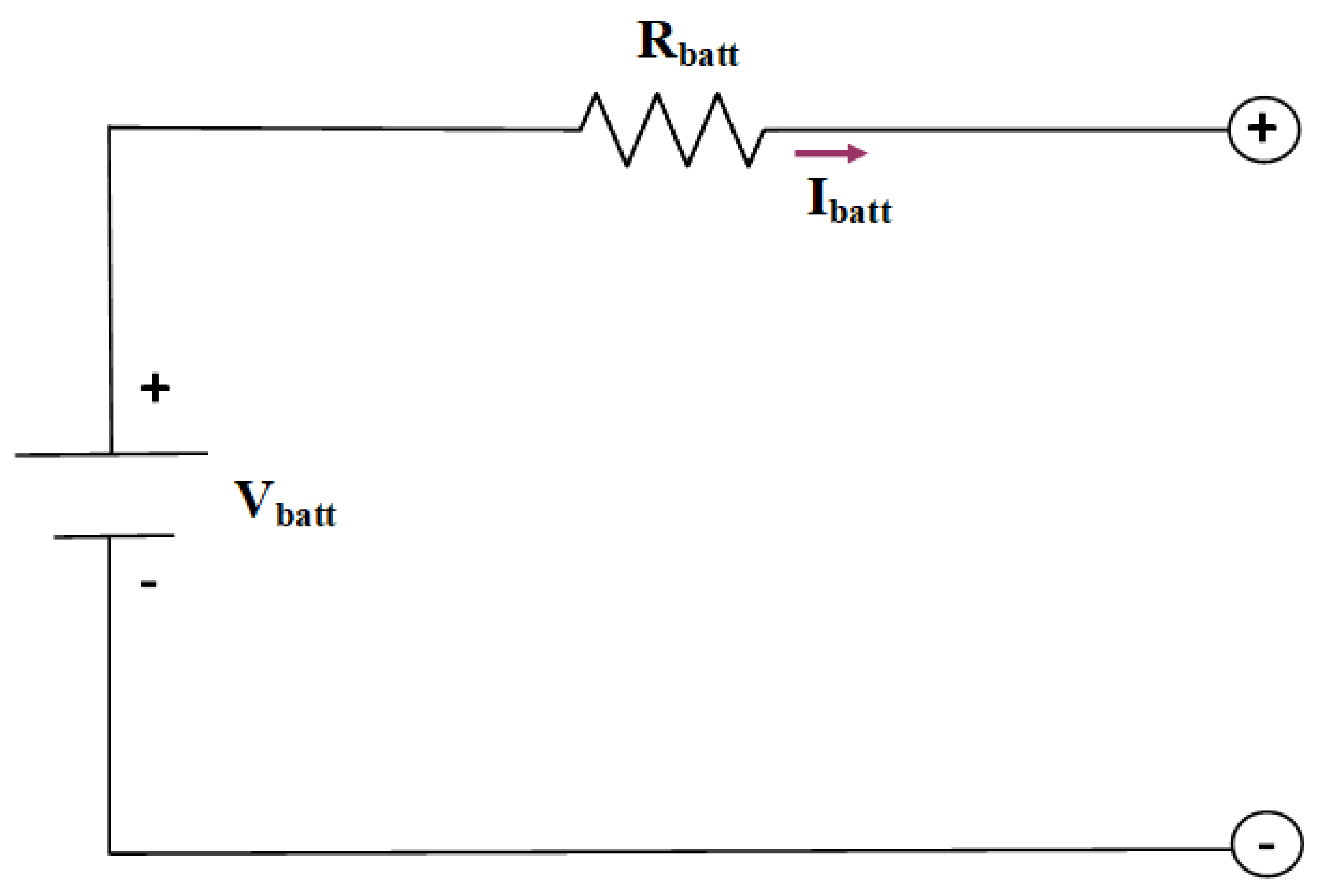is battery efficiency during discharging process. In addition, using the battery model known as internal resistance model or Rint model is shown in Figure 6, and the battery SOC and battery current (${\mathrm{I}}_{\mathrm{b}\mathrm{a}\mathrm{t}\mathrm{t}})$ can be expressed as follows:

$$\begin{gathered} {\displaystyle \frac{d SOC}{dt}}={\displaystyle \frac{I_{batt}\ast {\eta }_{colm}}{3600 Q}} \\ {I}_{batt}={\displaystyle \frac{V_{batt}-\sqrt{V_{batt}-4P_{battery}{R}_{batt}}}{2R_{batt}}} \end{gathered}$$

(25)

where Q denotes the battery capacity (Ah), ${\eta }_{\mathrm{c}\mathrm{o}\mathrm{l}\mathrm{m}}$ is the coulombic efficiency (%), $V_{batt}$ is the battery open-circuit voltage (V), and $R_{batt}$ is the battery resistance (ohms).

2.7.6. Environmental Assessment

Tugboats are known to produce high emissions due to their speed and diverse operational modes. Specifically, the mass emission rate (MER) measures the pollutants emitted from the combustion of fuel in the main engines and Gensets. Thus, the key pollutants include carbon monoxide (CO), carbon dioxide (CO₂), sulfur oxides (SO_x), nitrogen oxides (NO_x), nitrous oxide (N₂O), particulate matter (PM), and unburned hydrocarbons (UHC) or methane (CH₄). The MER is expressed as follows [67]:

$$\begin{gathered} {{MER}_{total}\left(t\right)=MER}_{engine}\left(t\right)+{MER}_{genset}\left(t\right) \\ =\sum _{n=1}^{n=N}{EF}_j\ast \left[{\dot{m}}_{engine}\left(t\right)+{\dot{m}}_{genset}\left(t\right)\right]=\sum _{n=1}^{n=N}{EF}_j\ast \left[ {\dot{m}}_{total}\left(t\right)\right] \end{gathered}$$

(26)

where ${\mathrm{M}\mathrm{E}\mathrm{R}}_{\mathrm{t}\mathrm{o}\mathrm{t}\mathrm{a}\mathrm{l}}\left(\mathrm{t}\right)$ is the total mass emission rate (kg/h), ${\dot{m}}_{total}\left(t\right)$ denotes the total mass flow rate of fuel consumption from both the diesel engines and Genset (kg/h), ${EF}_j$ denotes the emission factor for each pollutant (g/kg-fuel), and j is the type of pollutant for marine fuel (unitless). Furthermore, for new vessels, including fully autonomous tugboats, the IMO requires the implementation of energy efficiency measures, represented by the energy efficiency operational indicator (EEOI) [68], to ensure regulatory compliance. However, the application of EEOI in tugboats may differ due to their unique operational patterns, such as frequent short trips and fluctuating loads. Consequently, reducing fuel consumption throughout the voyage is an effective approach to lowering the EEOI (kg/ton-nm), is expressed as follows:

$$EEOI={\displaystyle \frac{\sum _j{EF}_{{CO}_2,j}\ast \left[m_{total}\left(t\right)\right]}{m_{cargo}\ast D}}$$

(27)

where ${EF}_{{CO}_2,j}$ denotes the emission factor for the CO₂ for the fuel type j, ${\mathrm{m}}_{\mathrm{t}\mathrm{o}\mathrm{t}\mathrm{a}\mathrm{l}}\left(\mathrm{t}\right)$ is the total fuel consumption (kg), $m_{cargo}$ signifies the weight of the cargo in metric tons (or number of passengers), and D is the distance in nautical miles corresponding to the cargo carried or work done.

Furthermore, the emission cost or penalty (EC), which considered a cost factor in the HRES assessment, reflects the environmental cost of using non-renewable energy sources compared to renewable alternatives. Its purpose is to create an economic incentive for reducing emissions [69,70]. The EP is expressed as follows [67]:

$$EC=\sum _{n=1}^{n=N}{C}_j\ast \left[{\dot{m}}_{engine}\left(t\right)+{\dot{m}}_{genset}\left(t\right)\right]$$

(28)

where ${\mathrm{C}}_{\mathrm{j}}$ denotes the environmental cost of emission (USD/kg).

2.8. Estimation of Propeller Load

Understanding propeller load disturbances is essential for maintaining system equilibrium and solving the optimal HRES management problem. The effect of random waves on propeller torque is validated through extended Kalman filtering (EKF). Propeller torque can be estimated using an extended state observer (ESO) with engine speed and torque measurement [32]. Therefore, the accurate estimation of this influence is crucial for optimal HRES management and torque data. Additionally, based on propeller strip theory, propeller rotation power (${\mathrm{P}}_{\mathrm{p}\mathrm{r}\mathrm{o}\mathrm{p}}$) is proportional to the cube of engine speed $n_{eng}$ (${\mathrm{P}}_{\mathrm{p}\mathrm{r}\mathrm{o}\mathrm{p}}=Q_{load}{\omega }_{\mathrm{p}\mathrm{r}\mathrm{o}\mathrm{p}}={Z_{load}n}_{eng}^3)$. Therefore, the propeller load torque can be determined as follows:

$$Q_{load}={\displaystyle \frac{\pi }{8}}{K}_Q{\left(J\right) \rho }_w{D_{prop}}^3{V_{hy}}^2$$

(29)

where $Z_{load}$ is the proportional parameter that is dependent on the tugboat’s environmental and load conditions. Thus the Equation (29) can be written as follows:

$$\begin{gathered} Q_{load}={\displaystyle \frac{W_Q}{4{\pi }^2}}{ \rho }_w{D_{prop}}^5{\omega }_{prop}\left|{\omega }_{prop}\right| \\ {W}_Q={\displaystyle \frac{1}{8}}{K}_Q(J)\left[{{(0.7\pi )}^2+({\displaystyle \frac{V_{wp}}{{n_{prop}D}_{prop}}})}^{2 }\right] \end{gathered}$$

(30)

The calculation of the propeller $Q_{load}$ in Equation (30) uses angular velocity ${\omega }_{\mathrm{p}\mathrm{r}\mathrm{o}\mathrm{p}}$, which is measured from the speed sensor. This enables the determination of $Q_{load}$ without the need for additional parameters. Therefore, Equation (30) is substituted into Equation (11) to define the unknown disturbance (d), which is to be estimated using the extended state observer principle as follows:

$$\begin{array}{ll}{\displaystyle \frac{d{\omega }_{engine}\left(t\right)}{dt}}& ={\displaystyle \frac{1}{J_{total}}}[Q_{engine}\left(t\right)+Q_{motor}\left(t\right)\\ & -{{{\lambda }_{gear}}^{-3}d \omega }_{prop}\left|{\omega }_{prop}\right|]\\ & d={\displaystyle \frac{W_Q}{4{\pi }^2}}{ \rho }_w{D_{prop}}^5\end{array}$$

(31)

The EKF operates in two stages. In the first stage, it predicts the next state and error covariance using the system’s nonlinear model and state transition. In the second stage, the state estimate is updated with the new measurement, and the error covariance matrix is revised accordingly. The EKF design for the plant model is expressed as follows:

$$\begin{gathered} \overline{x}(k+1)=f(\overline{x}\left(k\right),u\left(k\right)+w(k\left)\right), \mathrm{w}\left(\mathrm{k}\right) ~(0,\mathrm{Q}(\mathrm{k}\left)\right) \\ y\left(k\right)=h \left(\overline{x}\left(k\right), u\left(k\right)\right)+v \left(k\right), v\left(k\right) ~ (0,R(k\left)\right) \end{gathered}$$

(32)

where $\overline{x}$ =$\left[\begin{array}{c}{\omega }_{engine}\\ d\end{array}\right]$ is the augmented state vector, u = $\left[\begin{array}{c}{Q}_{engine}\\ Q_{motor}\end{array}\right]$ is the input, y = ${\omega }_{engine}$ is the output, k is the time steps, v is the measurement noise, w is the process noise, h is the nonlinear state transition function, and Q and R are the noise of covariances.

The estimated unknown disturbance d is used in conjunction with the above methods to get the estimate disturbance $\widehat{d}$. The gathered estimated value is used to determine the observed strip constant coefficient ${\widehat{Z}}_{load}$ as follows:

$${\widehat{Z}}_{load}={\displaystyle \frac{Z_{load}}{{\lambda }_{gear}^3}}={\displaystyle \frac{\widehat{K_Q}{ \rho }_w{D_{prop}}^5}{{\lambda }_{gear}^3{60}^2}}={\displaystyle \frac{4{\pi }^2\widehat{d}}{{\lambda }_{gear}^3{60}^2}}={\displaystyle \frac{{\pi }^2\widehat{d}}{{900\lambda }_{gear}^3}}$$

(33)

Thus, ${\widehat{Z}}_{load}$ observed by the EKF in Equation (33) is used to determine the propeller torque as follows:

$$Q_{load}={\widehat{Q}}_{load}={\displaystyle \frac{30{n_{eng} }^2{\widehat{Z}}_{load}}{\pi }}$$

(34)

2.9. Proposed Nonlinear Model Predictive Control (NMPC) Method for the Energy Management System (EMS) via Grey Wolf Optimization (GWO)

This section evaluates the energy management system (EMS) for a hybrid propulsion plant integrating renewable energy sources to optimize shipboard load distribution. The EMS regulates engine speed and power distribution between the energy sources and manages power allocation across main engines, Gensets, PVs, VAWTs, and battery banks for shipboard loads and propulsion loads. The proposed EMS method utilizes a hybrid approach combining NMPC with GWO strategy to optimize the power split between power sources. The rule-based system ensures robustness and fail-safes, NMPC enables real-time optimization, and GWO tunes parameters or optimizes long-term strategies, with GWO-derived parameters feeding into NMPC for efficient real-time control. This combination allows for a more adaptive, flexible, and optimized energy management solution.

2.9.1. Grey Wolf Optimisation (GWO)

The grey wolf optimization (GWO) algorithm is a nature-inspired metaheuristic based on the hunting and social behavior of grey wolves. Similar to other nature-based methods, such as the genetic algorithm, GWO begins by generating a set of random candidate solutions. Two primary components define the algorithm’s behavior: the social hierarchy and the hunting strategy. The social hierarchy, illustrated in Figure 7a, ranks wolves based on strength, with alphas (α), betas (β), deltas (δ), and omegas (ω) representing the top to lowest ranks, respectively. The alpha wolf is considered the fittest solution, followed by beta and delta, while omega represents the remaining candidates. During the optimization process, the top three wolves, namely α, β, and δ, guide others toward promising search regions.

In addition to the social structure, the hunting strategy involves wolves working collectively to hunt prey. They coordinate to separate the prey from the herd, with one or two wolves attacking while the others handle stragglers. In the optimization context, wolves, operating as a team, explore and track potential solutions, encircle them, and apply pressure until the prey (optimal solution) is captured. When the prey moves, the wolves adjust their strategy to maintain the encirclement, ensuring continued progress toward the optimal solution.

In the mathematical model of GWO, let $\overrightarrow{{\mathrm{X}}_{\mathrm{P}}}\left(\mathrm{t}\right)$ and $\overrightarrow{X}\left(t\right)$ represent the positions of the prey and wolf, respectively, at iteration. The encircling behavior of the wolves is mathematically modeled as follows:

$$\begin{gathered} \overrightarrow{D}=\left|\overrightarrow{C}.\overrightarrow{X_P}\left(t\right)-\overrightarrow{X}\left(t\right)\right| \\ \overrightarrow{X}\left(t+1\right)=\overrightarrow{X_P}\left(t\right)-\overrightarrow{A}.\overrightarrow{D} \\ \overrightarrow{A}=2\overrightarrow{a} . \overrightarrow{r_1}-\overrightarrow{a} \\ \overrightarrow{C}=2\overrightarrow{r_2} \end{gathered}$$

(35)

where t denotes the current number of iterations, $\overrightarrow{D}$ is distance between grey wolf and prey, $\overrightarrow{C}$ is coefficient vector, $\overrightarrow{A}$ is coefficient vector, $\overrightarrow{a}$ is the linearly decreased from 2 to 0 over the course of iterations, $\overrightarrow{r_1}$ and $\overrightarrow{r_2}$ are random vectors in the interval of [0, 1].

During the optimization (hunting phase), the ω wolves update their positions around the prey or encircling α, β, and δ wolves based on Equation (36). In addition, Figure 7b illustrates how the ω wolf adjusts position based on the locations of the α, β, and δ wolves in the search space.

$$\begin{gathered} \overrightarrow{D_{\alpha }}=\left|\overrightarrow{C_1}.\overrightarrow{X_{\alpha }}-\overrightarrow{X}\right| , \overrightarrow{D_{\beta }}=\left|\overrightarrow{C_2}.\overrightarrow{X_{\beta }}-\overrightarrow{X}\right| , \overrightarrow{D_{\delta }}=\left|\overrightarrow{C_3}.\overrightarrow{X_{\delta }}-\overrightarrow{X}\right| \\ \overrightarrow{X_1}=\overrightarrow{X_{\alpha }}-\overrightarrow{A_1}.\overrightarrow{D_{\alpha }} , \overrightarrow{X_2}=\overrightarrow{X_{\beta }}-\overrightarrow{A_2}.\overrightarrow{D_{\beta }} , \overrightarrow{X_3}=\overrightarrow{X_{\delta }}-\overrightarrow{A_3}.\overrightarrow{D_{\delta }} \\ \overrightarrow{X}\left(t+1\right)={\displaystyle \frac{\overrightarrow{X_1}+\overrightarrow{X_2}+\overrightarrow{X_3} }{3}} \end{gathered}$$

(36)

where $\overrightarrow{D_{\alpha }}$, $\overrightarrow{D_{\beta }}$, $\overrightarrow{D_{\delta }}$ are the three position vectors of the α, β, and δ, respectively, $\overrightarrow{C_1}$, $\overrightarrow{C_2}$,$\overrightarrow{C_3}$ are coefficient vectors, $\overrightarrow{A_1}$, $\overrightarrow{A_2}$, $\overrightarrow{A_3}$ are the adaptive vectors, $\overrightarrow{X_{\alpha }}$, $\overrightarrow{X_{\beta }}$, $\overrightarrow{X_{\delta }}$ are the position vectors of the α, β, and δ, respectively, $\overrightarrow{X_1}$, $\overrightarrow{X_2}$, $\overrightarrow{X_3}$ are current positions of the α, β, and δ respectively,$\overrightarrow{X}\left(t+1\right)$ denotes the position update for ω wolf.

The vectors $\overrightarrow{A}$ and $\overrightarrow{C}$ govern the exploration and exploitation phases of the GWO algorithm. In addition, exploration is emphasized when ∣$\overrightarrow{A}$∣$\ge 1$, while exploitation is emphasized when ∣$\overrightarrow{A}$∣ < 1. Furthermore, as the algorithm progresses, $\overrightarrow{A}$ gradually decreases, with the first half of the iterations focusing on exploration and the latter half on exploitation. Also, the random nature of $\overrightarrow{C}$ further enhances the balance between exploration and exploitation, preventing the algorithm from converging to local optima.

2.9.2. Nonlinear Model Predictive Control (NMPC)

The nonlinear model predictive control (NMPC) algorithm is ideal for dynamic systems with intricate, nonlinear interactions among subsystems such as propulsion, energy sources, and environmental factors. The NMPC can optimize power distribution across energy sources by using GWO to adjust parameters or refine control inputs (U(k)) while considering the system’s dynamics and constraints to ensure optimal performance over time.

The HRES is governed by a set of nonlinear dynamics that describe how the state of the system evolves over time. Thus, after discretization, the nonlinear system model can be represented as follows:

$$x \left(k+1\right)=f\left(\mathit{x}\left(k\right), \mathit{u}\left(k\right)\right) \mathrm{k}=0, \text{…}., N_p-1$$

(37)

where $x \left(k+1\right)$ is the prediction model, f is the nonlinear system dynamics function; for this.

HRES the NMPC has the following system state parameters:

$\mathit{x}\left(k\right)={\left[ {\mathrm{R}\mathrm{P}\mathrm{M}}_{\mathrm{e}\mathrm{n}\mathrm{g}\mathrm{i}\mathrm{n}\mathrm{e}},SOC,C_{motor}, { C}_{engine}, {P_{genset}\dot{,\mathrm{m}}}_{\mathrm{t}\mathrm{o}\mathrm{t}\mathrm{a}\mathrm{l}}\right]}^T$, control inputs or variables are used as controller at each time step to optimize system behavior at time step k, $U\left(k\right)={\left[ \dot{C_{motor}},\dot{C_{engine}},\phi , \right]}^T$ are the control inputs and $\phi$ denotes the slack parameter which is introduced as an additional control input to enforce soft constraints, while significantly penalizing limit violations within the prediction horizon in the cost function. Similarly, the $d\left(k\right)$ is fed to the NMPC controller as a disturbance while the system’s outputs is determine as $y\left(k\right)$.

The cost function J, which must be minimized to solve the optimal control HRES problem, is as follows:

$$\begin{gathered} J \left({\mathrm{R}\mathrm{P}\mathrm{M}}_{\mathrm{e}\mathrm{n}\mathrm{g}\mathrm{i}\mathrm{n}\mathrm{e}},SOC,C_{motor}, \dot{C_{motor}},\dot{C_{engine}},{P_{genset}\dot{,\mathrm{m}}}_{\mathrm{t}\mathrm{o}\mathrm{t}\mathrm{a}\mathrm{l}},\phi \right)= \\ \sum _{k=0}^{N_p-1}{W}_i {\left[\begin{array}{c}{\left({RPM}_{engine,i}-{RPM}_{engine,ref}\right)}^2\\ {\left({SOC}_i-{SOC}_{ref}\right)}^2\\ \begin{array}{c}{\left(C_{motor,i}\right)}^2\\ {\left(\dot{C_{motor,i}}\right)}^2\\ \begin{array}{c}{\left({\mathrm{P}}_{\mathrm{g}\mathrm{e}\mathrm{n}\mathrm{s}\mathrm{e}\mathrm{t}}-P_{genset,ref}\right)}^2\\ \begin{array}{c}{\left(\dot{C_{engine,i}}\right)}^2\\ {\phi }^2\end{array}\end{array}\end{array}\end{array}\right]}^T \\ +W_N{\left[\begin{array}{c}{({RPM}_{engine,N}-{RPM}_{engine,ref})}^2\\ {({SOC}_N-{SOC}_{ref})}^2\\ \begin{array}{c}{({\mathrm{P}}_{\mathrm{g}\mathrm{e}\mathrm{n}\mathrm{s}\mathrm{e}\mathrm{t}}-P_{genset,ref})}^2\\ {\left({\dot{\mathrm{m}}}_{\mathrm{t}\mathrm{o}\mathrm{t}\mathrm{a}\mathrm{l},\mathrm{N}}\right)}^2\end{array}\end{array}\right]}^T \end{gathered}$$

(38)

where W_i is the stage cost matrix and W_N is the final cost matrix, $N_p$ is the prediction time. The optimization problem is expressed as

$$\min J\left({\mathrm{R}\mathrm{P}\mathrm{M}}_{\mathrm{e}\mathrm{n}\mathrm{g}\mathrm{i}\mathrm{n}\mathrm{e}},SOC,C_{motor}, \dot{C_{motor}},\dot{C_{engine}},{P_{genset}\dot{,\mathrm{m}}}_{\mathrm{t}\mathrm{o}\mathrm{t}\mathrm{a}\mathrm{l}},\phi \right)$$

Subjected to: Equations (1)–(35)

$$\begin{gathered} {SOC}_{min,soft}-\phi \le SOC\le {SOC}_{max,soft}+\phi \\ {SOC}_{min,hard}\le SOC\le {SOC}_{max,hard} \\ {RPM}_{engine,min,soft}-\phi \le {RPM}_{engine,soft}\le {RPM}_{engine,max,soft}+\phi \\ {RPM}_{engine,min,hard}\le {RPM}_{engine,hard}\le {RPM}_{engine,max,hard} \\ 0\le C_{engine}\le C_{engine,max }\left({RPM}_{engine}\right) \\ {\dot{C_{engine}}}_{min}\le \dot{C_{engine}}\le {\dot{C_{engine}}}_{max} \\ {C_{motor}}_{min}\le C_{motor}\le {C_{motor}}_{max} \\ –{\dot{C_{motor}}}_{min}\le \dot{C_{motor}}\le {\dot{C_{motor}}}_{max} \\ \phi \ge 0 \\ {P_{genset,min}\left(t\right)\le P}_{genset}\left(t\right)\le P_{genset,max}\left(t\right) \\ { P_{PV,min}\left(t\right)\le P}_{PV}\left(t\right)\le P_{PV,max}\left(t\right) \\ {P_{VAWT,min}\left(t\right)\le P}_{VAWT}\left(t\right)\le P_{VAWT,max}\left(t\right) \\ {\mathrm{P}}_{\mathrm{e}\mathrm{n}\mathrm{g}\mathrm{i}\mathrm{n}\mathrm{e}}\left(\mathrm{t}\right)+P_{genset}\left(t\right)+P_{PV,total}\left(t\right)+P_{VAWT}\left(t\right)+P_{battery}\left(t\right)\ge P_{\mathrm{t}\mathrm{o}\mathrm{t}\mathrm{a}\mathrm{l},\mathrm{l}\mathrm{o}\mathrm{a}\mathrm{d}}\left(\mathrm{t}\right) \\ {P}_{\mathrm{t}\mathrm{o}\mathrm{t}\mathrm{a}\mathrm{l},\mathrm{l}\mathrm{o}\mathrm{a}\mathrm{d}}\left(\mathrm{t}\right)=P_{ship,load}\left(t\right)+P_{prop,Load}\left(t\right) \end{gathered}$$

(39)

2.9.3. Simulation Procedure for the Proposed NMPC-GWO Algorithm

The flowchart of the NMPC-GWO algorithm for the fully autonomous HRES model is presented in Figure 8. Initially, the data are collected and prepared, and the energy source constraints are defined. This is followed by the initialization of the GWO vector constraints, the weight factors, and bounds for objective functions of all energy sources within the control loop. Since the GWO is employed as the dynamic optimizer for the NMPC, the NMPC cost function serves as the input for determining the fitness of the GWO, as indicated by the letter “A” in Figure 8. The GWO algorithm then explores the parameter space to identify the optimal values for the NMPC control loop, thereby enhancing its ability to minimize fuel consumption and emissions. Additionally, during each iteration, if the optimizer’s criteria are not met, these values are introduced into the NMPC cost function as weight metrics Q and R, as denoted by the letter “B” in Figure 8.

All simulations were conducted in a Python 3.11.6 environment on a Windows 11 system, utilizing key libraries such as CasADi for nonlinear model predictive control and custom implementations of the GWO. Data processing and numerical computations employed NumPy and Pandas, while visualization was performed with Matplotlib 3.7.0. Additional tools such as SciPy, Scikit-learn, and FilterPy support statistical analysis and state estimation. The NMPC was implemented over a prediction horizon of 10 time steps with a control horizon of 5 and a sampling time of 0.5 min. The GWO algorithm used a population size of 30 search agents and a maximum of 100 iterations per control loop. The cost function integrated fuel consumption, emission cost, battery SOC, and power flow penalties to ensure optimal energy management under physical and operational constraints. The operating profile used for the simulation represents a typical daily round-trip of a harbor tugboat, covering sailing, towing, idling, and return segments. This mission profile was extracted from a preprocessed subset of a year-long operational dataset. It reflects realistic energy demands encountered during routine operations under moderate sea states, which influence the vessel’s resistance and load characteristics.

Furthermore, the EKF is used to filter out the random disturbances caused by waves. The EKF estimates the true state of the propulsion system (such as torque and load) by removing noise and accounting for non-linearities in the system dynamics. As a result, the optimal solution sequence U(k) is obtained by solving the function in Equation (37), with the first element of U₀ (k) being fed into the closed loop to adjust control actions in response to wave-induced disturbances in the proposed plant model.

2.10. Data Acquisition

This study employs the ship’s particulars, the ship’s logbook, and AIS data of a conventional tugboat to model a fully autonomous tugboat. A modified hybrid configuration is proposed, featuring four-stroke marine diesel engines, four-stroke Gensets, renewable energy sources, and a battery bank. The AIS data, including vessel heading, course, speed, positional coordinates (latitude and longitude), and dynamic parameters, were sourced from ship log book and MarineTraffic [71], with details provided in the Appendix A. In addition, the shipload, which is generally minimal compared to the propulsion load, is detailed in the authors’ previous work [12]. The estimation of propulsion load power for the autonomous tugboat is presumed to be analogous to that of the conventional tugboat, utilizing historical operational data from the vessel’s log. Figure 9 depicts an extract of the actual operating profile of the tugboat, which includes periods of intense pulling operations sustained over an extended duration in the Port of Los Angeles (USA). This dynamic profile was created by integrating ship log data, engine performance records, and input collected from discussions and interviews with tug operators and experts in the marine sector. The typical operational sequence involves the tugboat sailing out, awaiting further instructions, performing a series of pushing and pulling tasks, and ultimately completing the assignment before sailing back to port.

Similarly, meteorological data, such as ambient radiation intensity, wind speed, and temperature along the navigational route, were obtained from the NASA Prediction of Worldwide Energy Resources (POWER) database, and these are detailed in the authors’ previous work [12]. Also, the environmental data, including sea state conditions, wind direction, wave height, and current, were extracted from the ship logbook and external sources [72]. The daily profiles of sea conditions along the navigational routes are presented in Figure 10.

Although tugboat operations are typically confined to sheltered port waters, the dataset also includes segments near the breakwaters of the Port of Los Angeles and its environs. These semi-exposed areas may experience low to moderate wave activity, with significant wave heights ranging from 0.5 to 1.2 m, according to National Oceanic and Atmospheric Administration (NOAA) buoy data (Station 46222). Under adverse weather conditions, particularly when navigating in head seas and rough sea states, the ship’s resistance can increase by up to 100% compared to calm sea conditions [60]. Also, the definition of adverse sea conditions varies depending on ship length, with the World Meteorological Organization (WMO) classifying adverse conditions for tugboats under 200 m as sea state 5.

To account for these effects, a simplified stochastic wave model was implemented. Though wave influence is generally secondary to thrust and load dynamics in tug operations, this model introduces low-frequency disturbances to simulate their indirect impact on propulsion load and energy demand. This approach ensures realistic estimation of fuel consumption and emissions, particularly during dynamic positioning, towing, and escorting in nearshore environments.

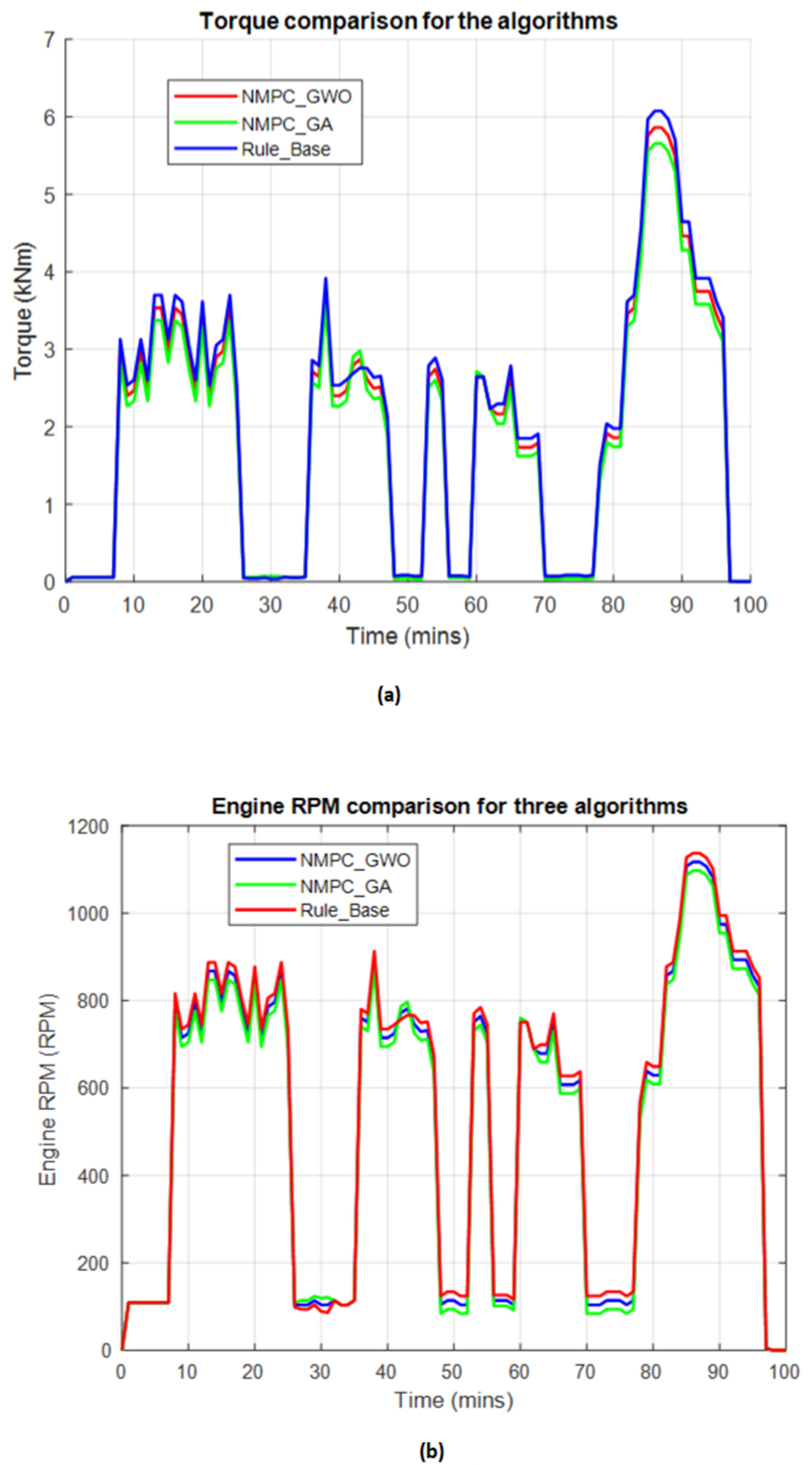
3. Results and Discussion

Figure 11 illustrates the relationship between engine torque and RPM under the three proposed control algorithms. The NMPC-GWO algorithm demonstrates superior performance for the HRES integrated into the tugboat. It achieves the most favorable torque-RPM balance, contributing to reduced fuel consumption and lower emissions. The NMPC-GA algorithm performs moderately well but is hindered by slower convergence and less effective torque distribution. Conversely, the Rule-Based (RB) method yields the worst results due to its non-adaptive framework, which fails to accommodate dynamic disturbances such as wave-induced torque variations, resulting in inefficient fuel usage and higher emissions.

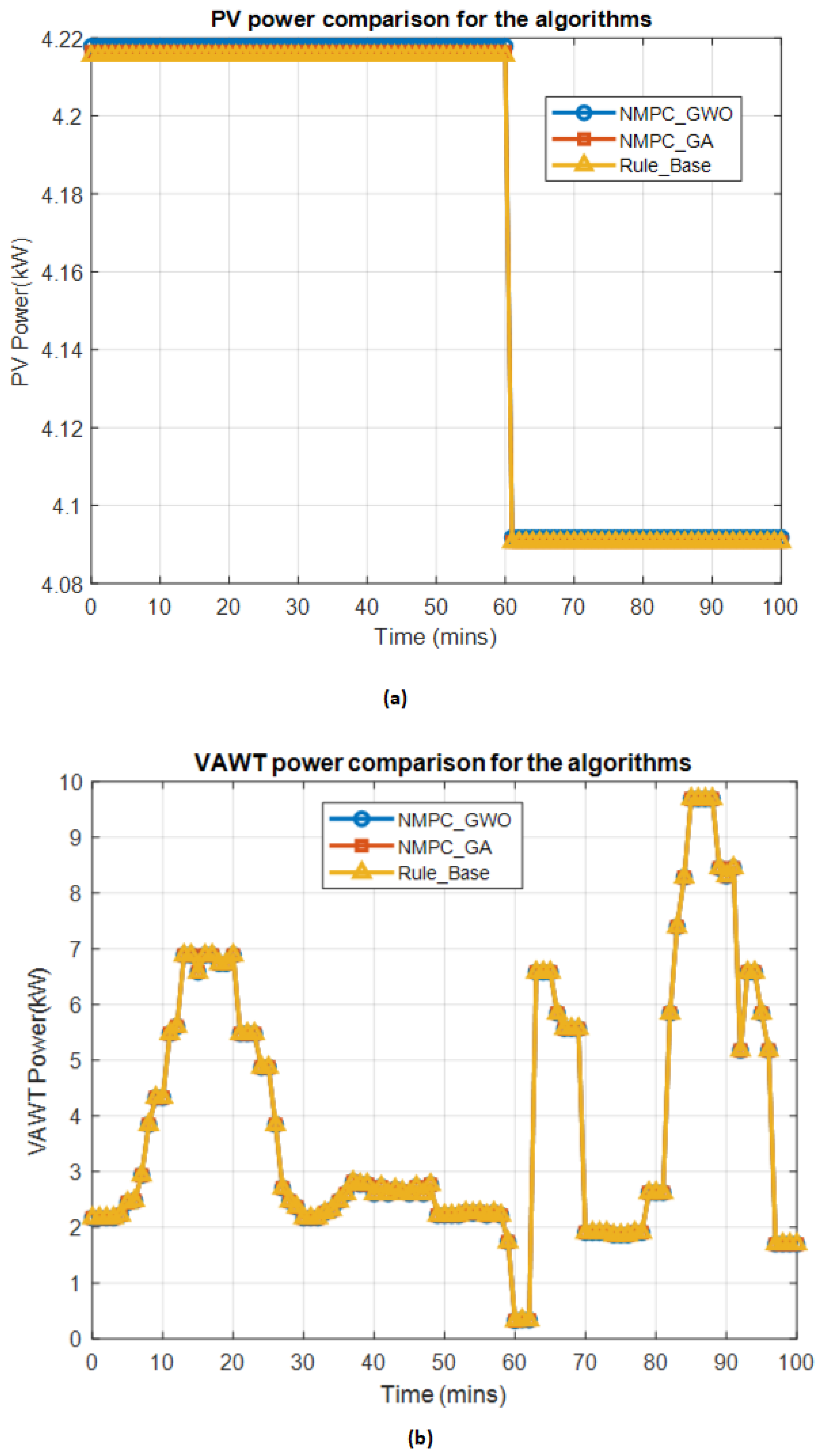
Similarly, Figure 12, Figure 13 and Figure 14 present the comparative simulation results of power generation from photovoltaic (PV) modules, vertical-axis wind turbines (VAWTs), and diesel generator sets (Gensets), along with fuel consumption and battery state of charge (SOC) across the three algorithms. In Figure 12a, the solar power output remained constant across all cases, indicating negligible environmental variability. In contrast, in Figure 12b the wind power exhibited notable fluctuations. Both NMPC-GWO and NMPC-GA algorithms adapted effectively to these variations, outperforming the RB method in wind energy utilization.

Regarding Genset usage in Figure 13a, NMPC-GWO and NMPC-GA demonstrated more efficient load-sharing strategies, thereby minimizing reliance on diesel power. 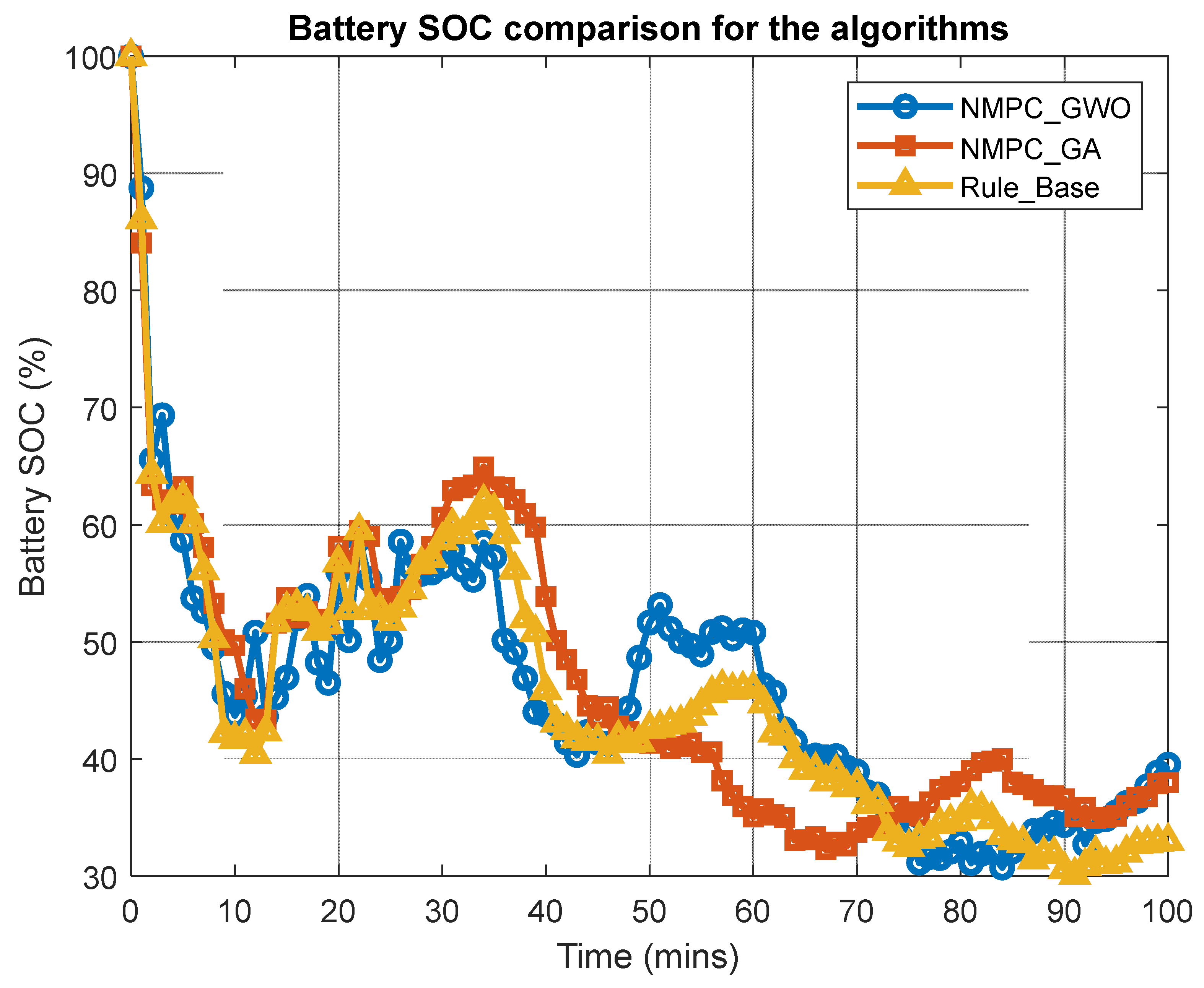The RB method, which utilizes the same hybrid renewable energy system (HRES) platform but employs a static, non-adaptive control strategy, by contrast, exhibited over-dependence on Gensets during suboptimal intervals, resulting in elevated fuel consumption, as shown in Figure 13b. This trend is reflected in the cumulative fuel consumption graph, where the RB approach, though initially efficient, incurred higher total fuel usage due to its static fuel management. In addition, Battery performance in Figure 14 further distinguishes the algorithms. NMPC-GWO and NMPC-GA maintained SOC within an optimal operational range of 50–70%, with NMPC-GWO exhibiting tighter control and better charge balance. The RB method, however, revealed large SOC deviations, indicative of inefficient energy storage control.

Table 2. Results of the proposed algorithms for the HRES fitted on the fully autonomous tugboat.

Algorithms	Total Fuel Consumption (kg)	Total Mass Emission Rate (kg/h)	Emission Cost (EC) (USD/kg)	EEOI (kg/ton-nm)	Total Computational Time (s)
RB	165.661	532.281	10,229.72	3.796	353.153
NMPC-GWO	161.517	518.967	9973.84	3.609	31.601
NMPC-GA	163.476	525.263	10,094.84	3.697	3113.783

quantitatively reinforces these findings. The NMPC-GWO algorithm achieved the lowest fuel consumption (161.517 kg), mass emission rate (518.967 kg/h), emission cost (9973.84 USD), and Energy Efficiency Operational Indicator (EEOI) of 3.609 kg/ton-nm, while also attaining the fastest computational time (31.601 s). The RB method performed the worst across all key performance indicators due to its lack of adaptiveness. NMPC-GA provided intermediate results, constrained by its genetic algorithm’s slower convergence and suboptimal energy allocation.

To quantitatively evaluate the predictive performance of the proposed hybrid Energy Management System (EMS) algorithms, standard statistical regression metrics—Root Mean Squared Error (RMSE); Mean Absolute Error (MAE); and the coefficient of determination (R²)—were computed using a conventional tugboat without HRES integration as the baseline. This baseline reflects a traditional marine propulsion configuration devoid of hybridization or autonomous control, and it serves as a reference point for assessing the gains achieved through predictive control and energy optimization.

Table 3. Performance metrics of NMPC-GWO and NMPC-GA algorithms compared to baseline.

Metric	Algorithm	RMSE	MAE	R2
Fuel Consumption (kg)	NMPC-GWO	11.10	10.74	0.948
	NMPC-GA	9.82	9.58	0.969
Emission Rate (kg/h)	NMPC-GWO	35.26	32.77	0.964
	NMPC-GA	30.44	29.42	0.972
Emission Cost (USD)	NMPC-GWO	692.45	648.96	0.965
	NMPC-GA	607.6	574.31	0.973
EEOI (kg/ton-nm)	NMPC-GWO	0.281	0.259	0.96
	NMPC-GA	0.276	0.265	0.945

presents the comparative results for four primary performance indicators: fuel consumption, emission rate, emission cost, and the Energy Efficiency Operational Indicator (EEOI). These metrics were used to quantify the predictive accuracy and control effectiveness of the NMPC-GWO and NMPC-GA algorithms. In the case of fuel consumption, the NMPC-GA algorithm yielded the lowest RMSE and MAE values, indicating a marginally higher prediction accuracy compared to NMPC-GWO, although both models substantially outperformed the baseline. For emission rate and emission cost predictions, NMPC-GA again demonstrated slightly lower error values and stronger correlation coefficients, affirming its statistical robustness in modeling environmental impact. However, NMPC-GWO exhibited a higher R² value in predicting EEOI, suggesting better alignment with operational efficiency under hybrid-electric propulsion.

It should be noted that the rule-based (RB) method, although implemented on the same hybrid renewable energy platform, lacks the predictive estimation framework required for regression analysis and therefore is excluded from Table 3. Instead, its performance is evaluated through aggregate metrics, as presented earlier in Table 2.

These findings confirm that both predictive algorithms offer statistically significant improvements in modeling accuracy, energy efficiency, and environmental performance when compared to conventional marine propulsion systems. While NMPC-GA showed slightly superior accuracy across most regression metrics, NMPC-GWO remains preferable in real-time maritime applications due to its faster computational speed, robust adaptability to environmental disturbances, and superior control convergence, as demonstrated in the subsequent sensitivity analysis. This underscores the practical suitability of NMPC-GWO for integration into autonomous energy management frameworks in the maritime domain. These promising results motivate the subsequent sensitivity analysis of NMPC-GWO under variable operating parameters.

3.1. Sensitivity Analysis

A sensitivity analysis was conducted to evaluate the robustness and performance adaptability of the proposed HRES governed by the NMPC-GWO algorithm under varying operational conditions in a fully autonomous tugboat. Key system input parameters were varied by ±15%—a range reflecting realistic operational fluctuations—and their effects on total fuel consumption, mass emission rate, emission cost, and EEOI are summarized in

Table 4. Sensitivity analysis of HRES for a fully autonomous tugboat using NMPC-GWO algorithm with impact of operational parameters on fuel consumption, emission rate, emission cost, and EEOI.

Parameters	Percentage Variation	Total Fuel Consumption (kg)	Total Mass Emission Rate (kg/h)	Emission Cost (EC) or Penalty (USD/kg)	EEOI (kg/ton-nm)
Ship speed (knots)	−15%	161.8208	516.6979	9930.23	2.0310
	+15%	163.9685	526.8439	10,125.22	1.7099
Wind speed (knots)	−15%	162.8371	519.9431	9992.60	3.6225
	+15%	161.5115	518.9493	9973.50	3.6086
Ambient temperature (°C)	−15%	161.5217	518.9820	9974.12	3.6091
	+15%	161.5136	518.9561	9973.63	3.6087
Ambient radiation intensity (kW/m2)	−15%	161.5237	518.9885	9974.25	3.6092
	+15%	161.4644	518.7980	9970.59	3.6065
Towing force (tons)	−15%	143.4226	461.7921	8875.01	2.8575
	+15%	459.0715	1475.03	28,348.12	29.15
Ship load (kW)	−15%	161.5049	518.9281	9973.09	3.6083
	+15%	162.6464	522.5959	10,043.58	3.6595

.

Firstly, a 15% reduction in vessel speed led to marginal improvements in energy efficiency, reflected by lower fuel consumption, emissions, and EEOI. This outcome is attributed to reduced propulsion power demand at lower speeds. Conversely, a 15% increase in speed resulted in higher fuel consumption and emissions due to elevated engine loading and reduced propulsion system efficiency.

Secondly, wind speed variations also had a notable impact. A 15% decrease in wind speed diminished the power output from the VAWTs, increasing reliance on the diesel Gensets and battery storage, thereby raising fuel use and emissions. In contrast, a 15% increase in wind speed enhanced wind energy harvesting, improving system efficiency by reducing Genset operation and associated emissions.

Thirdly, ambient temperature and solar radiation exhibited negligible influence on system performance. While minor fluctuations may slightly affect PV output and battery charge–discharge behavior, the overall impact on fuel consumption and emissions was statistically insignificant.

Fourthly, the towing force exhibited a strong correlation with energy demand. A 15% reduction in towing resistance significantly improved fuel efficiency by lowering shaft torque requirements and reducing engine workload. In contrast, an equivalent increase in towing force imposed higher torque demands, thereby escalating fuel usage, emissions, and EEOI.

Lastly, variations in vessel deadweight (load) also influenced system behavior. Reduced load conditions improved fuel economy by enabling greater utilization of renewable energy sources. However, increased load intensified propulsion and auxiliary power demand, thereby increasing dependence on Gensets and resulting in elevated fuel consumption and emissions. These findings highlight the critical importance of adaptive energy management in maintaining operational efficiency under dynamic maritime conditions, validating the NMPC-GWOs suitability for real-time control of hybrid propulsion systems in autonomous vessels.

3.2. Discussion

This study presents a novel multi-objective predictive Energy Management Strategy (EMS) tailored for Hybrid Renewable Energy Systems (HRES) onboard autonomous marine vessels, representing a significant advancement beyond existing methodologies. Unlike prior research that primarily emphasizes minimizing fuel consumption, the proposed approach concurrently optimizes fuel usage, renewable energy integration, and pure-electric sailing duration, achieving a balanced operational performance.

Previous studies, such as those by Roslan et al. [30] and Chan et al. [38] employed Rule-Based (RB) and Equivalent Consumption Minimization Strategy (ECMS) algorithms for hybrid propulsion. However, these conventional methods often neglect the influence of dynamic environmental conditions and system uncertainties. In contrast, the proposed Nonlinear Model Predictive Control integrated with Grey Wolf Optimization (NMPC-GWO) explicitly incorporates such variabilities, resulting in improved system adaptability and efficiency.

Compared to the RB method, which demonstrated suboptimal energy distribution and higher emissions, the NMPC-GWO algorithm consistently outperformed in terms of fuel efficiency, emissions reduction, and effective load balancing, particularly under fluctuating wind conditions. This highlights the critical advantage of adaptive and predictive control strategies over static frameworks in marine hybrid energy management.

Furthermore, the NMPC-GWO results align with findings by Chen et al. [32] on NMPC applications in tugboats but offer enhanced computational efficiency and dynamic responsiveness. The sensitivity analysis reinforced the algorithm’s robustness by demonstrating stable performance across a range of operational scenarios, validating its reliability for real-time implementation in autonomous maritime propulsion systems.

4. Conclusions

This research presents an innovative multi-objective predictive Energy Management System (EMS) for optimizing Hybrid Renewable Energy Systems (HRES) in autonomous ships. By integrating advanced predictive-metaheuristic algorithms—namely NMPC-GWO, NMPC-GA, and Rule-Based (RB) methods—the study addresses fuel consumption, emissions, renewable energy integration, and pure-electric sailing duration within a unified framework. A realistic modeling approach incorporates random wave effects on propeller load torque, with state estimation supported by an Extended Kalman Filter to improve prediction accuracy.

The NMPC-GWO algorithm demonstrated superior performance in fuel efficiency, emission reduction, and computational speed, outperforming NMPC-GA and RB methods. This superiority was quantitatively confirmed through standard regression metrics—Root Mean Squared Error (RMSE), Mean Absolute Error (MAE), and coefficient of determination (R²)—which highlighted NMPC-GWOs accuracy and reliability in predicting fuel consumption and emissions compared to a conventional diesel-only baseline. Sensitivity analyses further verified the robustness and adaptability of the NMPC-GWO under varying operational parameters such as vessel speed, wind conditions, and towing forces, confirming its suitability for real-time energy management in dynamic maritime environments.

Ultimately, this study offers a comprehensive and adaptable energy management framework that advances the integration of renewable energy sources in autonomous vessel propulsion and power systems.

For future work, real-world validation through experimental testing or sea trials on autonomous vessels is recommended to assess the practical performance of the proposed system. Additionally, the EMS framework can be extended to other vessel types, such as ferries and cargo ships, to evaluate its scalability. Further enhancement may include integrating alternative renewable energy sources like fuel cells or wave energy converters into the HRES model for broader applicability and improved sustainability. Moreover, efforts will focus on optimizing the computational efficiency of the NMPC-GWO algorithm to enable real-time implementation in dynamic maritime environments.