
Performance Evaluation of Combined Wind-Assisted Propulsion and Organic Rankine Cycle Systems in Ships


Abstract
1. Introduction
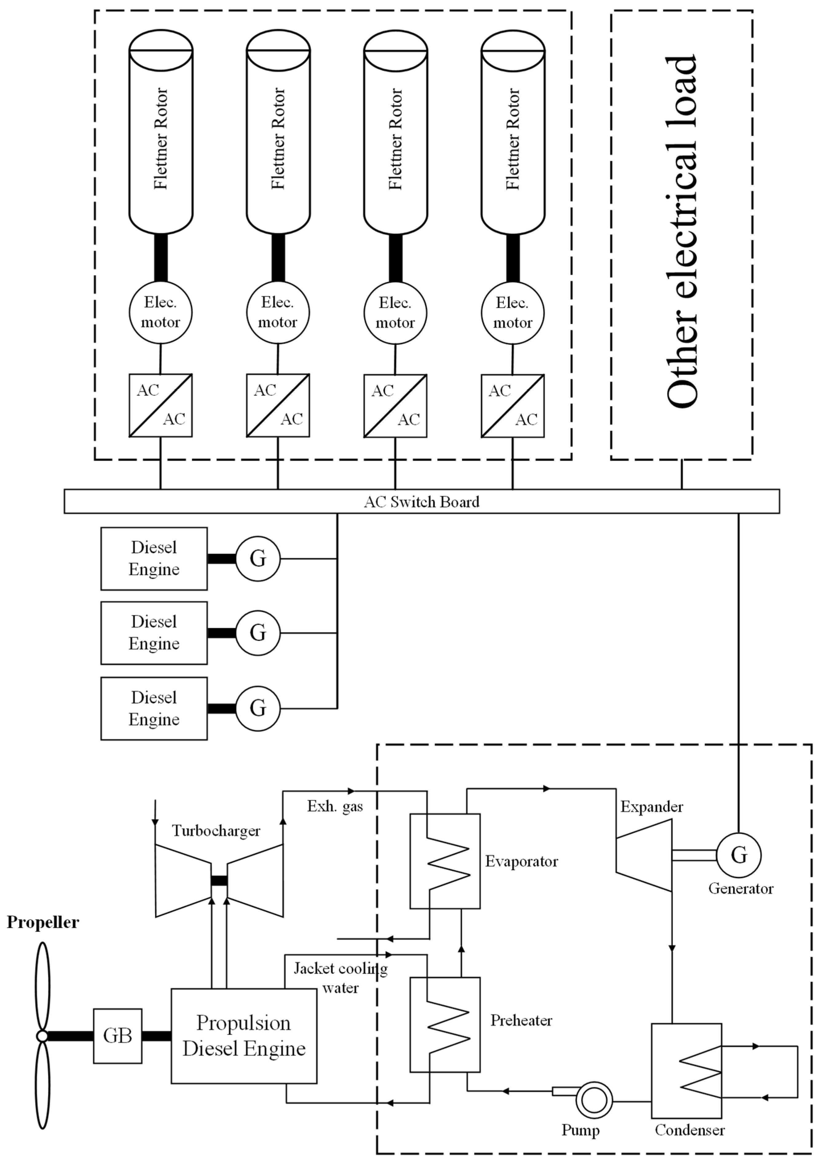
2. Mathematical Model of the WAPS and ORC Technologies
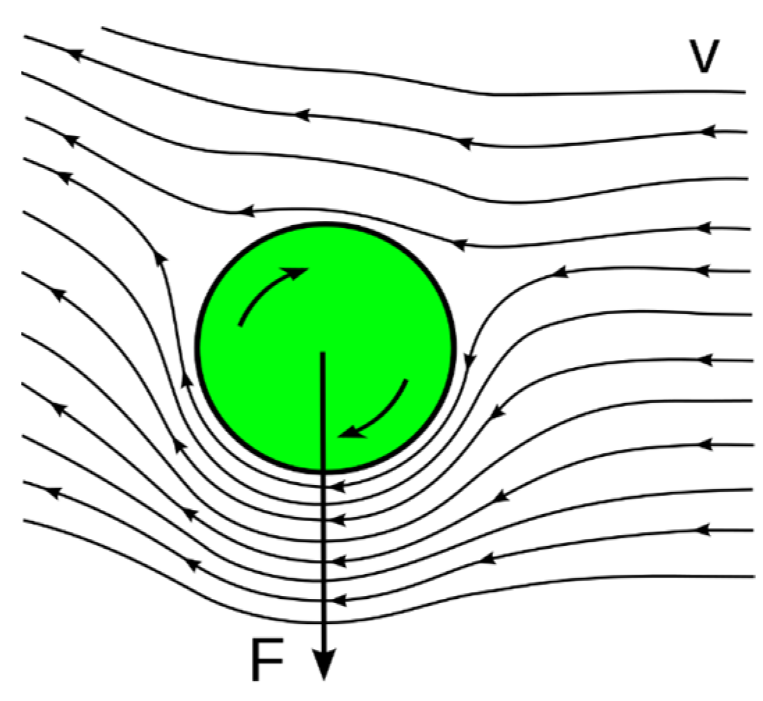
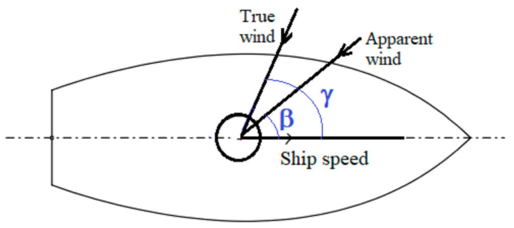
2.1. Wind-Assisted Propulsion System
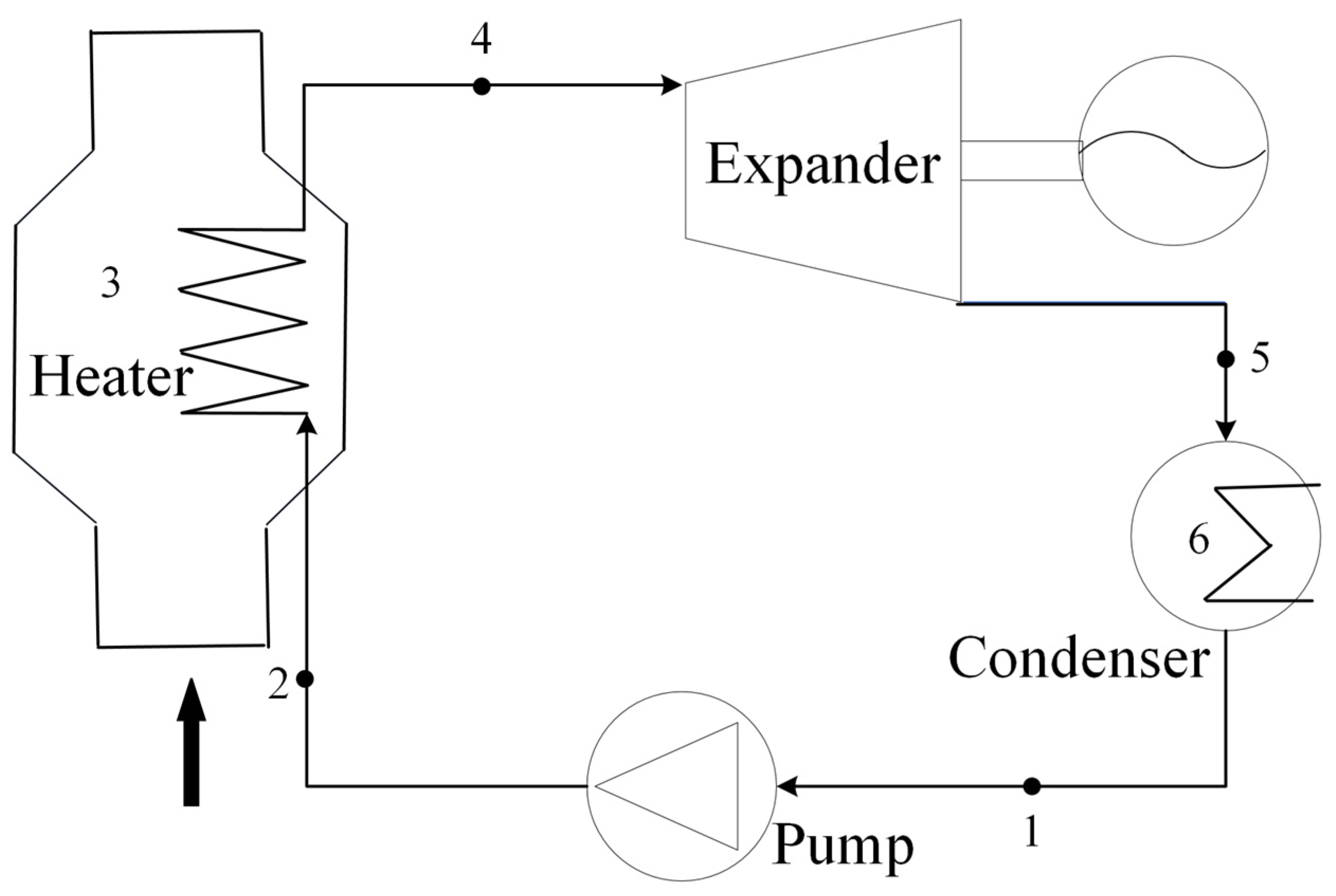
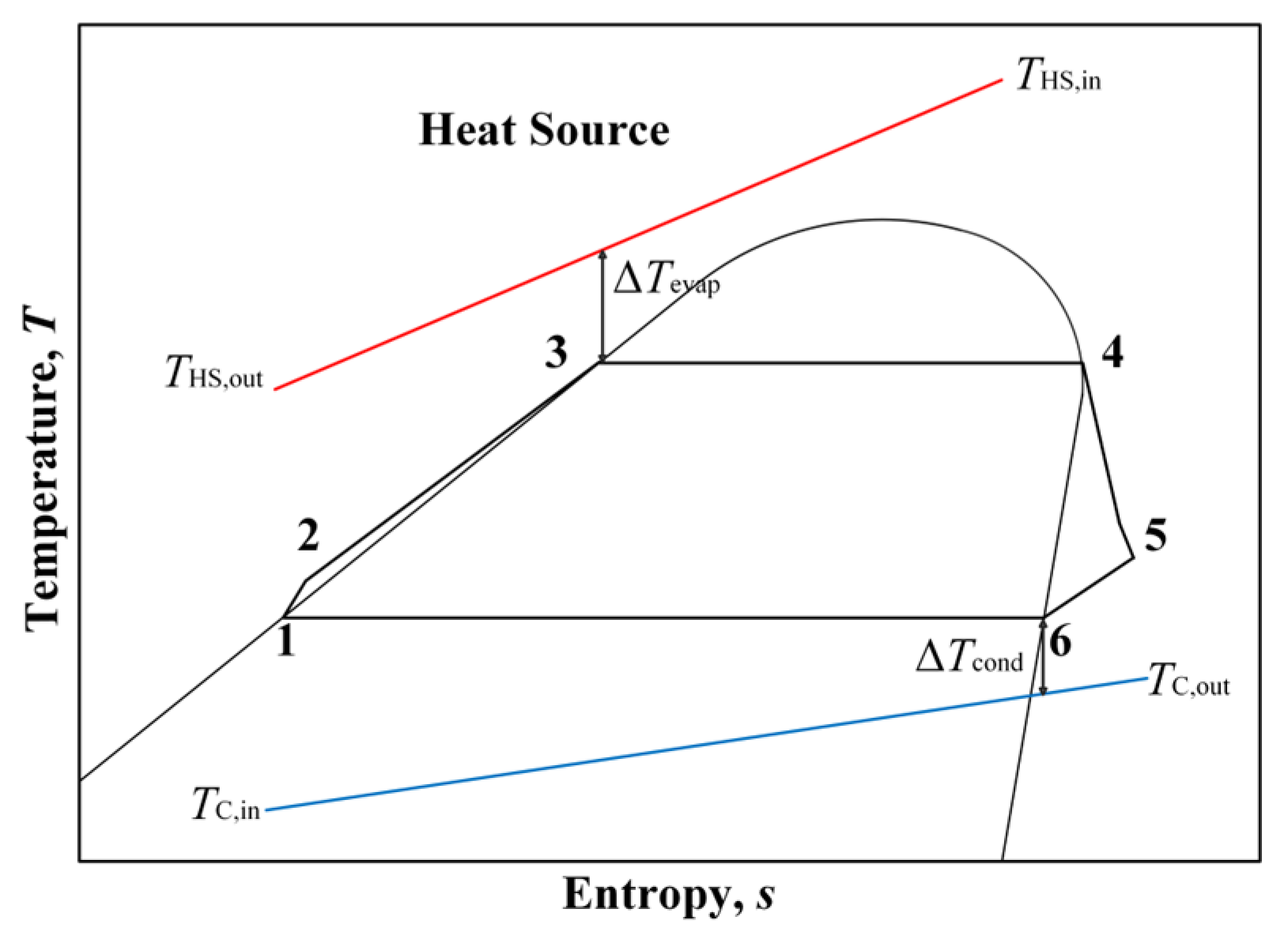
2.2. Organic Rankine Cycle
2.3. Model Verification
3. Ship Fuel Consumption Model
3.1. Fuel Consumption Model for Ships Without Any Energy-Saving Technologies
3.2. Fuel Consumption Model for Ships with WAPS
3.3. Fuel Consumption Model for Ships with the ORC
3.4. Fuel Consumption Model for Ships with WAPS and the ORC
4. Case Study
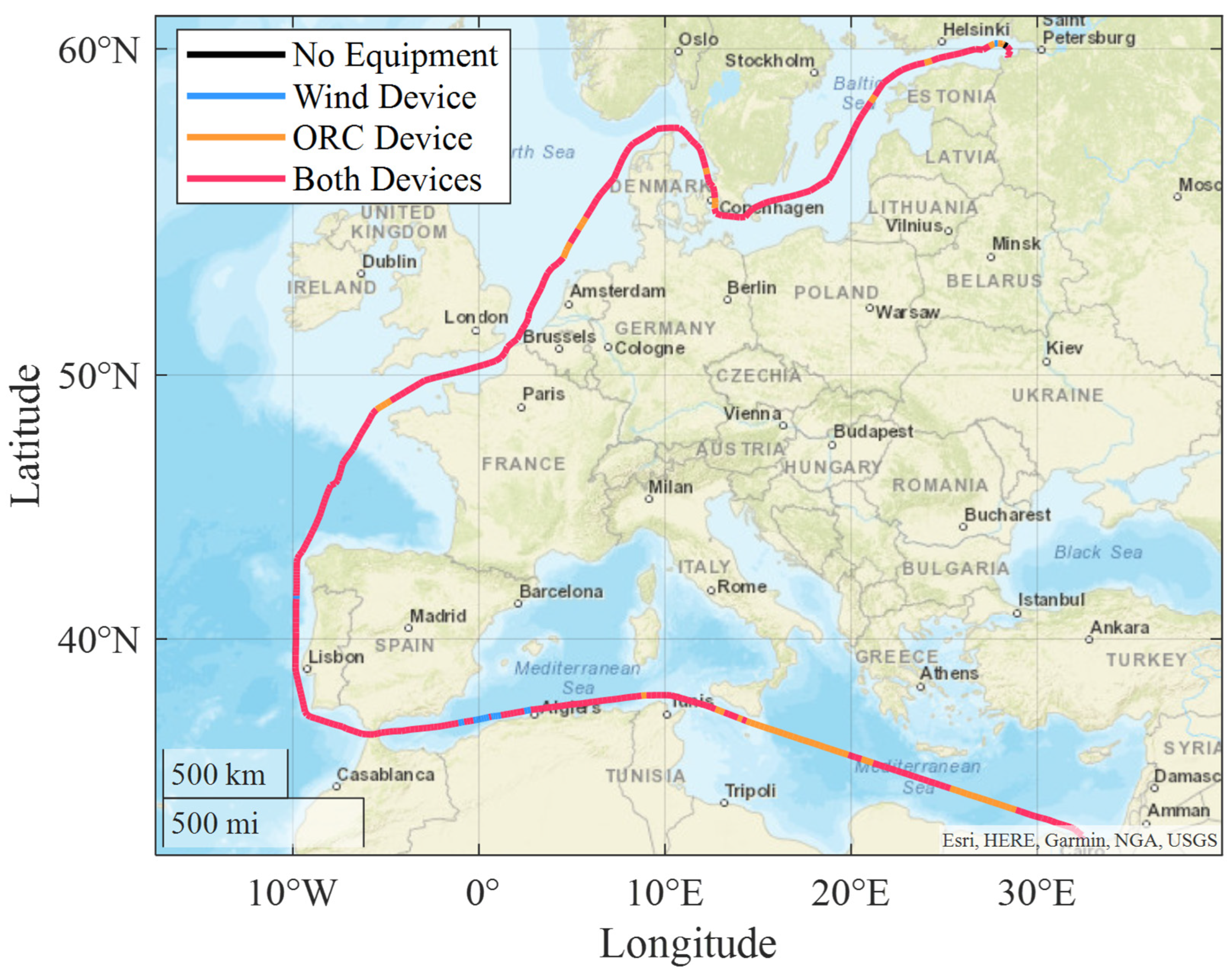
4.1. Study Case Description
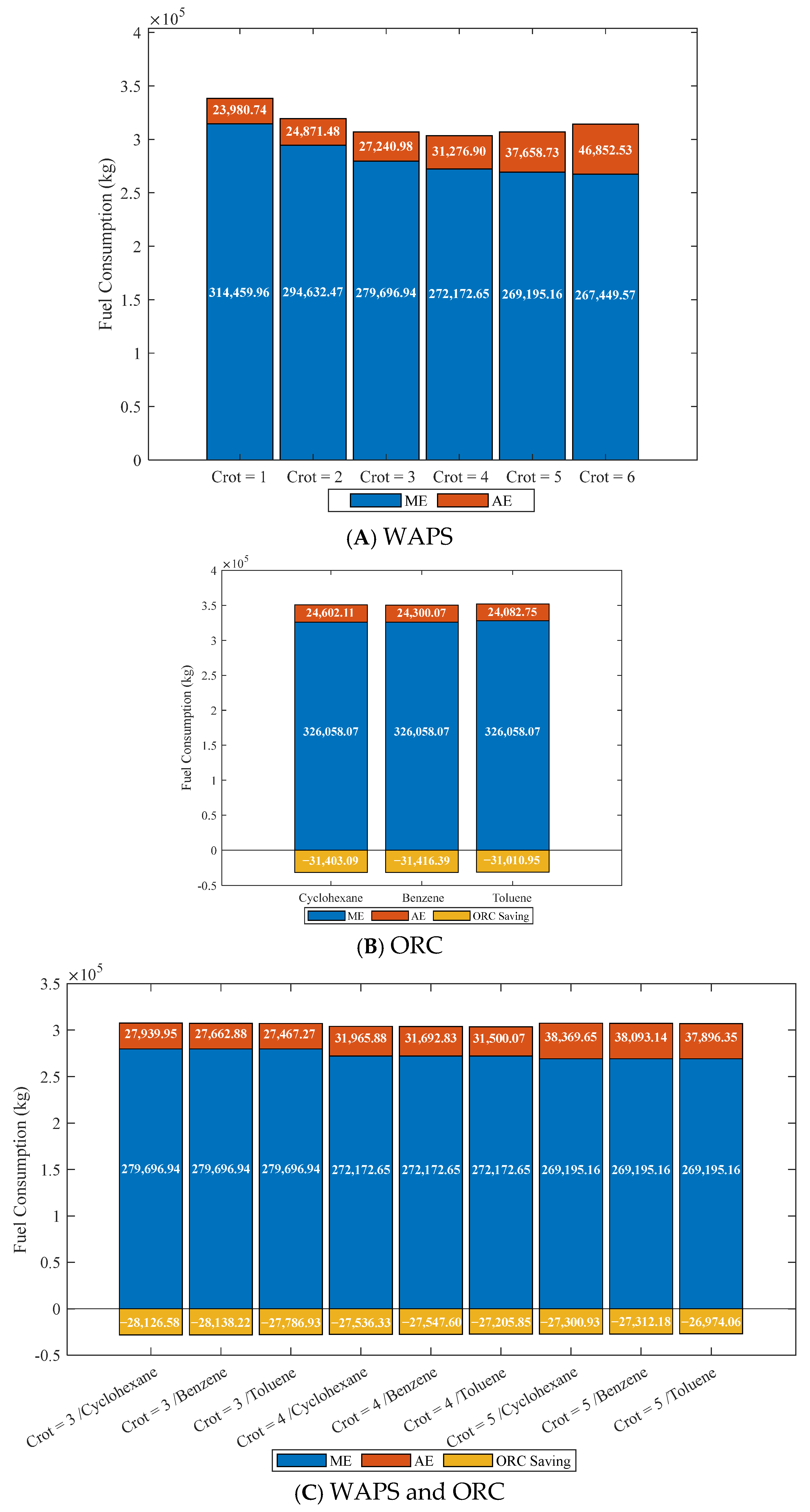
4.2. The Impact of Energy-Saving Technology Combinations on ME and D/Gs Fuel Consumption
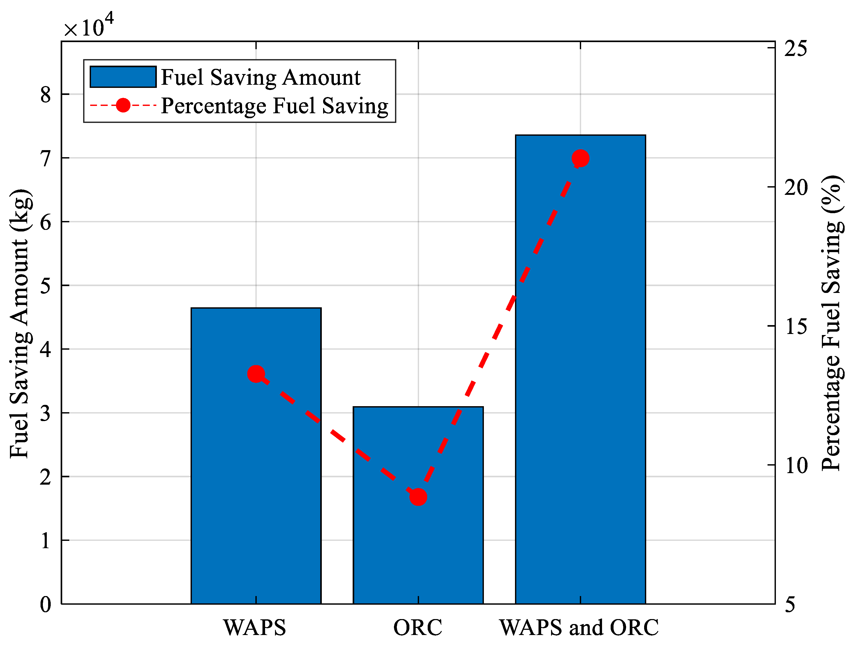
4.3. Comparison of Fuel-Saving Effects of Energy-Saving Technology Combinations
5. Discussion
6. Conclusions
- (1)
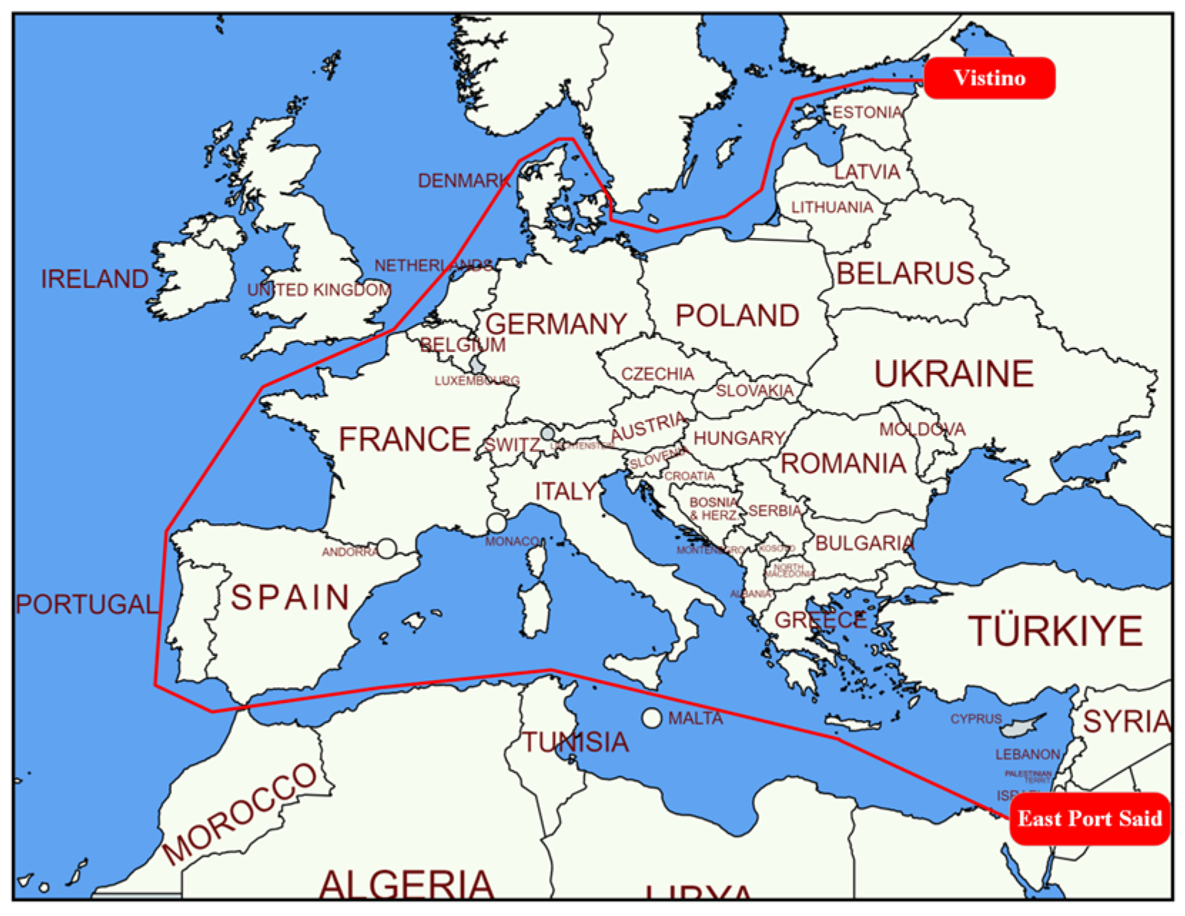
- A combination of two energy saving is defined, and the rotation coefficient of WAPS is set to 4, and the fuel saving effect is best when benzene is used as the working fluid. A voyage from the East Port Said to Vistino can save 73.58 t of fuel, reducing the fuel consumption of the whole ship by 21.03%.
- (2)
- The fuel saving effects of using WAPS and ORC individually, as well as their combination, was compared. The voyage fuel savings rates for WAPS, ORC, and the combination of WAPS and ORC were 8.85%, 13.27%, and 21.03%, respectively.
- (3)
- When using WAPS, a large amount of electricity is required to drive the Flettner rotor. Especially when the rotor rotation coefficient is large or the wind speed is high, additional D/Gs may be needed to drive it.
- (4)
- When green technology is used, the equivalent fuel consumption generated by ORC will be reduced. This is because of the load on the main engine is reduced, resulting in a reduction in the net power generated by ORC. At the same time, when using new technologies, the fuel consumption of the D/Gs is significantly higher than when not using technologies. Therefore, when evaluating the impact of green technologies on the efficiency of main engines, the overall fuel consumption should be considered at the same time to obtain more meaningful results.
Author Contributions
Funding
Data Availability Statement
Conflicts of Interest
Abbreviations
| ASHRAE 34 | American Society of Heating, Refrigerating and Air-Conditioning Engineers Standard 34a—Refrigerant safety group classification |
| CII | Carbon intensity index |
| D/G | Diesel generator |
| EEDI | Energy efficiency design index |
| EEXI | Energy efficiency existing index |
| GWP | Global warming potential |
| IMO | International Maritime Organization |
| ME | Main engine |
| ODP | Ozone depletion potential |
| ORC | Organic Rankine cycle |
| SFOC | Specific fuel oil consumption |
| SR | Spin ratio |
| WAPS | Wind-assisted propulsion system |
Appendix A

| Date | Speed (Knots) | Course (°) | Latitude (°) | Longitude (°) | TWS (Knots) | TWA (°) |
|---|---|---|---|---|---|---|
| 20-Feb-24 | 12.62 | 238.00 | 31.78 | 31.60 | 10.91 | 131.44 |
| 21-Feb-24 | 13.08 | 287.00 | 32.95 | 27.57 | 4.91 | 200.82 |
| 22-Feb-24 | 12.92 | 287.75 | 34.60 | 21.56 | 6.05 | 186.73 |
| 23-Feb-24 | 12.58 | 288.88 | 36.24 | 15.51 | 12.11 | 154.86 |
| 24-Feb-24 | 11.83 | 272.79 | 37.50 | 9.64 | 14.89 | 105.54 |
| 25-Feb-24 | 10.25 | 261.21 | 37.12 | 3.90 | 23.39 | 93.09 |
| 26-Feb-24 | 6.89 | 259.29 | 36.60 | −0.07 | 28.01 | 84.75 |
| 27-Feb-24 | 10.60 | 267.08 | 36.12 | −4.47 | 20.38 | 134.50 |
| 28-Feb-24 | 10.57 | 311.67 | 37.46 | −9.13 | 21.25 | 125.51 |
| 29-Feb-24 | 8.74 | 120.46 | 41.17 | −9.82 | 20.20 | 129.24 |
| 01-Mar-24 | 8.36 | 35.46 | 44.36 | −8.94 | 23.68 | 192.45 |
| 02-Mar-24 | 9.88 | 32.71 | 47.40 | −6.72 | 11.12 | 147.72 |
| 03-Mar-24 | 13.07 | 61.75 | 50.09 | −1.33 | 6.45 | 262.41 |
| 04-Mar-24 | 12.78 | 28.42 | 53.58 | 4.14 | 8.68 | 182.58 |
| 05-Mar-24 | 11.13 | 76.04 | 57.17 | 9.23 | 20.31 | 126.75 |
| 06-Mar-24 | 10.53 | 117.38 | 55.72 | 13.57 | 15.25 | 124.62 |
| 07-Mar-24 | 12.87 | 42.08 | 57.39 | 19.70 | 7.08 | 83.39 |
| 08-Mar-24 | 9.32 | 98.41 | 59.88 | 26.38 | 7.74 | 120.72 |
References
- IMO. IMO Regulations to Introduce Carbon Intensity Measures Enter into Force on 1 November 2022. 2022. Available online: https://www.imo.org/en/MediaCentre/PressBriefings/pages/CII-and-EEXI-entry-into-force.aspx (accessed on 1 July 2024).
- Vasilev, M.; Kalajdžić, M.; Momčilović, N. On energy efficiency of tankers: EEDI, EEXI and CII. Ocean Eng. 2025, 317, 120028. [Google Scholar] [CrossRef]
- Jimenez, V.J.; Kim, H.; Munim, Z.H. A review of ship energy efficiency research and directions towards emission reduction in the maritime industry. J. Clean. Prod. 2022, 366, 132888. [Google Scholar] [CrossRef]
- Wang, Z.; Wang, K.; Huang, L.; Chen, J.; Chen, W. Dynamic optimisation method of ship speed based on sea condition recognition. J. Harbin Eng. Univ. 2022, 43, 488–494. [Google Scholar]
- Yang, H.; Ren, F.; Yin, J.; Wang, S.; Rafi, U.K. Tramp Ship Routing and Scheduling with Integrated Carbon Intensity Indicator (CII) Optimization. J. Mar. Sci. Eng. 2025, 13, 752. [Google Scholar] [CrossRef]
- Kim, Y.R.; Steen, S. Potential energy savings of air lubrication technology on merchant ships. Int. J. Nav. Archit. 2023, 15, 100530. [Google Scholar] [CrossRef]
- Oyuela, S.; Ojeda, H.R.D.; Arribas, F.P.; Alejandro, D.O.; Sosa, R. Investigating fishing vessel hydrodynamics by using EFD and CFD tools, with focus on total ship resistance and its components. J. Mar. Sci. Eng. 2024, 12, 622. [Google Scholar] [CrossRef]
- Rowin, W.A.; Asha, A.B.; Narain, R.; Ghaemi, S. A novel approach for drag reduction using polymer coating. Ocean Eng. 2021, 240, 109895. [Google Scholar] [CrossRef]
- Zhang, Y.; Sun, L.; Sun, W.; Ma, F.; Xiao, R.; Wu, Y.; Huang, H. Bilevel Optimal Infrastructure Planning Method for the Inland Battery Swapping Stations and Battery-Powered Ships. Tsinghua Sci. Technol. 2024, 29, 1323–1340. [Google Scholar] [CrossRef]
- Liu, H.; Fan, A.; Li, Y.; Bucknall, R.; Vladimir, N. Multi-objective hierarchical energy management strategy for fuel cell/battery hybrid power ships. Appl. Energy 2025, 379, 124981. [Google Scholar] [CrossRef]
- Čalić, A.; Jurić, Z.; Katalinić, M. Impact of Wind-Assisted Propulsion on Fuel Savings and Propeller Efficiency: A Case Study. J. Mar. Sci. Eng. 2024, 12, 2100. [Google Scholar] [CrossRef]
- Chen, W.; Xue, S.; Lyu, L.; Luo, W.; Yu, W. Energy saving analysis of a marine main engine during the whole voyage utilizing an organic rankine cycle system to recover waste heat. J. Mar. Sci. Eng. 2023, 11, 103. [Google Scholar] [CrossRef]
- Zhao, F.; Wang, Z.; Wang, D.; Han, F.; Ji, Y.; Cai, W. Top level design and evaluation of advanced low/zero carbon fuel ships power technology. Energy Rep. 2022, 8, 336–344. [Google Scholar] [CrossRef]
- Chou, T.; Kosmas, V.; Acciaro, M.; Renken, K. A comeback of wind power in shipping: An economic and operational review on the wind-assisted ship propulsion technology. Sustainability 2021, 13, 1880. [Google Scholar] [CrossRef]
- Marcin, K.; Sosnowski, M. Review of Wind-Assisted Propulsion Systems in Maritime Transport. Energies 2025, 18, 897. [Google Scholar] [CrossRef]
- Seddiek, I.S.; Ammar, N.R. Harnessing wind energy on merchant ships: Case study Flettner rotors onboard bulk carriers. Environ. Sci. Pollut. Res. Environ. Sci. Pollut. Res. Int. 2021, 28, 32695–32707. [Google Scholar] [CrossRef]
- Li, B.; Zhang, R.; Zhang, B.; Yang, Q.; Guo, C. An assisted propulsion device of vessel utilizing wind energy based on Magnus effect. Appl. Ocean Res. 2021, 114, 102788. [Google Scholar] [CrossRef]
- Ammar, N.R.; Seddiek, I.S. Wind assisted propulsion system onboard ships: Case study Flettner rotors. Sh. Offshore Struct. 2022, 17, 1616–1627. [Google Scholar] [CrossRef]
- Baldi, F.; Ahlgren, F.; Nguyen, T.V.; Thern, M.; Andersson, K. Energy and exergy analysis of a cruise ship. Energies 2018, 11, 2508. [Google Scholar] [CrossRef]
- Lebedevas, S.; Čepaitis, T. Complex use of the main marine diesel engine high-and low-temperature waste heat in the organic rankine cycle. J. Mar. Sci. Eng. 2024, 12, 521. [Google Scholar] [CrossRef]
- Mondejar, M.E.; Ahlgren, F.; Thern, M.; Genrup, M. Quasi-steady state simulation of an organic Rankine cycle for waste heat recovery in a passenger vessel. Appl. Energy 2017, 185, 1324–1335. [Google Scholar] [CrossRef]
- Konur, O.; Yuksel, O.; Korkmaz, S.A.; Colpan, C.O.; Saatcioglu, O.Y.; Koseoglu, B. Operation-dependent exergetic sustainability assessment and environmental analysis on a large tanker ship utilizing Organic Rankine cycle system. Energy 2023, 262, 125477. [Google Scholar] [CrossRef]
- Jost, S. A review of the Magnus effect in aeronautics. Prog. Aerosp. Sci. 2012, 55, 17–45. [Google Scholar]
- Lele, A.; Rao, K.V.S. Net power generated by Flettner rotor for different values of wind speed and ship speed. In Proceedings of the 2017 International Conference on Circuit, Power and Computing Technologies (ICCPCT), Kollam, India, 20–21 April 2017; pp. 1–6. [Google Scholar]
- Tillig, F.; Ringsberg, J.W. Design, operation and analysis of wind-assisted cargo ships. Ocean Eng. 2020, 211, 107603. [Google Scholar] [CrossRef]
- Pirouzfar, V.; Saleh, S.; Su, C.H. Working fluid selection of organic Rankine cycle with considering the technical, economic and energy analysis. J. Therm. Anal. Calorim. 2024, 149, 9819–9829. [Google Scholar] [CrossRef]
- Song, J.; Song, Y.; Gu, C. Thermodynamic analysis and performance optimization of an Organic Rankine Cycle (ORC) waste heat recovery system for marine diesel engines. Energy 2015, 82, 976–985. [Google Scholar] [CrossRef]
- Holtrop, J.; Mennen, G.G.J. An approximate power prediction method. Int. Shipbuild. Prog. 1982, 29, 166–170. [Google Scholar] [CrossRef]
- ITTC, Full Scale Measurements—Speed and Power Trials—Analysis of Speed/Power Trial Data. Available online: https://ittc.info/media/1363/75-04-01-012.pdf (accessed on 15 July 2024).
- MAN. CEAS Engine Calculations. Available online: https://www.man-es.com/marine/products/planning-tools-and-downloads/ceas-engine-calculations (accessed on 10 June 2025).
- Generator Source. Approximate Diesel Generator Fuel Consumption Chart. Available online: https://www.generatorsource.com/Diesel_Fuel_Consumption.aspx (accessed on 10 June 2024).
- IMO. Fourth IMO GHG Study 2020. 2020. Available online: https://www.imo.org/en/OurWork/Environment/Pages/Fourth-IMO-Greenhouse-Gas-Study-2020.aspx (accessed on 1 July 2024).
- Yiğit, K. Evaluation of energy efficiency potentials from generator operations on vessels. Energy 2022, 257, 124687. [Google Scholar] [CrossRef]


| y = 70° | y = 180° | y = 260° | |||||||
|---|---|---|---|---|---|---|---|---|---|
| Paper | Results | Error (%) | Paper | Results | Error (%) | Paper | Results | Error (%) | |
| Crot = 2 | 40.36 | 40.34 | 0.05 | −4.73 | −4.74 | 0.21 | 54.18 | 54.14 | 0.07 |
| Crot = 3 | 39.48 | 39.45 | 0.08 | −8.58 | −8.59 | 0.17 | 52.31 | 52.27 | 0.08 |
| Crot = 4 | 37.82 | 37.80 | 0.05 | −15.76 | −15.79 | 0.19 | 48.81 | 48.76 | 0.10 |
| Crot = 5 | 35.18 | 35.15 | 0.09 | −27.22 | −27.26 | 0.15 | 43.23 | 43.17 | 0.14 |
| Crot = 6 | 31.34 | 31.30 | 0.13 | −43.87 | −43.94 | 0.16 | 35.12 | 35.02 | 0.20 |
| Working Fluid | Molecule Weight (g/mol) | Normal Boiling Point (K) | Critical Temperature (K) | Critical Pressure (kPa) | GWP | ODP | ASHRAE 34 |
|---|---|---|---|---|---|---|---|
| Cyclohexane | 84.16 | 353.9 | 553.6 | 4075.0 | −4.74 | 0 | A3 |
| Benzene | 78.11 | 353.2 | 562.1 | 4894.0 | −8.59 | 0 | B2 |
| Toluene | 92.14 | 383.8 | 591.8 | 4126.3 | 43.94 | 0 | A3 |
| Type of Working Fluid | Cyclohexane | Benzene | Toluene | ||||||
|---|---|---|---|---|---|---|---|---|---|
| Paper | Results | Error (%) | Paper | Results | Error (%) | Paper | Results | Error (%) | |
| Evaporation temperature (K) | 518.3 | 518.4 | 0.02 | 479.8 | 479.7 | 0.02 | 477.2 | 479.7 | 0.52 |
| Working fluid mass flow (kg/s) | 0.62 | 0.602 | 3.23 | 0.68 | 0.67 | 1.47 | 0.67 | 0.67 | 0 |
| System net power (kW) | 90.1 | 91.67 | 1.74 | 90.8 | 91.71 | 1.00 | 89.2 | 89.65 | 0.50 |
| System thermal efficiency (%) | 21.2 | 21.17 | 0.14 | 21.3 | 21.41 | 0.52 | 21 | 21.29 | 1.38 |
| System | Step | Description | Reference |
|---|---|---|---|
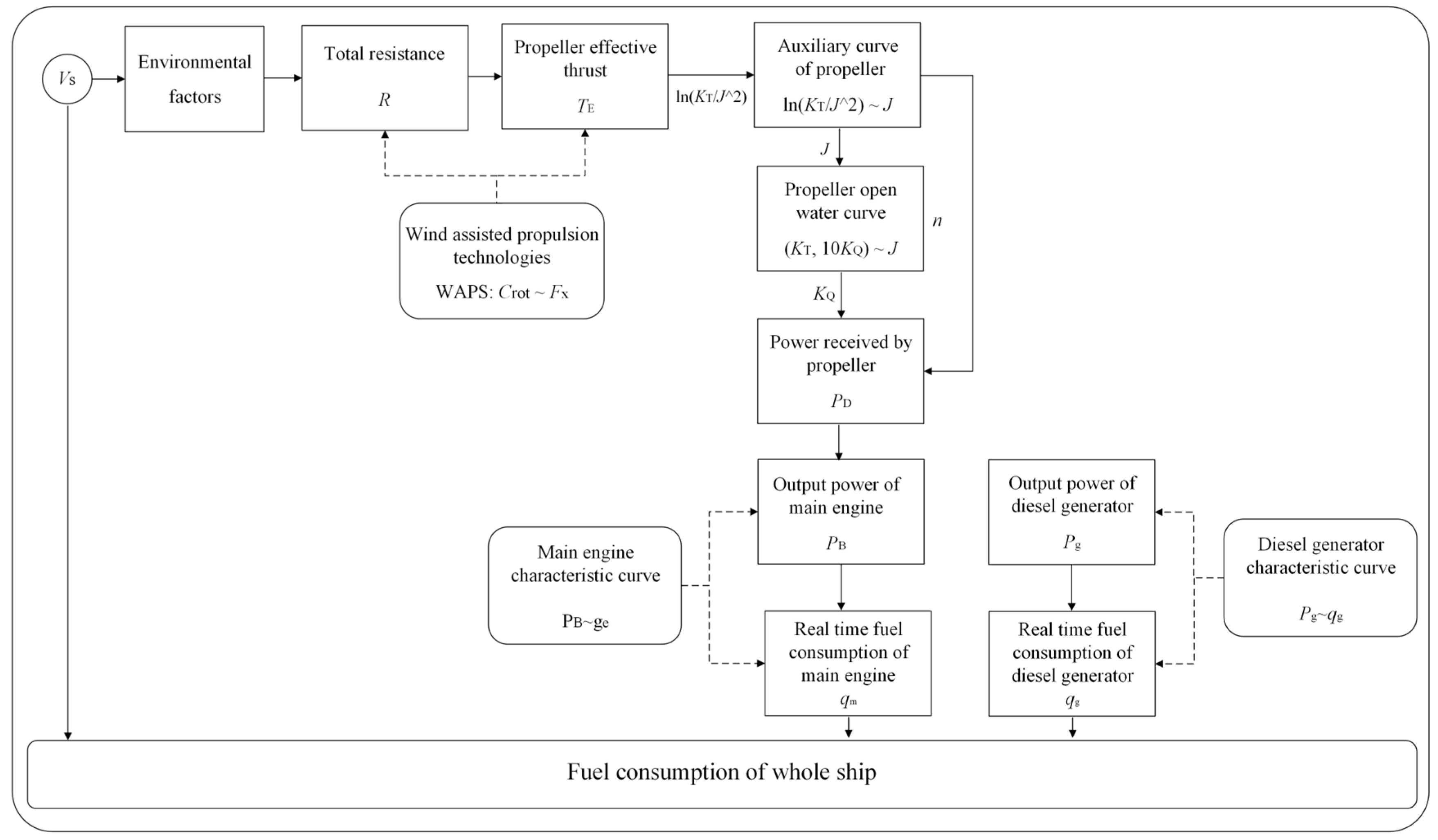
| ME | (1) | Calculate the ship hull resistance according to environmental factors and ship sailing speed. | Formulas (16) to (19) |
| (2) | Calculate the effective thrust. | Formulas (20) and (35) | |
| (3) | Obtain the propeller advance coefficient and the torque coefficient. | Formula (29), Figure 5 | |
| (4) | Obtain the propeller speed. | Formula (26) | |
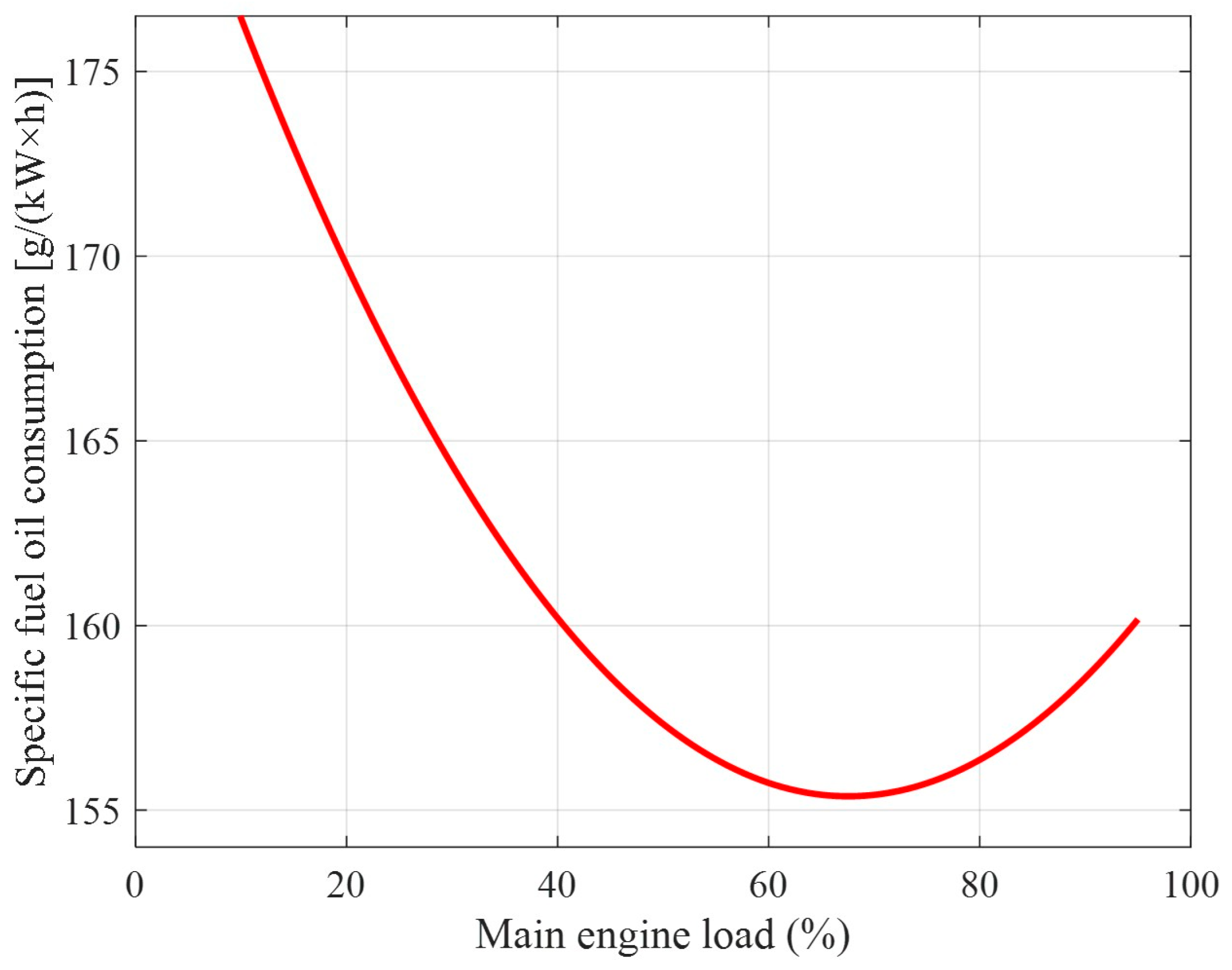
| (5) | Calculate the main engine output power and obtain the SFOC. | Formula (28), Figure 6 | |
| (6) | Calculate the main engine energy consumption. | Formula (31) | |
| D/Gs | (1) | Determine the D/G power demand based on the vessel type, size, activity. | Formula (32) |
| (2) | Calculate the electrical load for different technology combinations. | Formulas (37), (39) and (40) | |
| (3) | Calculate the D/G energy consumption using consumption rates. | Figure 7, Formula (33) | |
| ORC savings | (1) | Calculate the equivalent fuel consumption savings using D/G consumption rates for ORC-generated electricity. | Figure 7, Formula (38) |
| Ship Parameters | ME and D/G |
|---|---|
| Length: 190 m | ME model: 6S50ME-C10.7 |
| Breadth: 32.26 m | ME MCR power: 1 × 9500 kW |
| Deadweight tonnage: 53,000 t | ME speed: 125 RPM |
| Design draft: 11.5 m | D/G MCR power: 3 × 500 kW |
| Vessel | Power Demand (kW) | ||||
|---|---|---|---|---|---|
| Type | Size (dwt) | Berth | Anchor | Man. | Sea |
| Bulk carrier | 35,000–59,999 | 150 | 250 | 680 | 260 |
Disclaimer/Publisher’s Note: The statements, opinions and data contained in all publications are solely those of the individual author(s) and contributor(s) and not of MDPI and/or the editor(s). MDPI and/or the editor(s) disclaim responsibility for any injury to people or property resulting from any ideas, methods, instructions or products referred to in the content. |
© 2025 by the authors. Licensee MDPI, Basel, Switzerland. This article is an open access article distributed under the terms and conditions of the Creative Commons Attribution (CC BY) license (https://creativecommons.org/licenses/by/4.0/).
Share and Cite
Zhao, S.; Pazouki, K.; Norman, R. Performance Evaluation of Combined Wind-Assisted Propulsion and Organic Rankine Cycle Systems in Ships. J. Mar. Sci. Eng. 2025, 13, 1287. https://doi.org/10.3390/jmse13071287
Zhao S, Pazouki K, Norman R. Performance Evaluation of Combined Wind-Assisted Propulsion and Organic Rankine Cycle Systems in Ships. Journal of Marine Science and Engineering. 2025; 13(7):1287. https://doi.org/10.3390/jmse13071287
Chicago/Turabian StyleZhao, Shibo, Kayvan Pazouki, and Rosemary Norman. 2025. "Performance Evaluation of Combined Wind-Assisted Propulsion and Organic Rankine Cycle Systems in Ships" Journal of Marine Science and Engineering 13, no. 7: 1287. https://doi.org/10.3390/jmse13071287
APA StyleZhao, S., Pazouki, K., & Norman, R. (2025). Performance Evaluation of Combined Wind-Assisted Propulsion and Organic Rankine Cycle Systems in Ships. Journal of Marine Science and Engineering, 13(7), 1287. https://doi.org/10.3390/jmse13071287