Energy-Optimized Path Planning for Fully Actuated AUVs in Complex 3D Environments

Abstract

This paper presents an energy-optimized path planning approach for fully actuated autonomous underwater vehicles (AUVs) in three-dimensional ocean environments to enhance their operational range and endurance. A fully actuated AUV is characterized by its high degrees of freedom and precise controllability. Using real terrain data, we construct environmental models incorporating a Lamb vortex and random obstacles. We develop a mathematical model of the AUV’s total energy consumption, accounting for constraints imposed by its fully actuated design and extensive maneuverability. To minimize energy usage, we propose an energy-optimized path planning algorithm that combines energy-optimized particle swarm optimization (EOPSO) and sequential quadratic programming (SQP). The proposed method identifies the optimal path for energy consumption and the corresponding optimal surge speed. The efficacy of the algorithm in optimizing the total energy consumption of the AUV is demonstrated through the simulation of various scenarios. In comparison to other algorithms, paths planned by this algorithm are shown to have superior robustness and optimized energy consumption.

1. Introduction

With the exploration of the marine environment and the exploitation of underwater resources, autonomous underwater observation technology is constantly advancing. Autonomous underwater vehicles (AUVs) have been widely used in the fields of marine pipeline detection [1], environmental monitoring [2], and ecosystem data collection [3], as well as for military purposes [4]. Due to the complexity of the marine environment, the effective utilization of the marine environmental elements and the avoidance of various obstacles in the ocean are the keys to achieving autonomous navigation; thus, path planning is becoming an important aspect of the underwater missions performed by AUVs.

Due to the limited energy capacity of the AUV, it must return to an underwater base station for recharging or to be recovered for energy replenishment after operations. Consequently, the implementation of a low-energy trajectory can prolong the mission endurance and expand the operational range of the AUV, thereby enhancing the efficiency of energy utilization. This is of paramount importance for long-duration, wide-ranging AUV missions, which are the primary focus of the research presented in this paper.

To develop energy-efficient navigation strategies, it is essential to understand the influence of ocean currents. Scholars have proposed numerous path-planning methods that integrate ocean currents as a key environmental factor. Garau used an A* algorithm to search for a navigation path with minimum energy consumption in a large-scale non-uniform current environment [5]. Yao proposed a continuous-direction path planning method for AUVs based on an edge search algorithm [6]. The proposed method does not fix path waypoints exactly but instead uses currents to reduce energy consumption. Yao and Wang constructed a cost function in terms of running time and consumed energy by modeling the eddy field and the current field. They regarded a strong current field as an obstacle and then evaluated the total running time of the path [7]. Subramani proposed a dynamic orthogonal (DO) level set optimization method for calculating the energy-optimal path from the time-optimal paths of an AUV traveling in a dynamic flow field [8]. Yang proposed an energy-optimal path planning method that incorporates active flow sensing. This method employs a proper orthogonal decomposition (POD) approach to construct a parametric model of ocean currents. The objective of this approach is to minimize energy consumption and reduce flow prediction uncertainty [9].

In recent years, based on the development of deep learning and neural networks, related methods have been introduced into the path planning of AUVs. Currently, most of the studies are based on the Q-learning algorithm and the deep Q network (DQN) algorithm [10,11]. For example, Xi proposed an AUV path planning scheme using comprehensive ocean information (COID) and reinforcement learning (RL) [12]. Nevertheless, reinforcement learning is beset by several challenges, including the potential for dimensionality explosion, high experimental costs, and the inherent uncertainty of mathematical models [13].

At present, numerous path planning methodologies based on biological intelligence are employed for AUVs, including the genetic algorithm (GA) [14], the Ant Colony Optimization (ACO) algorithm [15], neural networks (NN) [16], the particle swarm optimization (PSO) algorithm [17], and others [18]. Ma proposed a dynamically augmented multi-objective particle swarm algorithm for generating energy-efficient paths by taking into account multiple objectives and constraints in the flow field [19]. Yao implemented a QPSO-based algorithm to propose an interval optimization (IO) scheme, which establishes an interval flow model to bind the uncertainty of the predicted currents and uses an IO scheme to search for time-optimal paths in the interval flow field [20]. Li proposed an improved compression factor particle swarm optimization (ICFPSO) algorithm to achieve path planning in a three-dimensional flow field environment [21].

The aforementioned studies pertain to planning the paths of traditional torpedo-shaped AUVs. The under-actuated AUV models that are considered exhibit low degrees of freedom of motion and simplified models of energy consumption. There are notable distinctions between fully actuated AUVs and torpedo-shaped AUVs, particularly in terms of the number of degrees of freedom and trajectory-tracking capabilities. Fully actuated AUVs have better path-tracking capabilities and can handle environmental disturbances more robustly [22,23,24], while conventional torpedo-type AUVs often face the challenge of underpowered maneuvers [25,26]. However, there is a paucity of research investigating path planning for fully actuated AUVs.

In this paper, based on the above-mentioned research work, an accurate energy consumption model for a fully actuated AUV is derived, new constraints are determined for the fully actuated characteristics, and an energy-optimal particle swarm optimization (EOPSO) algorithm is proposed.

This paper presents a mathematical model for the path planning of AUVs that takes into account the effects of ocean currents, seabed topography, and obstacles. It also examines the impact of varying navigation speeds on energy consumption. In this paper, an SQP algorithm is used to determine the optimal travel speed of the AUV within a maximum allowable travel time constraint. In the final sections of this paper, we compare the proposed approach with other algorithms, including the genetic algorithm and the PSO algorithm, to demonstrate its efficacy in reducing the energy consumption of the AUV.

The rest of this paper is organized as follows: Section 2 presents the model of the fully actuated AUV and the constraints and introduces a complex three-dimensional marine environment model. In Section 3, the energy consumption model of the AUV and the improved path planning algorithm are presented. The results of the simulations and subsequent analysis are presented in Section 4. Finally, Section 5 provides a summary of the work presented in this paper and outlines potential avenues for future research.

2. System and Environmental Context

AUV three-dimensional path planning is the process of determining and planning an optimal path from the start point to the endpoint in a three-dimensional marine environment, ${\mathbb{R}}^3$, taking into account multiple factors related to the marine environment, such as currents, obstacles, and seafloor topography, and satisfying the constraints of the AUV.

2.1. Introduction of the Stingray II AUV

The research in this paper is based on the Stingray II AUV, which is a fully actuated AUV that can survive for a long time on the seafloor. Its primary functions are oriented toward seafloor high-stability and low-speed navigation, and it can be used for the continuous observation of seafloor targets, autonomous identification, and the acquisition of high-definition images of the seafloor in medium- and large-scale scenarios. In contrast to traditional torpedo-type AUVs, the Stingray II employs a stingray-inspired design, featuring a flat, rounded shape that is optimally streamlined and an elliptical or nearly elliptical cross-section with a width that exceeds its height. This configuration effectively reduces its navigational resistance.

Although its resistance is small, the flat, round shape of the intelligent AUV renders it susceptible to external perturbations, such as ocean currents. To enhance the stability and disturbance-rejection capability of the AUV, while also minimizing the effect on the overall center of gravity, horizontal and vertical fins are designed into the tail of the AUV.

Figure 1 shows a schematic diagram of the three-dimensional model of the AUV, which is equipped with six thrusters: two forward thrusters, three vertical thrusters, and one lateral thruster. Three of the thruster drive axes are parallel to the horizontal plane, which enables independent movements in three degrees of freedom during the horizontal straight flight of the submersible, panning, and a combination of three-degrees-of-freedom motions. The other three thruster drive axes are perpendicular to the horizontal plane, which allows for the control of the AUV’s movements. The following movements are observed: vertical lifting and sinking, transverse rotation, and longitudinal rocking.

This propulsion distribution pattern allows for a higher degree of freedom of motion than conventional torpedo-shaped AUVs, thus enabling the vehicle to move freely in the ocean and effectively reducing the impact of lateral or vertical currents on the vehicle.

2.2. Complex Environment Model

In practice, AUVs often navigate in a complex three-dimensional oceanic space. In this study, in order to enhance the realism and reliability of the simulation, the complex environment in which the AUV operates will be replicated as closely as possible. This includes seafloor topography and geomorphology, static obstacles, and ocean currents.

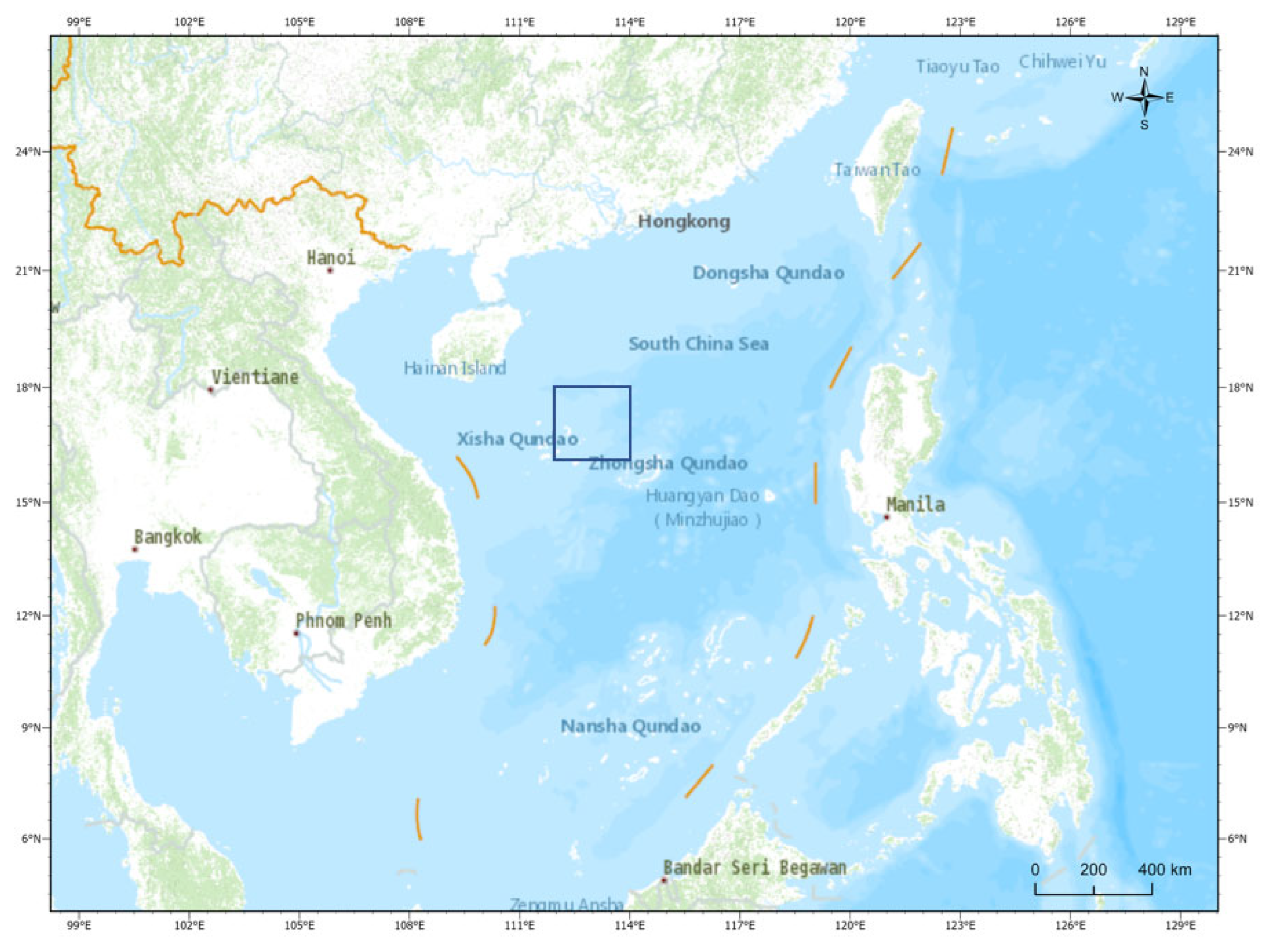
In this study, the seabed topography setting does not utilize the three-dimensional seabed environment model established by QI [27], but introduces the real data from the ETOPO1 [28] dataset to bridge the gap between the simulation environment and actual application scenarios, thereby enhancing the reliability of the simulation environment and providing real data support for the path planning algorithm. In this paper, we take part of the South China Sea as the research object (112° E to 114° E, 16° N to 18° N), as shown in Figure 2.

The ocean current exerts the most significant influence on the optimal path planning for AUV energy consumption. In an ocean current environment, countercurrents directly reduce the navigation speed of AUVs, increase navigation time, increase energy consumption, and potentially threaten navigation safety. Conversely, favorable currents can enhance the velocity of AUVs and conserve a considerable quantity of energy.

The ocean current model in this study is based on the assumption made by Garau that the currents surrounding the AUV are the result of Lamb eddies of unknown position, radius, and strength [29]. He constructed the Navier–Stokes Equations, which describe ocean dynamics, as a combination of single-point Lamb eddies, called viscous Lamb eddies. These equations are designated as follows:

$$\left\{\begin{array}{l}{V}_x(r)=-\lambda \cdot {\displaystyle \frac{y-y_0}{2\pi (r-r_0)}}\cdot \left[1-{\mathrm{e}}^{-{({\displaystyle \frac{r-r_0}{\xi }})}^2}\right]\\ V_y(r)=\lambda \cdot {\displaystyle \frac{x-x_0}{2\pi (r-r_0)}}\cdot \left[1-{\mathrm{e}}^{-{({\displaystyle \frac{r-r_0}{\xi }})}^2}\right]\\ \omega (r)={\displaystyle \frac{\lambda }{\pi {\xi }^2}}{e}^{-{({\displaystyle \frac{r-r_0}{\xi }})}^2}\end{array}\right.$$

(1)

where $V_x\left(r\right), V_y\left(r\right), \omega \left(r\right)$ are the eddy velocity components in the horizontal transverse, horizontal longitudinal, and vertical directions, respectively, and λ, ξ, and $r_0$ are the coordinates of eddy strength, eddy radius, and eddy center position, respectively.

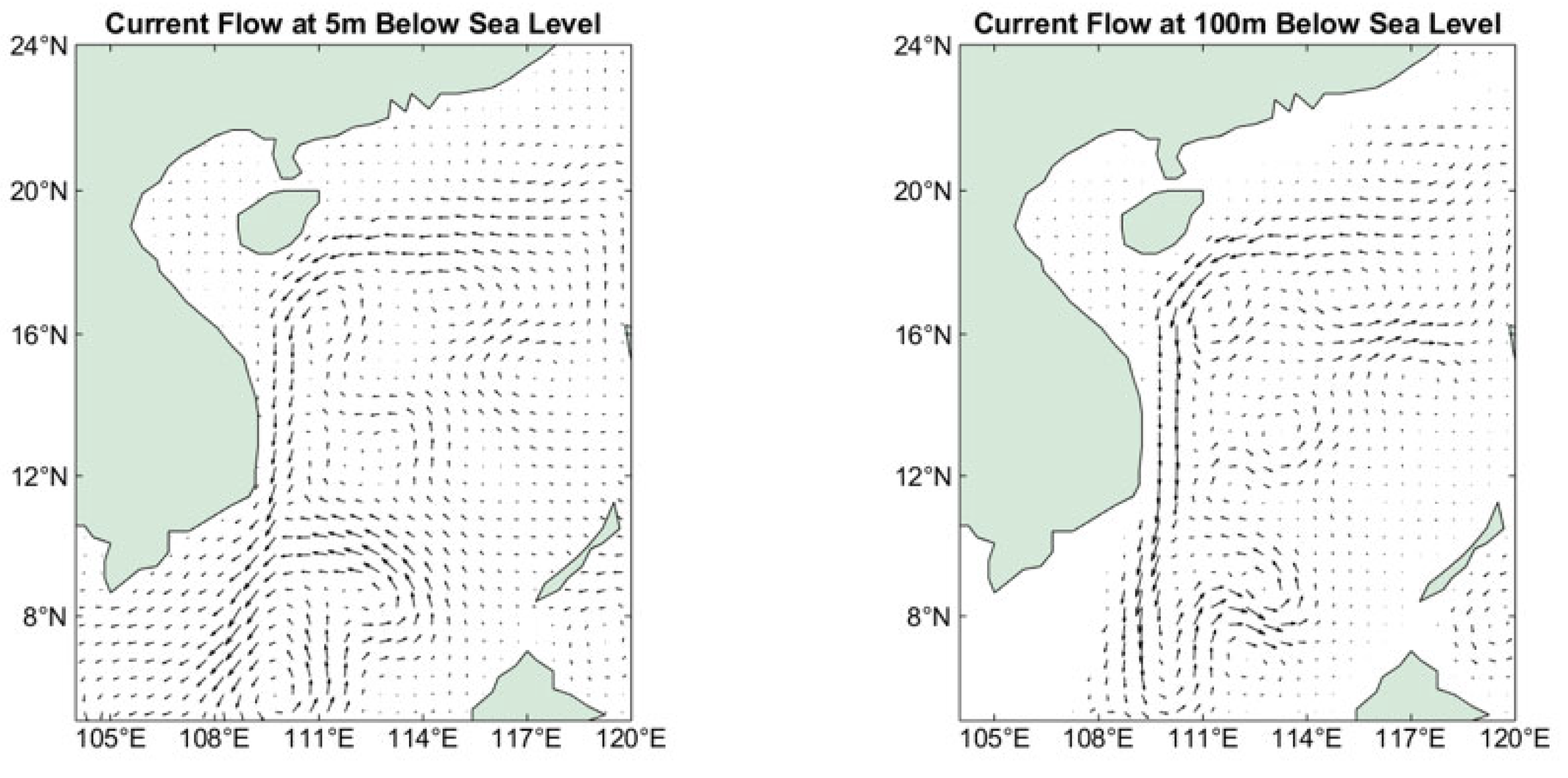
In this paper, based on the data in the SODA [30] dataset, the current field at different depths at a certain moment in the South China Sea region is obtained, as shown in Figure 3. In this study, the parameters of the eddy field will be set according to the data in the dataset in order to simulate the actual ocean currents.

Due to the low velocity of the current in the vertical direction, the effect of the vertical component of the current is disregarded in this paper. Instead, the current is considered to be stratified and stabilized in three-dimensional space as the AUV performs its mission.

In the environment model established in this paper, randomly distributed spherical obstacles are also introduced to increase the realism of the simulation scenario. The size, distributed number, and specific location of these obstacles are randomly generated to simulate various potential obstacles in the ocean, in addition to the terrain. This ensures that the AUV can operate stably in the complex and changing ocean environment. We construct the following mathematical model to describe the randomly distributed obstacles: let the ocean environment be represented by a three-dimensional spatial region $\mathsf{\Omega }\subseteq {ℝ}^3$, and let us consider a set of spherical obstacles, ${\left\{O_i\right\}}_{i=1}^N$, distributed in this environment, where N denotes the total number of obstacles. Each obstacle, $O_i$, is defined as a sphere as follows:

$$O_i:=\{O\in {ℝ}^3:{‖O-c_i‖}_2\le R_i\}$$

(2)

where $c_i=\left(o_{ix}, o_{iy}, o_{iz}\right)$ represents the center position of the obstacle and $R_i$ denotes its radius. The overall underwater three-dimensional environment model is shown in Figure 4. In the figure, the blue spheres represent the obstacles.

2.3. Constraints

The feasibility of a path is determined by the constraints imposed on the AUV. These constraints include several performance constraints, environmental constraints, and synergy constraints. The following constraints are the primary focus of this study.

Terrain and obstacle limitations. The premise of path planning is to find a safe and collision-free path. In this study, the following restrictions are imposed on particle positions, and the corresponding penalty functions are established, which will be presented in Section 4.

$$\left\{\begin{array}{l}\mathrm{Dis}(p_i,c_i)>R_i+d_{safe}\\ z_i>Z_{seabed}+Z_{safe}\end{array}\right.$$

(3)

AUV speed limitation. The localization system of the Stingray II AUV is based on a Kalman filter, with the localization error of the basic localization mode being no greater than 5% at an AUV surge speed of 0.3~2 m/s. Due to the limitations of the stability control system, this paper proposes the following speed limitations for the AUV:

$$v\ge v_{min}=0.3 \mathrm{m}/\mathrm{s}$$

(4)

Ocean current constraints: In this paper, ocean currents are utilized or circumvented by decomposing the vector flow field. Currents that flow outside the designated range are treated as obstacles, and AUVs navigate only within the following current fields:

$$\left\{\begin{array}{l}-0.5 \mathrm{m}/\mathrm{s}\le {\nu }_c\cos \theta \le 0.5 \mathrm{m}/\mathrm{s}\hfill \\ \left|{\nu }_c\sin \theta \right|\le 1 \mathrm{m}/\mathrm{s}\hfill \end{array}\right.$$

(5)

Other limitations: In this study, the speed of the AUV in different path segments is determined according to the travel time, current distribution, and ascent angle. To ensure the safety of the AUV, the vertical thruster is programmed to limit both the ascent and descent speed of the AUV, as follows:

$$\left|v_h\right|\le 0.5 \mathrm{m}/\mathrm{s}$$

(6)

On this basis, a B-spline curve is used to curve-fit the paths to ensure the smoothness of the path transitions.

3. Methodology

3.1. Path Planning Problem Description

The optimal path, $Path=\left\{p_1, p_2, \dots , p_n\right\}$, can be the shortest path in terms of distance traveled, the shortest path in terms of navigation time, or the optimal path in terms of energy consumption. The coordinates of each path waypoint are as follows: $p_i=\left(x_i, y_i, z_i\right)$. Path planning can be described as follows:

$$Path=\min J$$

(7)

$$s.t.\left\{\begin{array}{l}{p}_1=p_{start}\hfill \\ p_n=p_{end}\hfill \\ p_i\notin \left\{O\right\} , \forall i\in \left[1,n\right]\hfill \\ z_i>Z_{seabed} , \forall i\in \left[1,n\right]\hfill \end{array}\right.$$

(8)

where $J$ is the objective function, which represents the goal of path planning, $\left\{O\right\}$ is a set of obstacles, and $Z_{seabed}$ represents the depth of the seabed that corresponds to $p_i$. The process of path optimization is the process of finding the minimum value of the objective function. In order to facilitate the calculation, this study employs a simplified strategy by considering the AUV as a prime model, representing its motion by position changes in three-dimensional space.

To facilitate an understanding of the technical content in this section, a nomenclature table is provided below to define key symbols and terms used in the description of the energy-optimized particle swarm optimization (EOPSO) algorithm and the associated path planning optimization problem. The nomenclature used in this study is summarized in

Table 1. Nomenclature.

Name	Description	Name	Description
$A, v, \rho$	Parameters for the calculation of resistance	$Tmax$	Maximum time limit for travel
$c_1{c}_2$	Learning factor of PSO algorithm	$O\left(X_i\right), H\left(X_i\right)$	Threat functions of terrain and obstacles
$C_d$	Resistance (drag) coefficient of the AUV	$O_i$	Spherical obstacles in ${ℝ}^3$
$d_{safe}$	Safe distance from obstacles	$p_n$	Coordinate of the nth waypoint
$E_{total}$	Total energy consumption of AUV	$P_i$	Power of the ith set of thrusters
$F$	Fitness function	$p_{best}$	Individual best of the particle swarm
$f$	Calculation factor for inertia weights	${ℝ}^3$	Three-dimensional space for path planning
$g_{best}$	Global best of the particle swarm	$R_i$	Radius of the ith obstacles
$k_i$	Thruster power calculation factor	$V_i$	Velocity of the ith particle in the swarm
$L$	Length of a segment of a path	$v_g$	Vehicle speed to ground
$\lambda , \mathsf{\xi }, {\mathrm{r}}_0$	Parameters of the Lamb vortex model	$\omega , {\omega }_{\max }, {\omega }_{\min }$	Inertia weights of PSO algorithm
$m, d$	Population size of the particle swarm	$X_i$	Position of the ith particle in the swarm
$\alpha , \beta$	Factors of the threat function	$Z_{safe}$	Safe height from the seabed

.

3.2. PSO Algorithm

The particle swarm optimization (PSO) algorithm is a population-based heuristic optimization algorithm [31]. In the PSO algorithm, each particle represents a potential solution, and by iterating continuously, the particles keep searching in the solution space. The particle has two main parameters, position $X_i=\left[x_{i1}, x_{i2 }, \dots , x_{id}\right]$ and velocity $V_i=\left[v_{i1}, v_{i2}, \dots , v_{id}\right]$. During the iteration process, the particle adjusts its velocity and position by the best position in its personal experience (individual cognitive part $p_{best}$) and the best position in the whole group (social cognitive part $g_{best}$), which is described as follows in Equation (9):

$$\left\{\begin{array}{l}{v}_i(t+1)=w{v}_i(t)+c_1{r}_1(p_{bes{t}_i}(t)-x_i(t))+c_2{r}_2(g_{best}(t)-x_i(t))\\ x_i(t+1)=x_i(t)+{\nu }_i(t+1)\end{array}\right.$$

(9)

where $\omega$ is the inertia weight, which describes the extent of inheritance of the particle velocity from the previous moment, $c_1, c_2$ are learning factors, $p_{bes{t}_i}\left(t\right)$ and $g_{best}\left(t\right)$ are the individual optimal position and the global optimal position at the time of t iterations, respectively, and $r_1, r_2$ are the random numbers.

The velocity update formula consists of three parts, the first part is the inertia part, that is, the tendency of the particle to continue to move in the direction of the previous velocity, the second part is the individual cognition, which causes the particle to move in the direction of the optimal position that occurs in the iterative process of the particle, that is, it guides the particle to the individual cognitively optimal solution, and the third part is the social cognition, which causes the particle to move toward the optimal position of the group.

After each position update, the fitness value of each particle is recalculated and compared with the value that corresponds to the previous iteration, and $p_{best}$ and $g_{best}$ are determined based on the fitness of the particle, $F\left(x_i\right)$, and its previous best fitness, $F\left(p_{bes{t}_i}\right)$, as follows:

$$p_{bes{t}_i}(t+1)=\left\{\begin{array}{c}{p}_{bes{t}_i}(t), F\left(p_{bes{t}_i}(t)\right)\le F(x_i(t+1))\\ x_i(t+1), F\left(p_{bes{t}_i}(t)\right)>F(x_i(t+1))\end{array}\right.$$

(10)

$$g_{best}(t+1)=\left\{\begin{array}{l}{g}_{best}(t), F(g_{best}(t))\le F(p_{bes{t}_i}(t+1))\hfill \\ p_{bes{t}_i}(t+1), F(g_{best}(t))>F(p_{bes{t}_i}(t+1))\hfill \end{array}\right.$$

(11)

In the particle swarm optimization algorithm path planning, m is the number of particles, which represents the total number of path solutions, and d is the dimension of each particle, which represents the number of intermediate path points on each path. In PSO algorithms, these parameters, as well as the inertia coefficient, ω, and the learning rate, ${\mathrm{c}}_1$, ${\mathrm{c}}_2$, are usually fixed values, but this will result in the range of particles explored being kept constant throughout the algorithm iterations, which could lead to the path planning becoming trapped at a local minimum or result in the convergence of the path planning at a later stage that is not sufficiently rapid.

3.3. AUV Energy-Consumption Modeling

In the study of energy-optimal path planning for AUVs, the construction of an energy model is a key factor in evaluating and optimizing the efficiency of the path, and this section describes the mathematical model used to compute the energy consumption of an AUV through the identified path.

The energy consumption of an AUV is mainly determined by its propulsion system, in this study, the energy consumption of on-board sensors will be ignored, and only the energy consumption model of the six propellers of the AUV will be considered. The drag force acting on the AUV is balanced with the thrust generated by the propellers in the case of uniform speed motion. In this study, the six thrusters of the AUV are categorized into three groups, including the two main thrusters, which provide forward and steering power, with a total power of $P_1$, the lateral thruster, which provides resistance to the lateral currents, with a power of $P_2$, and the three drogue thrusters, which control the lifting and sinking motions, with a total power of $P_3$. The total global energy consumption is defined as follows:

$$E_{total}={\displaystyle \sum _{i=1}^3{\displaystyle {\int }_{t_0}^{t_f}{P}_i}}(t)dt$$

(12)

Based on the formula for the resistance to motion of an underwater robot, the power of the thruster can be deduced as follows [32]:

$$P_i(v)={\displaystyle \frac{1}{\eta }}({\displaystyle \frac{1}{2}}\rho C_{d}A{v}^3)$$

(13)

where $\eta$ is the efficiency of the propulsion system, $C_d$ is the drag coefficient, which depends on the shape and surface properties of the AUV, $A$ is the AUV cross-sectional area, $v$ is the surge speed of the AUV, and $\rho$ is the fluid density.

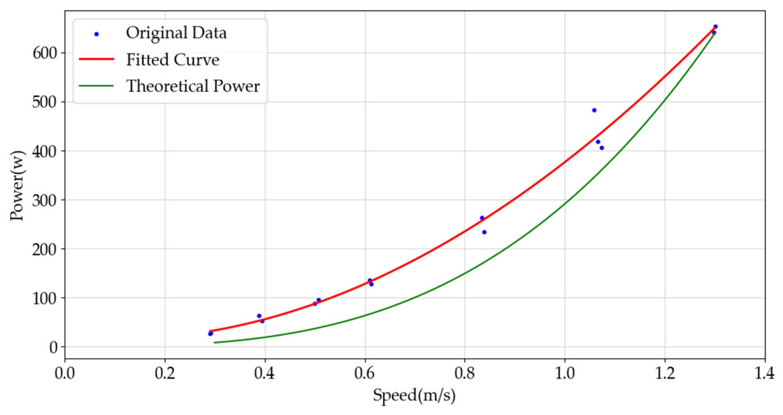
The Stingray II AUV is calculated according to the length of 2 m, width of 1 m, and height of 0.5 m for its area, which faces the current in all directions. In this study, the main thrusters are the main source of energy consumption for the AUV. Experiments on the relationship between main thrusters’ power and surge speed were conducted in a hydrostatic environment, and since the thruster power is cubically related to the speed, this paper fits the experimental results with a cubic curve. A comparison of the actual power of the AUV main thruster obtained and the theoretical power in the ideal case is shown in Figure 5.

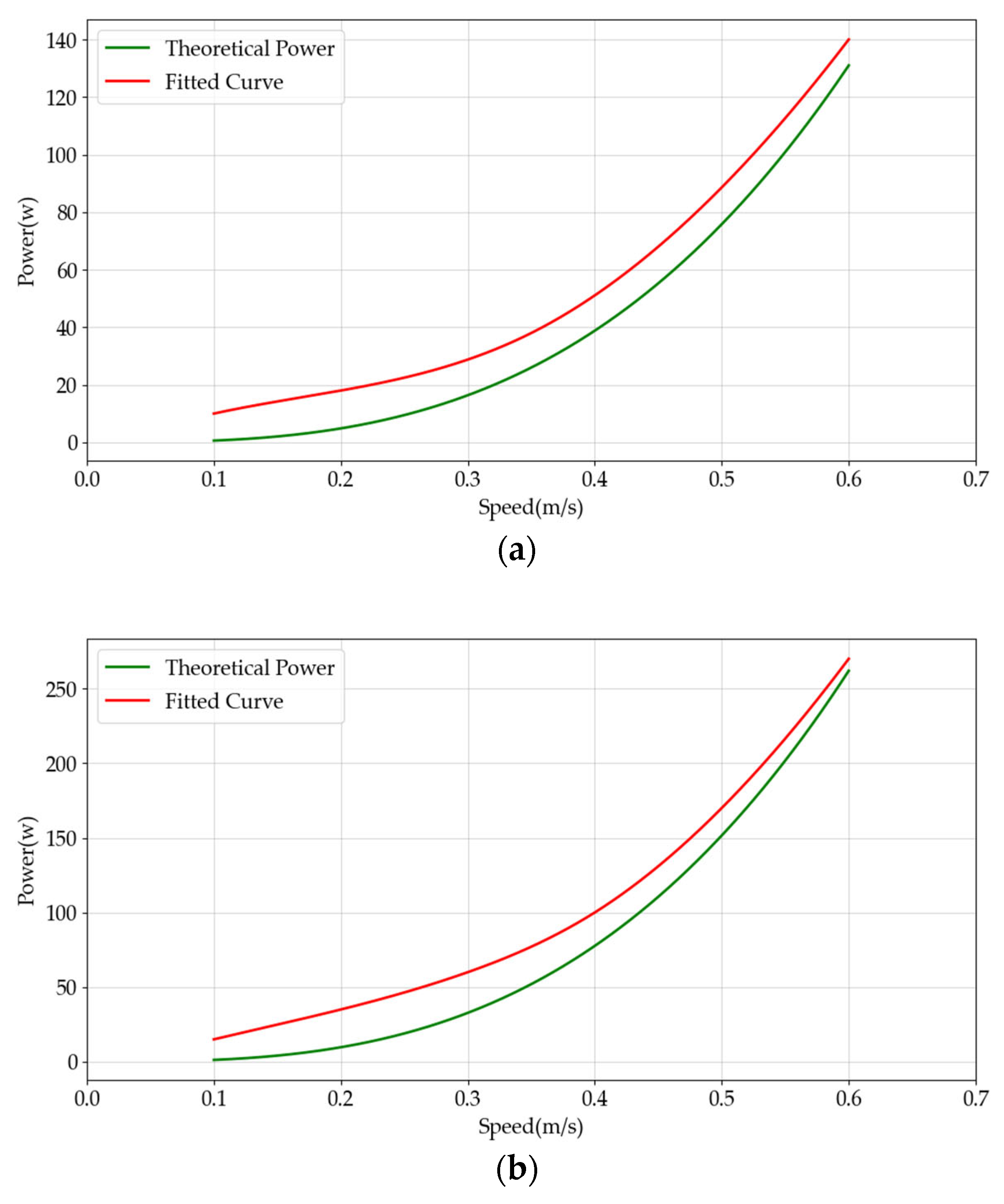
In addition, we experimentally tested the power–velocity model for the lateral and vertical thrusters. The results are shown in Figure 6.

In this study, by default, the bow direction of the AUV is aligned with the direction of the path segment, and the pitch angle is kept at 0. In this kind of motion, the lateral thrusters are solely used to resist the lateral component of the ocean currents on the AUV, while the vertical thrusters are solely used to control the rising and sinking motions of the AUV, and the effect of coupling between the thrusters on the motion of the AUV is not taken into account.

In addition, the component of the ocean current in the vertical direction is considered to be negligible and is therefore not included in the analysis. The actual speed at which an AUV navigates a section of its path under the influence of currents is not the surge speed. The actual velocity of AUV is denoted as $v_g$, which represents the velocity of AUV to the ground and can be calculated as follows:

$$v_g=v+{\displaystyle \frac{v_c\cdot \overrightarrow{p_{\iota }{p}_{\iota +1}}}{‖\overrightarrow{p_{\iota }{p}_{\iota +1}}‖}}$$

(14)

where $v$ represents the surge speed of the AUV and $v_c$ represents the velocity of the ocean current, whose component in the direction of the velocity of AUV affects the actual travel speed.

3.4. Optimal Speed Calculation with the T_max Limit

When an AUV performs a certain task, it is often subject to a maximum time limit, which makes it necessary to consider the travel time constraint when considering energy-optimal path planning, rather than just considering energy consumption without considering the final elapsed time. However, existing three-dimensional path planning for AUVs that considers a travel time constraint is limited to path planning at fixed speeds [33,34]. In this paper, we argue that for a given path, assigning and optimizing AUV travel speeds for different path segments within $T_{max}$ constraints can help save a lot of energy.

In this regard, this paper assumes a maximum travel time $T_{max}$ for the mission and thereby simplifies the problem to an AUV energy consumption optimization problem under the influence of a two-dimensional current field. In this paper, the speed at which the AUV consumes the least energy per unit of distance traveled is defined as the optimal speed, $v_b$, of the path segment, and the optimal speed of the AUV that passes through a segment of the same path is different in different ocean current fields.

$$v_b=\arg {\min }_v{E}_{total}$$

(15)

Assume that for a section of path of length L, the AUV passes through this section of path with a certain surge velocity, v. The distribution within this section of path is a constant flow field, the velocity of the current is $v_c$, and the velocity of the AUV makes an angle with the velocity of the current of $\theta$. Then, the velocity of the AUV relative to the ground at this point, $v_g$, and the sideways velocity, $v_{side}$, which the AUV must resist, are expressed as follows:

$$\left\{\begin{array}{l}{v}_g=v+v_c\cos \theta \\ v_{side}=v_c\sin \theta \end{array}\right.$$

(16)

The time required to pass along this path segment is expressed as follows:

$$t={\displaystyle \frac{L}{v+v_c\cos \theta }}$$

(17)

The power of the AUV thrusters is simplified as follows:

$$\left\{\begin{array}{l}{P}_1=k_1{v}^3\\ P_2=k_2{(v_c\sin \theta )}^3\end{array}\right.$$

(18)

where $k_1$ and $k_2$ are the power calculation coefficients for the main and lateral thrusters, respectively, which are kept constant in a stable environment. Then, the total energy consumption of the AUV can be derived as follows:

$$E_{total}=\int (P_1+P_2)dt=\int (k_1{v}^3+k_2{(v_c\sin \theta )}^3)dt$$

(19)

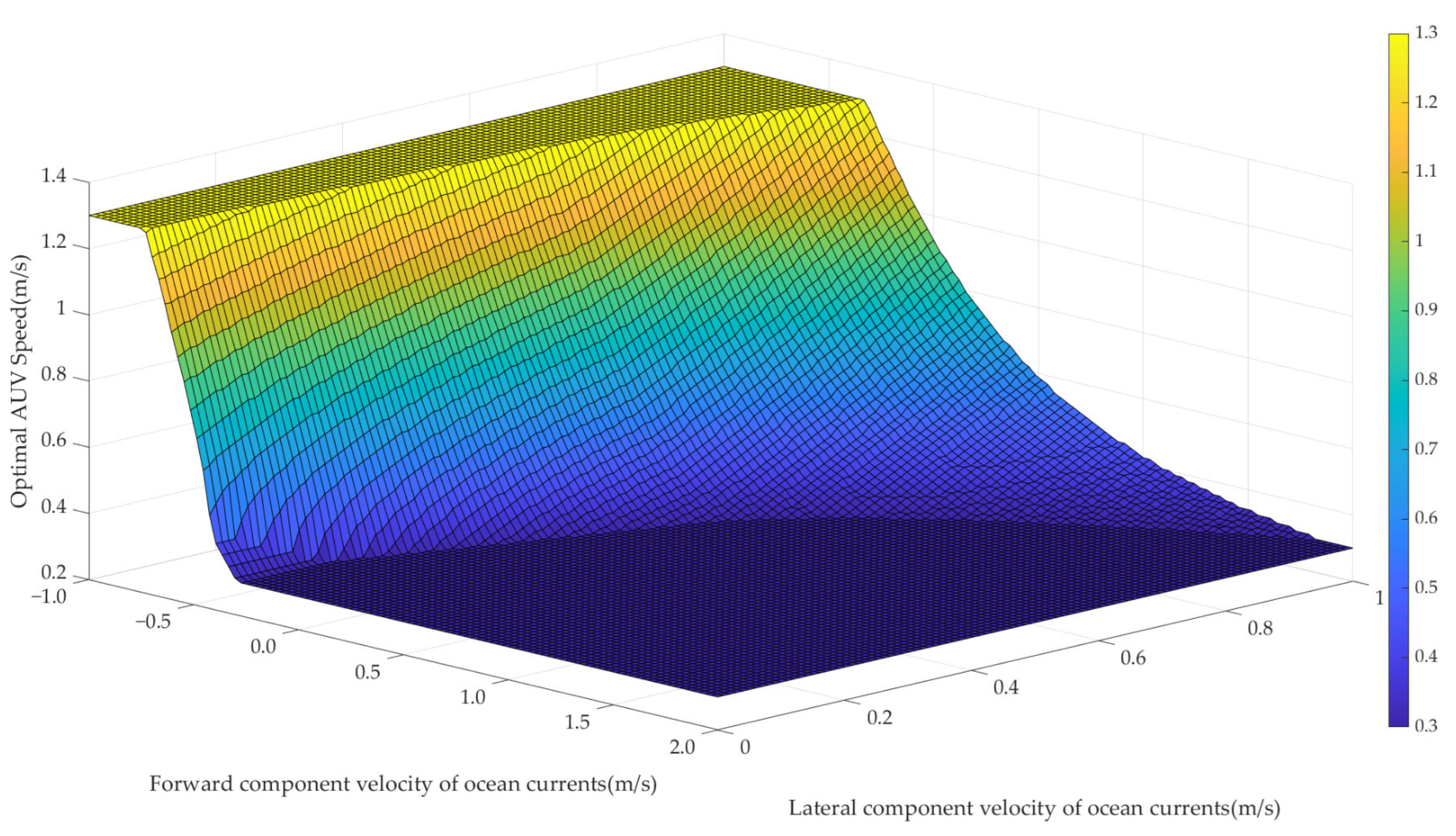
The ocean current model is decomposed into forward and lateral components, both of which are relative to the AUV’s velocity. We analyzed the optimal AUV speed for forward current components ranging from −1 m/s to 2 m/s and lateral components ranging from 0 to 1 m/s. The resulting optimal AUV speeds under varying current conditions are presented in Figure 7.

The subsequent analysis considers the optimal speed of the AUV under the influence of three-dimensional stratified ocean currents. In three-dimensional path planning, the partial velocity, $v_h$, of the AUV in the vertical direction is determined by $v_g$, as follows:

$$v_h={\displaystyle \frac{\mathsf{\Delta }h}{t}}={\displaystyle \frac{\mathsf{\Delta }h(v+v_c\cos \theta )}{L}}$$

(20)

where $\Delta h$ is the projection of $\overrightarrow{p_i{p}_{i+1}}$ onto the Z axis. If the derived $v_h$ exceeds the limit, the path cannot be generated. This study ignores changes in seawater density within a certain range. Additionally, the AUV is assumed to be neutrally buoyant in the water, and the energy consumption generated by the vertical thruster for its motion in a constant depth state is neglected. Similarly, the energy consumption of the AUV vertical thruster can be obtained as follows:

$$P_3=k_3{({\displaystyle \frac{\mathsf{\Delta }h(v+v_c\cos \theta )}{L}})}^3$$

(21)

where $k_3$ is the power coefficient of the vertical thruster. Then, the total energy consumption of the AUV at this point is shown below:

$$E_{total}={\displaystyle \int \left(k_1{v}^3+k_2{(v_c\sin \theta )}^3+k_3{(\frac{\Delta h(v+v_c\cos \theta )}{L})}^3\right)}dt$$

(22)

The qualification, $T_{max}$, is added as follows:

$${\displaystyle \frac{L}{v+v_c\cos \theta }}\le T_{max}$$

(23)

In this study, the Sequential Quadratic Programming (SQP) algorithm is used to solve this nonlinear optimization problem. The SQP algorithm solves the nonlinear optimization problem by converting it into a series of quadratic programming subproblems, each of which approximates the original problem but is easier to solve [35]. In this paper, we place the computation of fitness value in the SQP algorithm, which will be used to find the optimal speed of each path segment with minimal energy consumption, as shown in Algorithm 1.

Algorithm 1 EOPSO Algorithm for AUV Path Planning

STEP 1: Create a 3D environmental model that includes seafloor topography, static obstacles, and ocean currents. STEP 2: Initial particle paths $\left\{p_1, p_2, \dots , p_n\right\}$, maximum iterations I, learning factors, inertia weight, and other parameters. STEP 3: Initial parameters of the SQP algorithm, including the velocity, ${\mathit{v}}_j$, tolerance, tol, step size, ${\alpha }_0$, maximum iterations N, and Tmax. STEP 4: Repeat       for each i          Compute the value of the energy function according to Equation (22) at ${\mathit{v}}_j$.          Compute the gradient of Etotal at ${\mathit{v}}_j$.          Update the particle velocities and positions and avoid collisions using Equation (9).          Repeat            Compute the Hessian according to HEtotal at ${\mathit{v}}_j$.            ${\mathit{H}}_{E_{\mathrm{total}}}\left({\mathit{v}}_j\right)=\left[\begin{array}{cccc}{\displaystyle \frac{{\partial }^2{E}_{\mathrm{total}}}{\partial {\mathit{v}}_{j1}^2}}& {\displaystyle \frac{{\partial }^2{E}_{\mathrm{total}}}{\partial {\mathit{v}}_{j1}\partial {\mathit{v}}_{j2}}}& \dots & {\displaystyle \frac{{\partial }^2{E}_{\mathrm{total}}}{\partial {\mathit{v}}_{j1}\partial {\mathit{v}}_{jN}}}\\ {\displaystyle \frac{{\partial }^2{E}_{\mathrm{total}}}{\partial {\mathit{v}}_{j2}\partial {\mathit{v}}_{j1}}}& {\displaystyle \frac{{\partial }^2{E}_{\mathrm{total}}}{\partial {\mathit{v}}_{j2}^2}}& \dots & {\displaystyle \frac{{\partial }^2{E}_{\mathrm{total}}}{\partial {\mathit{v}}_{j2}\partial {\mathit{v}}_{jN}}}\\ ⋮& ⋮& \ddots & ⋮\\ {\displaystyle \frac{{\partial }^2{E}_{\mathrm{total}}}{\partial {\mathit{v}}_{jN}\partial {\mathit{v}}_{j1}}}& {\displaystyle \frac{{\partial }^2{E}_{\mathrm{total}}}{\partial {\mathit{v}}_{jN}\partial {\mathit{v}}_{j2}}}& \dots & {\displaystyle \frac{{\partial }^2{E}_{\mathrm{total}}}{\partial {\mathit{v}}_{jN}^2}}\end{array}\right]$                          (24)            Solve the QP subproblem to find the search direction as follows:            $\underset{\mathsf{\Delta }\mathit{v}}{\min }\left[\nabla f{({\mathit{v}}_j)}^T\mathsf{\Delta }\mathit{v}+{\displaystyle \frac{1}{2}}\mathsf{\Delta }{\mathit{v}}^T{\mathit{H}}_j\mathsf{\Delta }\mathit{v}\right]$                                    (25)            Apply the constraints according to Equation (23).            Conduct a line search to determine step size αi            Update ${\mathit{v}}_{j+1}={\mathit{v}}_j+{\alpha }_i\mathsf{\Delta }\mathit{v}$          Until $\parallel \nabla E_{total}\left({\nu }^{\left(i\right)}\right)\parallel <tol \mathrm{or} i\ge N$                                     (26)           ${\mathit{v}}_b={\mathit{v}}_j$          Determine if re-planning is required.     Until $iter\ge I$

STEP 5: Output path and optimal velocity: ${\mathit{v}}_b$ and Etotal.

For a specific path, $\left\{p_1, p_2, \dots , p_n\right\}$, the abovementioned algorithm calculates the optimal speed of each path segment. Thereafter, the energy consumption of each segment of the path is calculated, and the results are summed to obtain the total energy consumption of the entire path, where $f(v_j)$ is the energy consumption function of the AUV, and ${\alpha }_i$ is the step size of the SQP algorithm.

3.5. Fitness Function

The fitness function represents the fundamental element of the PSO algorithm. In path planning problems, the fitness function is typically formulated as the objective of optimization.

The objective of this research is to identify the optimal energy consumption path in a complex three-dimensional environment. The focus of this paper is to optimize the total energy consumption of through-path planning. The fitness function of the PSO algorithm in this paper is constructed based on the energy consumption model established in the previous section, considering other constraints.

The optimal travel speed of the AUV in the current field environment is determined by the energy consumption model of the AUV, which is established in this paper. This model considers the effects of ocean currents, the travel time of the AUV, and the travel distance. The fitness function not only considers the energy consumption of the AUV but also needs to consider the threat of the seabed topography and obstacles to the AUV. In this paper, the fitness function is defined as follows:

$$F(X_i)=E(X_i)+\alpha O(X_i)+\beta H(X_i)$$

(27)

where $E\left(X_i\right)$ is the total energy consumption of the AUV, $O\left(X_i\right)$ denotes the penalty function that corresponds to the minimum safe distance between the path point and the obstacle, α is the weighting coefficient of the safe distance function, $H\left(X_i\right)$ denotes the penalty function that corresponds to the minimum safe distance between the path point and the undersea terrain, and β is its weighting coefficient, which controls the degree of influence of the safe distance of the obstacle in the fitness function. For a specific solution, $X_i$, the function, $O\left(X_i\right)$, of the obstacle threat to the AUV takes the following form:

$$O(X_i)={\displaystyle \sum _{j=1}^N{\displaystyle \sum _{i=1}^{n}O}}(p_i)$$

(28)

$$O(p_i)=\left\{\begin{array}{l}{\displaystyle \frac{1}{dist(p_i,\left\{0_j\right\})+\epsilon }}, dist(p_i,\left\{\begin{array}{c}{0}_j\end{array}\right\})<d_{safe}\hfill \\ 0, dist(p_i,\left\{\begin{array}{c}{0}_j\end{array}\right\})\ge d_{safe}\hfill \end{array}\right.$$

(29)

The form of the function $H\left(X_i\right)$ of the seafloor topography on the AUV threat is as follows:

$$H(X_i)={\displaystyle \sum _{j=1}^d}H(x_{ij})$$

(30)

$$H(x_{ij})=\left\{\begin{array}{l}{\displaystyle \frac{1}{z_j-Z(x_j,y_j)}}, z_j<Z\left(x_j,y_j\right)+Z_{safe}\hfill \\ 0, z_j\ge Z\left(x_j,y_j\right)+Z_{safe}\hfill \end{array}\right.$$

(31)

where n is the number of path segments, d is the number of intermediate path points, and $n=d+1$.

3.6. Improved EOPSO Algorithm

In the particle swarm algorithm, the learning factors, $c_1$ and $c_2$, and the inertia coefficients, $\omega$, in the particle velocity update formula play a crucial role in maintaining a balance between global exploration and the local exploitation of particles.

If the inertia weight, $\omega$, is large, it indicates that the particle has a strong detection ability and is suitable for a large-scale search of the whole planning space. If it is small, it is suitable for small-scale searches of the localized area.

We propose a new method that combines particle positions and randomness to adjust $\omega$, intending to enhance the search capacity of the algorithm while reducing the probability of falling into local minima.

When a particle explores the boundaries of the map, it is possible for the fitness value at the map edge to be less than that within the map, which may result in the velocity of the particle being the same as that which causes the particle to leave the map, thus falling into a local minimum. In this context, during each iteration, we evaluate the location of the optimal particle. If the particle is near the map boundary and the expected next-generation position is beyond it, the inertia weights are inverted, and their absolute value is increased to drive the particle back into the search space.

$${\omega }_{\mathrm{new}}=f\omega , \hspace{1em}f=\left\{\begin{array}{l}-a, \mathrm{if} \mathrm{any} x_{ij}^{t+1}\notin {ℝ}^3\hfill \\ 1, \mathrm{otherwise}\hfill \end{array}\right.$$

(32)

Here, $f$ is an inertia coefficient computation factor, and a is a constant used to increase the absolute value of the inertia weights so that particles are assisted in leaving the map range to enhance particle exploration.

In the typical scenario, the inertia weights exhibit a linear decline as the number of iterations increases. This approach has been demonstrated to enhance the fine-tuning characteristics of the PSO [36], and in agreement with this strategy, the inertia weights are expressed as follows:

$$\omega =f\times ({\omega }_{\max }-({\omega }_{\max }-{\omega }_{\min })\times {\displaystyle \frac{iter}{ma{x}_{iter}}}), \hspace{1em}f=\left\{\begin{array}{l}-a, \mathrm{if} \mathrm{any} x_{ij}^{t+1}\notin {ℝ}^3\hfill \\ 1, \mathrm{otherwise}\hfill \end{array}\right.$$

(33)

Furthermore, during the process of particle iteration, local minima frequently occur, despite the restriction on the position of the particles. Given the constraints imposed by the learning factor and inertia coefficients on the region explored by the algorithm, it is necessary to introduce a re-planning mechanism during iteration. This mechanism must overcome the limitations of the current global and local optimal solutions and facilitate the acquisition of a new population of particles. When the algorithm does not observe a significant improvement in the global optimal solution for several consecutive iteration cycles and the fitness value of the current global optimal solution exceeds the theoretical minimum energy consumption value based on the shortest path computation, a complete re-planning is triggered. At this point, all particles are reset to new random locations within the search space.

The re-planning strategy is shown to be effective if the new global optimal solution shows lower energy consumption than before. The specific steps are represented in Figure 8.

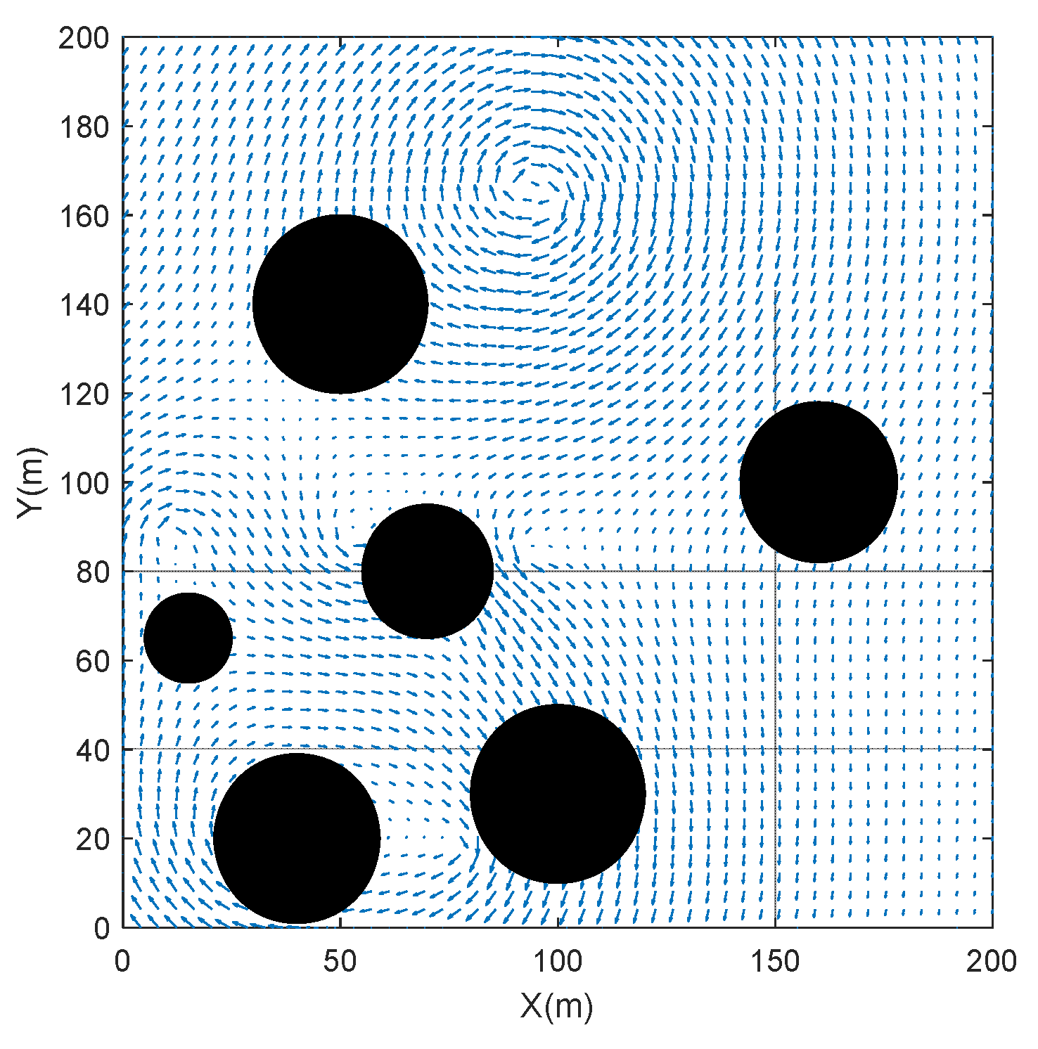
In order to ascertain the efficacy of the proposed re-planning strategy, a series of simulation experiments were conducted in a two-dimensional environment. As depicted in Figure 9, the scenario was set within a 200 m × 200 m plane, where ocean currents and obstacles were distributed. To validate the effectiveness of the re-planning strategy, we designed experiments using two distinct sets of starting and ending points.

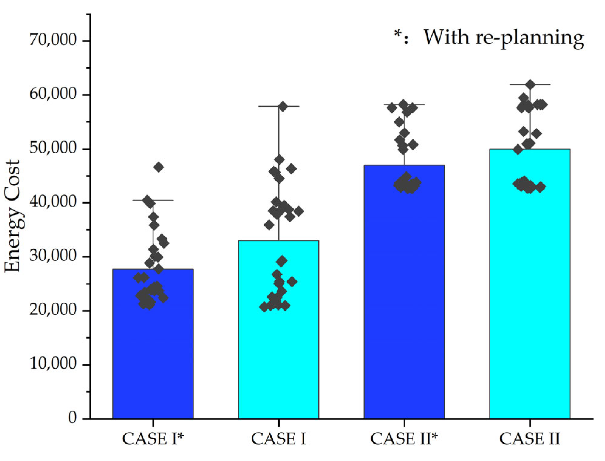
The results of these experiments, presented in Figure 10, demonstrate that the incorporation of a re-planning strategy into a path planning algorithm can effectively reduce the likelihood of the algorithm reaching a local minimum, accelerate the rate of convergence, and enhance the algorithm’s resilience.

4. Results and Discussion

To assess the efficacy of the energy-optimal path planning algorithm proposed in this paper, the simulation results of path planning in different cases are presented and analyzed in this section. The flow field and obstacles are randomly generated, the seafloor topography is derived from real data from a portion of the South China Sea (112° E to 114° E, 16° N to 18° N), and the underwater vehicle is regarded as a mass point.

Simulation experiments were conducted for different starting and ending points to compare the path planning effect of the EOPSO algorithm with the PSO algorithm, GA algorithm, and other algorithms. The computer simulation platform is MATLAB 2020b, the processor is an Intel(R) Core (TM) I7-8700U CPU @ 1.80 GHz 2.00 GHz with 16 GB of RAM, and the operating system is Windows 10, 64-bit.

4.1. Simulation Setup

In this study, three sets of experiments were conducted. A three-dimensional seabed environment model described by an exponential function was used in the first set of experiments. In addition, complex stratified current fields, as well as static obstacles, were incorporated. The parameters that define these components are presented in

Table 2. Simulation conditions for re-planning validation experiments.

Parameter	Value
number of obstacles, N, in Case I	3
number of obstacles, N, in Case II and Case III	2
Parameters of the current field in Case I	$\lambda =1.2, \mathsf{\xi }=500 \mathrm{m}, n=10$
Parameters of the current field in Case II and Case III	$\lambda =1.2, \mathsf{\xi }=100 \mathrm{km}, n=5$
total number of particles	50
number of control points, d	4
maximum number of iterations	200
Parameters of inertia weight	${\omega }_{\max }=0.9, {\omega }_{\min }=0.4$
$\mathrm{learning} \mathrm{rate}, c_1$$, c_2$	$c_1=2.05, c_2=2.05$

.

In order to facilitate a comparison of the performance gap between the algorithms, the following constraints were implemented:

The PSO and GA algorithms are classical shortest-path algorithms. The optimization goal is the length of the path. In this paper, the SQP optimal speed algorithm is combined with these algorithms to find the total energy consumption for comparison. The PSO-TO and GA-TO algorithms are time-optimal path planning algorithms with fixed AUV speeds. In the experiment, the AUV speed was fixed at 0.5 m/s, and the optimization goal was the total travel time. The algorithms utilize favorable currents and avoid unfavorable currents to a certain extent, but their consideration of lateral currents is lacking. This study also implemented the aforementioned enhancements to the QPSO algorithm [37], thereby substantiating the efficacy of the algorithmic improvements.

In addition, we mainly used the following metrics to evaluate the planned paths:

Travel time: AUVs are often time-bound to accomplish their mission, so travel time is an important indicator.

Route length: In this paper, we use uniform gridded coordinates to compare the sum of the lengths of each route.

Time: The time required to generate paths using different algorithms is an important evaluation criterion.

Total energy consumption: The focus of this study is on planning the energy-optimized three-dimensional paths, and this paper will focus on comparing the total energy consumption consumed by AUVs under different conditions with different algorithms.

4.2. CASE I

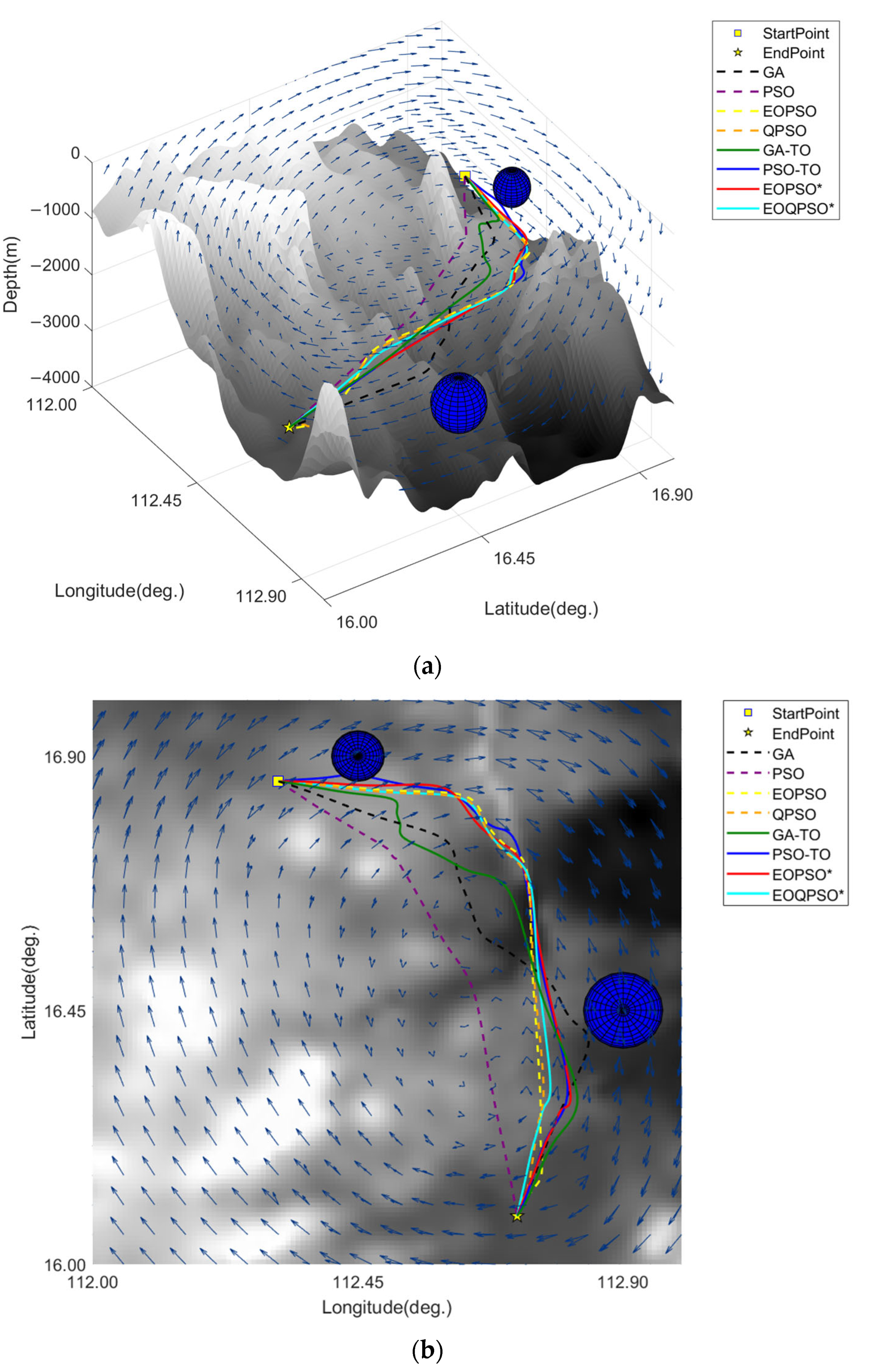
In the first set of experiments, we focus on testing the performance of the algorithms improved in this paper in a small environment that contains complex currents, static obstacles, and undersea terrain. The results of the simulation are shown in Figure 11. In this set of simulations, we deliberately included an obstacle between the start and end points to avoid generating overly simple paths. Due to the complexity of ocean currents, there is a large difference between the optimal and shortest paths. It is worth noting that in this simulation, the paths generated by the EOPSO and EOQPSO algorithms are not similar. The EOPSO algorithm, combined with the re-planning strategy, is able to explore more areas and search well even in small areas.

Table 3. AUV speeds for different path segments.

Algorithm	AUV Travel Speeds(m/s)
	$\overrightarrow{{\mathit{p}}_1{\mathit{p}}_2}$	$\overrightarrow{{\mathit{p}}_2{\mathit{p}}_3}$	$\overrightarrow{{\mathit{p}}_3{\mathit{p}}_4}$	$\overrightarrow{{\mathit{p}}_4{\mathit{p}}_5}$	$\overrightarrow{{\mathit{p}}_5{\mathit{p}}_6}$
① GA	0.30	0.30	0.30	0.33	0.30
② PSO	0.30	0.30	0.30	0.30	0.30
③ EOPSO	0.30	0.30	0.30	0.30	0.30
④ EOQPSO	0.30	0.30	0.30	0.30	0.30
⑤ GA-TO	0.50	0.50	0.50	0.50	0.50
⑥ PSO-TO	0.50	0.50	0.50	0.50	0.50
⑦ EOPSO*	0.56	0.45	0.46	0.48	0.56
⑧ EOQPSO*	0.58	0.45	0.51	0.56	0.57

The asterisk (*) in EOPSO* and EOQPSO* denotes paths generated under a maximum time limit $T_{max}$.

illustrates the sailing speeds achieved by the various algorithms across the different segments of the path. EOPSO* and EOQPSO* denote the result of path planning using the travel time of the PSO-TO algorithm as the maximum time limit, $T_{max}$, parameter of the EOPSO and EOQPSO algorithms, respectively. The AUV demonstrates the greatest energy efficiency by maintaining the lowest constrained speed in situations in which currents have minimal impact on navigation. In contrast, the EOPSO* and EOQPSO* algorithms are capable of assigning optimal speeds to path segments, thereby optimizing the total energy consumed by the AUV when there is a maximum time constraint.

In this study, 30 repetitive experiments were conducted for this case.

Table 4. Comparison of performance metrics of different algorithms in CASE Ι.

Algorithm	Length of Path (m)		Travel Time (s)		Energy Consumption (kJ)		Time (s)
	Mean	Std.	Mean	Std.	Mean	Std.
① GA	1217.5	10.0	3122.5	462.5	257.6	58.6	46.3
② PSO	1191.5	0.5	3071.6	103.2	254.4	10.8	14.5
③ EOPSO	1449.1	59.1	2468.2	148.1	134.0	11.9	347.7
④ EOQPSO	1404.5	74.6	2577.0	172.3	152.0	18.5	366.7
⑤ GA-TO	1245.5	26.7	1858.8	53.4	238.2	9.3	194.6
⑥ PSO-TO	1351.7	76.1	1604.9	57.4	208.7	12.6	416.5
⑦ EOPSO*	1365.2	67.0	1604.9	0.0	191.7	17.4	626.3
⑧ EOQPSO*	1294.6	58.5	1604.9	0.0	229.4	18.7	658.3

The asterisk (*) in EOPSO* and EOQPSO* denotes paths generated under a maximum time limit $T_{max}$.

lists the path performance metrics for different algorithms in the 30 experiments. The EOPSO algorithm is able to save almost half of the energy consumption relative to the GA algorithm combined with the optimal speed algorithm and the PSO without considering the sailing time constraints. A comparison of EOPSO and EOQPSO reveals that the QPSO algorithm does not demonstrate a superior convergence capability or computational speed when used in conjunction with the SQP algorithm to determine the optimal speed. A comparison of the last four sets of results reveals that following the introduction of a maximum sailing time limit, EOPSO is capable of further optimizing energy consumption through the application of the PSO-TO algorithm. However, a notable decline in energy efficiency is observed in EOQPSO relative to PSO-TO.

The objective of this experimental investigation was to ascertain the efficacy of the EOPSO algorithm in a simulation environment. The findings indicate that the algorithm is capable of identifying a more energy-efficient path through a complex ocean current field, while also reducing the computation time relative to the QPSO algorithm. This is due to the fact that the incorporation of the SQP algorithm effectively increases the constraints of the problem, which, in turn, significantly reduces the feasible solution space of the problem. The QPSO is more inclined toward global search, whereas the SQP is a local optimization process. The addition of sailing time constraints makes it more challenging for the QPSO to be confined to a limited feasible solution space. In the case of the PSO, the velocity update serves to guide the particles toward a gradual convergence, and in a smaller solution space, it may be more efficient to tune to solutions that satisfy the time constraints.

4.3. CASE II

For the second set of experiments, the results are shown in Figure 12. From the top view, it can be observed that the paths planned by the GA and PSO algorithms exhibit minimal influence of the ocean current on the AUV travel speed. However, the AUV is more susceptible to the lateral component of the ocean current. In contrast, the path planned by the EOPSO algorithm predominantly follows the downstream direction, aligning closely with the direction of the ocean current. This configuration enhances the surge speed and conserves energy, while the lateral component of the ocean current is comparatively smaller, providing the AUV with a certain degree of stability. The lateral component of the current is smaller in this path, which has the effect of improving the controllability and safety of the AUV to a certain extent.

Table 5. AUV speeds for different path segments.

Algorithm	AUV Travel Speeds (m/s)
	$\overrightarrow{{\mathit{p}}_1{\mathit{p}}_2}$	$\overrightarrow{{\mathit{p}}_2{\mathit{p}}_3}$	$\overrightarrow{{\mathit{p}}_3{\mathit{p}}_4}$	$\overrightarrow{{\mathit{p}}_4{\mathit{p}}_5}$	$\overrightarrow{{\mathit{p}}_5{\mathit{p}}_6}$
① GA	0.30	0.30	0.30	0.33	0.30
② PSO	0.30	0.30	0.30	0.30	0.30
③ EOPSO	0.30	0.30	0.30	0.30	0.30
④ EOQPSO	0.30	0.30	0.30	0.30	0.30
⑤ GA-TO	0.50	0.50	0.50	0.50	0.50
⑥ PSO-TO	0.50	0.50	0.50	0.50	0.50
⑦ EOPSO*	0.41	0.39	0.39	0.69	0.66
⑧ EOQPSO*	0.40	0.39	0.40	0.69	0.65

The asterisk (*) in EOPSO* and EOQPSO* denotes paths generated under a maximum time limit $T_{max}$.

shows the surge speeds of different algorithms for each segment of the path. Comparing algorithms ①, ②, ③, and ④, it can be seen that the optimal speed of AUV, calculated by the SQP algorithm, is mostly equal to the minimum speed, $v_{min}$, without time constraints, which is because, in the case of non-countercurrent and small lateral components of the ocean current, the energy consumption per unit length to maintain the minimum speed is minimized. Compared with algorithms ⑤, ⑥, ⑦, and ⑧, the optimal speed of each section of the path solved by the SQP algorithm is not the same after taking the time calculated by the PSO-TO algorithm as a constraint, $T_{max}$, which is the result of the combination of several factors. In this scenario, the results of EOPSO and EOQPSO are similar in all aspects, including the generated paths and the computed optimal speeds.

In this study, 30 repetitive experiments were conducted for this case.

Table 6. Comparison of performance metrics of different algorithms in CASE ΙI.

Algorithm	Length of Path (km)		Travel Time (h)		Energy Consumption (kJ)		Time (s)
	Mean	Std.	Mean	Std.	Mean	Std.
① GA	215.5	7.4	186.6	6.2	57,209.7	4432.0	107.4
② PSO	203.4	0.4	181.5	1.2	46,086.9	550.6	17.1
③ EOPSO	274.6	4.0	153.1	5.7	38,489.6	203.5	368.9
④ EOQPSO	270.5	2.9	150.3	2.0	38,850.4	433.2	372.3
⑤ GA-TO	232.7	11.5	109.5	3.9	58,815.9	3825.4	240.8
⑥ PSO-TO	267.2	2.0	100.4	0.2	48,776.8	572.1	371.2
⑦ EOPSO*	271.8	3.6	100.4	0.0	44,801.2	134.7	743.4
⑧ EOQPSO*	265.6	1.8	100.4	0.0	45,063.6	359.4	738.3

The asterisk (*) in EOPSO* and EOQPSO* denotes paths generated under a maximum time limit $T_{max}$.

lists the path performance metrics for different algorithms in the 30 experiments. Firstly, a comparison of the EOPSO algorithm proposed in this paper with the GA and PSO algorithms, which combine the optimal speed algorithm without considering travel time constraints, reveals that the EOPSO algorithm can save 30% and 16% of energy consumption relative to the GA and PSO algorithms, respectively. Furthermore, they save more than 15% of energy consumption, even though the planned paths are slightly longer than those of the remaining two algorithms. This is due to the utilization of favorable ocean currents. Under the $T_{max}$ limitation, the paths planned by EOPSO can save 10% energy consumption compared to the PSO-TO algorithm. This is achieved while maintaining the same travel time or even reducing it. Furthermore, the improved EOPSO algorithm demonstrates enhanced robustness. It is noteworthy that the energy optimization and robustness of the EOPSO algorithm are, on average, slightly superior to those of the EOQPSO algorithm.

This experiment also better verifies that ocean currents play an important role in AUV path planning, and the rational use of ocean currents can effectively shorten missions and save energy.

4.4. CASE III

To further validate the utility of the EOPSO algorithm, we interchanged the starting and ending points and conducted another set of experiments.

A comparison of the path planning results from each algorithm is shown in Figure 13. As illustrated by the three-dimensional graphs, a portion of the path segments planned for the AUV by the GA and PSO algorithms are in opposition to the current, resulting in a slight increase in the overall travel time and energy consumption of CASE II compared to CASE I. The improved EOPSO algorithm demonstrates efficacy in identifying optimal paths that traverse the middle of the complex seabed topography. Furthermore, the planned paths align with the downstream current, providing compelling evidence of the algorithm’s effectiveness. This substantiates the practicality of the algorithm. Given that the optimal path traverses a region with complex terrain, the traditional PSO and GA algorithms are prone to premature convergence or local minima. In contrast, the improved EOPSO algorithm in this paper employs a re-planning mechanism that enhances the avoidance of local minima and facilitates the exploration of a more extensive range of potential regions on the map.

Similarly,

Table 7. AUV speeds for different path segments in CASE ΙΙI.

Algorithm	AUV Travel Speeds (m/s)
	$\overrightarrow{{\mathit{p}}_1{\mathit{p}}_2}$	$\overrightarrow{{\mathit{p}}_2{\mathit{p}}_3}$	$\overrightarrow{{\mathit{p}}_3{\mathit{p}}_4}$	$\overrightarrow{{\mathit{p}}_4{\mathit{p}}_5}$	$\overrightarrow{{\mathit{p}}_5{\mathit{p}}_6}$
① GA	0.30	0.30	0.30	0.30	0.31
② PSO	0.30	0.30	0.30	0.30	0.30
③ EOPSO	0.30	0.30	0.30	0.30	0.30
④ EOQPSO	0.30	0.30	0.30	0.30	0.30
⑤ GA-TO	0.50	0.50	0.50	0.50	0.50
⑥ PSO-TO	0.50	0.50	0.50	0.50	0.50
⑦ EOPSO*	0.55	0.35	0.38	0.41	0.32
⑧ EOQPSO*	0.57	0.35	0.49	0.42	0.30

The asterisk (*) in EOPSO* and EOQPSO* denotes paths generated under a maximum time limit $T_{max}$.

shows the surge speeds of different algorithms for each segment of the path, the optimal speed of each path segment solved by the SQP algorithm is different after taking the time calculated by the PSO-TO algorithm as the constraint, $T_{max}$.

To provide a comprehensive analysis, 30 repeated experiments were conducted, and the results are presented in

Table 8. Comparison of performance metrics of different algorithms in CASE ΙΙI.

Algorithm	Length of Path (km)		Travel Time (h)		Energy Consumption (kJ)		Time (s)
	Mean	Std.	Mean	Std.	Mean	Std.
① GA	211.6	5.5	201.6	13.4	59,878.3	7005.6	113.3
② PSO	203.5	0.4	195.8	1.4	49,599.9	649.6	18.6
③ EOPSO	229.7	2.6	154.7	3.5	37,389.1	421.5	253.3
④ EOQPSO	223.1	2.8	154.0	2.9	39,858.4	684.5	287.9
⑤ GA-TO	209.1	6.0	112.8	5.7	55,030.5	3392.1	238.6
⑥ PSO-TO	222.1	3.5	105.9	7.5	50,375	3346.3	320.6
⑦ EOPSO*	223.9	1.2	105.9	0.0	40,114.3	331.0	530.5
⑧ EOQPSO*	220.8	1.4	105.9	0.0	43,409.2	353.2	612.1

The asterisk (*) in EOPSO* and EOQPSO* denotes paths generated under a maximum time limit $T_{max}$.

, which lists the path performance indexes of different algorithms. A comparison of algorithms ①, ②, ③, and ④ reveals that the EOPSO algorithm, which was developed in this study, is more effective than the GA algorithm combined with the optimal speed algorithm and the PSO algorithm in avoiding local minima. This results in a reduction of 37% and 24% in energy consumption for planned paths compared to the GA algorithm and the PSO algorithm combined with the SQP algorithm, respectively. Furthermore, the total travel time can be reduced by more than 20%. A comparison of algorithms ⑤, ⑥, ⑦, and ⑧ reveals that under the $T_{max}$ limit, the path planned by EOPSO can save 20% of energy consumption in comparison to the PSO-TO algorithm, which exhibits superior performance. In this scenario, the EOPSO algorithm demonstrates superior energy consumption compared to EOQPSO, with an improvement of approximately 7%. Additionally, the computation time is slightly reduced in comparison to the latter.

According to the different algorithmic path planning performance indices in the three cases, the EOPSO algorithm meets the path planning requirements for AUVs in terms of energy consumption, travel time, algorithm stability, and whether the paths satisfy the kinematic characteristics of AUVs. In fully actuated AUV path planning, the algorithm can accurately plan the path with optimal energy consumption, effectively avoid falling into local minima, explore more areas, and reasonably calculate the optimal speed of each section of the path.

5. Conclusions and Future Work

In this paper, we propose the EOPSO algorithm and establish an energy consumption model for a fully actuated AUV. Based on this, we optimize the energy consumption of its path planning to make use of favorable currents as much as possible and avoid unfavorable currents, thus reducing the energy consumption of travel. Finally, we use the SQP algorithm to optimize the travel speed of the AUV to obtain the optimal speed along each path section. In this paper, the marine environment is modeled based on real data. Different mission scenarios are considered in the simulation cases. Compared to traditional algorithms, our method achieves over 15% energy savings and demonstrates higher robustness and more than 5% energy savings compared to the high-performing QPSO algorithm. The simulation results show that the method can find a path that satisfies the requirements of path planning with lower energy consumption and safety under a maximum travel time limit, showcasing its effectiveness and stability.

However, this study has limitations. The assumption of a static three-dimensional current field does not account for time-varying currents encountered in real-world marine environments. Additionally, due to experimental constraints, the method’s effectiveness has not been validated through practical marine experiments.

In our future research, we will conduct practical experiments in the marine environment to verify the effectiveness of the method. An active disturbance rejection controller [38,39] will be designed to adapt to the current disturbance. Additionally, we will focus on the real-time acquisition of environmental information and the construction of dynamic seafloor environment models to enhance the ability of AUV local path planning.