Abstract
To address the challenges of real-time decision-making and resource optimization in multi-agent cooperative interception tasks within dynamic environments, this paper proposes a hierarchical framework for reinforcement learning-based interception algorithm (HFRL-IA). By constructing a hierarchical Markov decision process (MDP) model based on dynamic game equilibrium theory, the complex interception task is decomposed into two hierarchically optimized stages: dynamic task allocation and distributed path planning. At the high level, a sequence-to-sequence reinforcement learning approach is employed to achieve dynamic bipartite graph matching, leveraging a graph neural network encoder–decoder architecture to handle dynamically expanding threat targets. At the low level, an improved prioritized experience replay multi-agent deep deterministic policy gradient algorithm (PER-MADDPG) is designed, integrating curriculum learning and prioritized experience replay mechanisms to effectively enhance the interception success rate against complex maneuvering targets. Extensive simulations in diverse scenarios and comparisons with conventional task assignment strategies demonstrate the superiority of the proposed algorithm. Taking a typical scenario of 10 agents intercepting as an example, the HFRL-IA algorithm achieves a 22.51% increase in training rewards compared to the traditional end-to-end MADDPG algorithm, and the interception success rate is improved by 26.37%. This study provides a new methodological framework for distributed cooperative decision-making in dynamic adversarial environments, with significant application potential in areas such as maritime multi-agent security defense and marine environment monitoring.
1. Introduction
Maneuver interception refers to controlling agents to move toward incoming targets until they reach an appropriate engagement range [1]. Agents may represent physical robots, software entities, or autonomous systems. This is similar to route planning, with the key difference being that the destination continuously changes as the interception target moves. With the development and application of multi-agent systems (MASs), multi-agent cooperative maneuver interception has attracted increasing attention from researchers. It requires the joint optimization of task allocation and path planning to maximize the interception efficiency against dynamic targets [2], with applications spanning agricultural protection, maritime security, and environmental monitoring [3,4,5]. For example, in agricultural production, multi-robot systems can be deployed to drive away incoming birds or insects, protecting crops, forests, or aquatic farms [6]; in shipping security missions, MAS-based escort formations for commercial vessels can collaboratively intercept abnormal intrusion targets such as pirate speedboats [7]; and MAS-based cooperative interception is also employed to control the spread of oil spills at sea, reducing ecological damage [8].
The core challenges of the multi-agent cooperative maneuver interception problem stem from the high-dimensional and nonlinear constraints of the environment and tasks [9,10,11], which are manifested in three main aspects. First, there exists hierarchical optimization coupling, where task allocation and route planning form a bidirectionally coupled Stackelberg game. The high-level allocation decisions affect the feasible region of low-level path planning, while the effectiveness of the low-level path planning feeds back to influence the high-level allocation results. This closed-loop coupling often causes traditional decoupling methods to fall into local optima. Second, the system must adapt to dynamic scale changes, as threat targets emerge asynchronously in both time and space. Their generation follows a non-homogeneous Poisson process, and their initial positions are spatially random, making it difficult for traditional fixed node-based matching algorithms to solve the problem in real time. Third, the presence of intelligent evasive adversaries further complicates interception. These incoming targets often employ hybrid game strategies for real-time evasive maneuvering, with unknown kinematic models and active countermeasures. Traditional trajectory prediction methods struggle to accurately estimate their behavior, resulting in large prediction errors and the likelihood of interception failure.
Although numerous paradigms have been proposed to solve maneuver interception problems—such as optimization-based methods, hybrid decomposition approaches, and multi-agent reinforcement learning methods—many limitations persist in dynamic adversarial scenarios. For instance, Shlomi Hacohen treats the multi-agent interception problem as a swarm path planning problem [12], where the proposed swarm navigation function and swarm probabilistic navigation function allow agents to dynamically exchange task targets during movement to optimize the interception paths. However, this algorithm is highly sensitive to the initial task assignment parameters and there is a lack of in-depth research on complex maneuvering target models. Xinning Wu proposes a hierarchical processing framework that sequentially performs target clustering, task assignment, and path planning [13]. Although this algorithm features a clear structure and strong interpretability, it assumes that the radar system can globally detect threat targets, making the number of targets known and fixed and thus failing to consider the impact of dynamic scaling on task assignment effectiveness. Yang Gu and Peiji Wang decompose the problem of intercepting intruding vessels into vessel risk assessment and agent dynamic path planning [14], achieving rapid interception but without considering the optimal task allocation among multiple agents. Han Qie employs the multi-agent deep deterministic policy gradient (MADDPG) algorithm, designing rewards for the shortest travel distance and collision avoidance to simultaneously achieve task assignment and path planning [15], but the overall optimization framework suffers from high computational latency when dealing with coupling issues. Xiaoran Kong utilizes the twin delayed deep deterministic policy gradient (TD3) algorithm for multi-agent task assignment and route planning in dynamic environments [16], demonstrating strong adaptability to dynamic obstacles but neglecting dynamic changes in the number of threat targets. Zhuo Lu proposes an intelligent task allocation and trajectory planning with limited communication (ITATP-LC) scheme based on multi-agent deep reinforcement learning (MADRL) to compensate for the lack of observational information due to limited communication among UAVs [17]. However, the work does not address large-scale agent clusters, and its limited scalability may pose challenges in real-world deployment.
In conclusion, the performance bottleneck of the current algorithm fundamentally stems from the threefold limitations of the coupled problem-solving framework. Firstly, it is difficult to ensure the real-time generation of the optimal solution under time-sensitive constraints; secondly, there is a lack of an elastic adaptation mechanism for dynamic changes in the scale of intelligent agents; thirdly, the modeling and response capabilities for adversarial maneuvering behaviors are insufficient. The absence of the collaborative optimization of these three key dimensions has resulted in a “three-dimensional predicament” regarding improvements in algorithm efficiency.
To overcome these bottlenecks, this paper introduces a dynamic hierarchical reinforcement learning framework with methodological innovations along three dimensions.
- (1)
- Hierarchical decision architecture design. A time-decoupled two-level MDP modeling approach is proposed to decompose the high-dimensional coupled problem into sparse-reward high-level task allocation and dense-reward low-level path planning. By integrating multiple innovative mechanisms and adopting a curriculum learning-based progressive training strategy, the overall algorithm training efficiency and convergence speed are improved.
- (2)
- Dynamic bipartite graph online matching. In high-level decision-making, a Seq2Seq-based dynamic edge weight update mechanism is designed to overcome the static node limitations of traditional Hungarian algorithms, enabling dynamic scalability while maintaining online optimization efficiency.
- (3)
- Distributed cooperative interception. At the low level, an improved PER-MADDPG algorithm is proposed, which incorporates prioritized experience replay and multi-scale reward design. Under a distributed execution architecture, it achieves the effective interception of adversarial maneuvering targets.
The remainder of this paper is organized as follows. Section 1 introduces preliminary knowledge. Section 2 formulates the mathematical model for the interception problem. Section 3 constructs the hierarchical Markov decision process (MDP) environment for reinforcement learning. Section 4 details the algorithmic workflow. Section 5 provides information on the simulation experiments. Section 6 concludes the paper.
2. Preliminary Work
2.1. Bipartite Graph Matching
As shown in Figure 1, a bipartite graph is a graph whose vertices can be divided into two disjoint subsets U and V, such that every edge in the graph connects a vertex in U to a vertex in V [18,19]. For instance, in industrial production, different workers are assigned to various tasks, where the workers and tasks form two vertex sets, and edges represent feasible assignments. Bipartite graph matching finds an optimal task allocation scheme, ensuring maximum task completion.
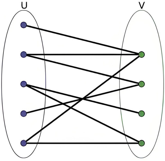
Figure 1.
Bipartite graph matching problem.
The mathematical properties of bipartite graph matching provide a natural modeling framework for task allocation problems: the binary topological compatibility allows the agent set U and target set V to form a natural bipartite structure, with edge weights representing interception effectiveness metrics. Additionally, adjacency matrix operations are well suited for GPU acceleration, ensuring that the time complexity meets real-time requirements.
2.2. Sequence-to-Sequence Model
A sequence-to-sequence model is a deep learning framework primarily designed for converting one sequence into another [20,21], commonly used in machine translation, text summarization, and speech recognition. It generally consists of an encoder and a decoder.
The encoder converts the input sequence into a fixed-length vector representation. Common encoder structures include recurrent neural networks (RNNs), long short-term memory (LSTM) networks, and gated recurrent units (GRUs). Taking RNNs as an example, when processing the input sequence, the input at each time step and the hidden state from the previous time step jointly determine the hidden state at the current time step. The hidden state at the final time step is typically regarded as the encoded representation of the entire input sequence. For instance, in machine translation, the encoder converts a source language sentence into a vector that encapsulates the semantic information of the source sentence.
The decoder generates the output sequence based on the context vector produced by the encoder. While generating the output sequence, the decoder typically combines the context vector with the previously generated portion of the output sequence to predict the next output element. Structures such as RNNs, LSTM, or GRUs can also be employed for the decoder. At each time step in generating the output sequence, the decoder calculates a probability distribution based on the current input (which may be the last generated word or character and the context vector) and then selects the next output element according to this distribution.
Sequence-to-sequence (Seq2Seq) models offer superior adaptability in task allocation scenarios with dynamically changing scales. Compared to traditional optimization algorithms, their ability to handle variable-length sequences overcomes the limitations of fixed-dimensional inputs. Furthermore, the encoder–decoder architecture enables strong online decision-making capabilities, supporting millisecond-level real-time responses.
2.3. Reinforcement Learning
Reinforcement learning is a machine learning technique that trains agents based on a trial-and-error process and a reward mechanism. This type of algorithm models the problem as a Markov decision process (MDP), where each decision depends solely on the current environmental state information, without considering prior state–action sequences. An MDP can be represented as a four-tuple . Here, S denotes the current environmental state information, A represents the agent’s action decision information, indicates the state transition probability of executing an action in the current state, and signifies the reward function. The objective of reinforcement learning algorithms is to find a policy, i.e., a rule for selecting actions in each state, such that the expected cumulative reward obtained by the agent following this policy from the initial state is maximized.
2.4. MADDPG Algorithm
The multi-agent deep deterministic policy gradient (MADDPG) algorithm is designed for multi-agent reinforcement learning [22]. It extends the traditional deep deterministic policy gradient (DDPG) algorithm to handle interactions and cooperation among multiple agents.
MADDPG employs the deterministic policy gradient theorem to calculate the policy gradients [23]. Similarly to the conventional DDPG algorithm, the policy gradient is calculated by taking the derivative of the value function with respect to the policy parameters. However, in a multi-agent environment, since the value function depends on the actions of multiple agents, it is necessary to account for the influence of other agents’ actions.
Each agent maintains its policy network for action generation and a value network for state value assessment. The policy network takes the agent’s observation as input and outputs a deterministic action, while the value network takes the observations and actions of all agents as input and outputs an estimated state value.
Compared to traditional reinforcement learning methods, MADDPG’s deterministic policy output is better suited for the continuous action space of route planning. Its global critic network implicitly coordinates agent behaviors, enabling more effective multi-target cooperation.
3. Interception Problem Model Construction
This study considers a scenario in which multiple agents cooperate to intercept multiple targets in a two-dimensional space, as shown in Figure 2. In the figure, the red solid circle represents the protected target P, the blue boat shape indicates the intelligent agent U, and the red boat shape represents the threat target V. Assume that the environment consists of multiple agents and multiple threat targets , where M represents the number of agents and represents the total number of threat targets in the environment. The following assumptions are made.
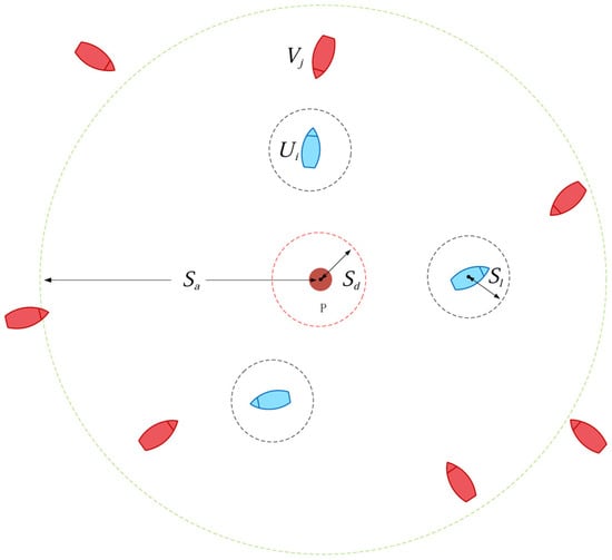
Figure 2.
Schematic diagram of the maneuver interception problem.
- (1)
- A static protected target P is located at the center of the scene, surrounded by several homogeneous agents U. At a distance, there are randomly scaled threat targets V. The two sides have opposing mission objectives: the agents maneuver forward to intercept the threat targets, while the threat targets continuously invade and approach the protected target.
- (2)
- The protected target has certain reconnaissance and detection capabilities, but it can only acquire the position and velocity information of threat targets within a radius of . Therefore, from its perspective, the number of threat targets is dynamically changing.
- (3)
- All threat targets are initially located outside the detection range and maneuver toward the protected target as their destination. Their control strategies are unknown, and they possess certain evasion capabilities. If they approach within a distance of , their intrusion mission is considered successful.
- (4)
- A certain long-distance communication link exists between the protected target and the surrounding agents, allowing the protected target to obtain agent position and velocity information and issue specific task assignments to maneuver the agents for interception. When an agent approaches a threat target within a distance of , the interception is considered successful.
- (5)
- To mitigate the potential threat posed by incoming targets and enhance the defense depth of the multi-agent system, it is necessary to rationally control the deployment of each agent to intercept threat targets. While ensuring the completion of all interception tasks, the targets should be intercepted at the farthest possible distance.
Therefore, the optimization objective of this problem is to determine the optimal task allocation relationship and multi-agent navigation control commands under the constraint of a limited number of deployed agents so that the multi-agent system intercepts the dynamically varying scale of threat targets at the maximum distance. This problem is a complex combinatorial optimization problem, including the two subproblems of task allocation (TA) and path planning (PP), which are described in detail below.
3.1. Threat Target Maneuver Model
Assume that, at the initial moment, the threat target is located outside the detection range of the protected target, with position coordinates , randomly oriented toward the protected target P at a speed of to invade. Considering that the threat target possesses a certain capacity for intelligent evasion, it will take evasive maneuvers upon detecting the presence of nearby intercepting agents. Here, the artificial potential field method from route planning is adopted as the evasion strategy, meaning that each agent exerts a repulsive force on the threat target, where the repulsive force increases as the distance between the threat target and the agent decreases. Thus, the velocity vector of the threat target is given by
where is the velocity vector directed toward the protected target, represents the position of the threat target, represents the position of agent i, is the distance between the threat target and agent i, and is the detection range of the threat target.
3.2. Task Assignment Model
Since the detection range of the protected target is limited, at time t, only N threat targets can be detected, , , and N increases over time. The task assignment model is constructed for M agents and N targets.
- (1)
- Model variables
For this task assignment problem, the optimization variable is the task assignment relationship between the agents and the targets. Here, an assignment matrix is introduced:
where represents whether the agent i is assigned to intercept the incoming target j. If assigned, ; otherwise, .
- (2)
- Optimization objective
The task assignment strategy must consider both the global interception probability and the defensive depth of the multi-agent system.
The interception success probability depends on the relative positions and velocities of the agents and threat targets, as well as the interception capabilities of the agents. Given the uncertainty in the maneuver strategy of the threat targets, the Euclidean distance between them is the most significant influencing factor. Since the interception success probability increases as the distance decreases, and, when the distance is less than a certain threshold, the interception is considered stable, the success probability of agent i intercepting threat target j and the global interception success probability are defined as
where represents the Euclidean distance between agent i and threat target j, denotes the interception range of the agent, is the interception probability decay coefficient , and is the task assignment matrix element.
The defensive depth of interception is expressed as the Euclidean distance between the threat target assigned to an interception task and the protected target:
where represents the Euclidean distance between threat target j and the protected target, is the matrix element of task allocation, and M is the number of agents.
Thus, the objective in optimizing task assignment is to maximize the task advantage function , as shown in the following equation:
where and are the weight adjustment factors for the interception success probability and the defensive depth, respectively; represents the global interception success probability; and is the Euclidean distance between the threat target and the protected target that is assigned the interception task.
- (3)
- Optimization constraints
In this problem, due to the uncertainty of the scale of incoming targets detected, in order to conserve defense resources and maximize the overall interception effect, a one-to-one task assignment strategy is adopted—that is, each agent is allocated only one target at each moment, as in the following equation:
In addition, to cope with changes in the situation of incoming targets in the environment, the multi-agent system uses an iterative assignment strategy constraint. That is, when new threat targets are added to the environment or when there is a significant change in the situation of current threat targets, it re-evaluates the current task assignment matrix and selects the optimal assignment strategy.
3.3. Route Planning Model
In the matching of agents and threat targets given in the task assignment phase, the purpose of route planning is for all agents to obtain the optimal continuous maneuver control commands to intercept the task targets as quickly as possible.
If a centralized route planning approach is used, where a central controller computes and assigns routes for all agents, an optimal solution theoretically exists. However, this approach is prone to route planning conflicts. Moreover, as the number of agents increases, the strategy space for decision-making grows exponentially, leading to higher computational resource demands for route planning. Given that maneuver control commands have high requirements for real-time performance and precision, long-range communication links may not reliably ensure the security and correctness of these commands. Therefore, a distributed maneuver control method is adopted here, where the task matching relationship is distributed to each agent, and the problem is solved from the perspective of a single agent. Based on the task assignment matrix derived from the task assignment phase, if , then agent i is assigned the real-time navigation control commands to intercept threat target j.
- (1)
- Model variables
In this environment, assume that the motion of agent i is controlled by two-dimensional continuous actions, where, at each time step, the control variables provided are and , where represents the velocity magnitude of the agent; is the current course.
Assuming that the position of agent i at time t is , then, at time , the position is updated as follows:
- (2)
- Optimization objective
To ensure that agents complete their interception tasks as quickly as possible, the minimization of the maneuver time for agent i to intercept target j can be chosen as the optimization objective. Let denote the time required for agent i to complete the interception of target j; then, the optimization objective is
Here, represents the optimal solution of the upper-level task allocation matrix.
- (3)
- Optimization constraints
This route planning problem mainly involves maneuverability constraints and interception task constraints.
The maneuverability constraint considers that an agent has a centripetal force limit when performing turning maneuvers. That is, when the velocity magnitude exceeds a certain threshold , the maximum allowable change in a single-step course is limited. This can be simplified using Equation (11):
where is the maximum lateral force provided to the agent, m is the mass of the agent, and represents the scalar speed of agent i.
The interception task constraint refers to the requirement that the Euclidean distance between the final destination of the agent’s route planning and the assigned target’s location must be less than its interception capacity range , i.e.,
4. Hierarchical MDP Model Construction
To address the strong coupling between task allocation and path planning in dynamic interception scenarios, this paper proposes an innovative hierarchical reinforcement learning (HRL) framework based on dynamic game equilibrium. Compared to traditional hierarchical frameworks [24,25,26] (e.g., HRL, MAXQ), the proposed model achieves efficient decision-making in dynamic environments through a multi-level optimization mechanism with spatiotemporal decoupling. The key innovations are as follows.
- (1)
- Hierarchical decision architecture design
As shown in Figure 3, the framework comprises two cooperative decision-making networks: a high-level task allocation network and a low-level path planning network. The high-level dynamic game-based allocator extends traditional static bipartite graph matching into a time-varying hypergraph matching problem , where the node set dynamically expands as new threat targets emerge, and the edge weights are updated in real time based on the target maneuvers. This network overcomes the fixed-node limitations of traditional optimization algorithms. The low-level distributed controller employs a curriculum learning-driven PER-MADDPG algorithm. By leveraging prioritized experience replay, it achieves diverse exploration in early training stages and focuses on critical states in later stages.
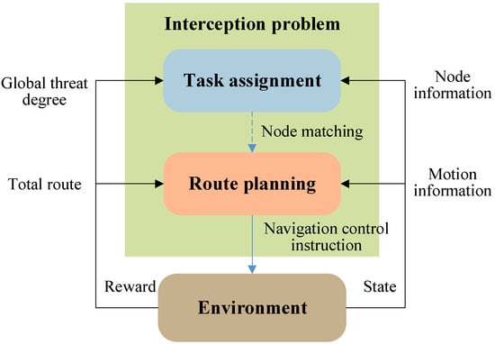
Figure 3.
Hierarchical reinforcement learning framework.
- (2)
- Innovative mechanism design
This model breaks through the limitations of conventional hierarchical frameworks through the following multi-level decoupling mechanisms.
- (i)
- Spatiotemporal decoupled hybrid triggered update mechanism
In contrast to traditional hierarchical models that rely on goal-driven updates (e.g., lower-level policies in HAC depend on high-level sub-goal states [27,28]) or time-scale-based updates (e.g., FeUdal networks where high and low levels operate on different time resolutions [29,30]), this model adopts a hybrid triggering mechanism based on spatiotemporal decoupling. Specifically, the high and low levels normally update asynchronously at dual time scales—path planning and interception environments are updated at every step, while task allocation is updated every T steps. Additionally, any change in the target node set triggers a forced update of the high-level task allocation. This hybrid mechanism suits the long-duration nature of interception tasks, avoiding the sparsity of purely event-triggered schemes while still responding promptly at critical moments.
- (ii)
- Hybrid decision topology
At the high level, a global attention matching network [31,32] is used to extract cooperative features across agents and generate task allocation policy networks , overcoming the local perception limitations of traditional graph neural networks (GNNs). At the low level, a federated reinforcement learning architecture is constructed, where each agent maintains its own local path planning policy network .
- (iii)
- Bidirectional reward coupling architecture
The high-level network optimizes task allocation from a strategic perspective using task rewards based on the interception success probability and defensive depth. The low-level network conducts path planning from a tactical perspective using rewards based on the relative positions between agents and targets. Together, these networks achieve a differentiable game equilibrium, addressing the limitations of isolated reward function design in traditional HRL frameworks.
As shown in Table 1, the hierarchical MDP model significantly improves the decision-making efficiency through the decomposition of tasks across multiple time scales. Specifically, the upper-level strategy (slow time scale) and the lower-level strategy (fast time scale) have systematic differences in the design of the state space, action space, and reward function. This hierarchical architecture is one of the core innovations of this study.

Table 1.
The differences between the high and low levels of the MDP model.
4.1. High-Level MDP Model
The task assignment model is converted into an MDP model based on maximum weight matching in a bipartite graph. In this bipartite graph , the set of agents forms nodes on one side of the graph, with M being the number of agents, and the set of detected threat targets forms nodes on the other side, with N being the number of detected threat targets (N changes over time). When agent i is assigned to intercept threat target j, an edge is added between nodes and , with the edge weight defined based on the expected benefits from the interception of threat targets by agents (interception probability and defensive depth). The objective of the maximum weight matching for this bipartite graph is to find a matching that leads to
where no two edges in M share the same endpoint. Traditional methods can obtain optimal solutions in polynomial time, but, in dynamic or online decision-making scenarios (e.g., real-time task assignment, dynamic network flow scheduling), challenges arise in terms of computational time and adaptability.
The high-level MDP model is represented by the tuple , where is the state space of the maximum weight matching problem in the bipartite graph, i.e., the information of the bipartite graph nodes extracted from the interception problem environment; is the action space of the matching problem, i.e., the node matching relationships in the bipartite graph; is the reward function of the matching problem; and is the state transfer probability of the matching problem. The objective of the high-level MDP model is to find an optimal high-level strategy —that is, the probability of mapping to —so as to maximize the cumulative discounted reward at the high level.
where is the discount factor of the higher level, with .
The following sections describe the state space , action space , and reward function in detail in the high-level MDP tuple.
- (1)
- State space
At time t, the state consists of the node and edge information in the bipartite graph matching problem. This mainly comprises agent node set , target node set , edge set , matched node sets and , matched edge set , and available edge set .
- (2)
- Action space
At time step t, the action involves each agent selecting an edge from the available edge set for matching. If both endpoints of the edge are unmatched, the matching is successful; otherwise, it is invalid. Once executed, the action marks related nodes as matched and removes them from subsequent decisions. The node matching relationships of each edge represent the task allocation between agents and targets.
- (3)
- Reward function
When an agent selects an edge , it receives a normalized edge weight reward :
where represents the value weight of the selected edge based on the interception success probability and defensive depth, calculated using the task advantage function from Section 2.2, and is the maximum possible total matching weight in the bipartite graph or the estimated upper bound, normalizing the reward to enhance the training stability. No reward is given for unmatched edges or invalid actions.
4.2. Low-Level MDP Model
The low-level MDP model is represented as a tuple , where is the state space for the route planning problem, containing the position and velocity information of agent i and its assigned target; is the action space for the route planning problem—specifically, the course and speed for agent i; is the reward function for the route planning problem; and is the state transition model for the route planning problem. The objective of the low-level MDP model is to find the optimal low-level strategy for each agent i—that is, the mapping probability from to —so as to maximize the low-level cumulative discounted reward .
where is the discount factor of the low level, .
The following sections describe the observation space , action space , and reward function in detail in the low-level MDP tuple.
- (1)
- State space
When solving the low-level route planning problem, the state for low-level agent i includes its own location information and motion information , as well as the assigned task target location information , motion information , and interception state information obtained through the data link.
- (2)
- Action space
The low-level agent action is the maneuver control command for each agent—that is, the course adjustment value and the speed .
- (3)
- Reward function
Based on the optimization objectives and constraints from Section 2.2, the following reward function is designed to evaluate the agent state. When agent i is assigned to intercept a target, to guide it to complete the task as quickly as possible, it receives a negative reward at each time step t; when the agent approaches the target to the effective range and completes an interception task, it receives a positive reward for task completion; when the incoming target evades the interception and approaches the protected target to a dangerous distance , it receives a large negative reward .
To guide the agent to quickly occupy an advantageous position and improve the interception efficiency, an analysis of the distance and angle benefits is conducted for , i.e., , where and are the corresponding weight factors.
- (i)
- Distance reward
- (ii)
- Angle reward
To guide the agent to intercept with a certain lead angle, occupy an advantageous interception position between the incoming threat and the protected target, and avoid the phenomenon of tailing the target, the relative bearing angles and of the agent and the incoming threat with respect to the protected target can be calculated based on their position information. The smaller the relative bearing angle , the higher the interception efficiency, as it ensures that the agent is positioned between the incoming threat and the protected target, improving the likelihood of successful interception. Here, a negative exponential function is used, and an angular adjustment coefficient is introduced.
5. Hierarchical Reinforcement Learning Algorithm Process
For the hierarchical MDP model of the interception problem described above, a hierarchical reinforcement learning algorithm based on curriculum learning is applied. This algorithm involves two main modules: a high-level task assignment module and a low-level route planning module. The high-level module uses a sequence-to-sequence policy gradient reinforcement learning algorithm to solve the bipartite graph matching problem, while the low-level module employs a prioritized experience replay-based MADDPG algorithm to solve the distributed route planning problem. The detailed structure is shown in Figure 4.
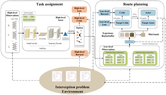
Figure 4.
Hierarchical reinforcement learning algorithm architecture.
The task assignment module’s policy network mainly includes structures such as a graph encoder, a sequence decoder, and an attention module. First, the high-level state space extracts agent and target position information from the environment, converting this into bipartite graph feature information, including nodes, edges, and dynamic weights, and passes it to the high-level actor network. The high-level actor network employs a sequence-to-sequence model (Seq2Seq) to obtain bipartite graph matching decisions, consisting of two key parts: a graph encoder and a sequence decoder. The graph encoder utilizes graph embedding to convert bipartite graph node feature information into low-dimensional vector representations and then passes the graph embeddings to the sequence decoder. The sequence decoder computes the probability distribution of node matching based on node embeddings, edge indices, and available actions. After the high-level actor network sampling outputs the specific matching results to the low-level route planning module, it interacts with the environment to generate rewards and new observations, and the high-level critic network updates the value estimates, updating the high-level actor–critic network parameters with the goal of minimizing the high-level loss.
The route planning module consists of a low-level actor–critic network, a target network, Ornstein–Uhlenbeck noise, and a buffer. First, the low-level observation space receives agent-to-target task matching from the high level and extracts the motion state of the assigned target from the environment, feeding this data into the low-level actor network. Ornstein–Uhlenbeck noise is introduced to enhance exploration, generating an initial route planning state–action sequence . The low-level critic network calculates the value estimates of actions based on the current observation state and the actor network’s output and uses policy gradient updates to guide the optimization of the low-level actor network. The target network is updated periodically to provide relatively stable target values for the low-level actor–critic network, ensuring that the network gradually optimizes and converges so that the agents can successfully find the optimal path to their targets in complex and dynamic environments. The buffer stores state–action sequences generated during interactions with the environment, improving data utilization for effective network parameter updates.
The overall process of the algorithm is summarized as follows.
- (1)
- Initialization of the interception problem environment
Initialize the grid size of the environment and the numbers of agents and threat targets and generate their initial positions, courses, and speeds.
- (2)
- Task assignment based on bipartite graph matching
Convert environmental information into a bipartite graph (U, V, E), initialize nodes for assignment, and collect available edge information. A sequence-to-sequence reinforcement learning strategy (GNN encoder + decoder) is used to evaluate the available edges, sample and execute matching actions, calculate normalized rewards, remove conflicting edges, and iterate until no available edges remain or conditions are met.
- (3)
- Multi-agent route planning
At each time step, each agent’s actor network executes maneuver control actions, the environment updates the agents’ states and target states (task assignment and interception determination), and the critic network evaluates states and actions and updates the parameters for all agents, with soft updates of the target networks entering the next time step.
- (4)
- Training and testing
Simulate multiple rounds, record and analyze interception success rates and cumulative rewards, adjust hyperparameters, and compare with baselines to evaluate algorithm performance.
During the training phase, a curriculum learning method is used for gradual training. In simpler training courses, the high-level task assignment module is trained assuming that threat targets employ straightforward control strategies (moving directly toward the protected target). In this phase, the task assignment network is trained to maximize the interception effectiveness while ignoring the subsequent maneuver control of agents. In the more complex training phase, the trained task assignment network is applied to the real interception environment, and the route planning module’s AC neural network is trained to develop a distributed maneuver control decision-making network.
The testing phase is relatively straightforward. The high-level task assignment module determines task target matching based on the relative positions of detected threat targets and agents in the interception problem environment and then outputs these assignments to the low-level route planning module for real-time route planning. The agents compute their respective control commands and feed them back to the interception problem environment for environmental updates.
The following sections provide a detailed explanation of the specific processes of the high-level and low-level algorithms.
5.1. Sequence-to-Sequence Model-Based Policy Gradient Reinforcement Learning Algorithm
This algorithm integrates the advantages of the sequence-to-sequence model and policy gradient reinforcement learning, utilizing graph neural networks to continually interact with the bipartite graph matching task, thereby learning the optimal task assignment strategy. In each training round, the algorithm encodes the bipartite graph through a graph neural module, using a decoder to generate action distributions, selecting actions, obtaining rewards, and finally updating the network parameters through the actor–critic mechanism to progressively improve the task assignment efficiency and accuracy. The following is a detailed explanation of the algorithm’s network design and training process.
- (1)
- Policy network design based on the sequence-to-sequence model
To learn a probability strategy for edge selection, we adopt a policy gradient-based update framework, where represents the policy network parameter. When a matching trajectory is sampled, i.e., , its return is recorded as [33,34,35]:
We expect the policy-based method to learn an optimal strategy that maximizes the expected value of the return :
Skipping the derivation process, the update rule for the policy gradient algorithm is as follows [36]:
By increasing the probability of selecting high-return actions, the optimal strategy is achieved. Additionally, a baseline can be introduced to reduce variance, usually estimated as the state value function , helping the algorithm to better understand the potential value of each state and distinguish which actions lead to better or worse outcomes than expected.
Given the sequential nature of bipartite graph matching, where each step’s selected edge not only affects the current reward but also changes the set of available edges, the comprehensive perception of the global structure and local relations is necessary. The matching process can be analogized to generating a sequence (a sequence of edges), and a Seq2Seq encoding–decoding framework-based policy network is used for solution. The policy network consists of a graph encoder and a decoder, incorporating an attention mechanism to enhance the decision precision.
Encoder stage: The graph encoder encodes features of each node in the graph, generating latent vector representations, or integrates global contextual information (e.g., matched edge set) into a hidden vector based on environmental needs.
Decoder stage: It generates a score for each edge in the available edge set and obtains a probability distribution via Softmax, allowing for action sampling or greedy selection.
Attention mechanism: During decoding, different attention weights can be assigned to different nodes/edges to focus on potentially important candidate edges, enhancing the selection efficiency.
Compared to typical feedforward networks (MLP), the Seq2Seq model with an attention mechanism is better at capturing sequence or structure dependencies from variable-length, dynamic inputs, making it particularly well suited for structured problems like bipartite graph matching.
- (2)
- Training process
To improve the sample utilization efficiency, we employ an actor–critic network mechanism for updates. Let θ represent the learnable parameter of the actor network (Seq2Seq + Attention), and L is the maximum length of each training episode. The core process is described in Algorithm 1.
| Algorithm 1 Policy gradient-based bipartite graph matching sequence decision-making |
| 1: Initialize: Policy network (encoder and decoder) Function (GenerateBipartiteGraph) Hyperparameters (discount factor, learning rate, etc.) |
| 2: for episode = 1, 2, …, do |
| 3: Generate a bipartite graph either randomly or based on the interception task environment and initialize the bipartite graph environment (matching set, available edge set, etc.) |
| 4: Obtain initial state based on |
| 5: , , |
| 6: while not done do |
| 7: Obtain node features x, available edge indices , etc., from state |
| 8: Get the probability distribution of available edges from policy network |
| 9: Sample actions based on this distribution |
| 10: |
| 11: Record into , Record into |
| 12: |
| 13: end while |
| 14: , |
| 15: for t = T − 1 down to 0 do |
| 16: |
| 17: |
| 18: end for |
| 19: |
| 20: for t = 0 to T − 1 do |
| 21: |
| 22: end for |
| 23: |
| 24: end for |
5.2. Route Planning Based on MADDPG
To address the multi-agent route planning problem under a complex maneuvering model, this study employs the multi-agent deep deterministic policy gradient (MADDPG) algorithm with prioritized experience replay (PER) to improve the training efficiency and performance in multi-agent reinforcement learning. In this algorithm (Algorithm 2), each agent has its own actor and critic networks. Through network initialization, interaction with the environment, experience data storage, PER-based training, and network parameter updates, multiple agents can learn effective policies to accomplish their tasks. The PER technique prioritizes experience sampling and updates based on importance, ensuring that more valuable experiences have a greater impact on learning, thereby accelerating the training process and improving the learning outcomes.
- (1)
- PER-based MADDPG algorithm architecture
Actor network: Each agent has an independent actor network , which takes the observed states of agent i as input and outputs the deterministic action . The purpose of this network is to learn an optimal action selection policy that maximizes the cumulative reward. During training, the actor network parameter is updated using the policy gradient method, guided by the evaluation from the critic network:
where represents the actor network, and is the sample drawn from the experience replay buffer.
Critic network: Each agent’s critic network takes the states and actions of all agents as input, i.e., , and outputs a scalar value representing the Q-value (expected cumulative reward) under the given state and action. This network evaluates the quality of the current policy and provides gradient update information for the actor network. The critic network updates its parameter by minimizing the error between the predicted Q-value and the target Q-value. The target Q-value is typically computed using the Bellman equation:
where is the discount factor.
Target networks: To stabilize the training process, each agent maintains corresponding target actor and target critic networks. The target networks are updated using a soft update strategy, where the parameters of the target network slowly converge to those of the main network, reducing the high variance and instability in training.
Ornstein–Uhlenbeck (OU) noise: To enhance exploration, OU noise is added to the actions chosen by the actor network. OU noise exhibits a temporal correlation, making it particularly suitable for control tasks with physical inertia properties. As training progresses, the noise amplitude gradually decreases, ensuring a smooth transition from exploration to exploitation.
Prioritized experience replay (PER): During agent–environment interaction, experience data is stored in the replay buffer . In training, a batch of samples is randomly drawn from the buffer instead of directly using newly generated experience, thereby breaking the correlations between samples and improving the training stability and efficiency. To further enhance the training efficiency, a PER mechanism is introduced to assign a priority to each experience based on its significance (typically measured by the TD error). Samples are drawn based on their priority rather than randomly, ensuring that more impactful experiences are used more frequently in training. To counteract potential biases from prioritized sampling, importance sampling weights are calculated via and are used when updating the critic network.
- (2)
- Training process
The actor and critic networks are built using fully connected layers with ReLU activation functions. The OU noise is dynamically scaled based on the action space range, ensuring exploration within an effective control region. The training process runs for a fixed number of episodes (e.g., 10,000), during which agents continuously refine their strategies and optimize their decisions based on the reward signals. After training, the strategy’s effectiveness is assessed through multiple rounds of testing in a route planning environment using the reward function.
| Algorithm 2 PER-based MADDPG algorithm process |
| 1: Initialize: Actor network and critic network for each agent i. |
| Target networks and , and , |
| Experience replay buffer with a capacity of M and priority parameter |
| PER parameters: (priority exponent), (importance sampling exponent). |
| 2: for episode = 1, 2, …, do |
| 3: Reset the environment and obtain the initial state. |
| 4: for t = 0, 1, …, do |
| 5: for each agent i do |
| 6: Select action based on the current policy (where is OU noise). |
| 7: end for |
| 8: Execute the joint action , and obtain rewards and the next state from the environment. |
| 9: Store in , and let priority be |
| 10: for each agent i do |
| 11: Sample from based on priority |
| 12: Compute importance sampling weight |
| 13: Compute the target Q-value: |
| 14: Update critic network by minimizing the weighted MSE loss |
| 15: Update actor network using policy gradient |
| 16: Update priority based on TD error. |
| 17: end for |
| 18: Soft update target networks: , |
| 19: |
| 20: end for |
| 21: end for |
6. Experiment
For this work, we established a simulated interception environment and trained the policy networks using the proposed hierarchical reinforcement learning algorithm. We then analyzed the effectiveness of this method and compared the performance metrics with those of other algorithms, finally validating the impact of curriculum learning on network training.
6.1. Experimental Environment and Parameter Configuration
The experiments were conducted on a platform equipped with an Intel Core i9-10980XE CPU, an NVIDIA RTX 2080Ti GPU, and 128 GB of RAM. For the software, PyTorch 2.0 was used as the deep learning training framework, and OpenAI Gym served as the reinforcement learning environment framework.
During training, curriculum learning was adopted to conduct phased training for the interception task. Initially, bipartite graph nodes were randomly generated, and the task assignment module was trained on simple tasks. Subsequently, the trained model was applied to the route planning module for global interception task training to tackle more complex problems. After numerous experiments and hyperparameter tuning, the primary parameters of the simulation environment were established, as shown in Table 2.
Table 2.
Experimental parameters.
The parameter selection strictly followed the following dual criteria.
- (1)
- Physical realism constraint: All environmental parameters (including the grid resolution, agent movement speed, and interception distance threshold, etc.) were dimensionless and processed based on the actual physical system to ensure that the simulation environment maintained geometric similarity to the real scene.
- (2)
- Training robustness optimization: For the key hyperparameters in the hierarchical algorithm architecture (such as the dual-time-scale learning rate, hierarchical discount factor, etc.), a grid search strategy guided by Bayesian optimization was adopted to systematically tune the parameters in the standard validation scenario, finally selecting the parameter combination that minimized the cumulative reward variance.
6.2. Method Effectiveness
6.2.1. Performance Analysis of Different Numbers of Agents
In order to demonstrate the generality and effectiveness of the algorithm in completing multi-agent interception tasks, this section considers the interception task for targets of varying scales with different numbers of agents. Given the training performance limitations of the experimental platform, the number of agents is set to 5, 10, and 15, respectively (with the number of incoming targets randomly set to twice the number of agents).
To ensure the validity of the results, different random seeds are adopted to perform training 10 times in each scenario, with each training step involving 300,000 iterations. The average reward obtained by each agent in the multi-agent system for completing the interception task is used as a reference performance indicator for the algorithm. As shown in Figure 5, the average reward increases rapidly within the first 20,000 iterations for each scenario, and it gradually stabilizes and converges around the 50,000th iteration, indicating that the agents have learned the optimal interception strategy. At the end of the training, the average interception reward for each agent decreases as the problem scale increases. This is due to the fact that, as the number of agents and threat targets increases, the interception task becomes more complex. Consequently, the increased interception time during the route planning phase leads to higher negative rewards for time steps, resulting in a decrease in the total interception reward.

Figure 5.
Reward curves of the algorithm in scenarios with different numbers of agents.
The simulation diagrams in Figure 5, Figure 6 and Figure 7 present the interception process of the multi-agent system in scenarios with different scales. In the figures, the blue inverted triangles stand for threat targets, the boat icons stand for agents, and the central black star is marked as the protected target. When threat targets enter the detection range of the red circle, the multi-agent system executes an interception strategy. The red arrows indicate the task matching relationships. When an agent maneuvers to a position where the distance to the threat target is less than its operating range, it can perform the interception action. Subsequently, the threat target loses its maneuverability (turned into a red cross). The task ends when all threat targets in the environment are intercepted.
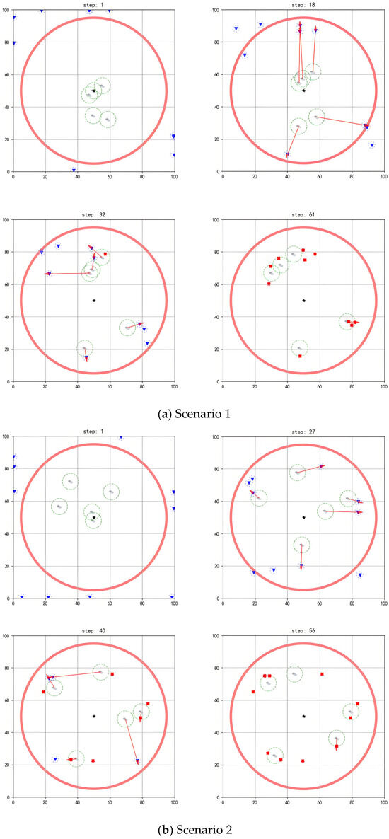
Figure 6.
Performing interception task with 5 agents.
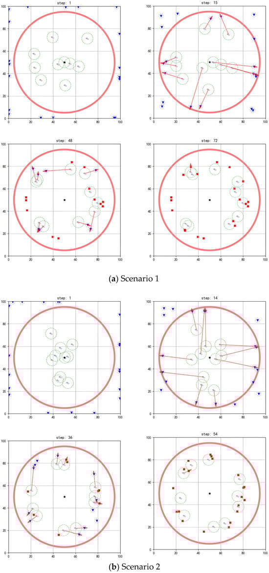
Figure 7.
Performing interception task with 10 agents.
As shown in Figure 6a, initially, the agents are randomly deployed around the protected target, with threat targets outside the detection range preparing to invade (step = 1). Once a threat target enters the detection range, task assignment and interception route planning are performed based on the positional advantages of each agent (step = 18). When the agents approach threat targets within their operating ranges, they complete the current interception task and are then assigned subsequent target tasks (step = 32). Through multiple task reassignments and real-time route planning, the multi-agent system completes the interception of all threat targets (step = 61).
As shown in Figure 6b, when the threat target approaches the agents within a certain distance and detects their interception behavior, it will take evasive actions. For example, the two threat targets in the upper-left corner escape upwards (step = 27). However, the agents can move toward the predicted location of the threat targets based on their evasion directions for interception (step = 40), finally completing all interception tasks (step = 56).
Figure 7 and Figure 8 show that, when different numbers of agents face a larger scale of threat targets, the existing algorithm still achieves good interception results.
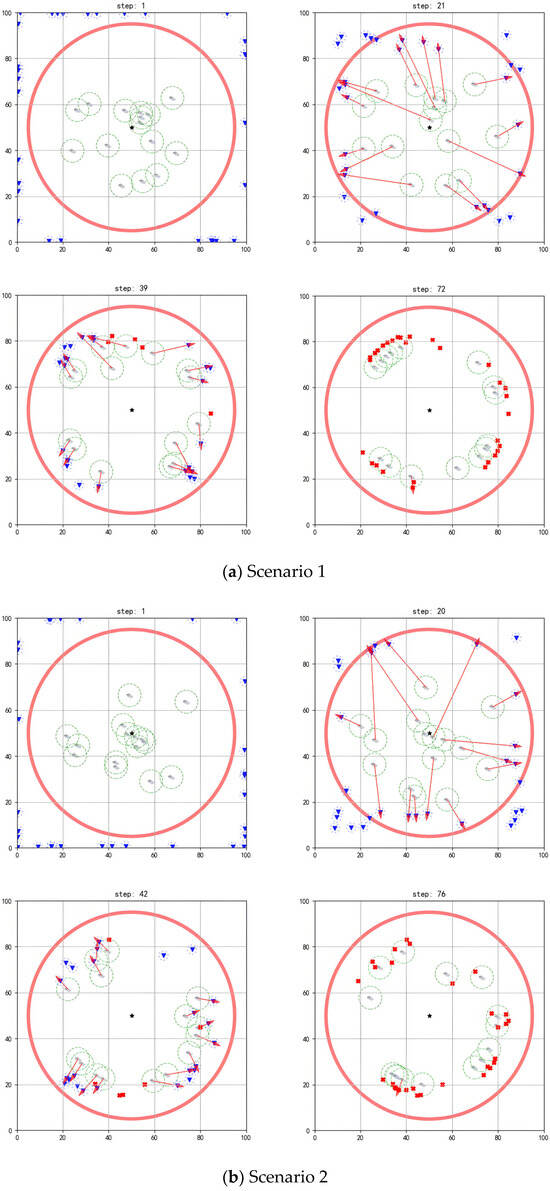
Figure 8.
Performing interception task with 15 agents.
6.2.2. Ablation Experiment
To study the impact of components such as the curriculum learning strategy, Seq2Seq structure, attention mechanism, and PER mechanism on the overall performance of the hierarchical reinforcement learning algorithm, an ablation experiment is designed. Based on the initially designed network structure, this experiment compares the contributions of each mechanism to the algorithm’s performance by removing certain strategies or disabling specific structures and calculating the average reward after stable training. The experimental scenario involves 15 agents intercepting 30 incoming targets, with the results shown in Table 3. The conclusion drawn is that the Seq2Seq structure contributes the most to the algorithm; removing this module results in an average reward drop to 8.28, corresponding to an ablation loss of 11.64%. The curriculum learning strategy ranks second, contributing 8.41%, while the attention mechanism and PER mechanism contribute 5.43% and 4.74%, respectively.
Table 3.
Contribution comparison in ablation experiment.
6.3. Algorithm Comparison
This work proposes a hierarchical framework for reinforcement learning-based interception algorithm (HFRL-IA) and optimizes its structure partially according to the characteristics of the maneuver interception problem. To demonstrate the superiority of the algorithm, comparative experiments are conducted between the reinforcement learning algorithm under the overall framework and traditional algorithms under the hierarchical framework. The reinforcement learning algorithm under the overall framework adopts the classic MADDPG algorithm as a baseline, with a similar policy network and value network to those used in this work, and all other parameters remain the same. The hierarchical framework for comparison employs the control variable method to replace the subtask modules in the algorithm. The task allocation module is replaced with the Hungarian algorithm to form the hierarchical framework Hungarian algorithm (HF-HA), or the route planning module is replaced with the genetic algorithm to form the hierarchical framework genetic algorithm (HF-GA).
The four methods mentioned above are used to perform training multiple times in the interception environment with different scales of agents (let the number of agents be 5, 10, and 15, respectively, and the number of incoming targets is randomly set to twice this value). Moreover, the algorithm’s performance is evaluated from two aspects: the average reward and the interception rate. The average reward is used to compare the learning effectiveness and strategy optimization capabilities of different algorithms. A higher reward or faster convergence indicates stronger optimization capabilities of the algorithm. The interception rate reflects the proportion of targets intercepted by the agents. A higher interception rate indicates better task completion performance.
Figure 9 shows the reward curves of different algorithms with 5, 10, and 15 agents. In the figures, it is shown that all methods can converge within the training steps. HFRL-IA optimizes the algorithm structure based on the characteristics of the interception problem, which enables more effective coordination among multi-agent cooperation. Therefore, its average reward at each step is the highest across all scenarios, and its hierarchical architecture allows for faster convergence. Compared to HFRL-IA, MADDPG has a slightly lower average reward because it does not optimize the target scale changes and maneuver characteristics in the environment, and its global network architecture results in slower convergence. As the scale of agents increases, the algorithm performance gap grows. HF-GA has an even lower average reward and slower convergence, as the genetic algorithm, being a heuristic search method, finds the optimal solution through many iterations when dealing with complex problems. However, in dynamic and maneuver interception environments, it struggles to quickly adapt to the environment and generate the optimal path, leading to reduced agent efficiency. HF-HA has a faster convergence speed compared to HF-GA, but its final average reward is the lowest. This is attributed to the fact that, while the Hungarian algorithm is efficient for static task allocation, it struggles to adjust its task assignment strategies in multi-agent dynamic coordination scenarios as the environment changes, resulting in poorer overall performance.
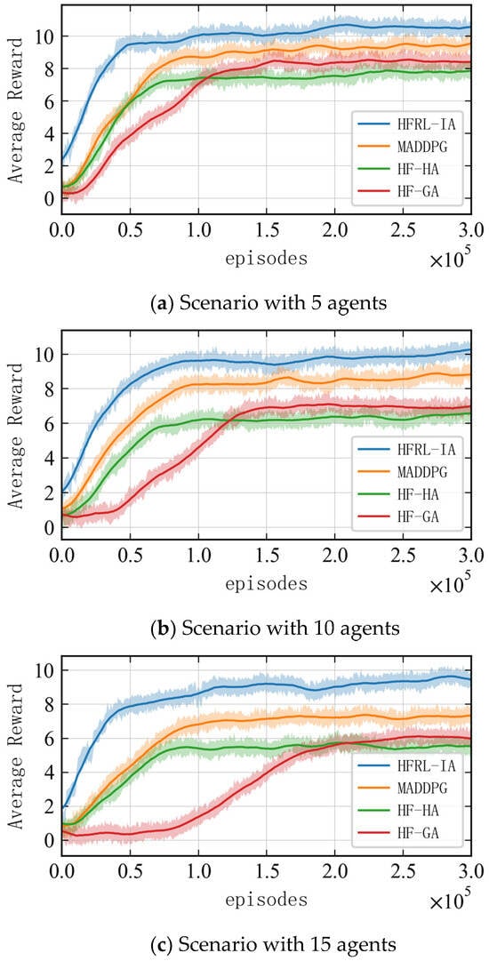
Figure 9.
Reward curves of different algorithms.
The experimental results show that the HFRL-IA algorithm exhibits superior reward convergence characteristics during the training process. Taking a typical 10-agent interception scenario as an example, the cumulative reward that it ultimately achieves is 22.51% higher than that of the traditional end-to-end MADDPG algorithm, and the convergence speed is increased by approximately 40% when achieving the same reward. This advantage mainly stems from the explicit modeling capability of the hierarchical framework for collaborative strategies.
To systematically evaluate the interception performance of each algorithm in different-sized intelligent agent clusters, this study conducted 100 independent repeated experiments for each algorithm configuration. Given that the interception experiment results exhibit typical binary classification characteristics (success/failure), and considering the statistical characteristics of small sample data, we employed the Wilson score interval estimation method for confidence level assessment. This method has better statistical robustness in cases of small samples and extreme proportions. The final results are presented in Table 4 (interception rate statistics table) and Figure 10 (interception rate trend line graph).
Table 4.
Statistics of interception rates for different algorithms.

Figure 10.
Interception rates of different algorithms.
Figure 10 further shows the changes in the interception success rate for the four algorithms under different agent scales through multiple simulation experiments. As seen in the figure, as the scale of agents and threat targets increases, the interception rate of all four algorithms decreases. This occurs because the increased complexity of the task raises the likelihood of the threat target breaching the defense, which aligns with the decreasing average interception reward seen in Figure 8 as the scale increases. Among all the algorithms, HFRL-IA consistently achieves the highest interception success rate, indicating that it performs the best in interception and utilizes the most reasonable strategies.
After a systematic analysis of the experimental data, it is clearly observable that the HFRL-IA algorithm demonstrates significant advantages in all performance indicators. Among all compared algorithms, this algorithm consistently maintains the leading position in the interception success rate. This phenomenon fully validates the superiority of its interception efficiency and the rationality of its strategy design. Especially in the representative 10-agent interception scenario test, compared with the traditional end-to-end MADDPG method, the HFRL-IA algorithm increased the interception success rate from the baseline level of 61.13% to 87.48%, achieving a remarkable improvement of 26.35 percentage points.
6.4. Method Limitations
Although the proposed algorithm demonstrates strong performance in large-scale interception scenarios, it still lacks effective strategies for situations where the number of incoming targets N’ significantly exceeds the number of agents M. To analyze this limitation, a progressive overload test was conducted using the overload factor . The number of agents M was set to 5, 10, and 15, respectively, and each configuration was tested in 100 interception scenarios with varying numbers of incoming targets. The relationship between the interception success rate and target scale is shown in Figure 11.
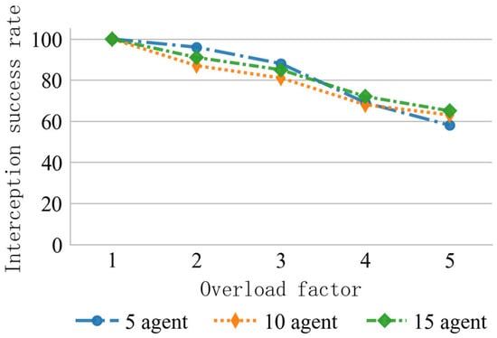
Figure 11.
Interception rate under different overload factors.
According to the data, when , the proposed method maintains a success rate above 80% across all agent configurations. However, when = 5, the success rate drops sharply to around 60%. Based on queuing theory stability analysis, when the multi-agent service queue reaches its task capacity limit, resource contention causes the task allocation strategy to fail, pushing the system into an unstable state. A typical failure scenario is illustrated in Figure 12.
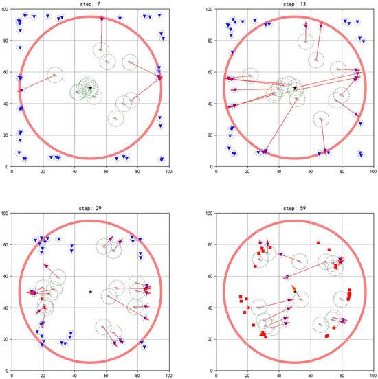
Figure 12.
Representative interception failure under high overload factor.
In this scenario, each agent initially allocates tasks and intercepts threats based on the optimal strategy (step = 7). However, when the overload factor becomes too large and the number of threats exceeds the system’s critical capacity, all agents complete their task allocation at the same time (step = 13). This leads to queue overflow, causing the task allocation mechanism to fail—i.e., newly emerging threats have no available agents to respond (step = 29). By the time that the agents have completed their current tasks and prepare for the next interception round, the threats have already breached the defense line (step = 59).
7. Conclusions
This paper proposes an innovative solution based on hierarchical reinforcement learning for the problem of multi-agent cooperative maneuver interception in dynamic environments. Through the design of a novel hierarchical decision-making architecture, the complex interception task is decoupled into two optimization stages: dynamic task allocation and distributed path planning. The upper-level dynamic task allocation is formulated as a bipartite graph matching problem, where a sequence-to-sequence reinforcement learning model is employed to achieve the incremental assignment of emerging threat targets—overcoming the limitations of traditional Hungarian algorithms in handling dynamically expanding target sets. In the lower-level path planning stage, the integration of prioritized experience replay (PER-MADDPG) and curriculum-based progressive training significantly improves the training stability. Simulation experiments conducted in interception scenarios demonstrate the effectiveness and advantages of the proposed algorithm.
However, the current framework still lacks sufficient adaptability in ultra-large-scale threat environments. Future work will explore (1) federated reinforcement learning architectures [37,38] to integrate distributed perception with centralized decision-making under high-overload conditions; (2) transfer learning mechanisms for rapid adaptation to unseen threat configurations based on meta-reinforcement learning principles [39,40]; (3) hardware-in-the-loop simulation platforms combining FPGA acceleration [41] with digital twins for real-time validation; and (4) the integration of heterogeneous multi-agent [42,43] dynamic collaboration strategies to further enhance the interception performance in complex scenarios.
In summary, this study presents a new methodological framework for multi-agent cooperative interception in dynamic adversarial environments, with significant application potential in areas such as aquaculture protection, maritime security, and ocean environmental monitoring.
Author Contributions
Conceptualization, Q.H., Y.L., Z.L., J.X., M.C. and J.L.; methodology, Q.H., Y.L., Z.L., J.X., M.C. and J.L.; software, Q.H., Y.L., Z.L., J.X., M.C. and J.L.; validation, Q.H., Y.L., Z.L., J.X., M.C. and J.L.; formal analysis, Q.H., Y.L., Z.L., J.X., M.C. and J.L.; investigation, Q.H., Y.L., Z.L., J.X., M.C. and J.L.; resources, Q.H., Y.L., Z.L., J.X., M.C. and J.L.; data curation, Q.H., Y.L., Z.L., J.X., M.C. and J.L.; writing—original draft preparation, Q.H. and Y.L.; writing—review and editing, Q.H. and Y.L.; visualization, Q.H. and Y.L.; supervision, Q.H., Y.L., Z.L., J.X., M.C. and J.L.; project administration, Q.H., Y.L., Z.L., J.X., M.C. and J.L.; funding acquisition, M.C. All authors have read and agreed to the published version of the manuscript.
Funding
This research was funded by the National Natural Science Foundation of China, grant number 52402370.
Data Availability Statement
The data is contained in the article.
Conflicts of Interest
The authors declare no conflicts of interest.
Abbreviations
The following abbreviations are used in this manuscript:
| MDP | Markov decision process |
| HFRL-IA | Hierarchical framework for reinforcement learning-based interception algorithm |
| PER-MADDPG | Prioritized experience replay multi-agent deep deterministic policy gradient |
| MAS | Multi-agent system |
| MADDPG | Multi-agent deep deterministic policy gradient |
| TD3 | Twin delayed deep deterministic policy gradient |
| ITATP-LC | Intelligent task allocation and trajectory planning with limited communication |
| MADRL | Multi-agent deep reinforcement learning |
| UAVs | Unmanned aerial vehicles |
| GPU | Graphics processing unit |
| RNN | Recurrent neural network |
| LSTM | Long short-term memory |
| GRU | Gated recurrent unit |
| Seq2Seq | Sequence-to-sequence |
| TA | Task allocation |
| PP | Path planning |
| HRL | Hierarchical reinforcement learning |
| MAXQ | Max-Q value function decomposition |
| GNNs | Graph neural networks |
| HF-HA | Hierarchical framework Hungarian algorithm |
| HF-GA | Hierarchical framework genetic algorithm |
References
- Qu, C.; He, J.; Li, J.; Fang, C.; Mo, Y. Moving target interception considering dynamic environment. In Proceedings of the 2022 American Control Conference (ACC), Atlanta, GA, USA, 8–10 June 2022; pp. 1194–1199. [Google Scholar]
- Sun, S.; Cai, D.; Zhang, H.T.; Xing, N. Reinforcement Learning-Based MAS Interception in Antagonistic Environments. IEEE/CAA J. Autom. Sin. 2024, 11, 270–272. [Google Scholar] [CrossRef]
- Sahoo, S.K.; Choudhury, B.B.; Dhal, P.R. Exploring the role of robotics in maritime technology: Innovations, challenges, and future prospects. Spectr. Mech. Eng. Oper. Res. 2024, 1, 159–176. [Google Scholar] [CrossRef]
- Sharma, A.; Shoval, S.; Sharma, A.; Pandey, J.K. Path planning for multiple targets interception by the swarm of UAVs based on swarm intelligence algorithms: A review. IETE Tech. Rev. 2022, 39, 675–697. [Google Scholar] [CrossRef]
- Sujit, P.B.; Sinha, A.; Ghose, D. Multiple UAV task allocation using negotiation. In Proceedings of the Fifth International Joint Conference on Autonomous Agents and Multiagent Systems, Hakodate, Japan, 8–12 May 2006; pp. 471–478. [Google Scholar]
- Orr, J.; Dutta, A. Multi-agent deep reinforcement learning for multi-robot applications: A survey. Sensors 2023, 23, 3625. [Google Scholar] [CrossRef]
- Meng, X.; Sun, B.; Zhu, D. Harbour protection: Moving invasion target interception for multi-AUV based on prediction planning interception method. Ocean Eng. 2021, 219, 108268. [Google Scholar] [CrossRef]
- Ye, X.; Chen, B.; Li, P.; Jing, L.; Zeng, G. A simulation-based multi-agent particle swarm optimization approach for supporting dynamic decision making in marine oil spill responses. Ocean Coast. Manag. 2019, 172, 128–136. [Google Scholar] [CrossRef]
- Shishika, D.; Kumar, V. A review of multi agent perimeter defense games. In Decision and Game Theory for Security: 11th International Conference, GameSec 2020, College Park, MD, USA, 28–30 October 2020, Proceedings 11; Springer International Publishing: New York, NY, USA, 2020; pp. 472–485. [Google Scholar]
- Souli, N.; Kolios, P.; Ellinas, G. Multi-agent system for rogue drone interception. IEEE Robot. Autom. Lett. 2023, 8, 2221–2228. [Google Scholar] [CrossRef]
- Chen, H.; Li, B.; Wang, C.; Ding, L.; Song, L. A Multi-agent Reinforcement Learning Framework for Coordinated Multi-UAV Interception Strategies. In International Conference on Guidance, Navigation and Control; Springer Nature: Singapore, 2024; pp. 527–537. [Google Scholar]
- Hacohen, S.; Shoval, S.; Shvalb, N. Navigation function for Multi-Agent Multi-Target Interception Missions. IEEE Access 2024, 12, 56321–56333. [Google Scholar] [CrossRef]
- Wu, X.; Zhang, M.; Wang, X.; Zheng, Y.; Yu, H. Hierarchical Task Assignment for Multi-UAV System in Large-Scale Group-to-Group Interception Scenarios. Drones 2023, 7, 560. [Google Scholar] [CrossRef]
- Gu, Y.; Wang, P.; Rong, Z.; Wei, H.; Yang, S.; Zhang, K.; Tang, Z.; Han, T.; Si, Y. Vessel intrusion interception utilising unmanned surface vehicles for offshore wind farm asset protection. Ocean. Eng. 2024, 299, 117395. [Google Scholar] [CrossRef]
- Qie, H.; Shi, D.; Shen, T.; Xu, X.; Li, Y.; Wang, L. Joint optimization of multi-UAV target assignment and path planning based on multi-agent reinforcement learning. IEEE Access 2019, 7, 146264–146272. [Google Scholar] [CrossRef]
- Kong, X.; Zhou, Y.; Li, Z.; Wang, S. Multi-UAV simultaneous target assignment and path planning based on deep reinforcement learning in dynamic multiple obstacles environments. Front. Neurorobotics 2024, 17, 1302898. [Google Scholar] [CrossRef] [PubMed]
- Lu, Z.; Wu, G.; Zhou, F.; Wu, Q. Intelligently Joint Task Assignment and Trajectory Planning for UAV Cluster with Limited Communication. IEEE Trans. Veh. Technol. 2024, 73, 13122–13137. [Google Scholar] [CrossRef]
- Chen, Y.; Wu, L.; Zaki, M.J. Toward subgraph-guided knowledge graph question generation with graph neural networks. IEEE Trans. Neural Netw. Learn. Syst. 2023, 35, 12706–12717. [Google Scholar] [CrossRef]
- Serratosa, F. Fast computation of bipartite graph matching. Pattern Recognit. Lett. 2014, 45, 244–250. [Google Scholar] [CrossRef]
- Keneshloo, Y.; Shi, T.; Ramakrishnan, N.; Reddy, C.K. Deep reinforcement learning for sequence-to-sequence models. IEEE Trans. Neural Netw. Learn. Syst. 2019, 31, 2469–2489. [Google Scholar] [CrossRef] [PubMed]
- Bhirangi, R.; Wang, C.; Pattabiraman, V.; Majidi, C.; Gupta, A.; Hellebrekers, T.; Pinto, L. Hierarchical state space models for continuous sequence-to-sequence modeling. arXiv 2024, arXiv:2402.10211. [Google Scholar]
- Du, J.; Kong, Z.; Sun, A.; Kang, J.; Niyato, D.; Chu, X.; Yu, F.R. MADDPG-based joint service placement and task offloading in MEC empowered air-ground integrated networks. IEEE Internet Things J. 2023, 11, 10600–10615. [Google Scholar] [CrossRef]
- Wei, X.; Yang, L.; Cao, G.; Lu, T.; Wang, B. Recurrent MADDPG for object detection and assignment in combat tasks. IEEE Access 2020, 8, 163334–163343. [Google Scholar] [CrossRef]
- Zhang, N.; Yan, J.; Hu, C.; Sun, Q.; Yang, L.; Gao, D.W.; Guerrero, J.M.; Li, Y. Price-matching-based regional energy market with hierarchical reinforcement learning algorithm. IEEE Trans. Ind. Inform. 2024, 20, 11103–11114. [Google Scholar] [CrossRef]
- Tang, C.; Shi, H.; Zhang, L. Trajectory planning aided unmanned surface vehicle optimization communication method with hierarchical reinforcement learning. Ocean Eng. 2024, 307, 118225. [Google Scholar] [CrossRef]
- Le, T.P.; Vien, N.A.; Chung, T. A deep hierarchical reinforcement learning algorithm in partially observable Markov decision processes. IEEE Access 2018, 6, 49089–49102. [Google Scholar] [CrossRef]
- Luo, Y.; Ji, T.; Sun, F.; Liu, H.; Zhang, J.; Jing, M.; Huang, W. Goal-conditioned hierarchical reinforcement learning with high-level model approximation. IEEE Trans. Neural Netw. Learn. Syst. 2024, 36, 2705–2719. [Google Scholar] [CrossRef]
- Tammam, A.; Aouf, N. Hierarchical Deep Reinforcement Learning for cubesat guidance and control. Control Eng. Pract. 2025, 156, 106213. [Google Scholar] [CrossRef]
- Carvalho, D.S.; Santos, P.A.; Melo, F.S. Reinforcement learning in convergently non-stationary environments: Feudal hierarchies and learned representations. Artif. Intell. 2025, 347, 104382. [Google Scholar] [CrossRef]
- Priyam, D.; Joseph, W. Causally Driven Hierarchies for Feudal Multi-agent Reinforcement Learning. In Australasian Joint Conference on Artificial Intelligence, Melbourne, VIC, Australia, 25–29 November 2024; Springer Nature: Singapore, 2024; pp. 16–25. [Google Scholar]
- Cheng, J.; Xu, G.; Guo, P.; Yang, X. Coatrsnet: Fully exploiting convolution and attention for stereo matching by region separation. Int. J. Comput. Vis. 2024, 132, 56–73. [Google Scholar] [CrossRef]
- Qiu, Y.; Chen, H.; Dong, X.; Lin, Z.; Liao, I.Y.; Tistarelli, M.; Jin, Z. Ifvit: Interpretable fixed-length representation for fingerprint matching via vision transformer. IEEE Trans. Inf. Forensics Secur. 2024, 20, 559–573. [Google Scholar] [CrossRef]
- Mnih, V.; Kavukcuoglu, K.; Silver, D.; Graves, A.; Antonoglou, I.; Wierstra, D.; Riedmiller, M. Playing Atari with Deep Reinforcement Learning. arXiv 2013, arXiv:1312.5602. [Google Scholar]
- Mnih, V.; Kavukcuoglu, K.; Silver, D.; Rusu, A.A.; Veness, J.; Bellemare, M.G.; Graves, A.; Riedmiller, M.; Fidjeland, A.K.; Ostrovski, G.; et al. Human-Level Control Through Deep Reinforcement Learning. Nature 2015, 518, 529–533. [Google Scholar] [CrossRef]
- Krizhevsky, A.; Sutskever, I.; Hinton, G.E. Imagenet Classification with Deep Convolutional Neural Networks. Commun. ACM 2017, 60, 84–90. [Google Scholar] [CrossRef]
- Lillicrap, T.P.; Hunt, J.J.; Pritzel, A.; Heess, N.; Erez, T.; Tassa, Y.; Silver, D.; Wierstra, D. Continuous Control with Deep Reinforcement Learning. In Proceedings of the ICLR, San Juan, Puerto Rico, 2–4 May 2016. [Google Scholar]
- Wang, G.; Yang, F.; Song, J.; Han, Z. Dynamic laser inter-satellite link scheduling based on federated reinforcement learning: An asynchronous hierarchical architecture. IEEE Trans. Wirel. Commun. 2024, 23, 14273–14288. [Google Scholar] [CrossRef]
- Zhang, H.; Zhao, H.; Liu, R.; Gao, X.; Xu, S. Leader federated learning optimization using deep reinforcement learning for distributed satellite edge intelligence. IEEE Trans. Serv. Comput. 2024, 17, 2544–2557. [Google Scholar] [CrossRef]
- Beck, J.; Vuorio, R.; Liu, E.Z.; Xiong, Z.; Zintgraf, L.; Finn, C.; Whiteson, S. A tutorial on meta-reinforcement learning. Found. Trends® Mach. Learn. 2025, 18, 224–384. [Google Scholar] [CrossRef]
- Schweighofer, N.; Doya, K. Meta-learning in reinforcement learning. Neural Netw. 2003, 16, 5–9. [Google Scholar] [CrossRef]
- Liu, F.; Li, H.; Hu, W.; He, Y. Review of neural network model acceleration techniques based on FPGA platforms. Neurocomputing 2024, 610, 128511. [Google Scholar] [CrossRef]
- Yan, B.; Shi, P.; Chambers, J. Cooperative control for heterogeneous multi-agent systems: Progress, applications, and challenges. Sci. China Inf. Sci. 2024, 67, 156201. [Google Scholar] [CrossRef]
- Liu, H.; Weng, P.; Tian, X.; Mai, Q. Distributed adaptive fixed-time formation control for UAV-USV heterogeneous multi-agent systems. Ocean Eng. 2023, 267, 113240. [Google Scholar] [CrossRef]
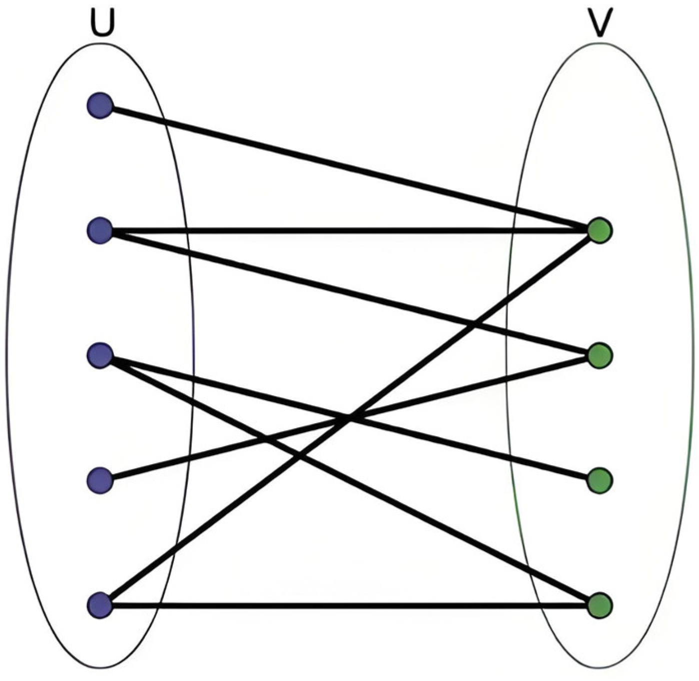
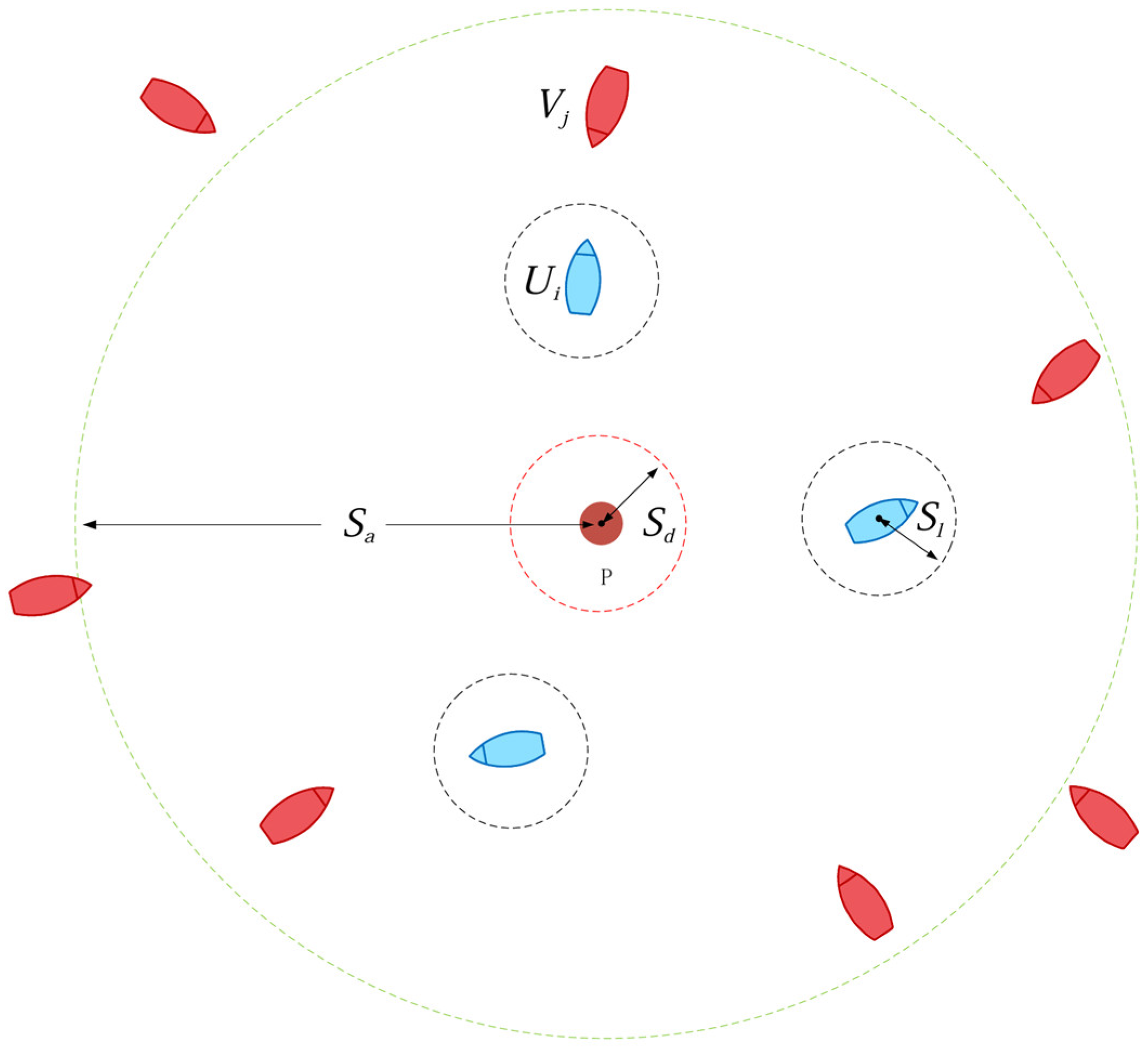
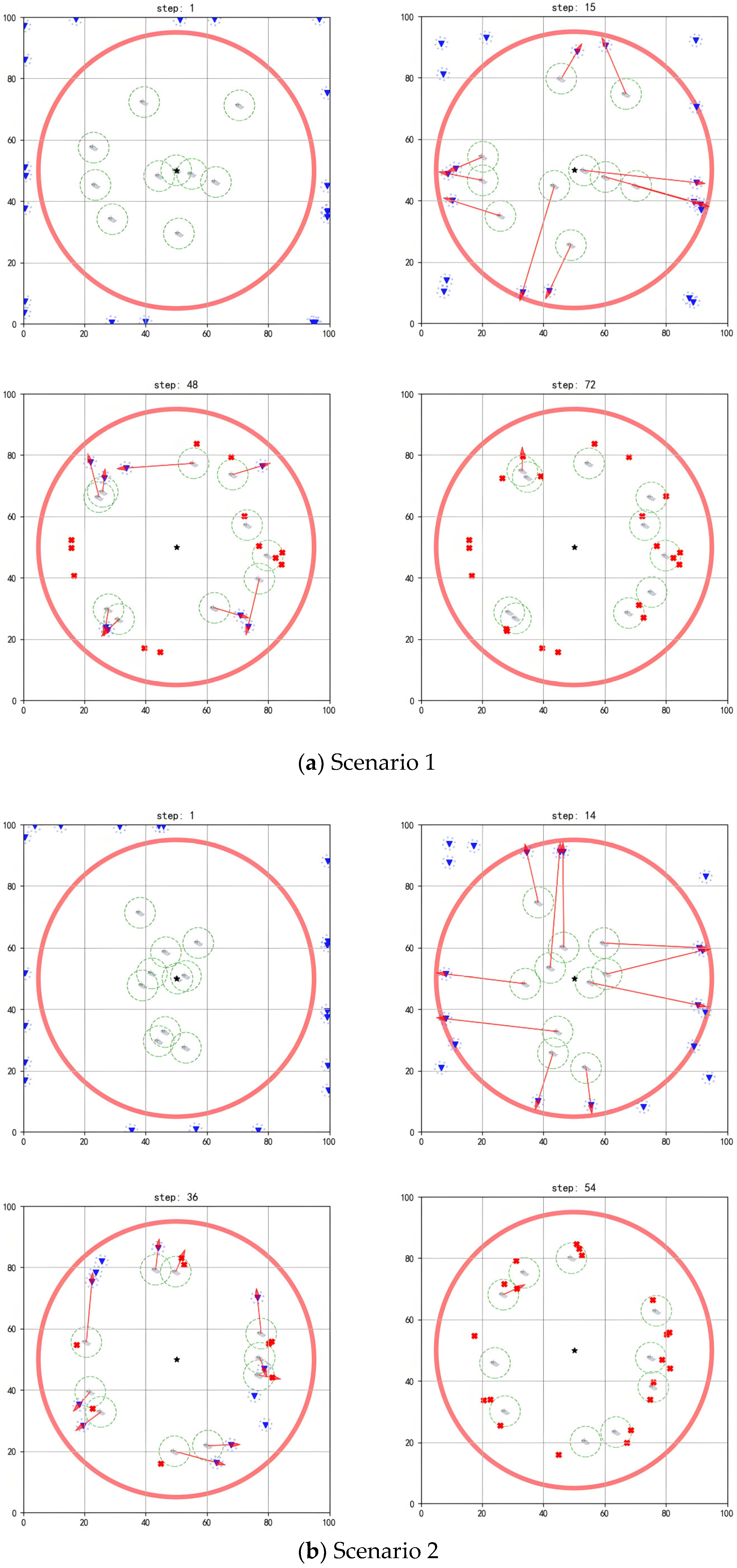
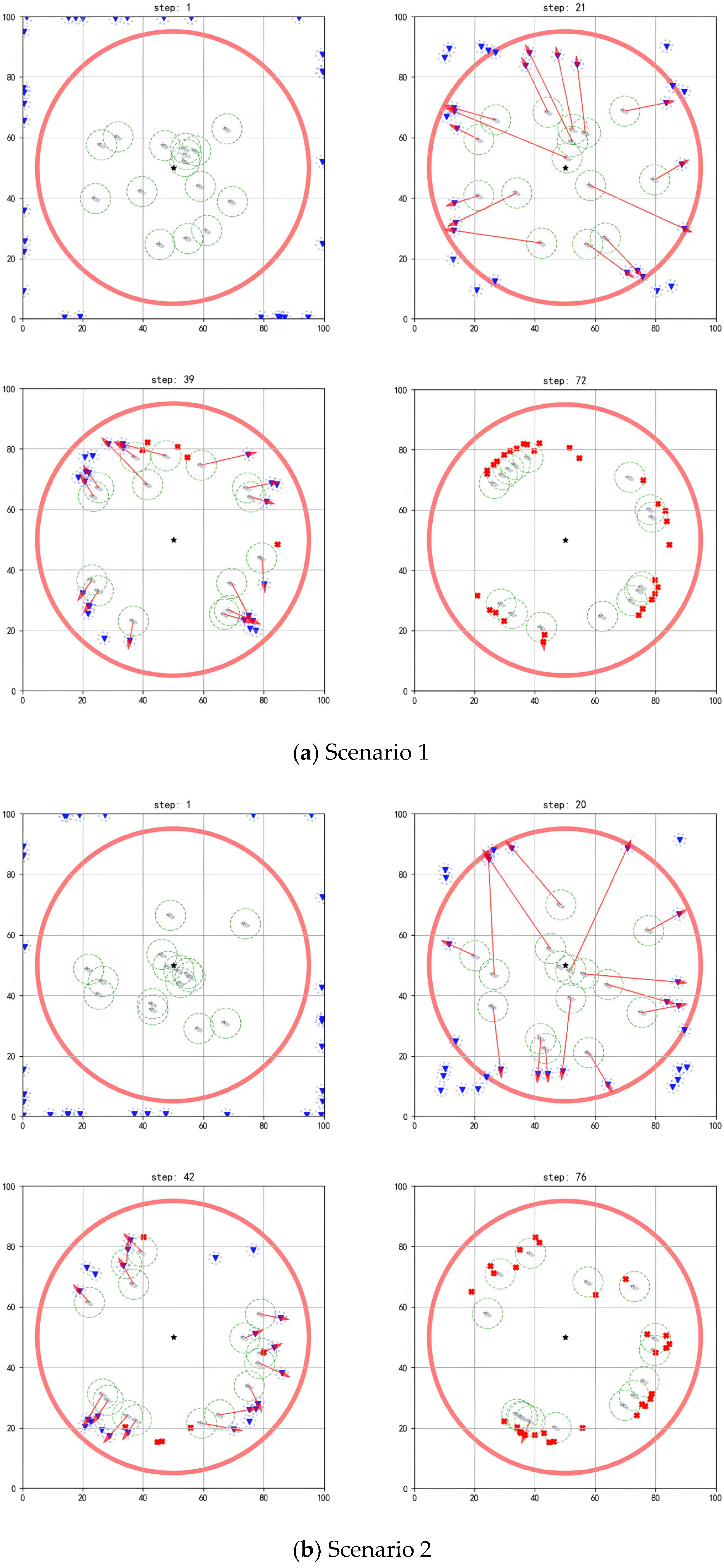
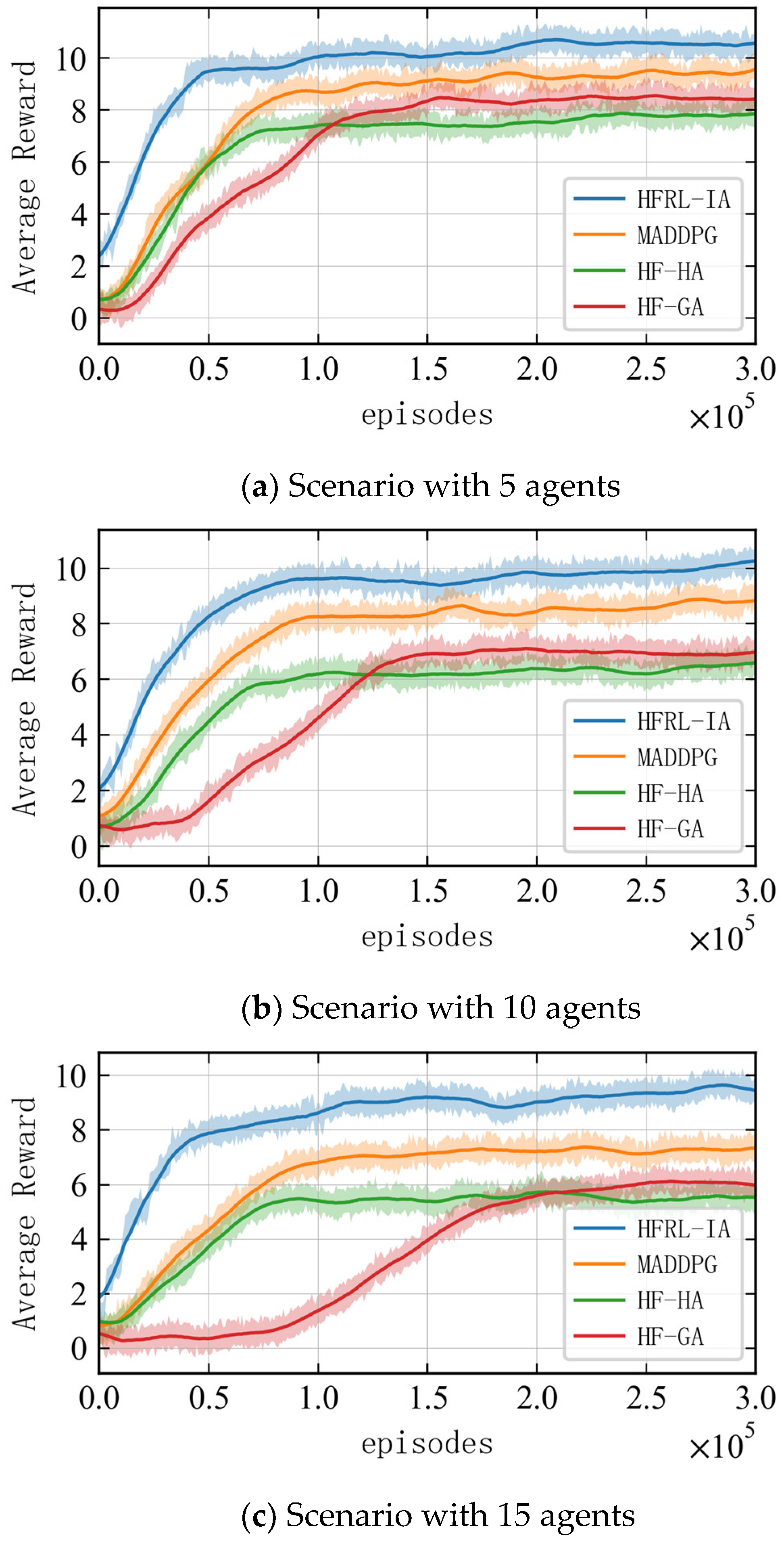
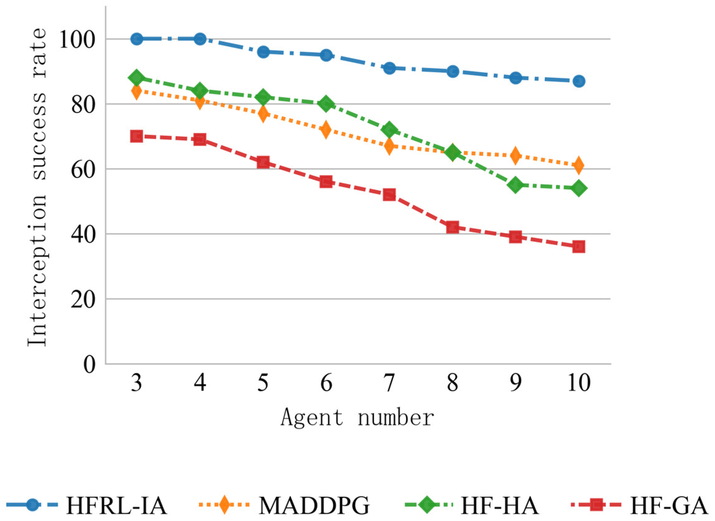
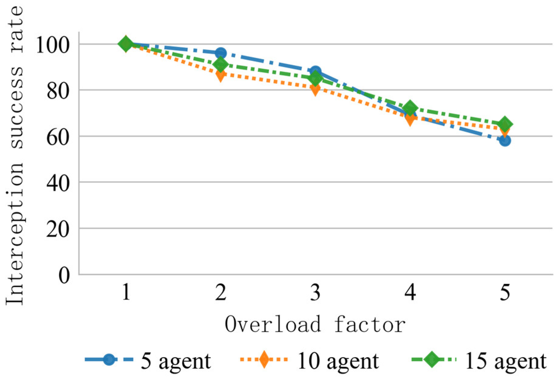
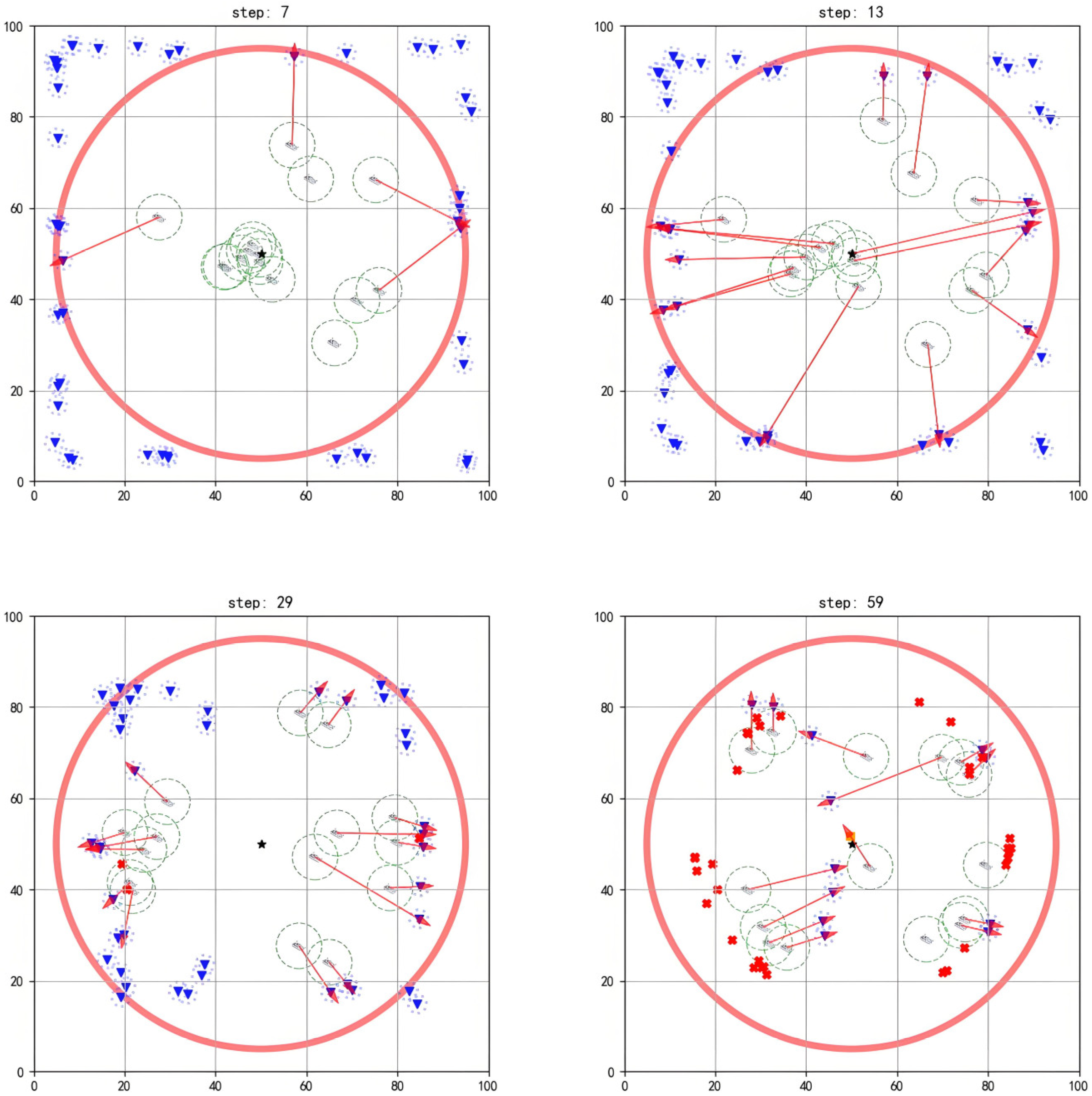
Disclaimer/Publisher’s Note: The statements, opinions and data contained in all publications are solely those of the individual author(s) and contributor(s) and not of MDPI and/or the editor(s). MDPI and/or the editor(s) disclaim responsibility for any injury to people or property resulting from any ideas, methods, instructions or products referred to in the content. |
© 2025 by the authors. Licensee MDPI, Basel, Switzerland. This article is an open access article distributed under the terms and conditions of the Creative Commons Attribution (CC BY) license (https://creativecommons.org/licenses/by/4.0/).