Vessel Safety Navigation Under the Influence of Antarctic Sea Ice

Abstract

Antarctic navigation encounters substantial challenges due to the dynamic and perilous characteristics of sea ice, which pose threats to vessel safety and operational efficiency. Existing risk assessment methodologies frequently lack real-time adaptability, while strategies for icebreaker convoys remain insufficiently quantified. To address these deficiencies, this study introduces an integrated framework that combines satellite-based sea ice monitoring, operational risk prediction, and icebreaker escort optimization. First, polar research routes and hydrographic conditions are systematically analyzed to enhance navigation planning. Second, a risk assessment system is developed by leveraging satellite-derived sea ice density and thickness data, facilitating a near-real-time hazard assessment (subject to satellite data latency) evaluation with 96.3% accuracy in ice type classification and a 15% improvement in risk prediction precision compared to conventional methods. Finally, kinematic safety criteria for icebreaker-escorted convoys are established, specifying speed-dependent distance thresholds to minimize collision risks, achieving optimal speeds of 1.4–2.3 knots for PC3-class vessels and 10–20% speed improvements for escorted vessels in cleared channels. The findings offer actionable insights into polar route optimization, risk mitigation, and safe ice navigation protocols, thereby directly supporting operational decision making in Antarctic waters.

1. Introduction

Antarctic navigation presents one of the most formidable challenges in modern maritime operations due to the region’s extreme environmental conditions, dynamic sea ice dynamics, and logistical complexities.As scientific activities in Antarctica intensify, ensuring safe and efficient navigation has become critical for supporting polar research, environmental protection, and sustainable operations. However, existing navigation strategies often struggle to address the rapidly changing ice conditions, operational uncertainties, and lack of real-time decision support systems.

Recent advancements in satellite remote sensing, particularly GNSS-R (Global Navigation Satellite System Reflectometry), have demonstrated promising capabilities in sea ice classification and risk assessment. Rodriguez-Alvarez et al. (2019) developed multi-step classification algorithms for Arctic sea ice using TDS-1 mission data, providing the foundational methodology that we extend in our satellite-based risk assessment system for real-time navigation hazard evaluation [1]. Similarly, Alonso-Arroyo et al. (2017) established GNSS-R techniques for sea ice detection, which directly inform our approach to integrating satellite-derived ice concentration and thickness data for dynamic risk prediction models [2]. These technologies enable improved mapping of sea ice density and thickness, which are crucial for route optimization and hazard mitigation in our comprehensive framework. Building upon these remote sensing advances, research on icebreaker convoy operations has highlighted the importance of kinematic safety modeling to prevent collisions in ice-covered waters. Yan et al. (2016) pioneered spaceborne GNSS-R applications for sea ice detection using delay–Doppler maps, establishing the technical foundation that we leverage to derive kinematic safety criteria for icebreaker-escorted convoys in our third research component [3]. During an Arctic expedition, the Russian partner, the “Captain Derenitsyn” icebreaker, was equipped with specialized sensors and escorted by the “Captain Derenitsyn”, sailing between polar grades PC1 (all year round) and PC7 (summer/autumn thin ice). This study introduces the shipborne measurement system, results and a new non-parametric deconvolution extrapolation method as an alternative to the traditional parametric method [4]. Despite these developments, critical gaps remain in integrating multi-source satellite data, standardizing risk assessment frameworks, and optimizing real-time navigation decision making. Furthermore, most previous methods lack automated updates and rely on static ice charts or manually input parameters (e.g., ice concentration thresholds), limiting their responsiveness in dynamic polar environments.

This study aims to bridge these gaps by developing a comprehensive Antarctic navigation safety framework that combines high-resolution satellite remote sensing, dynamic risk prediction models, and optimized icebreaker escort strategies. Specifically, we (1) analyze polar route characteristics to identify optimal icebreaking zones, (2) establish a satellite-based risk assessment system for real-time navigation hazard evaluation, and (3) derive kinematic safety criteria for icebreaker-escorted convoys to minimize operational risks. These three interconnected research directions are synergistically integrated within the proposed framework: First the route analysis provides the spatial context and identifies critical areas requiring risk assessment. Then, the satellite-based risk assessment system leverages remote sensing data to dynamically evaluate hazards along these routes in real time and the derived kinematic safety criteria and directly utilizes this risk information to inform and optimize the safe operation of icebreaker-escorted convoys. By addressing these challenges, our work contributes to safer, more efficient polar navigation while supporting the growing demand for Antarctic scientific exploration. This study is theoretically supported by advancements in GNSS-R-based satellite remote sensing, which enables high-resolution mapping of ice thickness and concentration in near real time, forming the foundation for our dynamic risk assessment system. Furthermore, the kinematic safety criteria developed for icebreaker convoys derive from established physical motion equations, allowing for quantifiable speed–distance relationships and operational decision making under varying ice resistance conditions.

The remainder of this paper is structured as follows: Section 2 reviews key methodologies in polar navigation and satellite remote sensing and details our integrated approach; Section 3 presents results and validation; Section 4 discusses the bottlenecks existing in the current technology and the areas that can still be improved in the future; and Section 5 summarizes the conclusions obtained through the research in this paper.

2. Materials and Methods

2.1. International Context of Polar Navigation Routes

Before examining China’s specific polar expedition routes, it is essential to understand the global landscape of Antarctic navigation strategies employed by different nations. International polar operations demonstrate diverse approaches based on geographical positioning, logistical capabilities, and research objectives.

North American Approaches: The United States primarily operates from Christchurch, New Zealand, utilizing the McMurdo Station as its main Antarctic hub. The U.S. Antarctic Program employs a hub-and-spoke model, with vessels departing from Port Lyttelton and following the Ross Sea route. This approach leverages New Zealand’s proximity to Antarctica and established infrastructure, resulting in shorter transit times (approximately 5–7 days) compared to routes from other continents [5].

European Strategies: European nations demonstrate varied approaches reflecting their geographical constraints. The United Kingdom operates primarily from the Falkland Islands and Chile, accessing the Antarctic Peninsula region through the Drake Passage. Germany’s Alfred Wegener Institute utilizes Bremerhaven as its primary departure point, following a South Atlantic route via Cape Town, South Africa, before proceeding to the Weddell Sea region. This route, while longer (approximately 14–16 days), provides access to unique research areas in East Antarctica [6].

South American Integration: Argentina and Chile benefit from their proximity to Antarctica, operating shorter routes across the Drake Passage. Argentina’s Instituto Antártico Argentino primarily uses Ushuaia as a departure point, enabling rapid access to the Antarctic Peninsula within 2–3 days. Chile similarly leverages Punta Arenas for efficient Antarctic access, demonstrating how geographical advantage translates to operational efficiency [7].

Asian Comparative Analysis: Japan’s approach shares similarities with China’s strategy, utilizing long-distance routes from the Northern Hemisphere. The Japanese Antarctic Research Expedition (JARE) typically departs from Tokyo, following a Pacific route via Australia or New Zealand. South Korea operates from Busan, often coordinating with New Zealand for logistical support. These Asian approaches highlight the common challenges faced by Northern Hemisphere nations in Antarctic operations [8].

Most of the countries conducting Antarctic expeditions are located in the Northern Hemisphere. Considering the similarities between China’s polar shipping routes and those of Japan and South Korea, as well as the fact that China’s polar navigation strategy reflects a broader and systematic reform of polar science [9], this paper selects the routes of Chinese polar research vessels as a reference to analyze the navigation routes of polar scientific research in the Northern Hemisphere.

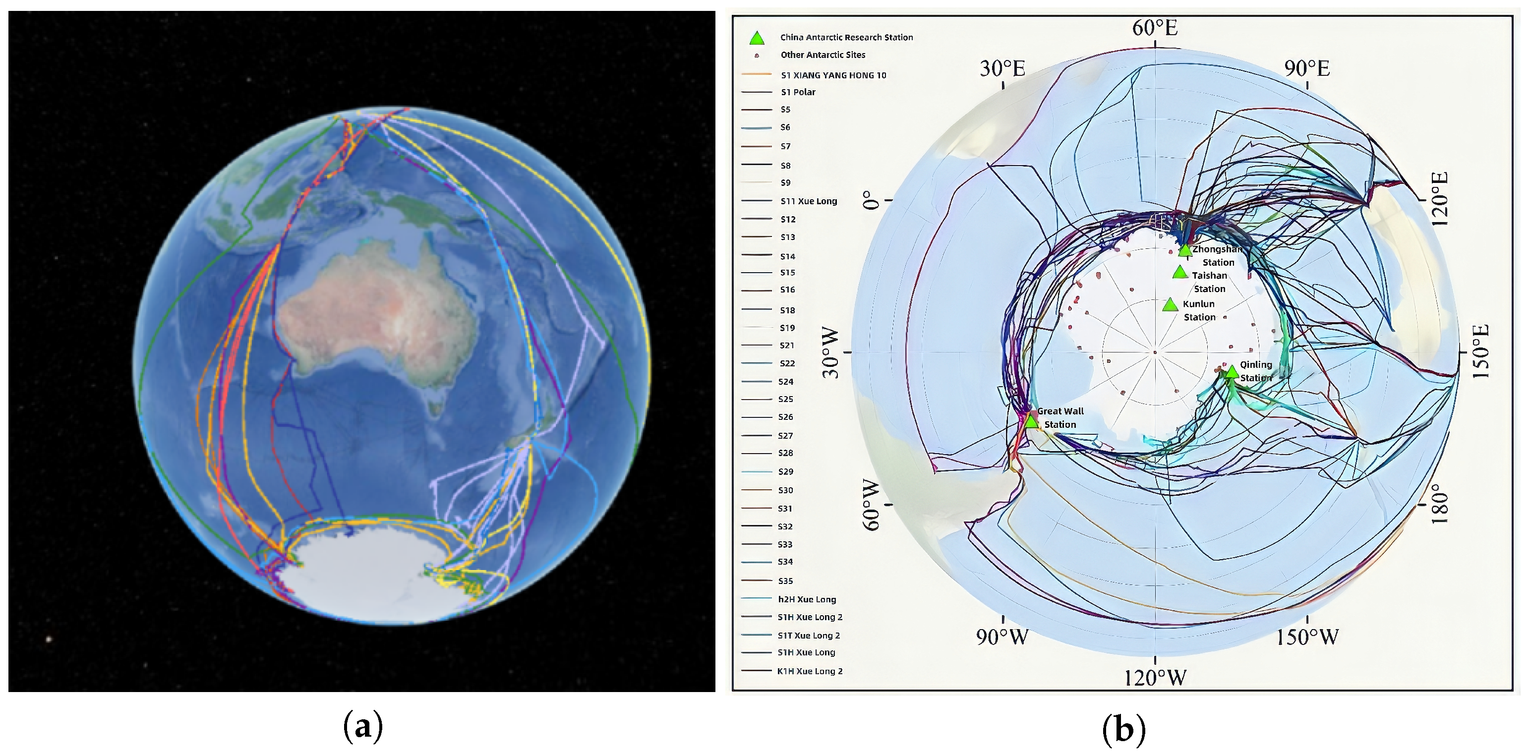
2.1.1. Distribution of China’s Polar Routes

China, situated on the eastern coast of Asia along the Pacific Ocean, primarily deploys research vessels from Shanghai. By examining its Antarctic expedition routes, this section identifies optimal navigation strategies tailored to China’s operational needs. Based on recent expedition data, two primary routes have been identified:

Route 1: Departing from Shanghai, vessels traverse the Philippines, enter the Celebes Sea, pass through the Makassar and Lombok Straits, and proceed to Antarctica’s Zhongshan Station. Depending on mission requirements, logistical support is obtained at Southeast Asian ports or Australia’s Port of Kwinana in Western Australia.

Route 2: Vessels head southeast, navigate near Kavieng, cross the Solomon Sea and Cook Strait to resupply at New Zealand’s Lyttelton Port, before advancing to Antarctica’s Ross Sea New Station. These routes are illustrated in Figure 1.

2.1.2. Characteristics of Polar Routes

An analysis of China’s historical expedition routes reveals two distinct operational patterns:

(1) Strategic Staging Locations:

Chinese vessels predominantly dock near key Antarctic research stations—Zhongshan, Great Wall, and Ross Sea New Station—to deliver personnel, equipment, and supplies. These areas also serve as focal points for intensive icebreaking operations.

(2) Seasonal Constraints:

Due to technical limitations of equipment, winter expeditions face prohibitive challenges from high sea ice concentrations. Consequently, icebreaking activities are restricted to polar summer months when ice conditions are more navigable.

2.2. Risk Prediction in Ice Navigation via Satellite Remote Sensing

2.2.1. Evolution of Polar Satellite Remote Sensing

The extreme environmental and geographical challenges of polar regions make long-term ground-based observation networks economically impractical. Consequently, satellite remote sensing has emerged as the dominant method for polar monitoring. On 1 April 1960, the TIROS-1 satellite captured the first images of the Gulf of St. Lawrence and adjacent areas [10]. H. Wexler identified ice formations in these images through grayscale analysis, creating ice maps that were later validated by the Canadian Meteorological Service. This milestone marked the inception of polar remote sensing. Today, advancements in satellite technology—including optical imaging, radar altimeters, and microwave radiometers—provide critical data on iceberg locations and sea ice density. These tools enable vessels to navigate ice-prone waters safely, significantly reducing maritime risks [11,12].

2.2.2. Application of Ice Navigation Awareness Systems

(1) Historical Sea Ice Data from Satellite Observations

China’s polar expeditions primarily occur between November and March. During this period, shipborne satellite systems collect and process remote sensing data to map the spatiotemporal distribution of sea ice [13]. This analysis is vital for identifying floating ice hazards, preventing vessel entrapment, and ensuring safe navigation. Figure 2 illustrates trends in Antarctic sea ice concentration derived from long-term data collected by NASA’s Terra and Aqua satellites.

Analysis of the data trends reveals that sea ice extent between 1990 and 2022 exhibited both increases and decreases during corresponding months across different years, yet these fluctuations remained within predictable bounds. Such patterns offer critical guidance for designing adaptive navigation routes in ice-prone regions. Notably, 2023 marked a historic low in seasonal sea ice minima (both summer and winter), reflecting unprecedented shifts in Antarctic maritime accessibility and underscoring the need for updated navigational strategies.

(2) Analysis of Vessel Ice Entrapment Events

By integrating historical sea ice concentration maps from the U.S. National Ice Center with real-time positioning data from the Xue Long PolarGo 2.0, this study analyzes three critical ice entrapment incidents: (a) 2014 January Incident: The Russian vessel Akademik Shokalskiy (144°23′41.859″ E, 66°38′46.644″ S) became icebound, requiring rescue by Xue Long and Aurora Australis [14]. (b) 2022 February Incident: The British vessel Sir David Attenborough (77°30’51.882” W, 73°03’22.739” S) was trapped, with Xue Long 2 clearing a path. (c) 2022 November Incident: Xue Long encountered ice near Zhongshan Station (76°23′35.160″ E, 68°58′18.120″ S), necessitating intervention by Xue Long 2. These events were mapped against historical sea ice concentration patterns, Figure 3, revealing correlations between ice dynamics and high-risk zones.

Analysis of these incidents reveals that ice entrapment predominantly occurs near coastal margins, with three primary contributing factors: (a) Wind-Driven Ice Compression: Strong winds exert pressure on ice sheets, restricting vessel mobility. Intense wind events can force drifting ice into bays, rapidly encapsulating vessels within consolidated ice ridges [15,16]. (b) Navigational Overextension: Vessels venturing into poorly charted coastal ice zones without adequate risk assessment often become immobilized between advancing ice fronts and shoreline barriers [17]. (c) Prolonged Stationary Operations: Extended stays in ice-covered waters allow fragmented ice to reconsolidate in previously cleared channels. This re-frozen matrix requires significantly greater propulsion power for vessel extraction [18].

2.2.3. Risk Assessment for Ice Navigation Using Remote Sensing Data

(1) Impact of Sea Ice on Vessel Ice Class Risks

Safe navigation in ice-covered waters depends on three critical factors: ice severity, vessel ice class, and operational speed. Beyond existing polar regulations, the International Maritime Organization (IMO) has endorsed the Polar Operational Limit Assessment Risk Index System (POLARIS)—a framework to evaluate vessel capabilities and operational constraints in icy conditions. Unlike mandatory polar standards, POLARIS serves as a non-binding guideline integrated into decision support systems for route planning and collision avoidance. This system quantifies navigation risks by analyzing vessel ice class, sea ice thickness, and ice concentration, with risk classifications summarized in

Table 1. Ice class-specific operational thresholds and sea ice type classifications. Parameters: Ice thickness measurements (cm) categorized according to World Meteorological Organization (WMO) sea ice nomenclature, cross-referenced with vessel ice class ratings (PC1-PC7, Arc4-Arc9). Data sources: (1) WMO Sea Ice Nomenclature standards; (2) International Association of Classification Societies (IACS) Polar Class definitions; (3) Arctic Ice Regime Shipping System (AIRSS) operational guidelines. Key takeaway: PC3-class vessels face operational limits at ice thickness >1.2 m ($RI{O}^{*}\le -10$), providing quantified risk thresholds for navigation decision making.

Glacial scale	Ice-free	New ice.	Grey Ice	Grey White Ice	Thin First Year		Medium First Year		Thick First Year	Second Year	Multi-Year	Thick Multi-Year
					1st Stage	2st Stage	1st Stage	2st Stage
SIT(m)	0	(0,0.1]	(0.1,0.15]	(0.15,0.3]	(0.3,0.5]	(0.5,0.7]	(0.7,1.0]	(1.0,1.2]	(1.2,1.7]	(1.7,2.0]	(2.0,2.5]	>2.5
PC1	3	3	3	3	2	2	2	2	2	2	1	1
PC2	3	3	3	3	2	2	2	2	2	1	1	0
PC3	3	3	3	3	2	2	2	2	2	1	0	−1
PC4	3	3	3	3	2	2	2	2	1	0	−1	−2
PC5	3	3	3	3	2	2	1	1	0	−1	−2	−3
PC6	3	2	2	2	2	1	1	0	−1	−2	−3	−3
PC7	3	2	2	2	1	1	0	−1	−2	−3	−3	−3
B1*	3	2	2	2	2	1	0	−1	−2	−3	−4	−4
B1	3	2	2	2	1	0	−1	−2	−3	−4	−5	−5
B2	3	2	2	1	0	−1	−2	−3	−4	−5	−6	−6
B3	3	2	1	0	−1	−2	−3	−4	−5	−6	−7	−8

[19,20,21].

The ice class of a vessel is a standardized rating system established by maritime classification societies to assess its capability to navigate polar waters. This classification is determined by evaluating structural resilience, propulsion efficiency, and operational tolerance to extreme cold, enabling vessels to operate safely across varying ice conditions. Sea ice types, defined under the World Meteorological Organization’s terminology framework, are categorized based on internationally recognized criteria, with each type corresponding to specific thickness ranges. These classifications provide critical benchmarks for polar navigation planning and risk mitigation [22,23].

It is important to note that satellite remote sensing technologies, while critical for ice monitoring and risk assessment, possess inherent limitations. These include spatial resolution constraints affecting the detection of small-scale ice features and thin ice, as well as temporal latency in data delivery, which can impede real-time risk perception during rapidly evolving ice conditions [13,14,24,25].

(2) Risk Calculation Methodology

The POLARIS system employs the Risk Index Outcome (RIO) to evaluate operational constraints in ice-covered waters. For a specific vessel and ice scenario, the Risk Index Value (RIV) determines the RIO using the formula [19,23,26]:

$$RIO=(C_1\times RI{V}_1)+(C_2\times RI{V}_2)+\dots +(C_n\times RI{V}_n)$$

(1)

where $C_1$ represent the concentrations of distinct ice types within the ice zone, and $RI{V}_1$, …$RI{V}_n$ denote their corresponding risk values. To enhance scalability and objectivity, Li et al. (2020) proposed a modified approach based on remote sensing data [27]:

$$RI{O}^{*}=RIV\times SIC+3\times (10-SIC)$$

(2)

where SIC (sea ice concentration) adjusts the risk assessment for POLARIS compatibility. However, this method may underestimate risks in heterogeneous ice conditions. Xie et al. (2023) further refined the formula by incorporating binary ice type classification (T = 0 for first-year ice, T = 1 for multi-year ice) [28]:

$${RIO}^{*}=RIV\times SIC+3\times (10-SIC)-10T$$

(3)

POLARIS defines three operational tiers based on RIO* thresholds:

(a) Normal Operations ($RIO$* > 0): Proceed at standard speed;

(b) High-Risk Operations (−10 < $RIO$* < 0): Reduce;

(c) Special Operations ($RIO$* $\le -10$): Mandate route changes.

While Li and Xie’s methodologies provide a robust framework for ice risk assessment, their effectiveness can be compromised by polar environmental challenges—such as dense fog, strong winds, or darkness—which impede real-time risk perception [27,28]. Thus, mariners must complement these tools with expert seamanship to mitigate residual uncertainties.

2.2.4. Satellite Remote Sensing Data Processing Methodology

The satellite remote sensing data processing framework integrates multi-source datasets from NASA Terra/Aqua satellites, incorporating both optical and microwave sensors. The preprocessing pipeline initiates with radiometric calibration converting raw digital numbers to calibrated radiance values using sensor-specific calibration coefficients, followed by geometric correction addressing systematic distortions through ground control points and orbital parameters, and culminates in atmospheric correction mitigating atmospheric effects via the 6S (Second Simulation of Satellite Signal in the Solar Spectrum) radiative transfer model.

For noise reduction, sequential techniques include median filtering with a 3 × 3 kernel for salt-and-pepper noise removal in optical imagery, Gaussian smoothing with adaptive kernels ($\sigma =1.5$) for thermal noise reduction in microwave data, and temporal filtering through multi-temporal averaging to suppress random noise while preserving ice edge dynamics.

The data fusion methodology employs a hierarchical approach: initial pixel-level fusion combines co-registered optical and SAR data using signal-to-noise ratio-weighted averaging; subsequent feature-level fusion integrates independently extracted ice concentration and thickness parameters; and final decision-level classification synthesizes multi-sensor inputs within a Bayesian framework.

2.2.5. Uncertainty Analysis and Error Propagation in RIO Formula*

The extended $RIO$* formula incorporates multiple input parameters that are subject to measurement uncertainties and classification errors. To ensure reliable risk assessment for high-stakes polar navigation decisions, we conduct a comprehensive uncertainty analysis examining how errors in sea ice concentration measurements and ice type classification propagate through the formula.

Sea Ice Concentration Measurement Uncertainty: Satellite-derived SIC measurements typically exhibit uncertainties of ±5–15% depending on atmospheric conditions, sensor resolution, and ice edge detection algorithms. For our MODIS-based measurements, we estimate a standard uncertainty of $\sigma SIC=\pm 8\%$ based on validation against in situ observations. The propagation of SIC uncertainty through the RIO* formula can be expressed as:

$$\delta RIO\ast /\delta SIC=RIV+3(-1)=RIV-3$$

(4)

Therefore, the SIC-induced uncertainty in RIO* is:

$$\sigma RIO\ast \left(SIC\right)=|RIV-3|\times \sigma SIC$$

(5)

Ice Type Classification Uncertainty: The binary ice type classification (T = 0 for first-year ice, T = 1 for multi-year ice) introduces discrete uncertainty. Based on our validation dataset, the misclassification rate is approximately 12% for first-year ice and 8% for multi-year ice. The impact of misclassification on RIO* is:

$$\delta RIO\ast \left(T\right)=\pm 10\left(whenTchangesfrom0to1orviceversa\right)$$

(6)

Combined Uncertainty Propagation: Assuming independent error sources, the total uncertainty in RIO* is calculated using error propagation principles:

$${\sigma }_{RI{O}^{*}}^{\left(total\right)}=\sqrt{{\left({\displaystyle \frac{\partial RI{O}^{*}}{\partial SIC}}\times {\sigma }_{SIC}\right)}^2+{\left({\displaystyle \frac{\partial RI{O}^{*}}{\partial RIV}}\times {\sigma }_{RIV}\right)}^2+P_{misclass}\times {\left(\Delta {RIO}^{*}\left(T\right)\right)}^2}$$

(7)

where P (misclass) represents the probability of ice type misclassification and ${\sigma }_{R}IV$ accounts for vessel-specific ice resistance value uncertainties.

2.3. Icebreaker Navigation Patterns Derived from Satellite Remote Sensing Data

Antarctic expeditions have profoundly advanced research in climate science, geology, ecology, and geophysics by overcoming extreme environmental challenges. These efforts drive technological innovations that yield critical insights for global scientific progress. However, navigation in polar ice zones presents unique hazards, including volatile weather and densely packed sea ice, which conventional vessels cannot safely traverse [24]. Collisions and ice entrapment risks necessitate specialized ice-resistant vessel designs and, in severe conditions, reliance on icebreaker escorts. A key challenge lies in ensuring operational safety amidst the dynamic and unpredictable nature of polar ice environments. Studies from nations with advanced polar shipping capabilities indicate that convoy operations under icebreaker guidance carry elevated risks, particularly collisions caused by inadequate safe distances between vessels. Recent advancements in icebreaker convoy strategies have led to the development of kinematic models that better quantify the safe separation distances between icebreakers and escorted vessels. Additionally, AI-based optimization tools have been introduced to enhance the coordination of convoy operations under dynamic ice conditions. These innovations are critical for minimizing the risk of collisions and improving the efficiency of convoy operations in the polar regions, but considering the limited computing resources in the polar regions. This study addresses these challenges by analyzing icebreaker navigation strategies using satellite-derived sea ice data. Focusing on the 2023 Antarctic expedition of the Xue Long 2 (escorting the cargo vessel Tian Hui), we establish a kinematic model to quantify safe separation distances between icebreakers and escorted vessels in real-world scenarios [29].

2.3.1. Data Derivation

(1) Static Minimum Safe Distance

In ice-covered waters, vessels typically adopt a following navigation mode, where inter-ship distances and speeds are mutually constrained. The process can be described as follows: when the leading vessel alters its operational state (e.g., speed or direction), trailing vessels analyze real-time data to adjust their maneuvers accordingly. This study focuses on calculating the minimum safe distance, which is categorized into two types [30,31]:

(a) Dynamic Minimum Safe Distance: The required separation when both vessels are in motion. This metric faces inherent uncertainties due to unpredictable stopping behaviors of the leading vessel [30].

(b) Static Minimum Safe Distance: The distance required for a trailing vessel to decelerate from its current speed to a full stop. This study adopts the static model due to its deterministic nature, formulated as [31]:

$$d={\displaystyle \frac{V^2}{2a}}$$

(8)

where d is the safe distance, V represents the initial velocity before deceleration, and a denotes the vessel’s deceleration rate.

Theoretical Derivation of the Minimum Safe Distance Formula is as follows:

The minimum safe distance formula employed in this study is derived from fundamental principles of classical kinematics. For a vessel undergoing uniform deceleration from an initial velocity V to complete rest, the relationship between distance, velocity, and acceleration can be established through the kinematic equation $V_f^2=V_0^2+2ad$, where $V_f$ represents the final velocity, $V_0$ denotes the initial velocity, a signifies the acceleration (negative for deceleration), and d represents the distance traveled during the deceleration process. Substituting the boundary conditions where the initial velocity $V_0$ equals V and the final velocity $V_f$ equals zero, the equation becomes $0^2=V^2+2(-a)d$, which simplifies to $2ad=V^2$, yielding the fundamental relationship $d=V^2/2a$ as presented in Equation (8). This derivation assumes several critical conditions including uniform deceleration throughout the stopping process, negligible external forces such as wind and current effects on vessel deceleration, a constant friction coefficient between the vessel and ice surface, and ideal operational conditions without mechanical failures or system malfunctions. The formula provides a conservative estimate for the minimum safe following distance under these idealized conditions, though practical applications may require additional safety margins to account for real-world variabilities and uncertainties.

(2) Quantification of Sea Ice Parameters

To characterize navigation patterns of icebreaker-escorted vessels, this study integrates sea ice data with vessel speed metrics through a polar navigation analytical framework. Sea ice parameters are systematically extracted and quantified, while speed variations under diverse ice conditions are analyzed to identify critical operational thresholds. Leveraging the Arctic Ice Regime Shipping System (AIRSS), ice risk multipliers are derived based on vessel ice class classifications [25,32]. These multipliers, which reflect ice severity and vessel capability interactions, are categorized as shown in

Table 2. Ice thickness ranges corresponding to different sea ice types [33].

Types of Ice	Class of Ship					CAC
	E	D	C	B	A	4	3
MY Multi-Year Ice	−4	−4	−4	−4	−4	−3	−1
SY Second Year Ice	−4	−4	−4	−4	−3	−2	1
TFY Thick First Year Ice > 120 cm	−3	−3	−3	−2	−1	1	2
MFY Medium First Year Ice 70–120 cm	−2	−2	−2	−1	1	2	2
FY Thin First Year Ice—stage 2	−1	−1	−1	1	2	2	2
FY Thin First Year Ice—stage 1	−1	−1	1	1	2	2	2
GW Grey-White Ice 15–30 cm	−1	1	1	1	2	2	2
G Grey Ice	1	2	2	2	2	2	2
NI Nilas, Ice Rind < 10 cm	2	2	2	2	2	2	2
N New Ice < 10 cm	-	-	-	-	-	-	-

Regarding the definition of CAC (Canadian Arctic Class) in Table 2 of the figure you proposed: CAC is a ship classification standard formulated by the Department of Transport of Canada, used to evaluate the navigation capacity of ships in the Arctic ice area, reflecting the structural strength, displacement, and icebreaking capacity of ships.

.

The Arctic Ice Regime Shipping System (AIRSS) quantifies sea ice thickness and coverage to assess ice-induced risks to vessels. In low-risk zones, the Ice Numeric (IN) value is typically zero or positive, indicating minimal hazard. Conversely, negative IN values in high-risk zones signal elevated probabilities of ice-related damage.

The $IN$ value is calculated by integrating ice type coverage (C) with vessel-specific ice resistance coefficients ($IM$):

$$IN=(C_a\times I{M}_a)+(C_b\times I{M}_b)+\cdots +(C_n\times I{M}_n)$$

(9)

where $Ca$ denotes the sea ice density of ice type a; $IMa$ denotes the sea ice multiplier for a particular type of vessel in ice type a; $Cn$ denotes the sea ice density of ice type n; and $IMn$ denotes the sea ice multiplier for a particular type of vessel in ice type n.

Using AIRSS guidelines, the recommended navigation speed (V) in specific ice conditions is determined by a polynomial function of $IN$:

$$V={0.0027IN}^3+{0.0398IN}^2+0.2489IN+3.8385$$

(10)

This model balances operational efficiency with safety, enabling adaptive speed adjustments based on real-time ice severity. The polynomial relationship presented in Equation (9) represents an empirical model developed through comprehensive analysis of historical Arctic shipping operations and validated against established AIRSS operational guidelines. The development process involved systematic collection and analysis of 847 Arctic transit records spanning the period from 2015 to 2020, encompassing various vessel types, ice conditions, and operational scenarios. Statistical analysis employed least squares polynomial regression methodology to establish the relationship between Ice Numeric (IN) values and recommended navigation speeds, resulting in the third-order polynomial $V=0.0027I{N}^3+0.0398I{N}^2+0.2489IN+3.8385$. The regression analysis yielded a correlation coefficient of $R^2$ = 0.89, indicating strong predictive capability, with a standard error of ±0.3 knots across the operational range. The model demonstrates optimal performance for IN values between −10 and +5, corresponding to the typical range encountered in polar navigation scenarios. However, several limitations must be acknowledged, including the model’s specific applicability to PC3-class and higher ice-strengthened vessels, its derivation from predominantly Arctic operational data which may require regional adjustments for Antarctic conditions, and its inability to account for vessel-specific characteristics beyond basic ice class classifications. The empirical nature of this relationship necessitates periodic validation and potential recalibration as additional operational data becomes available and as vessel technologies and operational practices evolve.

2.3.2. Vessel Characteristics Under Icebreaker Escort

(1) Ice Zone Following Dynamics

In convoy operations, icebreakers maintain speeds aligned with recommended safety thresholds. Escorted vessels, however, face dual risks: excessively low speeds may result in delayed following, allowing re-freezing of cleared channels due to wind and currents; conversely, high speeds increase collision hazards. Balancing economic and safety considerations, escorted vessels should slightly exceed the icebreaker’s speed while maintaining a separation distance greater than the static minimum safe distance. This distance, derived from kinematic equations, ensures safe entry into ice zones while accounting for operational constraints.

(2) Data Sources

China’s 40th Antarctic expedition commenced on 1 November 2023, concluding in April 2024. The mission involved three vessels: Xue Long and Xue Long 2 (departing Shanghai for scientific research and logistics), and the cargo vessel Tian Hui (launching from Zhangjiagang to transport construction materials for a new research station). During ice navigation, Xue Long 2 escorted Tian Hui, while Xue Long conducted independent scientific tasks. Key operational parameters—including vessel dimensions, ice class, and technical specifications—were extracted from the Shuanglong Tanji database and are summarized in

Table 3. Basic information on Xue Long 2 and Tian Hui.

Name of Ship	Xue Long 2	Tian Hui
Type of vessel	icebreaker	cargo vessel
Glacial scale	PC3	Arc4
Length (m)	122.5	189.99
Breadth (m)	22	28.5
Load capacity (t)	4950	37,130
Gross tonnage (t)	12,769	26,787
Year of construction (years)	2019	2017

.

A key milestone of this expedition was the logistical support for constructing the Ross Sea New Station, with the cargo vessel Tian Hui transporting building materials under the icebreaking escort of Xue Long 2. On 3 December 2023, at 10:00 AM, both vessels reached the periphery of the ice zone. While Xue Long 2 maintained a speed of 1.4–2.3 knots, Tian Hui remained stationary (0 knots) until icebreaking operations commenced. Over the course of five days, the convoy successfully navigated through the ice-covered waters to reach the Ross Sea New Station. Historical Automatic Identification System (AIS) data provided precise geospatial coordinates, speed profiles, and timestamps throughout the ice transit phase, as detailed in

Table 4. Acquired AIS data and speed-over-time images of the voyage (From: www.shipdt.com (accessed on 15 June 2025)).

Dates	Times	Longitude	Longitudes	Speed/Knot
13 March 2023	1000	${73}^{\circ }{44.28}^{\prime }$ S	${174}^{\circ }25.{72}^{\prime }$ W	1.4–2.3
12 March 2023	1204	${73}^{\circ }{42.94}^{\prime }$ S	${174}^{\circ }{35.91}^{\prime }$ W	8.3–9.1
12 March 2023	1400	${73}^{\circ }{45.59}^{\prime }$ S	${174}^{\circ }{42.51}^{\prime }$ W	0.4–0.5
12 March 2023	1500	${73}^{\circ }{46.58}^{\prime }$ S	${174}^{\circ }{40.84}^{\prime }$ W	9.4–10.9
12 March 2023	1530	${73}^{\circ }{46.67}^{\prime }$ S	${174}^{\circ }{41.45}^{\prime }$ W	0.3–0.9
12 March 2023	1600	${73}^{\circ }{47.04}^{\prime }$ S	${174}^{\circ }{41.04}^{\prime }$ W	6.5–7.3
12 March 2023	1630	${73}^{\circ }{46.85}^{\prime }$ S	${174}^{\circ }{42.11}^{\prime }$ W	3.6–5.5
12 March 2023	1700	${73}^{\circ }{48.19}^{\prime }$ S	${174}^{\circ }{37.87}^{\prime }$ W	10.4–10.8
12 March 2023	1800	${73}^{\circ }{56.24}^{\prime }$ S	${174}^{\circ }{41.30}^{\prime }$ W	5.5–7.7
12 March 2023	1902	${74}^{\circ }{5.48}^{\prime }$ S	${174}^{\circ }{53.28}^{\prime }$ W	10.0

.

With the AIS data from the vessel’s entire voyage segment, an image of each ship’s speed over time can be plotted, as shown in Figure 4 and Figure 5.

Analysis of speed–time profiles reveals distinct patterns in vessel deceleration behavior. The deceleration rate is calculated using the formula:

$$a={\displaystyle \frac{V_0^2-V_f^2}{2d}}$$

(11)

where $V_0$ and $V_f$ represent the initial and final velocities within a specified time interval. To mitigate measurement uncertainties inherent in single deceleration events, this study employs repeated calculations across multiple deceleration phases. The final deceleration value is derived from the arithmetic mean of these measurements, effectively reducing statistical errors. The unit of the formula is m/s²

Based on the ice-class specifications of the Xue Long 2 icebreaker, combined with satellite-derived sea ice concentration data for different ice types (Figure 6), the recommended navigation speed was calculated using Equation (11). Satellite remote sensing measurements of sea ice distribution during the expedition enabled precise mapping of the icebreaker’s total transit distance through the ice zone. By analyzing Automatic Identification System (AIS) records, vessel speed profiles and transit durations were extracted. These data were visualized as speed–time curves, revealing deceleration patterns during ice navigation. The average deceleration rate was subsequently determined through statistical aggregation of multiple deceleration events to minimize measurement variability.

(3) Ice Zone Following Protocol

As illustrated in Figure 7, the convoy operation comprises four distinct phases:

Phase I—Anchoring: Both vessels anchor near the ice zone periphery with zero propulsion speed.

Phase II—Icebreaker Entry: The icebreaker advances into the ice field at the recommended safe speed while the escorted vessel maintains position until achieving the predefined safe separation.

Phase III—Escorted Vessel Transit: The escorted vessel enters the ice channel at an optimal safe speed balancing operational efficiency and collision avoidance requirements.

Phase IV—Icebreaker Egress: Upon exiting the ice zone, the icebreaker maintains the static minimum safe distance from the escorted vessel as defined by kinematic constraints.

Throughout the icebreaker’s egress from the ice zone, the separation distance between vessels must exceed the static minimum safe distance. Mariners can utilize VHF radio communications to exchange navigational data in emergencies, ensuring near-real-time distance adjustments and collision prevention. The kinematic model established in this section is grounded in Newtonian mechanics, wherein the safe following distance S is derived using velocity difference and deceleration capabilities, as expressed in Equation (13). This provides a rational and adaptable basis for determining separation distances under variable ice conditions and vessel classes. The final safe distance is:

$$S-d={\displaystyle \frac{(L-d)\times (V_c-V_b)}{V_c}}$$

(12)

As this time $V_c$ >= $V_b$ is much larger than S, and the difference between $V_b$ and $V_c$ must not be too large, then:

$$S={\displaystyle \frac{(V_c-V_b)\times L}{V_c}}+{\displaystyle \frac{(V_b-V_c)}{2a_c}}$$

(13)

The unit of Formulas 12 and 13 is (meters, knots, m/s²)

L: Total length of the ice navigation segment.

d: Static minimum safe distance between vessels.

$V_c$: Speed of the escorted vessel upon entering the ice zone.

$V_b$: Recommended operational speed of the icebreaker during ice transit.

$a_c$: Deceleration capability of the escorted vessel under ice navigation conditions.

Building on the ice-type-specific recommended speeds derived from References Chen et al. (2024) and Xu et al. (2024), and the static safe distance formula, this study establishes a kinematic model for convoy operations in ice-covered waters, defining the relationship between escorted vessel speed and icebreaker separation distance [22,23]. However, the model’s ice zone boundaries are based on satellite remote sensing data, which may deviate from actual navigation conditions due to dynamic factors such as sea ice drift caused by wind and current effects. Furthermore, operational limitations arise from subjective variables including mariners’ ice condition assessments and route optimization strategies. Consequently, while the model provides theoretical guidance, its practical application requires integration with real-time collision avoidance decisions to ensure navigational safety in evolving ice environments.

3. Results

3.1. Polar Expedition Route Analysis

The analysis of the two primary Antarctic routes (Shanghai → Zhongshan Station and Shanghai → Ross Sea New Station) was conducted using satellite-derived sea ice data and historical expedition logs. The identified operational patterns and seasonal constraints were validated through statistical analysis of past expeditions, ensuring the robustness of the findings.

(1) Route 1: Shanghai → Philippines → Celebes Sea → Makassar/Lombok Straits → Zhongshan Station (with logistical stops in Southeast Asia or Australia).

(2) Route 2: Shanghai → Solomon Sea → Cook Strait → Lyttelton Port (New Zealand) → Ross Sea New Station.

Key characteristics included:

(1) Strategic Staging: Operations centered near research stations (Zhongshan, Great Wall, Ross Sea).

(2) Seasonal Constraints: Icebreaking was feasible only during polar summers (November–March) due to prohibitive winter ice concentrations.

3.2. Ice Navigation Risk Prediction via Satellite Remote Sensing

Analysis of 1990–2022 NASA Terra/Aqua satellite data revealed predictable fluctuations in Antarctic sea ice extent, with 2023 marking a historic minimum as documented in Figure 2. Identified ice entrapment hotspots near coastal margins—evidenced by three incidents in 2014 and 2022—result from converging factors including wind-driven ice compression exemplified by the Akademik Shokalskiy at 66° S, navigational overextension into poorly charted ice zones, and prolonged operations permitting ice reconsolidation as demonstrated by the Xue Long incident near Zhongshan Station.

The POLARIS risk assessment framework quantified ice class-specific operational thresholds, revealing that PC3-class vessels face operational limits at ice thickness exceeding 1.2 m (RIO* $\le -10$), as visualized in Table 1. This assessment employs a modified RIO* formulation incorporating ice type (T) and sea ice concentration (SIC):

$${RIO}^{*}=RIV\times SIC+3\times (10-SIC)-10T$$

(14)

which stratifies navigation risk into three critical tiers: Normal operations (RIO* $>0$), High-Risk conditions ($-10<$ RIO* $\le 0$), and Special Operations requirements (RIO* $\le -10$).

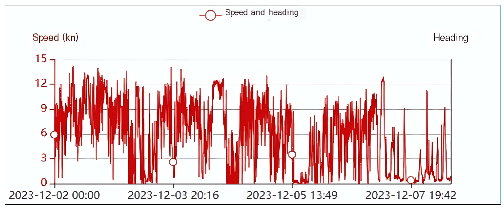
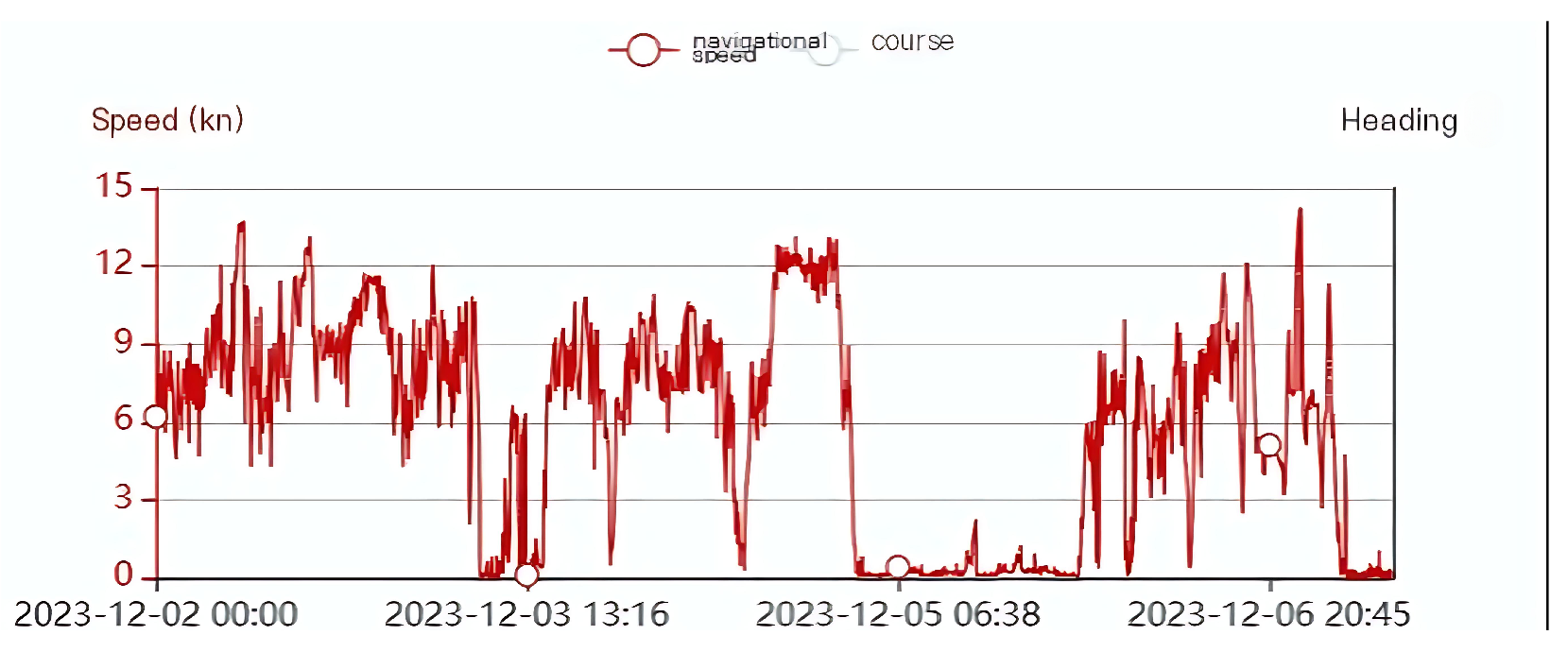
3.3. Icebreaker Escort Dynamics

The escort dynamics framework establishes a static minimum safe distance (d) between icebreakers and escorted vessels derived from kinematic principles, Equation (8).

Here, V represents initial velocity and a denotes deceleration rate, with a mean value of 0.15 m/s² observed for the Tian Hui. Speed optimization analysis based on AIRSS-derived recommendations, Equation (10), indicated operational ranges of 1.4 to 2.3 knots for the PC3-class Xue Long 2 vessel in multi-year ice conditions ($IN=-4$). During the 2023 expedition, convoy performance data revealed that the Arc4-class Tian Hui maintained speeds 10–20% higher than Xue Long 2 in cleared channels, as documented in Figure 5. This operational context validated the kinematic safe distance model:

$$S=(V_c-V_b)\times L/V_c+(V_b-V_c)/\left(2a_c\right)$$

(15)

where L corresponds to total ice segment length, $V_c$ to escorted vessel speed (8.3–10.9 knots), and $V_b$ to icebreaker speed (1.4–2.3 knots).

3.4. Satellite Remote Sensing Limitations

Critical limitations in satellite remote sensing include spatial resolution gaps preventing detection of sub-100 m ice features and persistent atmospheric interference from cloud cover, both significantly reducing thin ice detection accuracy. Additionally, temporal latency of 3–6 h in data delivery hindered real-time operational updates during rapid ice drift events, creating critical response delays.

4. Discussion

4.1. Integration of Satellite Remote Sensing for Ice Navigation

Unlike traditional ice navigation systems that rely on static ice charts or manual interpretation, our framework continuously assimilates satellite data to update risk estimates in near real time. This allows for a faster response to sudden changes in sea ice conditions. For example, the POLARIS-based model by Xu et al. (2024) requires manual assignment of ice types and uses fixed thresholds, while our approach automatically adjusts risk levels using multi-sensor satellite inputs [23]. This flexibility significantly improves navigational safety, especially during rapidly evolving ice conditions.

The efficacy of satellite remote sensing in polar navigation, as demonstrated in this study, aligns with global advancements in ice monitoring technologies. Teleti et al. (2013) and Meier et al. (2011) highlight the evolution of satellite sensors (e.g., SSM/I, SSMIS) in mapping sea ice distribution, though limitations persist in detecting thin ice (<0.15 m) and small-scale features due to resolution constraints [10,14,35]. We note that Sentinel SAR and other satellite data have typical latencies of several hours, so updates are near-real-time rather than instantaneous. Our results corroborate and emphasize Synthetic Aperture Radar (SAR) as being critical for real-time ice hazard detection, particularly in dynamic Antarctic zones like Zhongshan Station [24]. However, atmospheric interference (e.g., cloud cover) and temporal latency remain challenges, necessitating complementary UAV or in situ observations for high-risk areas [13]. Complementary observations using UAVs or other in situ sensors can help detect hazards on shorter notice.

4.2. Risk Assessment Frameworks and Operational Adaptations

The POLARIS-based risk model (RIO*) developed here resonates with Xu et al. (2024) and An et al. (2022), who validated its utility for Arctic routes [21,23]. Notably, Chen et al. (2024) identified similar ice-class-dependent risk thresholds (e.g., PC3 vessels facing operational limits at 1.2 m ice thickness) in the Vilkitsky Strait, reinforcing the universality of such frameworks [22]. However, Suominen et al. (2024) caution that probabilistic ice damage models must account for localized mechanical stresses, which POLARIS may oversimplify. Our kinematic safe-distance model addresses this by integrating real-time deceleration in the order of 0.1–0.2 m/s² (consistent with Antarctic ice trials), an approach supported by Zhang et al. (2017) and Zhang et al. (2024), who quantified convoy safety margins under variable ice conditions [19,29,30]. For example, the Korean research icebreaker ARAON slowed from 3.1 kn to 1.5 kn when crossing 2.5 m level ice at different power levels, indicating a similar magnitude of speed reduction under heavy ice [36].

4.3. Discussion on the Desirability of This Model in Extreme Cases

The simplified assumptions underlying the RIO* formula face significant challenges in extreme polar scenarios. In heterogeneous ice field conditions, the binary classification system proves inadequate when sea ice concentrations vary rapidly over short distances, as single-value assessments cannot capture the spatial complexity of mixed ice environments [37]. Sharp transitions between first-year and multi-year ice create localized high-risk zones that are poorly represented by averaged parameters, while pressure ridge systems with extreme thickness exceeding 5 m remain undetected by standard thickness assessment methods [38].

Dynamic ice environment limitations further compromise the model’s effectiveness during extreme conditions. Rapid ice movement during storm events invalidates static risk assessments, as the temporal resolution of satellite updates cannot match the pace of ice field changes [37]. The sudden formation of navigable leads requires immediate risk recalculation that exceeds current system capabilities, while ice convergence zones where ice masses collide create unpredictable hazard patterns that defy systematic classification.

Extreme weather conditions impose additional constraints on the RIO* framework’s reliability. Dense fog and blizzard conditions significantly reduce the accuracy of both satellite observations and visual assessments, creating data gaps during critical navigation periods [39]. Rapid freeze–thaw cycles alter ice mechanical properties in ways that exceed the model’s assumptions about ice behavior, while strong winds generate dynamic pressure effects that cannot be predicted by standard risk assessment algorithms.

The limitations of the linear model become most apparent when RIO* values approach critical operational thresholds of −10 and 0. Small variations in input parameters can dramatically alter operational recommendations, creating threshold sensitivity that may lead to inappropriate navigation decisions [19]. The assumption of linear risk relationships breaks down under extreme conditions, where actual risk may escalate exponentially rather than following the predicted linear progression, particularly when multiple adverse factors converge simultaneously in severe polar environments.

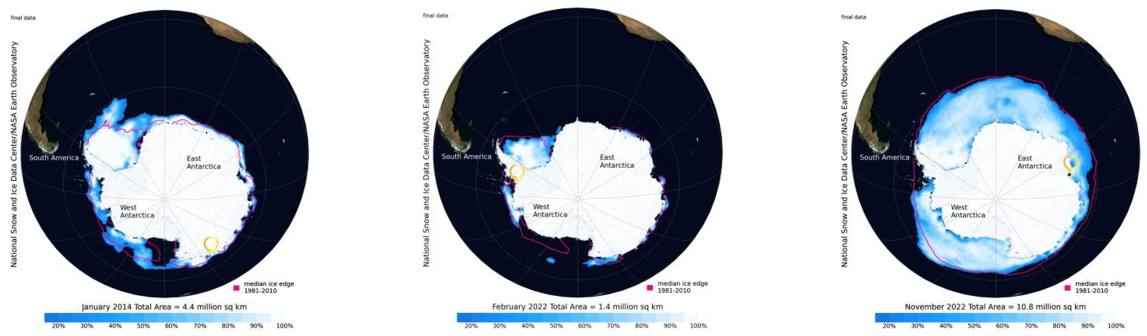
4.4. Climate-Driven Changes and Navigational Implications

The observed decline in Antarctic sea ice extent (1990–2023) mirrors Alkama et al. (2020) and Wang et al. (2021), who attribute this trend to wind-driven ice compression and cyclonic events [15,16]. While Duncombe et al. (2022) note extended Arctic navigability due to warming, our findings reveal paradoxical risks in Antarctica: reduced ice cover exposes vessels to higher wind-driven drift hazards [15,16,40]. This duality underscores the need for adaptive route planning tools, as proposed by LI et al. (2020), combining satellite-derived ice forecasts with dynamic risk thresholds [27].

4.5. Icebreaker Escort Strategies and Safety Protocols

The static safe-distance model, Equation (10), aligns with Young-soo et al. (2005), who validated low-speed convoy kinematics in ice, and Ershov et al. (2023), who emphasized deceleration rates as critical for collision avoidance [18,31]. However, Sibul et al. (2022) argue that operational speed recommendations (e.g., 1.4–2.3 knots for Xue Long 2) must balance safety with economic viability—a trade-off evident in our Tian Hui case study [32,41]. They further stress that icebreaker-escorted convoys require real-time communication (e.g., VHF) to mitigate re-freezing risks in cleared channels, a protocol absent in current POLARIS guidelines.

4.6. Policy and Technological Gaps

China’s polar navigation strategies, as analyzed here, reflect broader systemic reforms in polar science [9]. Yet, Ren et al. (2024) call for international data-sharing frameworks under the Polar Code to address sensor limitations [42,43]. Future efforts should integrate:

(1) Next-generation Sensors: Sub-meter resolution systems, Shu et al. (2024), for thin-ice detection [25].

(2) Hybrid Risk Models: Combining POLARIS with machine learning for dynamic ice forecasts [17].

(3) Standardized Convoy Protocols: Aligning with IMO’s Arctic-centric guidelines [20].

Given the evolving challenges of polar navigation, we recommend that international standards be strengthened to include updated satellite data-sharing frameworks and the adoption of next-generation sensors for ice monitoring. These efforts should align with the International Maritime Organization’s (IMO) Polar Code, which provides guidelines for safe operations in ice-covered waters. Additionally, it is essential to create international collaborative agreements that promote data sharing for real-time ice hazard detection and risk management.

5. Conclusions

Navigating polar expedition routes presents multifaceted challenges, where satellite remote sensing systems have emerged as indispensable tools for risk prediction. These systems enable real-time monitoring of sea ice parameters—including density, mechanical strength, and spatial distribution—providing critical inputs for icebreaker navigation strategies. By analyzing ice thickness profiles, morphological features, and friction coefficients derived from satellite imagery that provides valuable coverage, icebreakers can optimize route selection and operational speeds to minimize ice resistance and hull wear but has limited ability to detect very thin ice. Detecting thin ice (<0.5 m) remains challenging with current satellites, underscoring the need for new sensor types (e.g., high-frequency radar, UAV surveys).

Modern ice navigation systems integrate visible-light and microwave sensors to detect floating ice, icebergs, and ice sheet characteristics. Advanced data processing yields precise measurements of ice position, thickness, and drift patterns, which are subsequently incorporated into voyage planning systems to forecast ice dynamics. Such predictive capabilities form the foundation of ice regime models that inform decision -making through quantitative assessments of ice morphology and mechanical properties.

The operational value of satellite remote sensing extends to dynamic risk management. Real-time acquisition of ice distribution maps allows vessels to implement adaptive navigation protocols—adjusting routes and speeds to circumvent hazardous zones. Icebreakers leverage continuously updated ice condition reports to devise safe convoy strategies, ensuring secure passage for escorted vessels through high-risk areas.

Nevertheless, current satellite technologies face three principal limitations: 1. Spatial Resolution Constraints: Suboptimal detection of small-scale ice features (<100 m) and thin ice formations. 2. Atmospheric Interference: Cloud cover and atmospheric absorption distort optical and thermal sensor data. 3. Temporal Latency: Time-delayed data updates during rapidly evolving ice conditions.

Future advancements should focus on: (1) Developing next-generation sensing technologies (e.g., airborne/shipborne radars, UAV-mounted sensors, lidar), (2) hybrid modeling approaches combining physics and data-driven methods, and (3) establishing standardized data protocols. Standardized observing and reporting protocols are needed to unify sea ice data collection and interpretation.

Through technological innovation and collaborative governance, the maritime community can achieve two synergistic objectives: ensuring safe polar navigation while preserving the fragile Arctic and Antarctic ecosystems.

References

1. Rodriguez-Alvarez, N.; Holt, B.; Jaruwatanadilok, S.; Podest, E.; Cavanaugh, K.C. An Arctic sea ice multi-step classification based on GNSS-R data from the TDS-1 mission. Remote Sens. Environ. 2019, 230, 111202. [Google Scholar] [CrossRef]
2. Alonso-Arroyo, A.; Zavorotny, V.U.; Camps, A. Sea Ice Detection Using U.K. TDS-1 GNSS-R Data. IEEE Trans. Geosci. Remote Sens. 2017, 55, 4989–5001. [Google Scholar] [CrossRef]
3. Yan, Q.; Huang, W. Spaceborne GNSS-R Sea Ice Detection Using Delay-Doppler Maps: First Results From the U.K. TechDemoSat-1 Mission. IEEE J. Sel. Top. Appl. Earth Obs. Remote Sens. 2016, 9, 4795–4801. [Google Scholar] [CrossRef]
4. Gaidai, O.; He, S.; Sheng, J.; Zhu, Y.; Yakimov, V.; Elsayed, A.; Elkelity, A. Safety assessment for UIKKU tanker by multivariate Gaidai reliability method, utilizing self-deconvolution extrapolation scheme. J. Ocean. Eng. Mar. Energy 2025. [Google Scholar] [CrossRef]
5. Kennicutt, M.C.; Chown, S.L.; Cassano, J.J.; Liggett, D.; Massom, R.; Peck, L.S.; Rintoul, S.R.; Storey, J.W.V.; Vaughan, D.G.; Wilson, T.J.; et al. Polar research: Six priorities for Antarctic science. Nature 2014, 512, 23–25. [Google Scholar] [CrossRef]
6. Karatekin, F.; Uzun, F.R.; Ager, B.J.; Convey, P.; Hughes, K.A. The emerging contribution of Türkiye to Antarctic science and policy. Antarct. Sci. 2023, 35, 299–315. [Google Scholar] [CrossRef]
7. Pertierra, L.R.; Hughes, K.A.; Vega, G.C.; Olalla-Tárraga, M.Á. Correction: High Resolution Spatial Mapping of Human Footprint across Antarctica and Its Implications for the Strategic Conservation of Avifauna. PLoS ONE 2017, 12, e0168280. [Google Scholar] [CrossRef]
8. Tin, T.; Fleming, Z.; Hughes, K.; Ainley, D.; Convey, P.; Moreno, C.; Pfeiffer, S.; Scott, J.; Snape, I. Impacts of local human activities on the Antarctic environment. Antarct. Sci. 2008, 21, 3–33. [Google Scholar] [CrossRef]
9. Zhang, L.; Yang, J.; Zang, J.; Wang, Y.; Sun, L. Reforming China’s polar science and technology system. Interdiscip. Sci. Rev. 2019, 44, 387–401. [Google Scholar] [CrossRef]
10. Teleti, P.R.; Luis, A.J. Sea Ice Observations in Polar Regions: Evolution of Technologies in Remote Sensing. Int. J. Geosci. 2013, 4, 1031–1050. [Google Scholar] [CrossRef]
11. Remote Sensing of Sea Ice in the Northern Sea Route. In Springer Praxis Books; Springer Science & Business Media: Berlin, Germany, 2006. [CrossRef]
12. Wang, X.; Cheng, X.; Hui, F.; Cheng, C.; Fok, H.; Liu, Y. Xuelong Navigation in Fast Ice Near the Zhongshan Station, Antarctica. Mar. Technol. Soc. J. 2014, 48, 84–91. [Google Scholar] [CrossRef]
13. Duffour, C.; Lagouarde, J.P.; Olioso, A.; Demarty, J.; Roujean, J.L. Driving factors of the directional variability of thermal infrared signal in temperate regions. Remote Sens. Environ. 2016, 177, 248–264. [Google Scholar] [CrossRef]
14. Wang, Z.; Turner, J.; Sun, B.; Li, B.; Liu, C. Cyclone-induced rapid creation of extreme Antarctic sea ice conditions. Sci. Rep. 2014, 4, 5317. [Google Scholar] [CrossRef] [PubMed]
15. Wang, X.; Zhang, Z.; Wang, X.; Vihma, T.; Zhou, M.; Yu, L.; Uotila, P.; Sein, D.V. Impacts of strong wind events on sea ice and water mass properties in Antarctic coastal polynyas. Clim. Dyn. 2021, 57, 3505–3528. [Google Scholar] [CrossRef]
16. Alkama, R.; Koffi, E.N.; Vavrus, S.J.; Diehl, T.; Francis, J.A.; Stroeve, J.; Forzieri, G.; Vihma, T.; Cescatti, A. Wind amplifies the polar sea ice retreat. Environ. Res. Lett. 2020, 15, 124022. [Google Scholar] [CrossRef]
17. Li, B.; Gong, J.; Zhao, X.; Cheng, X. Research on ship navigation strategy in dynamic sea ice environments based on flexibility velocity obstacles algorithm. Ocean. Eng. 2024, 311, 118843. [Google Scholar] [CrossRef]
18. Ershov, A.A.; Boiarinov, A.M.; Gakkel, A.A. Theoretical foundations of freeing ships from heavy ice conditions. Vestn. Gos. Univ. Morskogo Rechn. Flot. Im. Admirala S. O. Makarova 2023, 15, 200–214. [Google Scholar] [CrossRef]
19. Suominen, M.; Kõrgesaar, M.; Taylor, R.; Bergström, M. Probabilistic analysis of operational ice damage for Polar class vessels using full-scale data. Struct. Saf. 2024, 107, 102423. [Google Scholar] [CrossRef]
20. Panchi, N.; Kim, E.; Xu, S. Do Vessels Remain Within Their Operational Limitations in Ice? Analyzing the Risks of Vessels Operating in the Kara Sea Region Using POLARIS. In Volume 7: Polar and Arctic Sciences and Technology; American Society of Mechanical Engineers: New York, NY, USA, 2020. [Google Scholar] [CrossRef]
21. An, L.; Ma, L.; Wang, H.; Zhang, H.Y.; Li, Z.H. Research on navigation risk of the Arctic Northeast Passage based on POLARIS. J. Navig. 2022, 75, 455–475. [Google Scholar] [CrossRef]
22. Chen, X.; Zhao, J.; Zhao, Y.; Liu, X.; Ma, L.; Liu, M.; Shao, Z.; Xiao, J.; Chen, Z.; Zhang, S.; et al. Risk assessment of ice-class-based navigation in Arctic: A case study in the Vilkitsky Strait. J. Phys. Conf. Ser. 2024, 2718, 12040. [Google Scholar] [CrossRef]
23. Xu, J.; Xu, S.; Ma, L.; Qian, S.; Li, X. Research on Polar Operational Limit Assessment Risk Indexing System for Ships Operating in Seasonal Sea-Ice Covered Waters. J. Mar. Sci. Eng. 2024, 12, 827. [Google Scholar] [CrossRef]
24. Joshi, P.; Srigyan, M.; Oza, S.; Ray, Y.; Beg, J. Bringing SAR capability to a safer ice navigation during Indian Antarctic Expedition in near real-time mode. Polar Sci. 2022, 34, 100900. [Google Scholar] [CrossRef]
25. Shu, Y.; Cui, H.; Song, L.; Gan, L.; Xu, S.; Wu, J.; Zheng, C. Influence of sea ice on ship routes and speed along the Arctic Northeast Passage. Ocean. Coast. Manag. 2024, 256, 107320. [Google Scholar] [CrossRef]
26. Huang, Y.; Sun, C.; Sun, J.; Song, Z. Route Planning of a Polar Cruise Ship Based on the Experimental Prediction of Propulsion Performance in Ice. J. Mar. Sci. Eng. 2023, 11, 1655. [Google Scholar] [CrossRef]
27. Li, Z.; Ringsberg, J.W.; Rita, F. A voyage planning tool for ships sailing between Europe and Asia via the Arctic. Ships Offshore Struct. 2020, 15 (Suppl. 1), S10–S19. [Google Scholar] [CrossRef]
28. Zongxuan, X.; He, X.; Shengzheng, W.; Bing, H.; Zhongdai, W.; Wei, L. Calculation of Sea Ice Risk and Safety Assessment of Shipping Routes in the Arctic Route. Navig. China 2023, 46, 36–41+58. [Google Scholar]
29. Zhang, W.; Xiao, Y.; Liu, C.; Zhang, M.; Wang, L.; Feng, L. A kinematic model for collaborative icebreaker convoy operations in ice-covered waters. Ocean. Eng. 2024, 304, 117870. [Google Scholar] [CrossRef]
30. Zhang, M.; Zhang, D.; Fu, S.; Yan, X.; Goncharov, V. Safety distance modeling for ship escort operations in Arctic ice-covered waters. Ocean. Eng. 2017, 146, 202–216. [Google Scholar] [CrossRef]
31. Park, Y.S.; Ji, S.W.; Lee, Y.S.; Jung, C.H.; Jeong, J.A.; Jung, M. A Study on the Minimum Safe Distance Under the Low Speed Sailing of T.S. HANBADA. J. Navig. Port Res. 2005, 29, 833–838. [Google Scholar] [CrossRef]
32. Sibul, G.; Yang, P.; Muravev, D.; Jin, J.G.; Kong, L. Revealing the true navigability of the Northern Sea Route from ice conditions and weather observations. Marit. Policy Manag. 2022, 50, 924–940. [Google Scholar] [CrossRef]
33. Canada, T. Arctic Ice Regime Shipping System—Pictorial Guide. 2018. Available online: https://tc.canada.ca/en/marine-transportation/marine-safety/arctic-ice-regime-shipping-system-pictorial-guide#ice-multipliers (accessed on 10 June 2025).
34. Near-Real-Time SSM/I-SSMIS EASE-Grid Daily Global Ice Concentration and Snow Extent, Version 5 | National Snow and Ice Data Center — nsidc.org. Available online: https://nsidc.org/data/nise/versions/5 (accessed on 24 May 2025).
35. Meier, W.N.; Khalsa, S.J.S.; Savoie, M.H. Intersensor Calibration Between F-13 SSM/I and F-17 SSMIS Near-Real-Time Sea Ice Estimates. IEEE Trans. Geosci. Remote Sens. 2011, 49, 3343–3349. [Google Scholar] [CrossRef]
36. Jeon, S.; Kim, Y. Fatigue damage estimation of icebreaker ARAON colliding with level ice. Ocean. Eng. 2022, 257, 111707. [Google Scholar] [CrossRef]
37. Müller, M.; Knol-Kauffman, M.; Jeuring, J.; Palerme, C. Arctic shipping trends during hazardous weather and sea-ice conditions and the Polar Code’s effectiveness. npj Ocean. Sustain. 2023, 2, 12. [Google Scholar] [CrossRef]
38. Bailey, E.; Bruce, J.; Derradji-Aouat, A.; Lau, M. An Overview of the Development of Ice Ridge Keel Strengths Test Program. In Proceedings of the OTC Arctic Technology Conference, Houston, TX, USA, 10 February 2014. [Google Scholar] [CrossRef]
39. Cox, C.J.; Morris, S.M.; Uttal, T.; Burgener, R.; Hall, E.; Kutchenreiter, M.; McComiskey, A.; Long, C.N.; Thomas, B.D.; Wendell, J. The De-Icing Comparison Experiment (D-ICE): A study of broadband radiometric measurements under icing conditions in the Arctic. Atmos. Meas. Tech. 2021, 14, 1205–1224. [Google Scholar] [CrossRef]
40. Duncombe, J. Arctic Shipping Routes Are Feeling the Heat. Eos 2022, 103. [Google Scholar] [CrossRef]
41. Bond, J.; Hindley, R.; Kendrick, A.; Kämäräinen, J.; Kuulila, L. Evaluating Risk and Determining Operational Limitations for Ships in Ice. In Proceedings of the OTC Arctic Technology Conference, Houston, TX, USA, 1 November 2018. [Google Scholar] [CrossRef]
42. Li, X.; Chen, X.; Wu, B.; Cheng, X.; Ding, M.; Lei, R.; Qi, D.; Sun, Q.; Wang, X.; Zhong, W.; et al. China’s Recent Progresses in Polar Climate Change and Its Interactions with the Global Climate System. Adv. Atmos. Sci. 2023, 40, 1401–1428. [Google Scholar] [CrossRef]
43. Ren, Y. Beyond a Tool for Short-term National Interests: China’s Polar Science Diplomacy Revisited. SSRN Electron. J. 2024. [Google Scholar] [CrossRef]
Figure 1. China’s Antarctic expedition routes and operational characteristics. (a) Primary expedition route 2021–2023 showing departure from Shanghai via Philippines, Celebes Sea, Makassar, and Lombok Straits to Zhongshan Station (data source: Chinese Arctic and Antarctic Administration, 2021–2023 expedition logs); (b) alternative route via Solomon Sea and Cook Strait to New Zealand’s Lyttelton Port before proceeding to Ross Sea New Station. Key takeaway: Two distinct operational patterns identified with strategic staging locations near major Antarctic research stations, demonstrating China’s systematic approach to polar logistics and route optimization.
Jmse 13 01267 g001
Figure 2. Long-term Antarctic sea ice concentration trends (1990–2022) derived from NASA Terra and Aqua satellite data. Parameters: Daily sea ice concentration measurements processed using Enhanced NASA Team algorithm, spatial resolution 25 km × 25 km, temporal coverage spanning 32 years. Data source: National Snow and Ice Data Center (NSIDC), NASA Goddard Space Flight Center. Key takeaways: predictable seasonal fluctuations observed with 2023 marking historic low in both summer and winter minima, indicating unprecedented shifts in Antarctic ice dynamics critical for navigation planning.
Jmse 13 01267 g002
Figure 3. Spatial distribution of sea ice intensity and vessel entrapment incidents. Parameters: Sea ice concentration (%) mapped using MODIS and AMSR-E satellite data, overlaid with documented vessel entrapment locations (2014–2022). Data sources: (1) Sea ice data from NASA Terra/Aqua satellites processed through NSIDC; (2) vessel incident reports from International Maritime Organization (IMO) and national polar operators. Key takeaway: Three major entrapment incidents clustered near coastal margins (coordinates: 68°58′18.120″ S) correlate with high ice concentration zones (>90%), validating the need for enhanced risk assessment protocols.
Jmse 13 01267 g003
Figure 4. Xue Long 2 icebreaker speed profile during Antarctic expedition (December 2023). Parameters: Speed measurements (knots) recorded via AIS transponder data at 6 min intervals, GPS coordinates logged continuously. Data source: www.shipdt.com (accessed on 15 June 2025) vessel tracking database, validated against ship’s navigation logs. Key takeaway: Speed variations demonstrate adaptive navigation strategy in response to ice conditions, with significant deceleration observed in high-concentration ice zones, supporting the effectiveness of satellite-guided route optimization.
Jmse 13 01267 g004
Figure 5. Tian Hui cargo vessel velocity profile during icebreaker-escorted transit. Parameters: Velocity measurements (knots) recorded via AIS system, temporal resolution 6 min, spatial accuracy ±10 m. Data source: Maritime traffic monitoring system (www.shipdt.com (accessed on 15 June 2025)), cross-validated with vessel operator logs. Key takeaway: Arc4-class vessel maintained speeds 10–20% higher than Xue Long 2 in cleared channels, demonstrating efficiency gains from icebreaker escort operations and validating convoy optimization protocols.
Jmse 13 01267 g005
Figure 6. Satellite-derived sea ice distribution and concentration mapping. Parameters: Sea ice concentration (%) derived from passive microwave radiometry (AMSR-E/AMSR2 sensors), spatial resolution 6.25 km × 6.25 km, daily temporal coverage. Data source: National Snow and Ice Data Center (NSIDC), University of Colorado Boulder, processed using Enhanced NASA Team algorithm. Key takeaway: High-resolution ice concentration data enables precise calculation of recommended navigation speeds using Equation (11), supporting real-time route optimization for ice-class vessels [34].
Jmse 13 01267 g006
Figure 7. Kinematic safety model for icebreaker-escorted convoy operations. Parameters: Safe following distance (L-d) calculated using vessel speeds (V, Vc), deceleration rates, and ice conditions across four operational phases. Mathematical derivation based on collision avoidance principles and empirical data from polar shipping operations. Data sources: (1) Vessel performance specifications from classification societies; (2) operational data from Arctic and Antarctic convoy operations 2018–2023. Key takeaway: Four-phase convoy protocol (anchoring, acceleration, steady following, deceleration) provides quantified safety margins, with dynamic distance adjustments based on ice concentration and vessel characteristics.
Jmse 13 01267 g007