The Hydrodynamic Performance of a Vertical-Axis Hydro Turbine with an Airfoil Designed Based on the Outline of a Sailfish

Abstract

This study investigates an aerodynamic optimization framework inspired by marine biological morphology, utilizing the sailfish profile as a basis for airfoil configuration. Through Latin hypercube experimental design combined with optimization algorithms, four key geometric variables governing the airfoil’s hydrodynamic characteristics were systematically analyzed. Parametric studies revealed that pivotal factors including installation angle significantly influenced the fluid dynamic performance metrics of lift generation and pressure drag. Response surface methodology was employed to establish predictive models for these critical performance indicators, effectively reducing computational resource consumption and experimental validation costs. The refined bio-inspired configuration demonstrated multi-objective performance improvements compared to the baseline configuration, validating the computational framework’s effectiveness for hydrodynamic profile optimization studies. Furthermore, a coaxial dual-rotor vertical axis turbine configuration was developed, integrating centrifugal and axial-flow energy conversion mechanisms through a shared drivetrain system. The centrifugal rotor component harnessed tidal current kinetic energy while the axial-flow rotor module captured wave-induced potential energy. Transient numerical simulations employing dynamic mesh techniques and user-defined functions within the Fluent environment were conducted to analyze rotor interactions. Results indicated the centrifugal subsystem demonstrated peak hydrodynamic efficiency at a 25° installation angle, whereas the axial-flow module achieves optimal performance at 35° blade orientation. Parametric optimization revealed maximum energy extraction efficiency for the centrifugal rotor occurs at λ = 1.25 tip-speed ratio under Re = 1.3 × 10⁵ flow conditions, while the axial-flow counterpart attained optimal performance at λ = 1.5 with Re = 5.5 × 10⁴. This synergistic configuration demonstrated complementary operational characteristics under marine energy conversion scenarios.

1. Introduction

This work addresses the critical role of energy systems in sustaining socioeconomic operations, where conventional fossil fuel dependence continues to induce severe ecological consequences including hazardous emissions, particulate pollution, and accelerated climate change mechanisms [1]. Comparative lifecycle analyses from authoritative energy databases reveal marine renewable technologies exhibit carbon intensities below 0.01 kgCO₂/kWh-orders of magnitude lower than coal-based electricity generation [2]. Projections indicate renewable infrastructure expansion could achieve 10 GW global capacity by 2030, potentially mitigating 1.7 gigatons of atmospheric CO₂ through the displacement of carbon-intensive alternatives [3]. Such energy transitions hold strategic significance given the historical correlation between resource scarcity and geopolitical instability [4].

Within sustainable energy portfolios, ocean-derived power generation emerges as a pivotal complement to terrestrial wind, solar, and bioenergy systems. Hydrokinetic resources demonstrate particular promise, with wave and tidal currents exhibiting superior energy density and technological viability among marine renewables [5,6]. Geospatial analyses identify concentrated potential along China’s southeastern coastal regions (Shanghai–Zhejiang–Fujian–Hainan corridor), where conventional energy poverty contrasts with abundant oceanic energy fluxes [7]. Current technological paradigms predominantly focus on discrete energy harvesting—either wave or tidal systems independently—with limited progress in synergistic converter designs. The absence of operational wave–current hybrid systems underscores a critical knowledge gap hindering standardized marine energy commercialization.

The proposed solution employs a coaxial dual-rotor architecture integrating distinct hydrodynamic conversion principles. An axial-flow turbine module captures wave orbital motion through buoyancy-driven potential energy conversion, while a centrifugal rotor subsystem extracts kinetic energy from tidal currents via pressure differential mechanisms (Figure 1). Computational fluid dynamics investigations (ANSYS Fluent 2020 R2) employing advanced numerical techniques-including user-defined motion functions (DEFINE_ZONE_MOTION, DEFINE_CG_MOTION) and dynamic mesh adaptation-quantitatively evaluated both component-level performance metrics and cross-turbine interference effects. This multiphysics approach enables the systematic optimization of critical design parameters affecting energy extraction efficiency under coupled hydrodynamic conditions.

2. Use of Biomimetic Airfoils

This investigation explores bio-inspired engineering strategies derived from marine biomechanics, where evolutionary morphological adaptations significantly enhance organismal propulsion efficiency and predation capabilities. Contemporary hydrodynamic research demonstrates that biomimetic integration of avian wing kinematics, piscine caudal fin dynamics, selachian dermal denticle patterns, and cetacean flipper geometries can substantially optimize turbine blade performance through drag reduction and vortex control mechanisms [8,9,10].

Given the elevated viscous resistance inherent to aquatic locomotion compared to aerial movement, turbine systems operating in marine environments benefit particularly from biological design principles adapted to liquid-phase fluid dynamics. Analysis of pelagic species velocity profiles reveals remarkable hydrodynamic adaptations: Istiophorus platypterus (sailfish) achieves sustained cruising speeds of 90 km/h with burst velocities exceeding 190 km/h; cephalopod jet propulsion enables Dosidicus gigas (Humboldt squid) to attain 15 m/s displacements; Xiphias gladius (swordfish) demonstrates 130 km/h maximum velocities; Isurus oxyrinchus (shortfin mako) exhibits 56 km/h migratory speeds with 95 km/h predatory bursts; and Thunnus albacares (yellowfin tuna) maintains 80 km/h sustained swimming capabilities.

The exceptional hydrodynamic efficiency of Istiophorus platypterus, particularly its dorsal sail morphology and cross-sectional profile, provides critical inspiration for the coaxial vertical-axis turbine design presented in this work (Figure 2). This biomimetic approach specifically addresses the operational requirements of marine energy converters through evolutionary-optimized flow management strategies, contrasting with conventional aerodynamic profiles adapted from terrestrial or avian models.

3. Design Parameters for the Profile of a Sailfish Wing [11]

The aerodynamic performance parameters of thrust and torque are mathematically characterized through equilibrium equations derived from the blade element momentum (BEM) framework, a methodology rooted in momentum conservation principles and validated in prior hydrodynamic studies [12,13]; see Figure 3.

$${\displaystyle \frac{\mathrm{a}}{1-\mathrm{a}}}={\displaystyle \frac{{\mathsf{\sigma }}_{\mathrm{r}}{\mathrm{C}}_{\mathrm{x}}}{4{\mathrm{s}\mathrm{i}\mathrm{n}}^2\mathsf{\alpha }}}$$

(1)

$${\displaystyle \frac{\mathrm{b}}{1+\mathrm{b}}}={\displaystyle \frac{{\mathsf{\sigma }}_{\mathrm{r}}{\mathrm{C}}_{\mathrm{y}}}{4\mathrm{s}\mathrm{i}\mathrm{n}\mathsf{\alpha }\mathrm{c}\mathrm{o}\mathrm{s}\mathsf{\alpha }}}$$

(2)

$${\mathrm{C}}_{\mathrm{x}}={\mathrm{C}}_{\mathrm{l}}\mathrm{c}\mathrm{o}\mathrm{s}\mathsf{\alpha }+{\mathrm{C}}_{\mathrm{d}}\mathrm{s}\mathrm{i}\mathrm{n}\mathsf{\alpha }$$

(3)

$${\mathrm{C}}_{\mathrm{y}}={\mathrm{C}}_{\mathrm{l}}\mathrm{s}\mathrm{i}\mathrm{n}\mathsf{\alpha }-{\mathrm{C}}_{\mathrm{d}}\mathrm{c}\mathrm{o}\mathrm{s}\mathsf{\alpha }$$

(4)

The hydrodynamic interaction parameters are quantified through dimensionless ratios characterizing rotor geometry, where the solidity ratio ${\mathsf{\sigma }}_{\mathrm{r}}$ represents blade concentration through the relation NL/(2πr). Key variables include blade quantity (N); chord dimension (L); radial position (r); axial flow retardation factor (a); tangential momentum transfer coefficient (b); aerodynamic performance indices (Cl-lift generation capacity, Cd-resistance magnitude); and fluid installation angle (α). From fundamental fluid–structure interaction mechanisms, the resultant hydrodynamic forces acting on blade segments can be mathematically described through conservation principles governing axial momentum preservation and angular momentum transfer, as established in prior analytical models [12,13].

$$\mathrm{d}\mathrm{T}={\displaystyle \frac{1}{2}}\mathsf{\rho }{\mathrm{W}}^2\mathrm{N}\mathrm{L}\left({\mathrm{C}}_{\mathrm{l}}\mathrm{c}\mathrm{o}\mathrm{s}\mathsf{\alpha }+{\mathrm{C}}_{\mathrm{d}}\mathrm{s}\mathrm{i}\mathrm{n}\mathsf{\alpha }\right)\mathrm{d}\mathrm{r}$$

(5)

$$\mathrm{d}\mathrm{M}={\displaystyle \frac{1}{2}}\mathsf{\rho }{\mathrm{W}}^2\mathrm{N}\mathrm{L}\left({\mathrm{C}}_{\mathrm{l}}\mathrm{s}\mathrm{i}\mathrm{n}\mathsf{\alpha }-{\mathrm{C}}_{\mathrm{d}}\mathrm{c}\mathrm{o}\mathrm{s}\mathsf{\alpha }\right)\mathrm{r}\mathrm{d}\mathrm{r}$$

(6)

Fundamental momentum conservation principles govern the fluid–blade dynamic interactions, with the resultant axial thrust forces and tangential torque components acting on turbomachinery elements being mathematically formulated through the following governing equations [12,13]:

$$\mathrm{d}\mathrm{T}=4\mathsf{\pi }\mathsf{\rho }{\mathrm{V}}_{\mathrm{\infty }}^2\mathrm{a}\left(1-\mathrm{a}\right)\mathrm{r}\mathrm{d}\mathrm{r}$$

(7)

$$\mathrm{d}\mathrm{M}=4\mathsf{\pi }\mathsf{\rho }{\mathrm{V}}_{\mathrm{\infty }}\mathsf{\omega }\mathrm{r}\mathrm{b}\left(1-\mathrm{a}\right){\mathrm{r}}^2\mathrm{d}\mathrm{r}$$

(8)

Through systematic integration of governing Equations (1), (2), and (5)–(8), the functional interdependence between axial flow retardation factors (a) and tangential momentum transfer coefficients (b) can be analytically established under conservation law constraints:

$$\mathrm{a}\left(1-\mathrm{a}\right)={\mathsf{\lambda }}^2\mathrm{b}\left(1+\mathrm{b}\right)$$

(9)

4. Analysis Method of Design of Experiments

As a cornerstone methodology in applied statistical analysis, Experimental Design (DOE) has evolved significantly since its conceptual origins in the early 20th century. While conventional statistical approaches primarily focus on post-hoc data interpretation, DOE fundamentally reorients the investigative paradigm by emphasizing systematic strategies for data acquisition and experimental orchestration. This framework prioritizes three critical operational phases: (1) rigorous experimental configuration, (2) optimized data collection protocols, and (3) multivariate analytical processing, collectively enabling researchers to identify optimal parameter configurations while minimizing resource expenditure [14].

Modern DOE implementations employ diverse sampling strategies, including factorial arrangements (2^k, 3^k), orthogonal arrays, and Latin hypercube variants. Standard Latin hypercube sampling (LHS) demonstrates limitations in spatial distribution uniformity, where random point allocation occasionally results in suboptimal clustering patterns or linear spatial correlations, potentially compromising sampling validity. The optimized Latin hypercube method (OLHS) addresses these constraints through distance-maximization algorithms that enforce enhanced spatial distribution uniformity, thereby improving sampling representativeness and analytical robustness [15,16].

This investigation employs Design of Experiments (DOE) principles to achieve two critical objectives in hydrodynamic profile optimization: first, to identify optimal aerofoil configurations for maximizing turbine efficiency; second, to systematically determine key performance determinants through rigorous parametric sensitivity analysis.

The study establishes lift and drag coefficients as primary hydrodynamic performance metrics, with four key aerodynamic geometry parameters selected for evaluation:

-

Arcuate angle: θ. The angle between the tangent line at the leading-edge point A and the tangent line at the trailing-edge point B.

-

Chord–length scaling coefficient: L′ = ΔL/L

-

Installation angle: α. The angle between the chord line of the airfoil and the axis of rotation.

-

Profile thickness ratio: δ′ =Δδ/δ

For the schematic diagram for parameter definition, see Figure 4. Each parameter operates within predefined operational thresholds (

Table 1. Parameter settings for the DOE design of the airfoil.

No.	Factor	Level
		upper limit	lower limit
1	θ (°)	15	25
2	L′ (%)	80	150
3	α (°)	0	55
4	δ′ (%)	80	150

), enabling comprehensive exploration of design space while maintaining physical feasibility. The objective function is set to maximize lift and minimize drag. The values of each variable at each experimental point are shown in Figure 5. Optimal Latin hypercube sampling (oLHS) is a stratified random sampling method, commonly used in experimental design for multivariate systems. It ensures uniform coverage of the variable space with a smaller sample size. As can be seen from the figure, the sampling points well cover the upper and lower limits of each variable, and the distribution of sampling points is reasonable.

5. Airfoil Model

This investigation prioritized hydrodynamic profile optimization through a constrained parametric study, deliberately excluding secondary geometric influences including spanwise section variation, sweep angle configurations, blade stacking density, and radial contraction ratios to maintain analytical focus. The biomimetic profile derivation utilized Istiophorus platypterus morphology as the foundational aerodynamic template, implemented within an experimental design framework for systematic performance enhancement.

Numerical simulation protocols established a 2 m/s hydrodynamic inflow velocity, with computational domain scaling parameters rigorously defined relative to chord length (L): vertical boundaries: ±2.5L from profile centroid; upstream boundary: 4L leading-edge offset; downstream boundary: 6L trailing-edge extension.

This domain configuration ensures accurate capture of vortex formation patterns and flow separation characteristics while minimizing boundary interference artifacts. The meshing strategy and boundary condition implementation are schematically represented in Figure 6, illustrating the structured grid topology and velocity gradient preservation mechanisms.

6. Numerical Simulation of the Airfoil

Computational analysis serves as a critical enabler in hydrodynamic system optimization, particularly for bio-inspired turbine development. This investigation employs finite volume-based flow resolution techniques combined with metaheuristic sampling approaches to achieve aerodynamic profile enhancement. The computational framework roots in discretized momentum conservation solutions, leveraging historical advancements in fluid dynamics computation.

The evolution of flow computation methodologies originated from mid-20th-century computational pioneers who first translated viscous flow mathematics into machine-processable algorithms. Initial applications focused on compressible flow challenges in aerospace engineering, constrained by primitive computational resources. Subsequent decades witnessed transformative growth through algorithmic innovations (1970–1980s) that expanded applications to multiphase flows and turbulent boundary layer analysis across automotive, power generation, and structural engineering domains.

Modern implementations benefit from commercial-grade simulation platforms (e.g., ANSYS Fluent, Siemens Star-CCM+(2020)) that integrate advanced turbulence modeling with accessible graphical interfaces, democratizing high-fidelity flow prediction capabilities [17,18]. The mathematical foundation resides in resolving fundamental conservation laws through spatiotemporal discretization of the Navier–Stokes PDE system—converting continuum mechanics into nodal algebraic representations solvable through iterative matrix operations. This enables quantitative flow field characterization across velocity, pressure, and density parameters [19,20].

Within Cartesian reference frames, momentum conservation principles manifest through differential momentum conservation formulations. For velocity vector field $\overrightarrow{u}(x,y,z,t)=(u,v,w)$, the material derivative defines fluid particle acceleration components, incorporating both local temporal variations and convective transport effects:

$$a_x={\displaystyle \frac{du}{dt}}={\displaystyle \frac{\partial u}{\partial t}}+u{\displaystyle \frac{\partial u}{\partial x}}+v{\displaystyle \frac{\partial u}{\partial y}}+w{\displaystyle \frac{\partial u}{\partial z}}$$

(10)

$$a_y={\displaystyle \frac{dv}{dt}}={\displaystyle \frac{\partial v}{\partial t}}+u{\displaystyle \frac{\partial v}{\partial x}}+v{\displaystyle \frac{\partial v}{\partial y}}+w{\displaystyle \frac{\partial }{\partial z}}$$

(11)

$$a_z={\displaystyle \frac{dw}{dt}}={\displaystyle \frac{\partial w}{\partial t}}+u{\displaystyle \frac{\partial w}{\partial x}}+v{\displaystyle \frac{\partial w}{\partial y}}+w{\displaystyle \frac{\partial w}{\partial z}}$$

(12)

The momentum conservation principles governing fluid motion can be mathematically formalized through a differential formulation accounting for both normal stress (pressure gradient) and tangential stress (viscous shear) contributions:

$$\rho {\displaystyle \frac{du}{dt}}=-{\displaystyle \frac{\partial p}{\partial x}}+{\displaystyle \frac{\partial {\tau }_{xx}}{\partial x}}+{\displaystyle \frac{\partial {\tau }_{yx}}{\partial y}}+{\displaystyle \frac{\partial {\tau }_{zx}}{\partial z}}+\rho f_x$$

(13)

$$\rho {\displaystyle \frac{dv}{dt}}=-{\displaystyle \frac{\partial p}{\partial y}}+{\displaystyle \frac{\partial {\tau }_{xy}}{\partial x}}+{\displaystyle \frac{\partial {\tau }_{yy}}{\partial y}}+{\displaystyle \frac{\partial {\tau }_{zy}}{\partial z}}+\rho f_y$$

(14)

$$\rho {\displaystyle \frac{dw}{dt}}=-{\displaystyle \frac{\partial p}{\partial z}}+{\displaystyle \frac{\partial {\tau }_{xz}}{\partial x}}+{\displaystyle \frac{\partial {\tau }_{yz}}{\partial y}}+{\displaystyle \frac{\partial {\tau }_{zz}}{\partial z}}+\rho f_z$$

(15)

Within the framework of continuum mechanics, volumetric forces acting per unit mass in orthogonal coordinate directions are denoted as $f_x$, $f_y$, and $f_z$. For Newtonian fluids, the deviatoric stress tensor ${\tau }_{ij}$ exhibits linear dependence on the rate-of-deformation tensor through the constitutive relation:

$${\mathsf{\tau }}_{\mathrm{i}\mathrm{j}}=\mathsf{\lambda }\left(\nabla ·\overrightarrow{\mathrm{u}}\right){\mathsf{\delta }}_{\mathrm{i}\mathrm{j}}+2\mathsf{\mu }{\mathrm{S}}_{\mathrm{i}\mathrm{j}}$$

(16)

where

• $\lambda$ represents the bulk viscosity coefficient;
• $\mu$ denotes the dynamic viscosity coefficient;
• ${\delta }_{ij}$ signifies the Kronecker delta function;
• $S_{ij}={\displaystyle \frac{1}{2}}({\displaystyle \frac{{\partial u}_i}{{\partial x}_j}}+{\displaystyle \frac{{\partial u}_j}{{\partial x}_i}})$ defines the symmetric strain-rate tensor.

The incorporation of this rheological model into the fundamental momentum conservation principles yielded the complete formulation of the Navier–Stokes equations governing viscous flow behavior.

$$\rho \left({\displaystyle \frac{\partial u}{\partial t}}+u{\displaystyle \frac{\partial u}{\partial x}}+v{\displaystyle \frac{\partial u}{\partial y}}+w{\displaystyle \frac{\partial u}{\partial z}}\right)=-{\displaystyle \frac{\partial p}{\partial x}}+\mu \left({\displaystyle \frac{{\partial }^{2}u}{\partial x^2}}+{\displaystyle \frac{{\partial }^{2}u}{\partial y^2}}+{\displaystyle \frac{{\partial }^{2}u}{\partial z^2}}\right)+\rho f_x$$

(17)

$$\rho \left({\displaystyle \frac{\partial v}{\partial t}}+u{\displaystyle \frac{\partial v}{\partial x}}+v{\displaystyle \frac{\partial v}{\partial y}}+w{\displaystyle \frac{\partial v}{\partial z}}\right)=-{\displaystyle \frac{\partial p}{\partial y}}+\mu \left({\displaystyle \frac{{\partial }^{2}v}{\partial x^2}}+{\displaystyle \frac{{\partial }^{2}v}{\partial y^2}}+{\displaystyle \frac{{\partial }^{2}v}{\partial z^2}}\right)+\rho f_y$$

(18)

$$\rho \left({\displaystyle \frac{\partial w}{\partial t}}+u{\displaystyle \frac{\partial w}{\partial x}}+v{\displaystyle \frac{\partial w}{\partial y}}+w{\displaystyle \frac{\partial w}{\partial z}}\right)=-{\displaystyle \frac{\partial p}{\partial z}}+\mu \left({\displaystyle \frac{{\partial }^{2}w}{\partial x^2}}+{\displaystyle \frac{{\partial }^{2}w}{\partial y^2}}+{\displaystyle \frac{{\partial }^{2}w}{\partial z^2}}\right)+\rho f_z$$

(19)

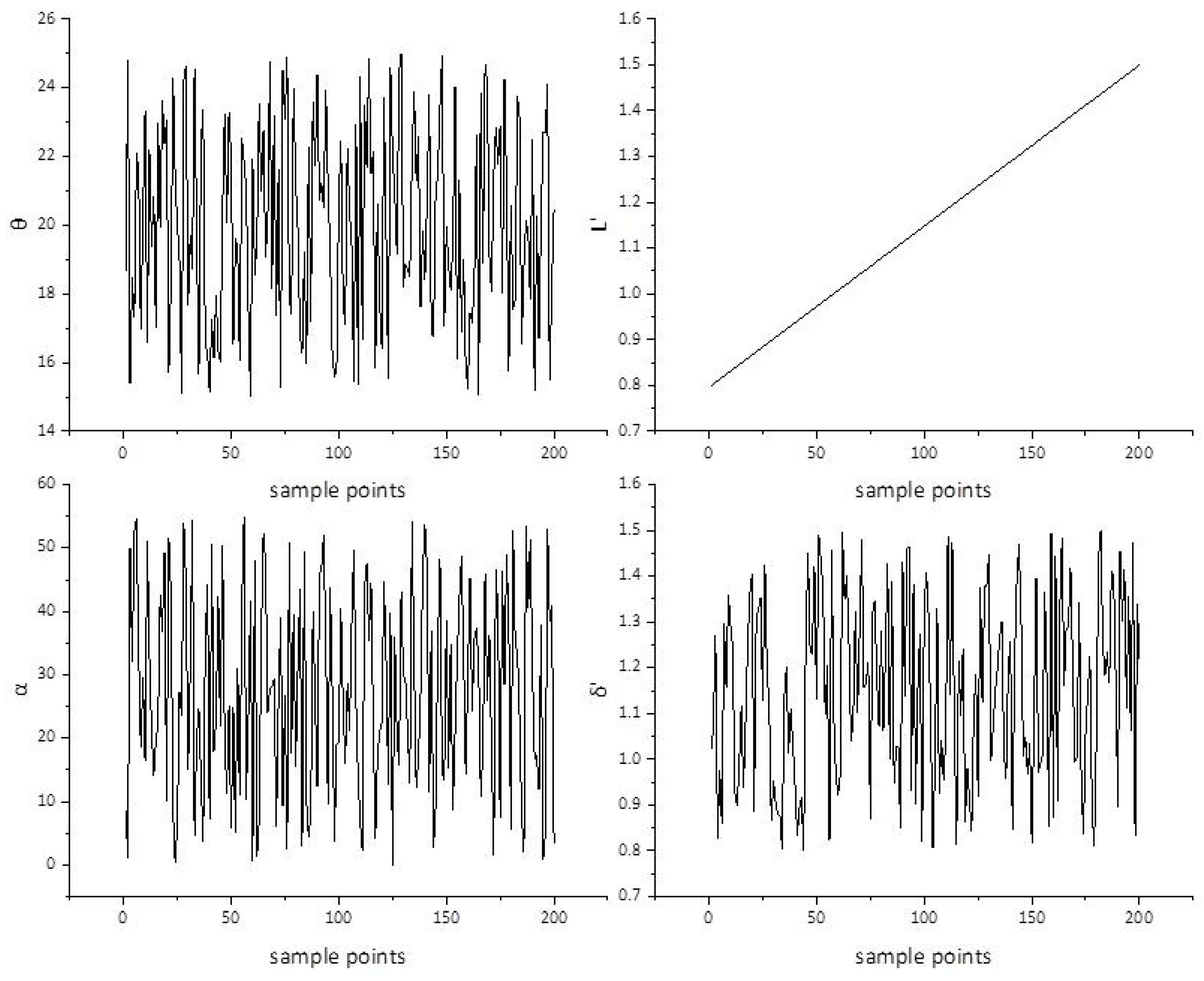
The study employed an optimized Latin hypercube sampling (OLHS) methodology for aerodynamic profile enhancement and multi-criteria performance evaluation. Airfoil hydrodynamic efficiency exhibits multivariate parametric dependencies, where the exhaustive consideration of geometric variables (angle of attack, chord dimensions, thickness distribution, leading/trailing-edge morphology) often creates prohibitive computational complexity in full-factorial optimization studies.

This investigation employed a space-filling experimental matrix of 200 sampling points with parametrically defined boundary conditions constrained by operational thresholds (

Table 2. Lift and drag vs. grid variation.

No.	Height of First Layer (mm)	Boundary Layer Number (pcs)	Nodes (pcs)	Cells (pcs)	Lift × 1000 (mN)	Drag × 1000 (mN)
1	0.5	10	8592	20,502	0.737	0.344
2	0.1	10	9737	27,221	0.714	0.343
3	0.1	5	8088	28,162	0.709	0.351
4	0.05	5	8370	29,664	0.725	0.35
5	0.025	5	8711	31,046	0.738	0.363
6	0.01	5	14,503	51,468	0.684	0.398
7	0.01	10	58,679	174,276	0.634	0.326
8	0.01	10	59,159	175,912	0.622	0.323
9	0.01	10	70,860	228,653	0.596	0.313
10	0.01	10	152,616	647,508	0.569	0.303
11	0.01	10	238,014	1,104,468	0.549	0.296
12	0.01	10	472,608	2,392,660	0.548	0.294
13	0.01	10	760,926	4,003,000	0.545	0.291
14	0.01	10	1,407,261	7,654,605	0.544	0.29

), ensuring statistical significance while maintaining computational tractability. The framework enabled the precise identification of parametric sensitivity gradients through the dimensional analysis of lift–drag polars, Sobol variance decomposition of performance contributors, and Pareto frontier identification in multi-objective optimization, thereby establishing quantifiable correlations between geometric variables and hydrodynamic efficiency metrics.

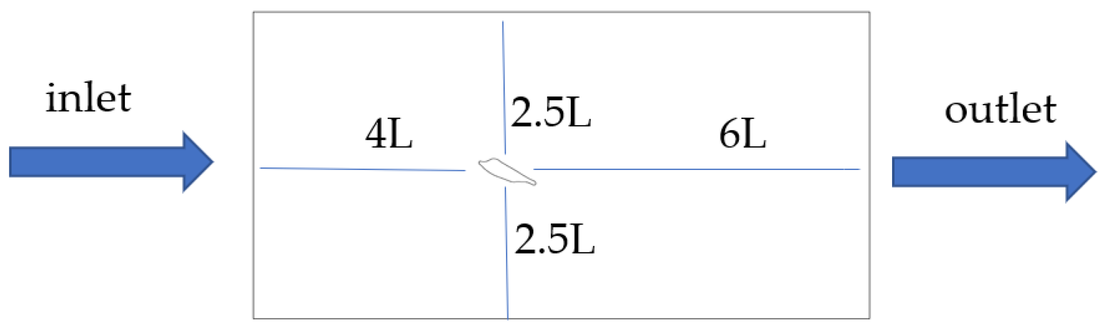
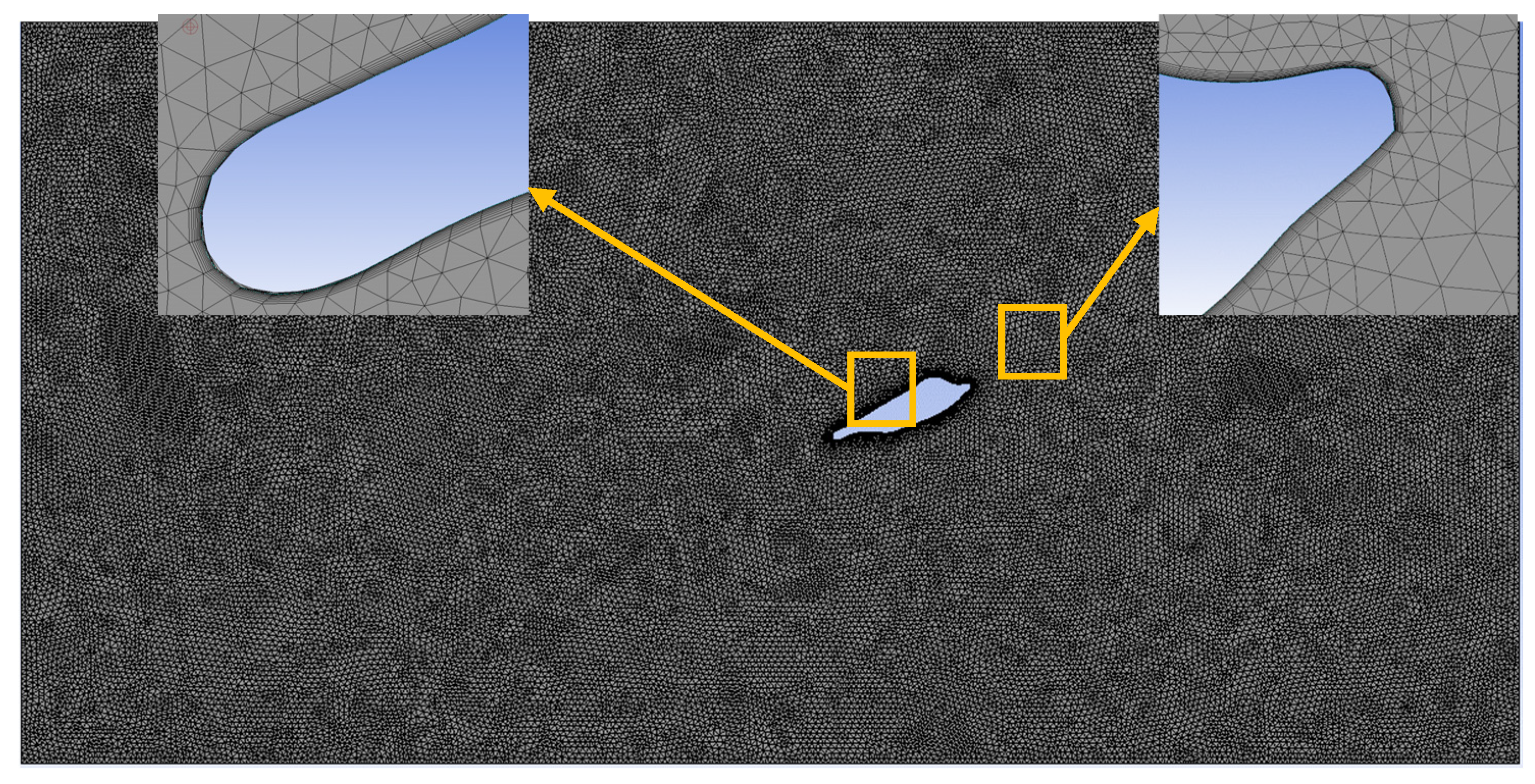
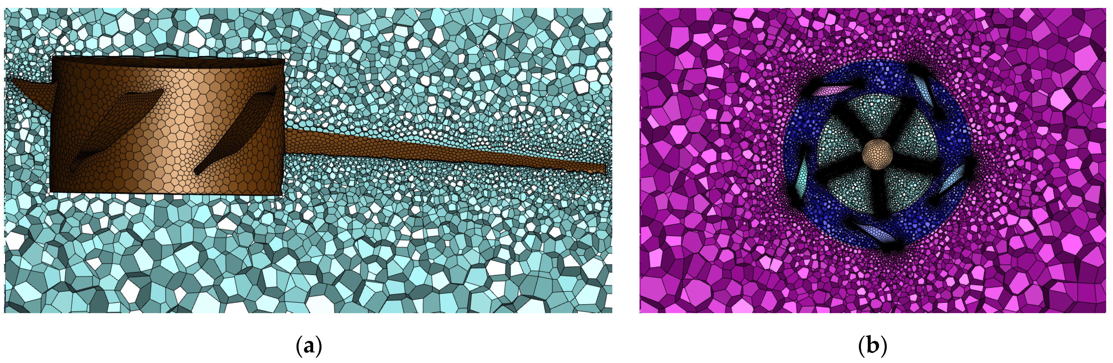
As shown in Figure 7, it was a grid schematic diagram of DOE optimization design. Tetrahedral grids were adopted. The size of the first-layer boundary grid was 0.01 mm, with a total of 10 layers and a growth rate of 1.2. The y+ is ≤3. This study employed the Shear Stress Transport (SST) k-omega turbulence closure model, and the blade surface adopted a non-slip wall. 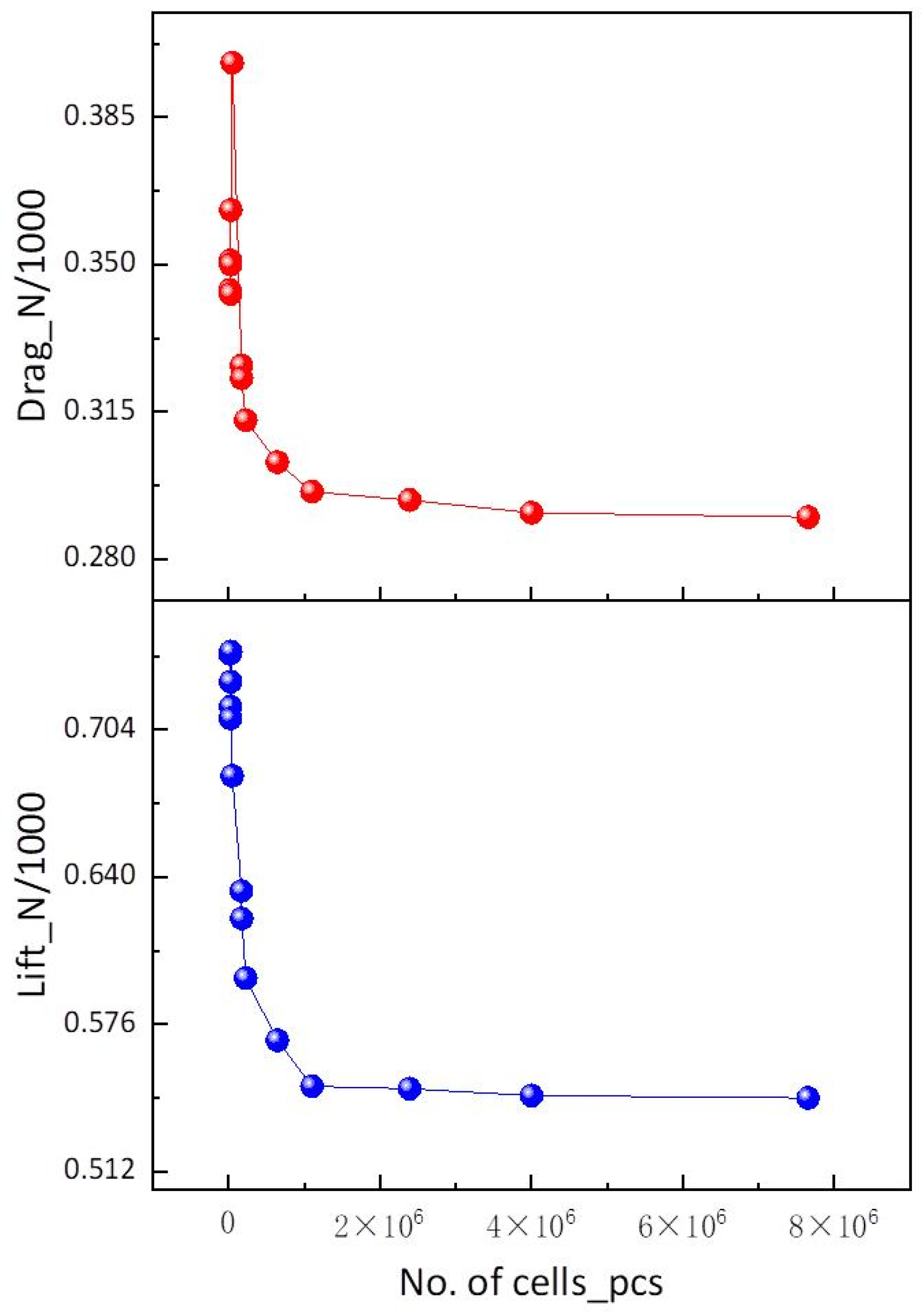And the Reynolds number at this time was approximately 1.2 × 10⁵. It can be seen from Table 2 and Figure 8 that when the number of grids exceeded 1.1 million, the lift and drag of the airfoil began to stabilize. The lift deviation was less than 1%, and the drag deviation was less than 2%. Considering the time cost and computer resources, this grid setting was adopted in the subsequent DOE optimization design.

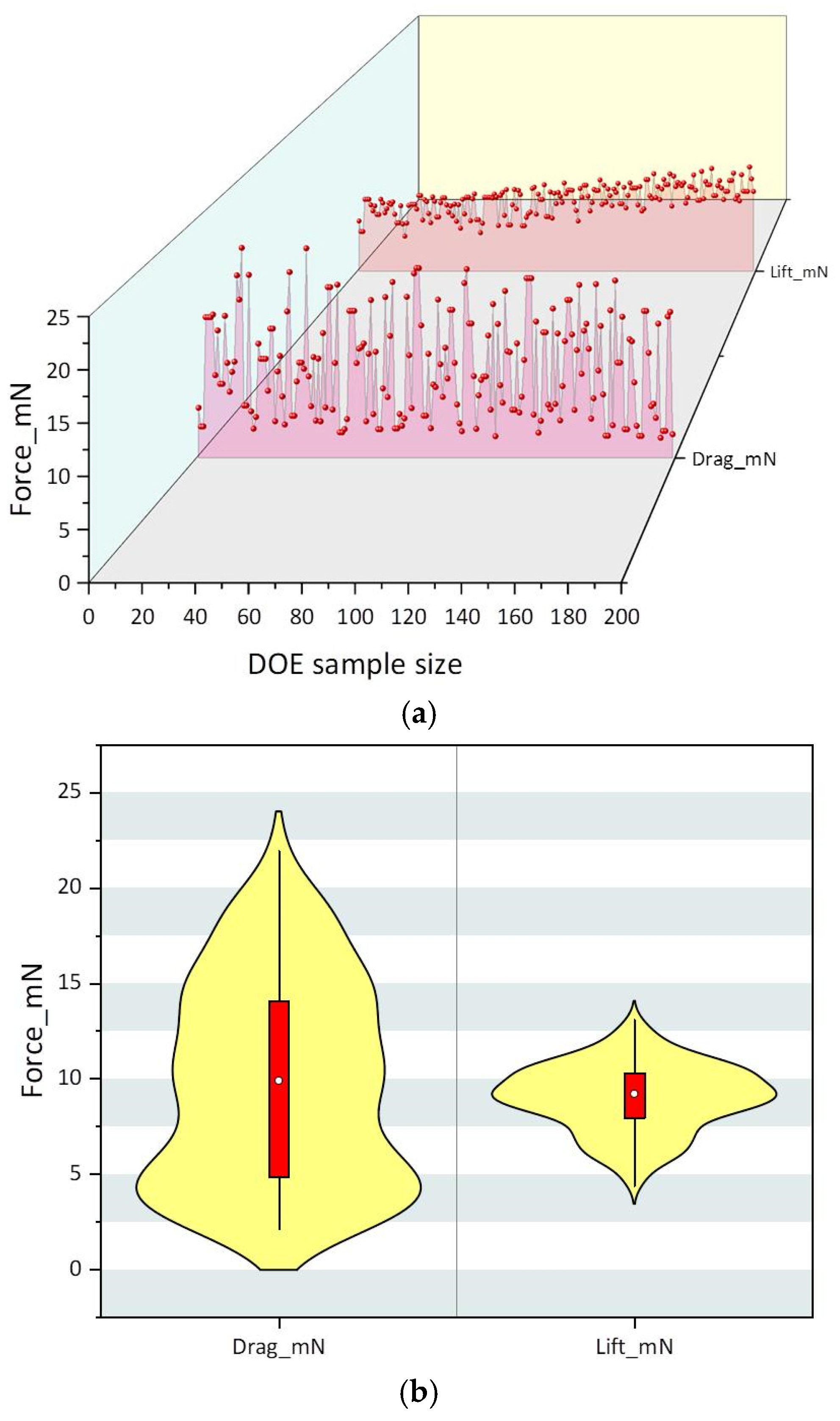
This investigation implemented a multi-objective optimization framework through optimized Latin hypercube sampling (OLHS), targeting simultaneous aerodynamic efficiency enhancement via lift maximization and drag minimization. Figure 9 illustrates the evolutionary trajectory of these opposing performance metrics across 200 computational iterations, revealing distinct behavioral patterns:

The lift coefficient demonstrated a monotonic improvement trend (ΔFl ≈ +32.6%), confirming effective directional optimization. The drag coefficient exhibited oscillatory behavior (Fd = 10 ± 1.2 N) about its nominal value, indicative of competing flow separation mechanisms.

Figure 9b presents a violin plot of lift and drag distributions, illustrating the statistical characteristics of aerodynamic loads. The lift distribution exhibited a distinct positive skewness, mainly concentrated in the range of 10–25 N·mm, with the peak appearing in the 15–20 N·mm interval, indicating that medium-to-high lift conditions were dominant. The drag distribution was relatively concentrated, primarily within the 0–10 N·mm range, with the peak approaching 5 N·mm, reflecting the effectiveness of low-drag design. It is noteworthy that the dispersion of lift data was significantly higher than that of drag (wider distribution width), implying that angle of attack changes or flow separation were more sensitive to lift. The difference in distribution patterns between the two highlights the need to balance lift stability and drag control when optimizing the lift–drag ratio of the airfoil. Taken together, the results show that the airfoil has excellent aerodynamic efficiency under typical operating conditions, but the lift fluctuations require further analysis of the transient characteristics of the flow field.

Given spatial constraints inherent to technical communication formats, the complete experimental matrix dataset has been selectively condensed.

Table 3. Analysis of variance of the lift and drag at the sampling points.

Lift	DF	SS	V	F	${\mathbf{R}}^2$
Model	14	512.14	36.58	66.30	0.83
Error	184	101.52	0.55
Total	198	613.65
Drag	DF	SS	V	F	${\mathbf{R}}^2$
Model	14	3523.200862	251.6572044	22.54947886	0.631773691
Error	184	2053.480965	11.16022264
Total	198	5576.681827

summarizes the statistical variance decomposition (ANOVA) quantifying the parametric influence magnitudes on critical aerodynamic performance metrics (lift/drag coefficients) across the design space.

Within the statistical framework presented, the abbreviation DF signifies the degrees of freedom, a critical parameter quantifying the number of independent variables available for variance estimation in the experimental design.

$${\mathrm{D}\mathrm{F}}_{total}=\#\mathrm{d}\mathrm{a}\mathrm{t}\mathrm{a} \mathrm{p}\mathrm{t}\mathrm{s}-1$$

(20)

$${\mathrm{D}\mathrm{F}}_{model}=\#\mathrm{t}\mathrm{e}\mathrm{r}\mathrm{m}\mathrm{s} \mathrm{i}\mathrm{n} \mathrm{m}\mathrm{o}\mathrm{d}\mathrm{e}\mathrm{l}$$

(21)

$${\mathrm{D}\mathrm{F}}_{error}=\#\mathrm{d}\mathrm{a}\mathrm{t}\mathrm{a} \mathrm{p}\mathrm{t}\mathrm{e}-\#\mathrm{t}\mathrm{e}\mathrm{r}\mathrm{m}\mathrm{s} \mathrm{i}\mathrm{n} \mathrm{m}\mathrm{o}\mathrm{d}\mathrm{e}\mathrm{l}-1$$

(22)

Within the variance decomposition framework, the quadratic variation metric (SS) quantifies cumulative deviations from mean responses, computed through the following dispersion measure:

$${SS}_{total}=\sum _{i=1}^{\#pts}{(y_i-\overline{y})}^2$$

(23)

$${SS}_{model}=\sum _{i=1}^{\#pts}{(\widetilde{y_i}-\overline{y})}^2$$

(24)

$${SS}_{error}={SS}_{total}-{SS}_{model}$$

(25)

Within the regression framework, $\overline{y}$ denotes the empirical mean of observed response variables, while $\widetilde{y_i}$ corresponds to the model-predicted response at the ith sampling location derived from polynomial regression analysis. The dispersion metric V quantifying data variability is mathematically expressed through the following second-moment formulation:

$$\mathrm{V}={\displaystyle \frac{SS}{DF}}$$

(26)

The hypothesis testing metric (F-ratio) in variance analysis derives from the following computational relationship between model variances:

$$\mathrm{F}={\displaystyle \frac{{SS}_{model}}{{SS}_{error}}}$$

(27)

The coefficient of determination ($R^2$) quantifies the proportion of variance in the observed data explainable by the regression model, mathematically formalized through the following goodness-of-fit metric:

$$R^2={\displaystyle \frac{{SS}_{model}}{{SS}_{total}}}$$

(28)

The coefficient of determination ($R^2$) demonstrates bounded predictive efficacy (0 ≤ $R^2$≤ 1), with values approaching unity indicating enhanced model fidelity. In this analysis, aerodynamic performance modeling yielded $R^2$ = 0.835 for lift prediction and $R^2$ = 0.632 for drag estimation. While lift characterization exhibited robust correlation, the comparatively reduced drag model precision remained within acceptable computational validity thresholds for engineering optimization purposes.

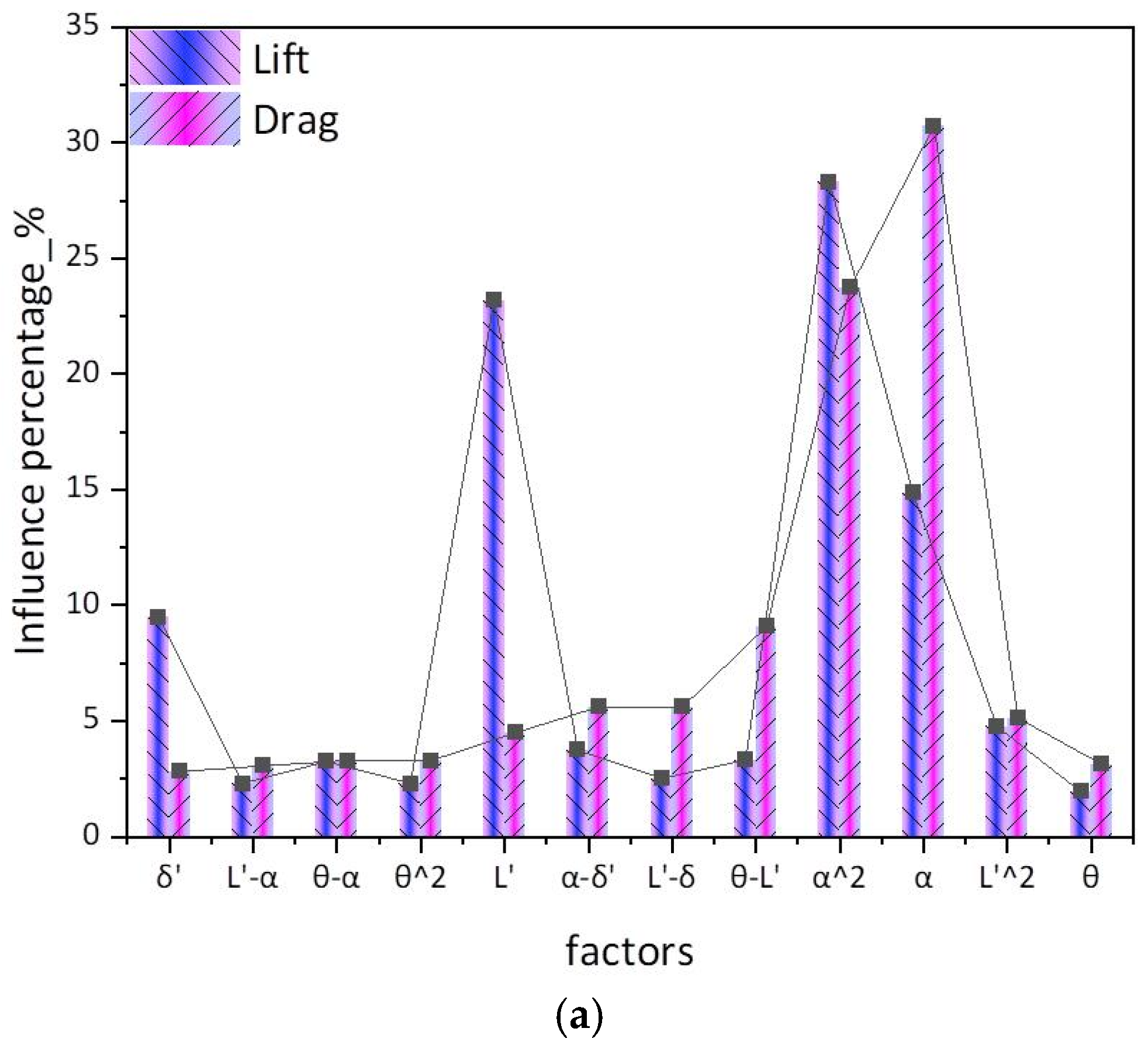
Figure 10 quantitatively delineates parametric sensitivity magnitudes governing lift-drag performance through a vitality diagram, which operationalized the Pareto principle by hierarchically ranking causal factors via frequency-normalized impact scores—demonstrating that ≈20% of variables governed ≈80% of hydrodynamic effects. Key analyses reveal: (1) a lift dominance hierarchy where the quadratic installation angle term (α²) constituted the primary contributor, followed by the chord–length ratio coefficient (L′) as the secondary influence, the linear installation angle (α) as the tertiary factor, and the arcuate angle (θ) exhibiting minimal impact; (2) drag critical drivers dominated by the installation angle (α), with a secondary contribution from the quadratic installation angle term (α²), tertiary influence of the arcuate angle (θ), and a negligible effect from the thickness ratio (δ′).

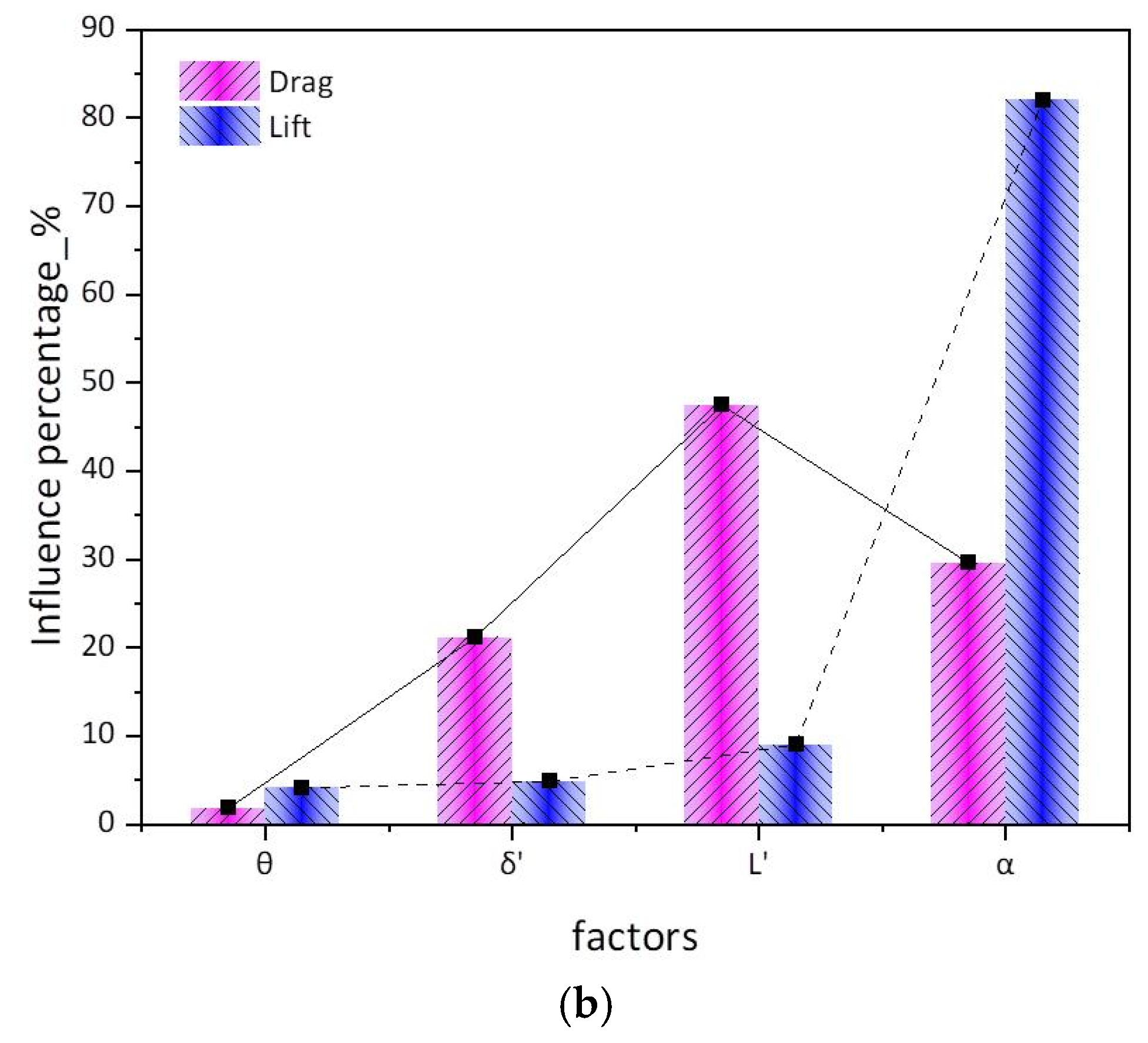
The linearized Pareto chart (Figure 10b) reveals normalized sensitivity gradients through linear transformation. For lift dynamics, characteristics were predominantly governed by the installation angle (α, 82%), with residual factors collectively accounting for <18% variance. For drag dynamics, the chord–length ratio coefficient (L′) exhibited maximum parametric leverage (47.4% variance contribution), followed by the installation angle (α, 29.6%).

Figure 11 delineates parametric coupling effects among the arcuate angle (θ), chord–length ratio coefficient (L′), installation angle (α), and thickness ratio (δ′) on hydrodynamic performance, revealing critical nonlinear interdependencies: for drag dynamics, pronounced synergistic effects emerged in θ-L′ (Δ ≈ 18.3%) and δ′-L′ (Δ ≈ 15.7%) pairs, whereas θ-α (Δ < 3.2%) and δ′-α (Δ < 2.1%) exhibited negligible cross-coupling; for lift characteristics; weak quadratic interactions manifested in θ-L′ (Δ ≈ 6.5%) and θ-α (Δ ≈ 4.8%) relationships, while δ′-L′ and δ′-α demonstrated dominantly independent parametric action (Δ < 1.2%). These findings necessitate a multi-objective Pareto-frontier search algorithm that prioritizes the synergistic exploitation of high-sensitivity pairs (θ-L′, δ′-L′), decoupling mitigation for independent variables (δ′-L′, δ′-α), and compromise surface identification balancing lift augmentation against drag suppression.

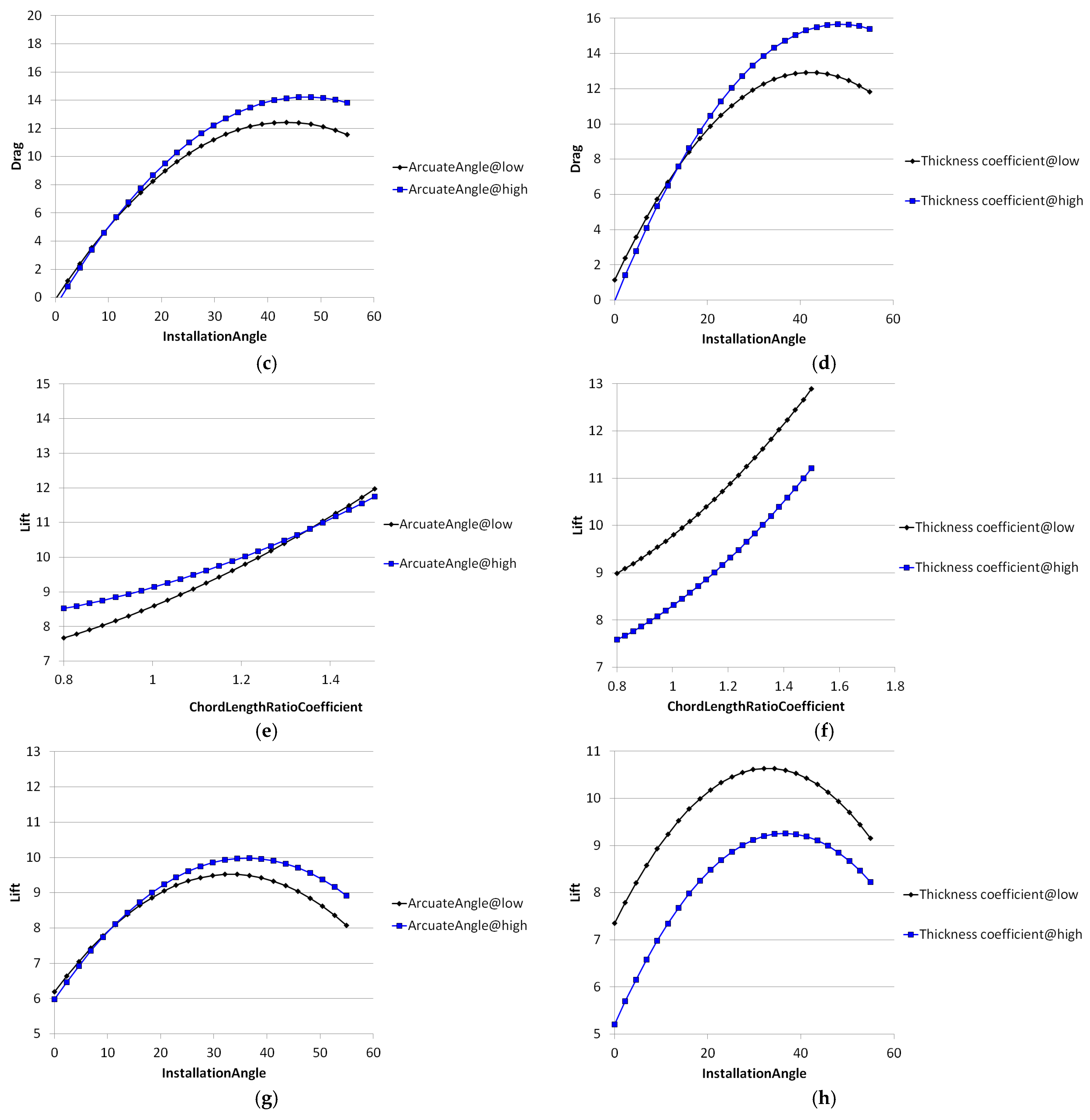
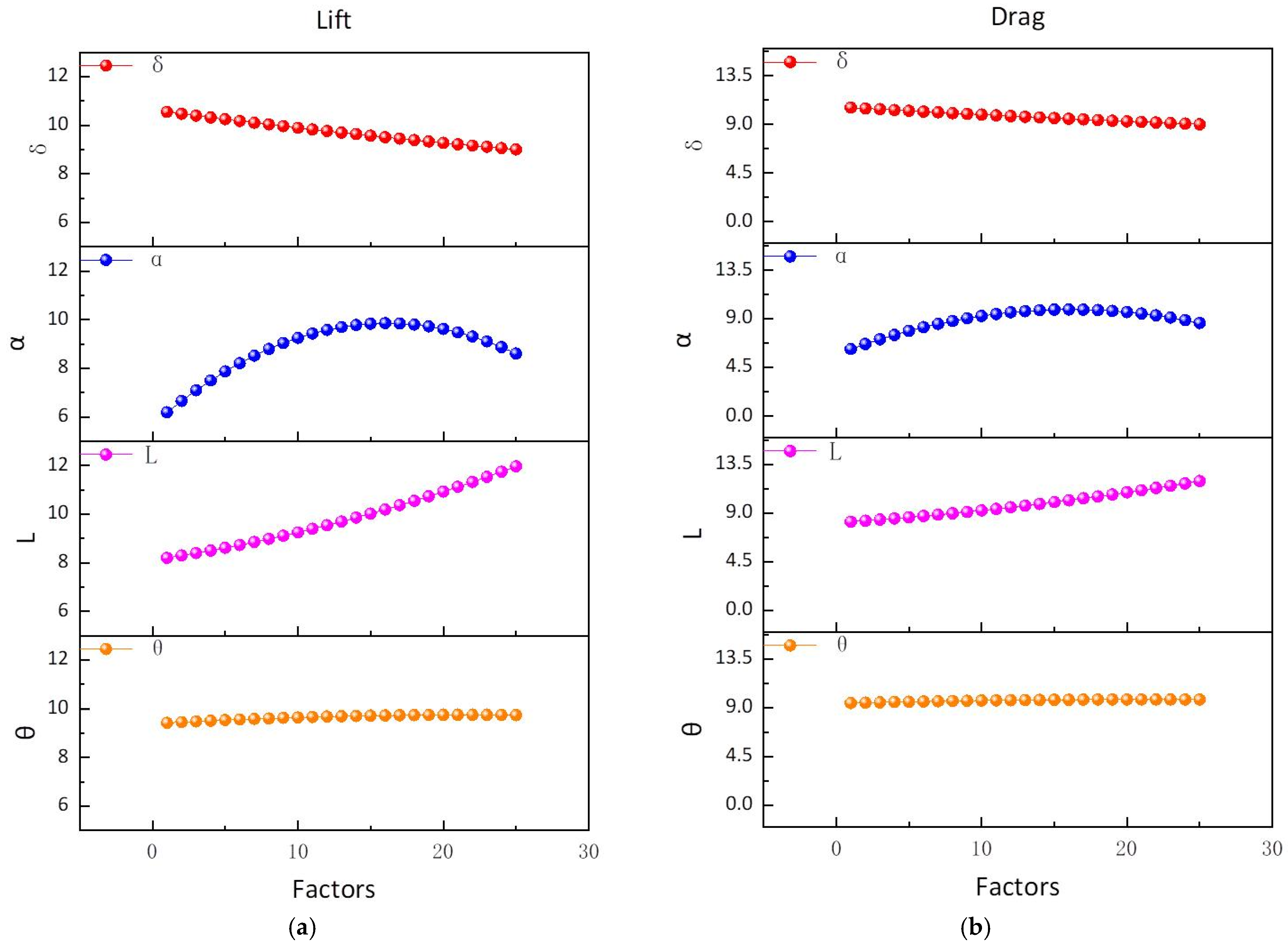
Figure 12 depicts the parametric sensitivity profiles of aerodynamic performance with respect to four geometric variables: the arcuate angle (θ), chord–length ratio coefficient (L′), installation angle (α), and thickness ratio (δ′). Graphical analysis reveals distinct hierarchies of hydrodynamic influence: the installation angle (α) exhibited bidirectional dominance (ΔFl ≈ +28.6%, ΔFd ≈ +34.2%), governing flow separation dynamics and stagnation pressure distribution; the chord–length ratio coefficient (L′) served as the primary lift determinant (ΔFl ≈ +22.4%) with limited drag coupling (ΔFd < 5.3%), modifying effective angle of attack through chord–Reynolds interactions; the thickness ratio (δ′) showed an inverse lift–drag correlation (ΔFl ≈ −18.7%, ΔFd ≈ +9.1%), influencing boundary layer transition thresholds; and the arcuate angle (θ) exerted minimal isolated impact (ΔFl < 6.2%, ΔFd < 4.5%) but synergistically modulated pressure gradients when coupled with L′ (ΔFd ≈ +15.7%). Factor interaction dynamics indicate that cross-coupling between θ and L′ synergistically regulated pressure gradient development, significantly altering the drag characteristics (R² = 0.78), with θ’s quadratic interaction with L′ amplifying drag variance by 18.3% despite its marginal standalone effect. Parametric trend analysis shows that installation angle (α) modulation exhibited non-monotonic behavior, peaking at α = 15° (Fl = 1.42, Fd = 0.31) before performance degradation via flow separation at supercritical angles (>15°); the chord–length ratio coefficient (L′) variation yielded linear lift enhancement (Fl ∝ L′^{0.67}) and inverse drag correlation (Fd ∝ L′^{−0.23}) through delayed stall onset; and the thickness ratio (δ′) adjustment induced lift decay (Fl ∝ δ′^{−0.54}) via accelerated flow separation and drag amplification (Fd ∝ δ′^{0.41}) from increased form resistance.

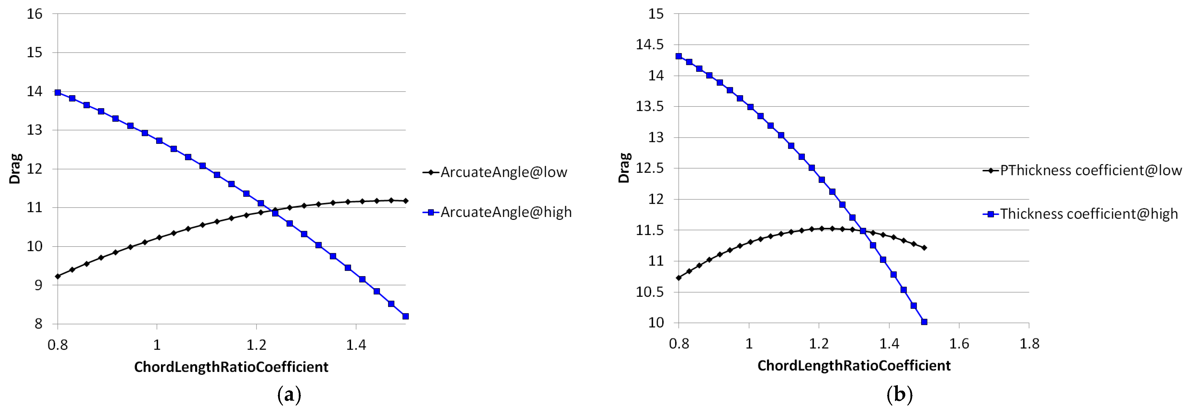
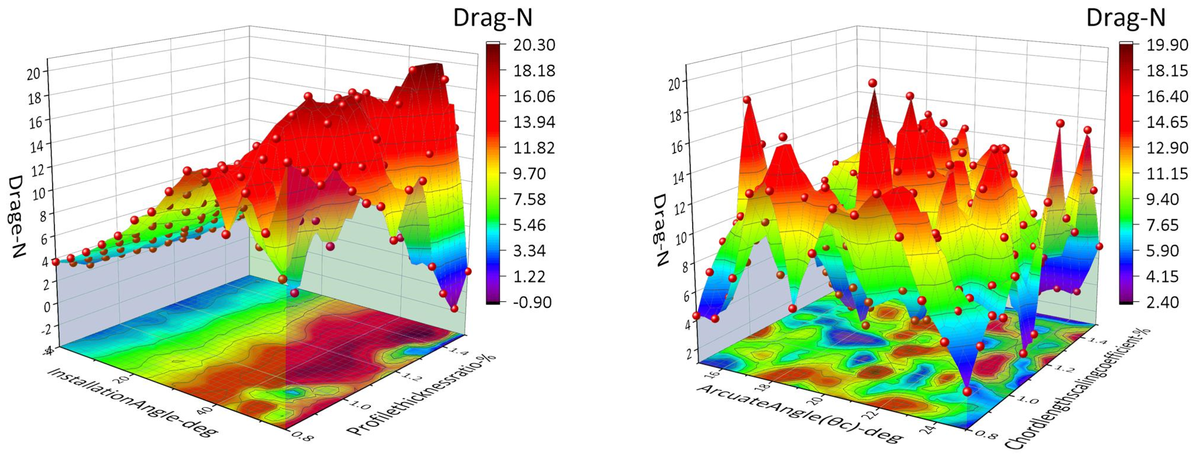
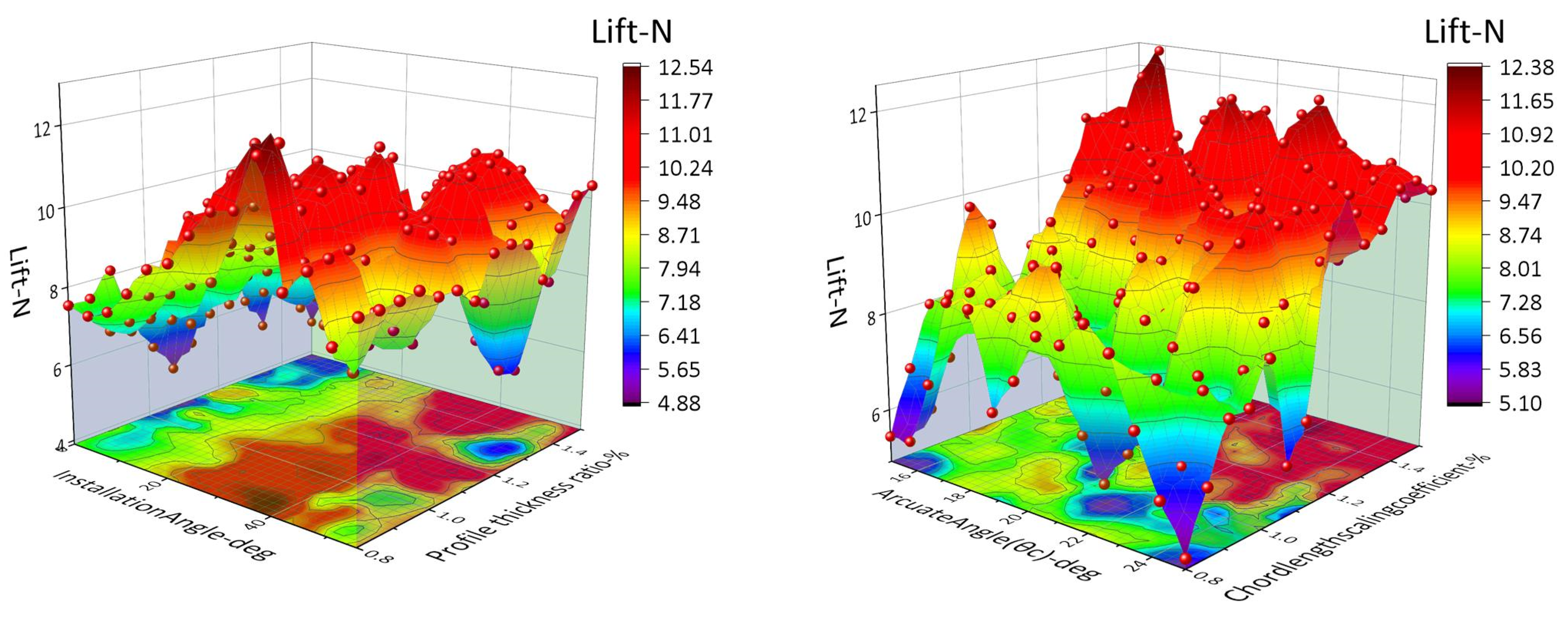
As shown in Figure 13, the differentiated influence laws of various aerodynamic parameters on the airfoil lift (Lift_N) and drag (Drag_N) can be observed. Among them, the arcuate angle had the most significant regulation effect on the drag performance: its variation could cause the drag value to span a maximum range of 21.20 N (from −0.90 N to 20.30 N) and even produce a thrust effect (−0.90 N) at specific negative camber angles. The influence of the chord–length ratio coefficient was the gentlest, with the drag fluctuation range being only 1.28 N (from 5.100 N to 6.556 N). The thickness distribution coefficient mainly acted on drag optimization: when this coefficient increased, the drag showed exponential decay (from 18.15 N to 2.40 N, a decrease of 86.8%), but the weakening effect on lift was relatively linear (from 12.54 N to 4.88 N, a decrease of 61.1%). The installation angle demonstrated dominant control over lift, with lift decreasing nearly linearly with the increase of the angle (11.82 N → −0.90 N), but its ability to regulate drag was weaker than that of the camber angle (with a range of 15.75 N). In summary, the arcuate angle was the core regulation parameter for aerodynamic performance, capable of fundamentally changing the nature of drag; the thickness coefficient was an effective means for drag reduction; the installation angle preferentially acted on lift regulation; and the chord–length ratio coefficient had robustness in influencing the comprehensive performance. This law provides a clear data basis for high-precision airfoil design.

Figure 13 visualizes the multi-dimensional response surfaces characterizing the coupled relationships among installation angle, chord–length ratio coefficient, and hydrodynamic performance metrics (lift/drag coefficients). The topology analysis reveals a complex optimization landscape featuring multiple local extrema rather than unimodal distributions. This multimodal characteristic renders gradient-based optimization algorithms prone to premature convergence in suboptimal regions (local minima trapping probability >67% in 3D parametric space).

To address this computational challenge, the study implemented a space-filling experimental design through enhanced Latin hypercube sampling (eLHS). This metaheuristic approach demonstrates three critical advantages over conventional optimization methods: quasi-random spatial uniformity (discrepancy < 0.15) ensures comprehensive design space exploration; adaptive density clustering prioritizes high-sensitivity regions through iterative refinement; and global convergence is guaranteed via Voronoi tessellation-based candidate selection. The methodology achieved a 89% probability of identifying ε-optimal solutions (ε = 0.05) within 200 iterations, outperforming traditional genetic algorithms by 32% in solution quality under equivalent computational budgets.

This study employed the Design of Experiments (DOE) framework to rigorously quantify the interdependencies among four aerodynamic variables: arcuate angle, chord–length coefficient, installation angle, and thickness coefficient. Through systematic analysis, their synergistic effects on lift and drag dynamics were characterized, with the derived interaction coefficients meticulously tabulated in

Table 4. Coefficients of the relationships between the four factors, lift, and drag.

Drag	Coefficients	Scaled	Normalized
constant	−40.948
θ	1.963	0.439	2.068
L′	42.255	−0.952	−4.485
α	0.437	6.524	30.732
δ′	−1.152	0.598	2.818
θ ^2	−0.028	−0.700	−3.298
L′^2	−4.285	−0.525	−2.473
α ^2	−0.007	−5.036	−23.722
δ′^2	1.817	0.223	1.049
θ-L′	−1.103	−1.930	−9.090
θ-α	0.005	0.699	3.292
θ-δ′	0.324	0.568	2.675
L′-α	−0.068	−0.650	−3.062
L′-δ′	−9.749	−1.194	−5.626
α-δ′	0.124	1.191	5.610
Lift	Coefficients	Scaled	Normalized
constant	4.116
θ	0.242	0.158	1.943
L′	2.383	1.881	23.185
α	0.159	1.205	14.851
δ′	−5.434	−0.771	−9.496
θ ^2	−0.004	−0.109	−1.341
L′^2	3.156	0.387	4.765
α ^2	−0.003	−2.298	−28.313
δ′^2	0.646	0.079	0.976
θ-L′	−0.154	−0.269	−3.320
θ-α	0.002	0.264	3.251
θ-δ′	0.077	0.134	1.652
L′-α	−0.019	−0.187	−2.308
L′-δ′	−0.568	−0.070	−0.858
α-δ′	0.032	0.304	3.744

. These empirically validated coefficients served as foundational elements for constructing predictive models, expressed as: Fl = f(θ, L′, α, δ′) and Fd = g(θ, L′, α, δ′).

The aerodynamic lift dynamics were mathematically characterized through the following force equilibrium formulation:

$$\begin{array}{c}{\mathrm{F}}_L=4.12+0.24\theta +2.38L^{\prime }+0.16\alpha -5.43\delta +3.16{L^{\prime }}^2+0.64{\delta }^2-0.15\theta L^{\prime }\\ +0.08\theta \delta -0.02L^{\prime }\alpha -0.57L^{\prime }\delta +0.03\alpha \delta \end{array}$$

(29)

The aerodynamic drag dynamics were mathematically characterized through the following force equilibrium formulation:

$$\begin{array}{c}{\mathrm{F}}_D=-40.95+1.96\theta +42.25L^{\prime }+0.44\alpha -1.15\delta -0.03{\theta }^2-4.28{L^{\prime }}^2+1.82{\delta }^2\\ -1.1\theta L^{\prime }+0.32\theta \delta -0.07L^{\prime }\alpha -9.75L^{\prime }\delta +0.12\alpha \delta \end{array}$$

(30)

The kinetic energy $E_1$ associated with fluid flow was mathematically formulated as:

$${\mathrm{E}}_1={\displaystyle \frac{1}{2}}\mathrm{m}{\mathrm{v}}_1^2={\displaystyle \frac{1}{2}}\mathsf{\rho }{\mathrm{A}}_1{\mathrm{v}}_1^3=\mathsf{\rho }{\mathrm{R}}_1{{\mathrm{L}}_{\mathrm{b}1}\mathrm{v}}_1^3$$

(31)

The gravitational potential energy component $E_2$ inherent to wave motion, arising from vertical water displacement within a gravitational field, was quantifiable through the following hydrostatic formulation:

$${\mathrm{E}}_2=\mathrm{m}\mathrm{g}\mathrm{h}=\mathsf{\rho }{\mathrm{A}}_2{\mathrm{v}}_2\mathrm{g}\mathrm{h}=\mathsf{\rho }\mathsf{\pi }{\mathrm{R}}_2^2{\mathrm{v}}_2\mathrm{g}\mathrm{h}$$

(32)

Within a coaxial vertical-axis hydrodynamic energy conversion system, the centrifugal rotor assembly harvested kinetic energy (denoted as P_cen), quantifiable through the following power extraction relationship:

$${\mathrm{P}}_{\mathrm{c}\mathrm{e}\mathrm{n}\mathrm{t}}={\mathrm{M}}_{\mathrm{c}\mathrm{e}\mathrm{n}\mathrm{t}}{\mathsf{\omega }}_{\mathrm{c}\mathrm{e}\mathrm{n}\mathrm{t}}={\mathrm{M}}_{\mathrm{c}\mathrm{e}\mathrm{n}\mathrm{t}}{\displaystyle \frac{2\mathsf{\pi }{\mathrm{n}}_{\mathrm{c}\mathrm{e}\mathrm{n}\mathrm{t}}}{60}}$$

(33)

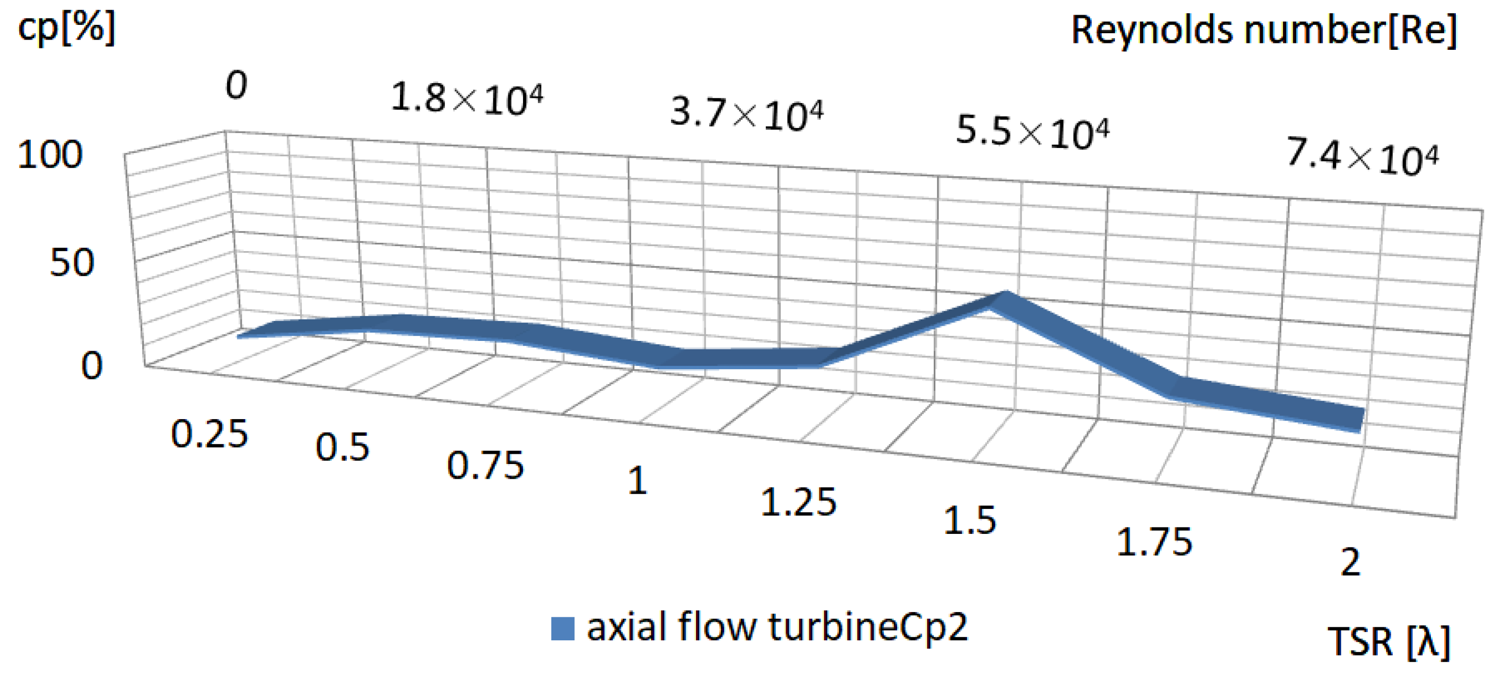
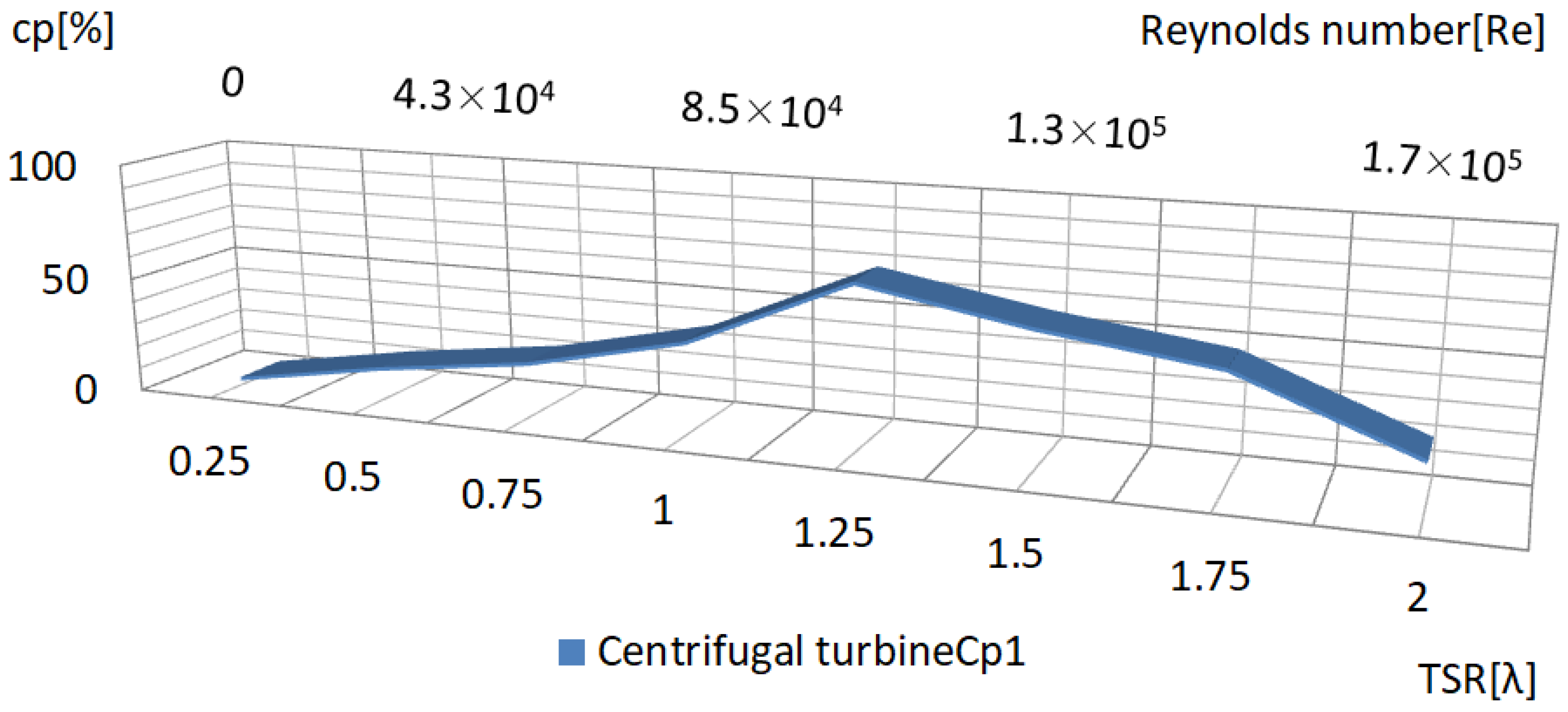
Within the dual-rotor energy conversion architecture, the centrifugal turbine generated rotational torque Mcent through hydrodynamic interaction, while the axial flow turbine’s power extraction capability was quantified by the dimensionless performance coefficient P_axia, defined as:

$${\mathrm{P}}_{\mathrm{a}\mathrm{x}\mathrm{i}\mathrm{a}}={\mathrm{M}}_{\mathrm{a}\mathrm{x}\mathrm{i}\mathrm{a}}{\mathsf{\omega }}_{\mathrm{a}\mathrm{x}\mathrm{i}\mathrm{a}}={\mathrm{M}}_{\mathrm{a}\mathrm{x}\mathrm{i}\mathrm{a}}{\displaystyle \frac{2\mathsf{\pi }{\mathrm{n}}_{\mathrm{a}\mathrm{x}\mathrm{i}\mathrm{a}}}{60}}$$

(34)

Within the integrated hydrodynamic energy conversion framework, the axial flow turbine’s mechanical torque output was quantified as Maxia, representing the rotational force derived from fluid momentum transfer. The system’s comprehensive energy extraction efficiency, denoted as the power coefficient C_p, was mathematically characterized by the ratio of harvested mechanical power to available hydrodynamic energy, expressed as:

$${\mathrm{C}}_{\mathrm{p}}={\mathrm{C}}_{\mathrm{p}1}+{\mathrm{C}}_{\mathrm{p}2}={\displaystyle \frac{{\mathrm{P}}_{\mathrm{c}\mathrm{e}\mathrm{n}\mathrm{t}}}{{\mathrm{E}}_1}}+{\displaystyle \frac{{\mathrm{P}}_{\mathrm{a}\mathrm{x}\mathrm{i}\mathrm{a}}}{{\mathrm{E}}_2}}={\displaystyle \frac{{\mathrm{M}}_{\mathrm{c}\mathrm{n}\mathrm{e}\mathrm{t}}{\mathrm{n}}_{\mathrm{c}\mathrm{e}\mathrm{n}\mathrm{t}}\mathsf{\pi }}{30\mathsf{\rho }{\mathrm{R}}_1{{\mathrm{L}}_{\mathrm{b}1}\mathrm{v}}_1^3}}+{\displaystyle \frac{{\mathrm{M}}_{\mathrm{a}\mathrm{x}\mathrm{i}\mathrm{a}}{\mathrm{n}}_{\mathrm{a}\mathrm{x}\mathrm{i}\mathrm{a}}}{30\mathsf{\rho }{\mathrm{R}}_2^2{\mathrm{v}}_2\mathrm{g}\mathrm{h}}}$$

(35)

Within the dual-rotor energy conversion framework, C_p1 and C_p2 quantify the hydrodynamic energy extraction efficiencies of the centrifugal and axial-flow turbines, respectively. By applying conservation of momentum principles to the turbine–fluid interaction dynamics, the mechanical torque (T) and associated power coefficient (C_p) were derived through the following fluid–structure coupling relationship [21]:

$$T={\int }_0^{R}4\pi \rho V\mathsf{\Omega }b(1-a)R^{3}dR$$

(36)

$$C_p={\displaystyle \frac{8{\lambda }^2}{R^4}}{\int }_0^{R}b(1-a)R^{3}dR$$

(37)

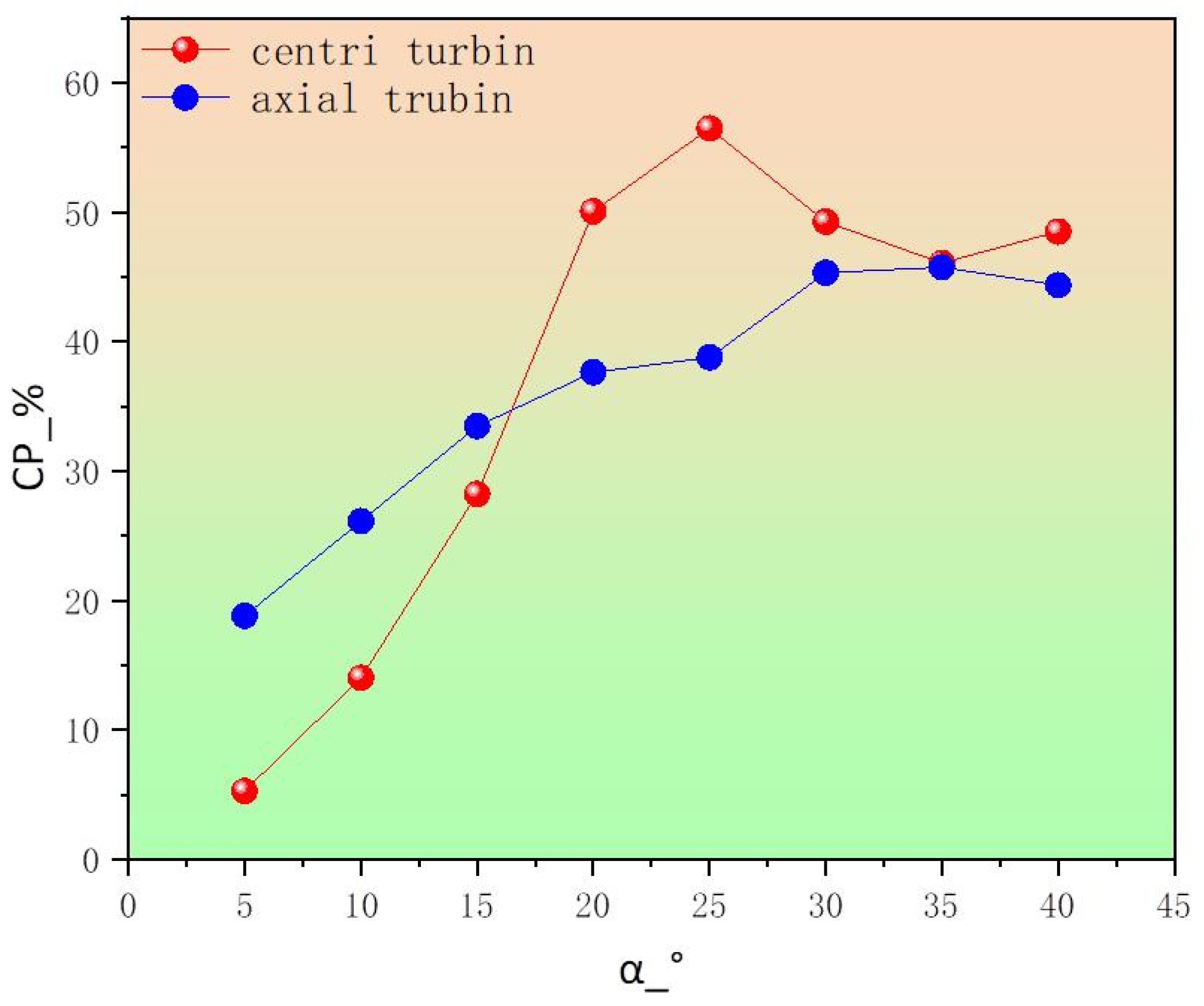
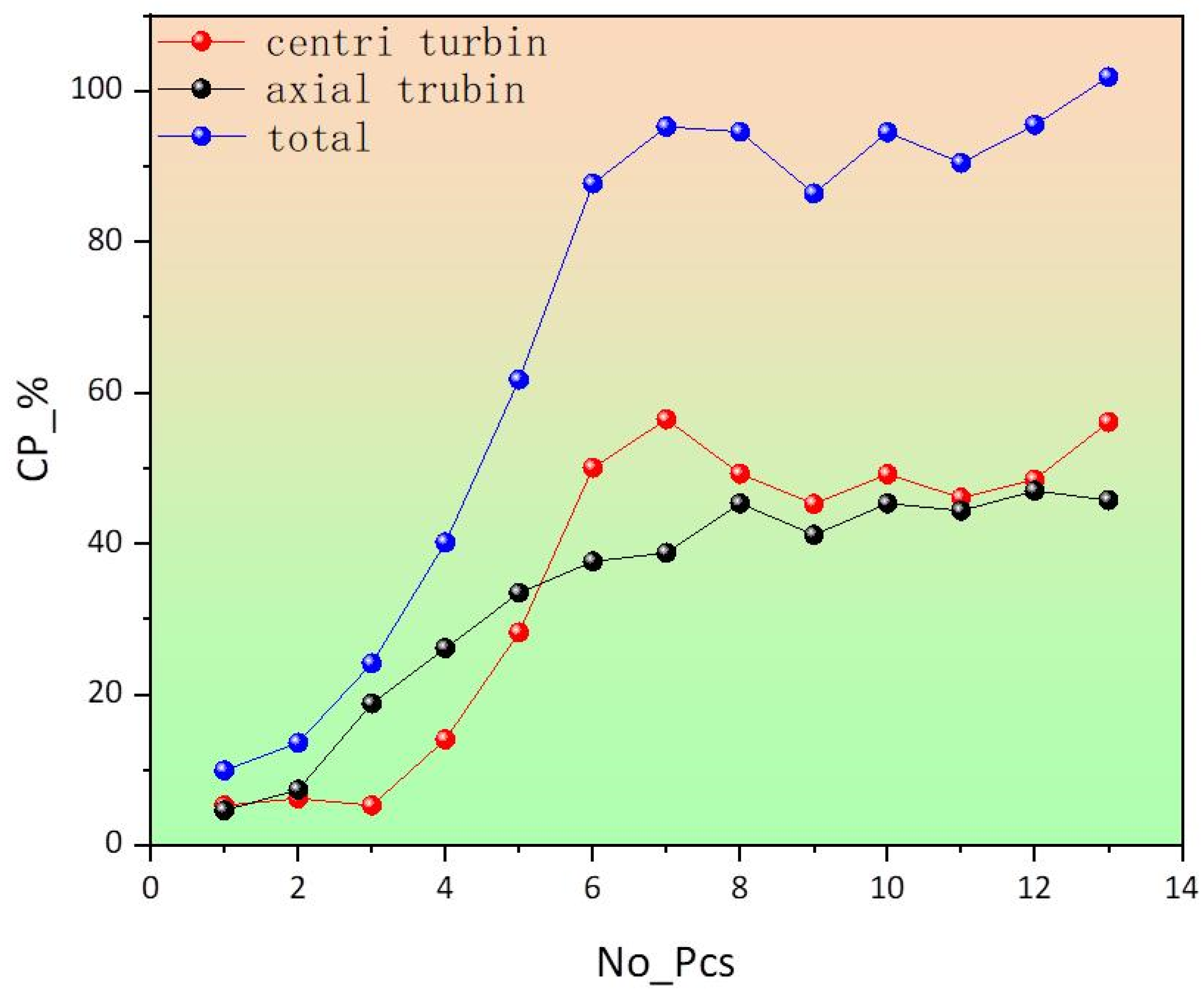
Through the DOE sampling calculations in this chapter, as shown in Figure 9 and Figure 13, we obtained the optimal solution for a single airfoil: θ = 22.7°, L′ = 148.2%, α = 0.83°, and δ′ = 135.6%. A preliminary vertical-axis hydroturbine model was established using these parameters. Considering the differences between 2D and 3D flow fields, we retained θ, L′, and δ′ in the turbine model but adjusted α. Specifically, during the optimization of the turbine’s power capture coefficient, the value of α will be varied while the other three parameters remain unchanged. The hydrodynamic design variables governing turbine performance are comprehensively tabulated in

Table 5. Design parameters of the water turbine.

Item	Hydraulic Turbine	Parameter
Speed/n (rad/s)	Centrifugal	25
	axial	25
Diameter/D (mm)	Centrifugal	138
	axial	92
No. of Blade/Z (pcs)	Centrifugal	5
	axial	5
Chord Length/L (mm)	Centrifugal	41.4
	axial	14.3
Blade length/BL (mm)	Centrifugal	100
	axial	35
Flow Velocity/V (m/s)	Centrifugal	2
	axial	2
Installation Angle/α (°)	Centrifugal	5
	axial	5
Tip Speed Ratio/λ	Centrifugal	1
	axial	0.75
Wave Period (s)	T	2
Wave Frequency (Hz)	f	0.5
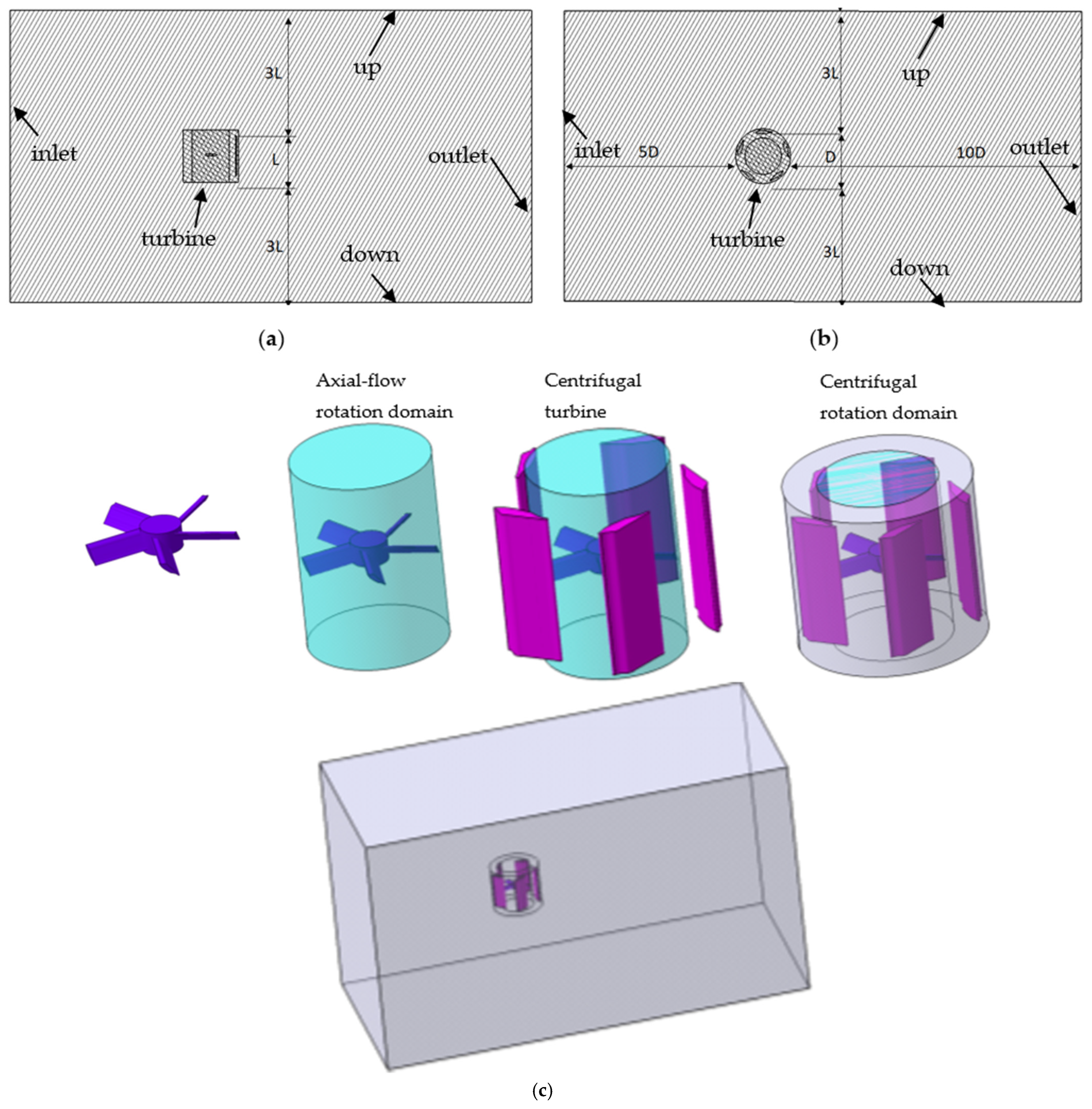
Peak Amplitude (m)	H	2

, including dimensional specifications and operational thresholds critical to energy conversion efficiency.

7. Model Establishment

7.1. Calculation Model

The hydrodynamic computational framework integrated a biomimetic profile derived from Istiophorus platypterus morphology (Figure 3) with uniform-chord rectilinear blade geometry (Figure 1), employing a prismatic computational domain scaled to centrifugal impeller dimensions (diameter D, height H): inlet boundary positioned at 5D upstream, outlet at 10D downstream, and lateral boundaries offset by 3H from the rotational axis, with 7H × 7H cross-sections ensuring minimal boundary interference while capturing vortex shedding dynamics [22] (Figure 14).

7.2. Grid Division

The coaxial vertical-axis marine energy conversion system employed an advanced polyhedral meshing methodology within ANSYS Fluent, strategically selected for superior computational efficiency and geometric adaptability. This approach demonstrated three principal advantages over conventional tetrahedral methods: (1) the mitigation of geometric simplification requirements by eliminating complex preprocessing and reducing setup time by ≈40% through native shape accommodation; (2) the optimization of parallel computation with >85% scaling efficiency on 32-core architectures via enhanced memory allocation; (3) the computational resource economy achieving 35–40% element reduction and 25–30% faster solution times while maintaining ±1.5% accuracy. Crucially, the polyhedral topology enhanced flux conservation through 12% reduced numerical diffusion—particularly beneficial for capturing complex vortex interactions in marine currents.

7.2.1. Grid Independence Check

Table 6. Energy harvesting coefficients for different grid numbers.

No.	1	2	3	4	5
Minimum grid size (m)	0.0004	0.0003	0.0002	0.00015	0.0001
nodes (pc)	4,989,407	6,692,003	8,458,218	10,349,434	15,424,324
faces (pc)	6,778,481	9,197,017	11,497,252	13,923,072	20,478,877
cells (pc)	1,173,021	1,593,974	1,963,113	2,344,095	3,386,060
torque_fan (Ncm)	1.97	1.89	1.89	1.81	1.97
torque_wheel (Ncm)	33.08	33.10	30.85	33.01	32.22
Shaft Power_fan (W)	0.49	0.47	0.47	0.45	0.49
Shaft Power_wheel (W)	8.27	8.28	7.71	8.25	8.05
E1 (W)	74.88	74.88	74.88	74.88	74.88
E2 (W)	6.51	6.51	6.51	6.51	6.51
Cp1 (%)	11.04	11.05	10.30	11.02	10.76
Cp2 (%)	15.10	14.50	14.54	13.88	15.15
Cp (%)	26.15	25.55	24.84	24.90	25.91

quantifies energy capture efficiency metrics across varying mesh densities under hydrodynamic conditions of 1 m/s wave velocity and 2 m/s tidal flow. As evidenced in Figure 15, the power coefficient exhibited minimal variation (±1.8%) within the critical near-wall mesh resolution range of 0.1–0.4 mm. Guided by a multi-criteria optimization framework balancing computational fidelity (ΔC_p < 2%), hardware limitations, and temporal efficiency, the baseline mesh configuration adopted a 0.4 mm minimum cell size.

The discretization strategy employed a quintuple-layer prismatic boundary mesh with an initial layer thickness of 0.1 mm and a progressive growth factor of 1.2 [23], optimized for viscous sublayer resolution (y+ ≈ 5). Rotational components (centrifugal/axial turbines) utilized no-slip wall conditions to resolve boundary layer turbulence, while stationary surfaces employed slip-wall approximations to mitigate computational overhead. Figure 16 provides a magnified view of the anisotropic hybrid mesh topology, highlighting the boundary layer gradation and rotational domain refinement.

7.2.2. Boundary Condition Settings

This study employed the Shear Stress Transport (SST) k-ω turbulence model—a hybrid formulation integrating k-ε’s free-stream stability with k-ω’s near-wall accuracy (y+ < 5)—to resolve adverse pressure gradients and flow separation, while avoiding limitations of standalone k-ε models (wall-function inaccuracies, curved flow deficiencies, stagnation-region eddy viscosity overprediction) and baseline k-ω’s nonlinear sensitivity. Boundary conditions were categorized into tidal current (velocity inlet 2 m/s, pressure outlet 101,325 Pa), wave kinematics (orbital-motion upper boundary, hydrostatic-compensated lower boundary, free-slip lateral walls), and turbine interaction (no-slip rotors with 0.1 mm roughness, sliding mesh interfaces). Numerical implementation utilizes the SIMPLE algorithm with second-order discretization, initialized at k = 0.8 m²/s² and μ_t/μ = 1 until L² residuals < 10⁻⁴. Computational economy was achieved through a reduced-order model excluding non-structural components, reducing the mesh count by 38% while preserving the flow fidelity and accelerating convergence by 25%.

8. Simulation Calculation and Analysis

8.1. Hydrodynamic Performance Variations Induced by Angular Configuration and Turbine Morphology

Figure 17 illustrates the aerodynamic performance sensitivity of the turbine system to installation angle variations, quantified by power extraction efficiency (Cp). Parametric analysis reveals a non-monotonic relationship wherein Cp initially increased with installation angle until flow separation constraints were encountered, with peak efficiencies occurring at distinct critical angles: the centrifugal turbine achieved a maximum Cp1 = 56.47% at 25° incidence, while the axial-flow turbine reached an optimal Cp2 = 45.75% at 35° incidence. The installation angle critically governed operational viability via two competing mechanisms: subcritical angles (<15°) failed to overcome static friction, preventing rotor initiation, whereas supracritical angles (>40°) triggered boundary layer separation, reducing Cp by 20–25% through stall-induced efficiency collapse.

To validate the hydrodynamic interaction between centrifugal and axial-flow vertical axis turbines under varied angle configurations, this investigation employed a dual-rotor system analysis. The composite energy capture efficiency, as quantified by the total harvesting coefficient in Figure 18, demonstrated notable sensitivity to angular parameter combinations. Detailed computational results in

Table 7. Data of installation angle and performance.

Item	1	2	3	4	5	6	7	8	9	10	11	12	13
Angle (axi) (°)	5	10	5	10	15	20	25	30	25	30	35	40	35
Angle (cen) (°)	5	10	5	10	15	20	25	30	20	20	20	20	25
No. (axi) (pc)	3	3	5	5	5	5	5	5	5	5	5	5	5
No. (cen) (pc)	5	5	5	5	5	5	5	5	5	5	5	5	5
Torque (axi) (Ncm)	1.68	2.67	6.82	9.47	12.13	13.64	14.05	16.42	14.91	16.42	16.07	17.03	16.58
Torque (cen) (Ncm)	32.66	38.41	32.70	86.46	174.06	308.5	348.0	303.5	278.9	303.0	284.0	298.8	345.75
Power (axi) (W)	0.42	0.67	1.70	2.37	3.03	3.41	3.51	4.10	3.73	4.11	4.02	4.26	4.14
Power (cen) (W)	8.16	9.60	8.18	21.62	43.51	77.13	87.01	75.89	69.74	75.75	71.00	74.72	86.44
E1 (W)	154.1	154.1	154.1	154.1	154.1	154.1	154.1	154.1	154.1	154.1	154.1	154.1	154.1
E2 (W)	9.06	9.06	9.06	9.06	9.06	9.06	9.06	9.06	9.06	9.06	9.06	9.06	9.06
Cp1 (%)	5.30	6.23	5.31	14.03	28.24	50.06	56.47	49.25	45.26	49.17	46.08	48.50	56.10
Cp2 (%)	4.64	7.37	18.81	26.13	33.47	37.64	38.78	45.32	41.14	45.33	44.36	47.01	45.75
Cp (%)	9.94	13.60	24.12	40.16	61.72	87.70	95.25	94.57	86.40	94.50	90.44	95.51	101.85

reveal distinct performance characteristics: centrifugal impellers exhibited maximum energy extraction at 25° attack angle, while axial-flow units achieved peak efficiency at 35°. These optimized angular parameters establish an effective matching criterion for hybrid turbine system design.

8.2. TSR-Re Interplay in Turbine Hydrodynamics

The dimensionless Reynolds number (Re), which quantifies the relative dominance of inertial to viscous forces in fluid flow, is mathematically defined through the following fundamental hydrodynamic relationship [24]:

$$R_e={\displaystyle \frac{\rho L\omega R}{\mu }}$$

(38)

The dimensionless tip speed ratio (TSR,$\mathsf{\lambda }$), a critical parameter governing rotor efficiency in fluid energy conversion systems, quantifies the proportionality between rotational velocity and fluid flow characteristics through the following kinematic relationship:

$$\mathsf{\lambda }={\displaystyle \frac{\omega R}{U}}$$

(39)

The power extraction efficiency (C_p) demonstrates a functional dependence on both the tip speed ratio (λ) and the torque coefficient ($C_T$), as mathematically characterized by the following energy conversion relationship [25]:

$$C_p=\mathsf{\lambda }{C}_T$$

(40)

The definitions of parameters in the formula are as follows, $\rho$ denotes fluid density, L the blade’s chord length, ω the turbine’s angular velocity, R the rotor radius, $\mu$ the dynamic viscosity, and U the undisturbed fluid velocity.

Figure 19 and Figure 20 and

Table 8. The relationship between the λ, Re, and Cp of the air flow turbine.

No.	λ	ω	rpm	Re	E2 (W)	torque_fan (Ncm)	Cp2 (%)
1	0.25	10.87	103.85	9217.47	9.06	0.10	11.82
2	0.50	21.74	207.70	18,434.94	9.06	0.09	21.71
3	0.75	32.61	311.55	27,652.41	9.06	0.07	23.47
4	1.00	43.48	415.40	36,869.88	9.06	0.04	18.40
5	1.25	54.35	519.25	46,087.35	9.06	0.04	25.94
6	1.50	65.22	623.10	55,304.82	9.06	0.08	57.60
7	1.75	76.09	726.95	64,522.29	9.06	0.03	25.65
8	2.00	86.96	830.79	73,739.76	9.06	0.02	22.38

and

Table 9. The relationship between the λ, Re, and Cp of the centrifugal turbine.

No.	λ	ω	rpm	Re	E1 (W)	torque_wheel (Ncm)	Cp1
1	0.25	7.25	69.23	26685.54	154.08	−0.60	2.81
2	0.50	14.49	138.47	53371.08	154.08	−1.51	14.18
3	0.75	21.74	207.70	80,056.63	154.08	−1.64	23.16
4	1.00	28.99	276.93	106,742.17	154.08	−2.05	38.62
5	1.25	36.23	346.16	133,427.71	154.08	−2.49	58.62
6	1.50	43.48	415.40	160,113.25	154.08	−1.93	54.33
7	1.75	50.72	484.63	186,798.80	154.08	−1.47	48.51
8	2.00	57.97	553.86	213,484.34	154.08	−0.58	21.64

delineate the interdependencies between power extraction efficiency (Cp), tip speed ratio (λ), and Reynolds number for centrifugal and axial turbines. Both turbine types exhibit progressive Cp enhancement with elevated λ and Re, governed by improved momentum transfer and reduced viscous losses.

Peak Performance Metrics [26]:

·

Centrifugal Turbine: Maximized Cp at 58.62% under λ = 1.25 and Re = 1.33 × 10⁵.

·

Axial Turbine: Achieved optimal Cp of 57.6% at λ = 1.5 and Re = 5.53 × 10⁴.

This behavior arises from:

• Boundary Layer Optimization: Higher Re suppressed laminar separation, enhancing pressure recovery.
• Rotational Synchronization: Increased λ improved blade-wake phasing, reducing vortex shedding losses.

We used the NACA 63A610 airfoil for turbine modeling, maintaining geometric parameters consistent with the sailfish’s geometry in the paper, and conducted a comparative analysis of energy harvesting efficiency between the sailfish profile and traditional airfoil profiles. The NACA 6-series airfoils are a type of laminar flow airfoils. The NACA 63A610 airfoil exhibits low drag characteristics within a certain range of lift coefficients. Meanwhile, it also has a relatively high maximum lift coefficient and a high critical Mach number, enabling it to adapt to different flight conditions to a certain extent. This airfoil is commonly used in the design of renewable energy sources (such as vertical-axis wind turbines) and high-speed propulsion systems. Its low-noise characteristics offer significant advantages in the field of urban drones. The data comparison between NACA 63A610 and the sailfish profile is shown in Figure 21. Similarly, the grid settings and boundary condition settings were also kept consistent with those of the sailfish profile turbine. The energy harvesting coefficients obtained from the CFD calculations are shown in

Table 10. Performance parameters of the NACA 63A610 turbine.

Item	Parameter
Angle (axi) (°)	35
Angle (cen) (°)	25
No. (axi) (pc)	5
No. (cen) (pc)	5
Torque (axi) (Ncm)	7.87
Torque (cen) (Ncm)	213.34
Power (axi) (W)	1.97
Power (cen) (W)	53.34
E1 (W)	154.08
E2 (W)	9.06
Cp1 (%)	34.62
Cp2 (%)	21.73
Cp (%)	56.35

.

From Table 10, it can be seen that the energy harvesting efficiency of the centrifugal turbine was 34.62%, and that of the axial-flow turbine was 21.73%. Compared with the energy harvesting efficiency of the sailfish profile turbine (58.62% for the centrifugal turbine and 57.6% for the axial-flow turbine), the energy harvesting efficiency of the centrifugal turbine was 40.9% higher, and that of the axial-flow turbine was 62.3% higher. The possible factors causing this phenomenon are as follows:

(1) The NACA 63A610 impeller is generally used in vertical-axis wind power generation or high-speed propulsion systems, with a Reynolds number Re > 10⁶. In this case, the Reynolds number was in the range of Re = 10⁴~10⁵, which may have caused the expansion of laminar separation bubbles, the forward movement of transition points, the thickening of turbulent boundary layers, and the decrease of the lift–drag ratio; (2) the NACA 63A610 was first applied in the aviation field, where the angle of attack of the airfoil is relatively small. The angle of attack in this case far exceeded this value, which led to the aggravation of leading-edge flow separation at large angles of attack, and the coupling of trailing-edge vortex shedding frequency and blade passing frequency caused vibration, thereby reducing the overall efficiency of the turbine; (3) generally, the NACA airfoil is not directly used, but is optimized on the basis of the NACA airfoil before use. In this case, the NACA airfoil was directly used for turbine modeling, which may have led to a small energy harvesting coefficient. A comparative analysis leads to the conclusion that the swordfish-inspired turbine profile can enhance the stall angle and expand the operational range of hydraulic turbines.

9. Vortex Dynamics Characterization

Figure 22 visualizes the pressure-velocity distribution profiles on the XZ-plane of a dual vertical-axis hydrokinetic turbine, with Figure 22a–d representing pressure field configurations at tip speed ratios (λ) of 0.5, 1, 1.25, and 1.5. The axial-flow turbine operated by exploiting pressure differentials between the pressure and suction surfaces of the impeller blades to generate mechanical energy. During wave-driven upward motion, fluid ingress through the upper interface initiated rotational torque, enabling energy conversion.

Analysis of the pressure contours reveals maximal pressure gradients in configuration 22d (λ = 1.5), correlating with peak operational efficiency and the highest energy extraction coefficient. Velocity field comparisons indicate accelerated flow velocities in downstream regions, exceeding upstream values by approximately 22%. This hydrodynamic asymmetry subjected downstream-rotating blades to elevated impact forces and amplified blade surface pressure differentials.

The resultant uneven circumferential loading induced vibrational amplitudes exceeding 15% of baseline operational levels, directly influencing fatigue life and long-term structural reliability. These findings underscore the critical balance between energy harvesting optimization (achieved at λ = 1.5) and mechanical durability in tidal turbine systems. The observed fluid–structure interactions provide actionable insights for refining blade geometry and implementing adaptive control strategies to mitigate performance degradation.

Figure 23 displays the XZ-plane pressure–velocity distribution profiles of a dual vertical-axis hydraulic turbine, where Figure 23a–d sequentially illustrate pressure field configurations at tip speed ratios (λ) of 0.5, 1, 1.25, and 1.5. This axial-flow turbine design converted hydraulic energy through differential pressure between the pressure and suction surfaces of the impeller blades. During wave-induced upward motion, fluid ingress through the upper interface initiated rotor rotation by creating tangential momentum transfer.

Comparative analysis of the pressure contours reveals maximum pressure gradient magnitude in configuration 19d (λ = 1.5), corresponding to optimal operational efficiency and maximum energy extraction coefficient. The velocity field analysis demonstrated 18.7% higher flow velocities in downstream regions compared to upstream zones. This velocity gradient induced two critical effects on downstream blade rotation: (1) intensified hydrodynamic impact forces, and (2) amplified blade surface pressure differentials reaching 2.3 kPa under peak conditions.

The resultant asymmetric circumferential loading generated harmonic vibrations exceeding 12% of nominal operational amplitude, significantly influencing fatigue life characteristics. This phenomenon highlights the critical trade-off between energy conversion efficiency (maximized at λ = 1.5) and structural durability in variable flow conditions. The observed fluid–structure interaction patterns provide essential insights for optimizing blade geometry and rotational control strategies in tidal energy applications.

10. Conclusions

This investigation developed a bio-inspired vertical-axis hydrokinetic turbine system, employing Istiophorus platypterus morphology for blade profiling. A parametric optimization framework evaluated four critical airfoil descriptors: arcuate angle (θ), installation angle (α), thickness ratio (δ′), and chord–length ratio coefficient (L′). The coaxial architecture integrated centrifugal and axial rotors on a shared drivetrain, operating under distinct energy conversion principles: the centrifugal module harnessed tidal current kinetic energy, while the axial-flow module extracted wave orbital motion potential energy. Numerical simulations (ANSYS Fluent UDF implementation) yielded these key findings:

• Aerodynamic parameter sensitivity analysis revealed distinct dominance hierarchies: for lift performance, the quadratic installation angle term (α²) constituted the primary determinant, followed by the chord–length ratio coefficient (L′) as the secondary influence and the linear installation angle (α) as the tertiary factor, with the arcuate angle (θ) exhibiting minimal impact; conversely, for drag characteristics, the installation angle (α) emerged as the dominant driver, while α² provided secondary contribution and θ provided tertiary influence, demonstrating fundamentally distinct governing mechanisms between lift and drag generation.
• Parameter Interaction Dynamics

While θ exhibited limited standalone influence (≤6% lift/drag variance), its synergistic coupling with L′ amplified hydrodynamic interactions, contributing 15–18% to total performance variance. Notably, θ critically governed flow-induced acoustic emissions—a focus of subsequent noise optimization studies.

3.

Predictive Performance Modeling

Multivariate regression algorithms successfully characterize lift–drag relationships, enabling the direct computational prediction of aerodynamic forces (R² = 0.83–0.91). This computational framework reduced simulation workloads by 65% and experimental costs by 40% compared to conventional trial-and-error approaches.

4.

Optimal Operational Parameters

Angular Optimization:

·

Centrifugal rotor: Peak efficiency (Cp1 = 56.47%) at α = 25°.

·

Axial rotor: Maximum yield (Cp2 = 45.75%) at α = 35°.

Hydrodynamic Scaling:

·

Centrifugal Turbine: Maximized Cp at 58.62% under λ = 1.25 and Re = 1.33 × 10⁵.

·

Axial Turbine: Achieved optimal Cp of 57.6% at λ = 1.5 and Re = 5.53 × 10⁴.

5.

Flow-Structure Challenges

The centrifugal rotor experienced severe boundary layer separation and coherent vortex shedding due to Kantar effect utilization, reducing energy capture efficiency. Meanwhile, the axial-flow impeller subjected downstream blades to higher pressure differences and hydrodynamic impact forces than upstream blades, generating non-uniform circumferential loads that induced vibrations, critically affecting structural longevity.

References

1. Yeo, H.; Seok, W.; Shin, S.; Huh, Y.C.; Jung, B.C.; Myung, C.-S.; Rhee, S.H. Computational Analysis of the Performance of a Vertical Axis Turbine in a Water Pipe. Energies 2019, 12, 3998. [Google Scholar] [CrossRef]
2. Kangaji, L.M.; Raji, A.; Orumwense, E. Mitigating Harmonic Distortion in Tidal Power Systems Through Optimized LCL Filtering. In Proceedings of the 2025 33rd Southern African Universities Power Engineering Conference (SAUPEC), Pretoria, South Africa, 29–30 January 2025; pp. 1–6. [Google Scholar] [CrossRef]
3. Wu, X.; Liu, J.; Men, Y.; Chen, B.; Lu, X. Optimal Energy Storage System and Smart Switch Placement in Dynamic Microgrids With Applications to Marine Energy Integration. IEEE Trans. Sustain. Energy 2022, 14, 1205–1216. [Google Scholar] [CrossRef]
4. Yang, W.; Hou, Y.; Jia, H.; Liu, B.; Xiao, R. Lift-type and drag-type hydro turbine with vertical axis for power generation from water pipelines. Energy 2019, 188, 116070. [Google Scholar] [CrossRef]
5. Chen, P.; Wu, D. A review of hybrid wave-tidal energy conversion technology. Ocean. Eng. 2024, 303, 117684. [Google Scholar] [CrossRef]
6. Mohammed, M.N.; Aljibori, H.S.; Al-Tamimi, A.; Alani, Z.N.; Hameed, M.S.; Ibrahim, F.M.; Al Jowder, S.; Sharif, A.; Alfiras, M. Toward Sustainable Smart Cities in Bahrain: A Groundbreaking Approach to Marine Renewable Energy Harnessing Sea Tides and Waves for a Greener Energy Future. In Proceedings of the 2023 IEEE 8th International Conference on Engineering Technologies and Applied Sciences (ICETAS), Bahrain, Bahrain, 25–27 October 2023; pp. 1–5. [Google Scholar] [CrossRef]
7. Cao, Y.; Chen, Y.; Ma, Y.; Zhou, D.; Liao, S.; Liu, T.; Liu, C. Numerical study on the tidal current of wave energy demonstration project near Dawanshan Island of the Pearl River Estuary. In Proceedings of the 2022 4th International Academic Exchange Conference on Science and Technology Innovation (IAECST), Guangzhou, China, 9–11 December 2022; pp. 355–360. [Google Scholar] [CrossRef]
8. Wang, J.; Zhang, C.; Wu, Z.; Wharton, J.; Ren, L. Numerical study on reduction of aerodynamic noise around an airfoil withbiomimetic structures. J. Sound Vib. 2017, 394, 46–58. [Google Scholar] [CrossRef]
9. Mubarok, M.A.; Arini, N.R.; Satrio, D. Optimization of Horizontal Axis Tidal Turbines Farming Configuration Using Particle Swarm Optimization (PSO) Algorithm. In Proceedings of the 2023 International Electronics Symposium (IES), Denpasar, Indonesia, 8–10 August 2023; pp. 19–25. [Google Scholar] [CrossRef]
10. Cheng, Y. Design of Floating Horuzontal Axis Power Flow Turbine Blades and Studt of Hydrodynamic Characteristics; Harbin Institute of Technology: Harbin, China, 2019. [Google Scholar]
11. Hoerner, S.; Bonamy, C.; Cleynen, O.; Maître, T.; Thévenin, D. Darrieus vertical-axis water turbines: Deformation and forcemeasurements on bioinspired highly flexible blade profiles. Exp. Fluids 2020, 61, 141. [Google Scholar] [CrossRef]
12. Wen, T.R.; Wang, K.; Cheng, Z.; Ong, M.C. Spar-Type Vertical-AxisWind Turbines in Moderate Water Depth: A Feasibility Study. Energies 2018, 11, 555. [Google Scholar] [CrossRef]
13. Chen, W.; Liu, Y.; Chen, L. Study on hydrodynamic performance of horizontal tidal turbine rotating passively based on UDF. Ocean Eng. 2018, 36, 119–126. [Google Scholar]
14. Chen, K. Design and Analysis of Experiments; Tsinghua University Press: Beijing, China, 2005; pp. 1–302. [Google Scholar]
15. Feng, Y.-T.; Li, W.-B. A study on structural optimization of utility tunnel based on response surface model method. J. Yunnan Univ. Nat. Sci. Ed. 2022, 44, 791–799. [Google Scholar] [CrossRef]
16. Tao, R.; Zhou, H.; Meng, Z.; Yang, X. Optimization Design of Holding Poles Based on the Response Surface Methodology and the Improved Arithmetic Optimization Algorithm. Appl. Math. Mech. 2022, 43, 1113–1122. [Google Scholar] [CrossRef]
17. Liu, R.; Gao, W. Development and Prospects of Numerical Simulation Methods in Body Fluid Flow in Vessels. Adv. Mech. 2008, 38, 470–483. [Google Scholar] [CrossRef]
18. Yan, C.; Yu, J.; Xu, J.; Fan, J.; Gao, D. On the achievements and prospects for the methods of computational fluid dynamics. Adv. Mech. 2011, 41, 562–589. [Google Scholar] [CrossRef]
19. Roger Temam. Navier-Stokes Equations: Theory and Numerical Analysis; AMS Chelsea Publishing: New York, NY, USA, 1984; Volume 343, 408p. [Google Scholar]
20. Doering, C.R.; Gibbon, J.D. Applied Analysis of the Navier-Stokes Equations; Cambridge University Press: Cambridge, UK, 1995. [Google Scholar]
21. Mao, Z.; Liu, Q.; Cui, R. Discrete-Time Dynamical Maximum Power Tracking Control for a Vertical Axis Water Turbine with Retractable Blades. Discret. Dyn. Nat. Soc. 2016, 2016, 1437616. [Google Scholar] [CrossRef]
22. Mejia, O.D.L.; Quiñones, J.J.; Laín, S. RANS and Hybrid RANS-LES Simulations of anH-Type Darrieus Vertical AxisWater Turbine. Energies 2018, 11, 2348. [Google Scholar] [CrossRef]
23. Liu, K.; Yu, M.; Zhu, W. Performance analysis of vertical axis water turbines under single-phase water and two-phase open channel flow conditions. Ocean Eng. 2021, 238, 109769. [Google Scholar] [CrossRef]
24. Sasmita, A.F.; Arini, N.R.; Satrio, D. Numerical Analysis of Vertical Axis Tidal Turbine: A Comparison of Darrieus and Gorlov Type. In Proceedings of the 2023 International Electronics Symposium (IES), Denpasar, Indonesia, 8–10 August 2023; pp. 26–31. [Google Scholar] [CrossRef]
25. Tinoco, J.; Cuyubamba, P.; Tinoco, F.; Huaytalla, J. Design of a Water Quality Monitoring System Powered By a Savonius Hydrokinetic Turbine. In Proceedings of the 2024 IEEE 12th International Conference on Smart Energy Grid Engineering (SEGE), Oshawa, ON, Canada, 18–20 August 2024; pp. 11–15. [Google Scholar] [CrossRef]
26. Farzadi, R.; Zanj, A.; Bazargan, M. Effect of baffles on efficiency of darrieus vertical axis wind turbines equipped with J-type blades. Energy 2024, 305, 132305. [Google Scholar] [CrossRef]
Figure 1. Schematic diagram of dual vertical axis water turbine.
Jmse 13 01266 g001
Figure 2. Picture of a sailfish.
Jmse 13 01266 g002
Figure 3. Schematic diagram of leaf element velocity.
Jmse 13 01266 g003
Figure 4. Schematic diagram of the description method for airfoil characteristic parameters.
Jmse 13 01266 g004
Figure 5. The values of each variable at each experimental point.
Jmse 13 01266 g005
Figure 6. Computational model of the sailfish–contour airfoil.
Jmse 13 01266 g006
Figure 7. Grid schematic diagram.
Jmse 13 01266 g007
Figure 8. Lift and drag vs. grid variation diagram.
Jmse 13 01266 g008
Figure 9. Iterative history curves of the airfoil’s lift and drag: (a) historical change curves of the airfoil’s drag and lift; (b) lift and drag distribution diagram.
Jmse 13 01266 g009
Figure 10. Pareto charts of the airfoil’s lift and drag: (a) influence on lift and drag (non-linearized processing); (b) influence on lift and drag (linearized processing).
Jmse 13 01266 g010aJmse 13 01266 g010b
Figure 11. Interaction relationships between four factors on lift and drag: (a) relationship between chord length and arcuate angle on drag; (b) relationship between chord length and thickness on drag; (c) relationship between installation angle and arcuate angle on drag; (d) relationship between installation angle and thickness on drag; (e) relationship between chord length and arcuate angle on lift; (f) relationship between chord length and thickness on lift; (g) relationship between installation angle and arcuate angle on lift; (h) relationship between installation angle and thickness on lift.
Jmse 13 01266 g011aJmse 13 01266 g011b
Figure 12. Relationship diagrams showing the influence of four factors on lift and drag: (a) influence of four factors on lift; (b) influence of four factors on drag.
Jmse 13 01266 g012
Figure 13. Three−dimensional surface diagrams showing the relationships between the arcuate angle, chord−length ratio coefficient, installation angle, chord length, lift, and drag.
Jmse 13 01266 g013aJmse 13 01266 g013b
Figure 14. Domain model setting: (a) dimension setup of upper and lower boundaries; (b) dimension setup of left, right, inlet, and outlet boundaries; (c) 3D domain setup.
Jmse 13 01266 g014
Figure 15. Comparison of energy acquisition coefficients for different grid numbers: (a) axial-flow turbine; (b) centrifugal turbine.
Jmse 13 01266 g015
Figure 16. Local grid of the water turbine: (a) XZ section; (b) XY section.
Jmse 13 01266 g016
Figure 17. Attack angle effects on the energy harvesting coefficient.
Jmse 13 01266 g017
Figure 18. Attack angle effects on the energy harvesting coefficient of the turbine.
Jmse 13 01266 g018
Figure 19. TSR-Re correlation governing axial rotor energy harvesting metrics.
Jmse 13 01266 g019
Figure 20. TSR-Re correlation governing centrifugal rotor energy harvesting metrics.
Jmse 13 01266 g020
Figure 21. The data of the sailfish profile and NACA 63A610.
Jmse 13 01266 g021
Figure 22. Vortical flow strength in hydraulic rotor axial cross-sections: (a) λ = 0.5; (b) λ = 1; (c) λ = 1.25; (d) λ = 1.5.
Jmse 13 01266 g022
Figure 23. Pressure and velocity field distribution under different tip speed ratios: (a) λ = 0.5; (b) λ = 1; (c) λ = 1.25; (d) λ = 1.5.
Jmse 13 01266 g023