Abstract
Seagrass constitutes a vital component of coastal ecosystems, providing a wide array of ecosystem services. The accurate measurement of the seagrass frontal area is crucial for assessing its capacity to inhibit water flow and reduce wave energy; however, few effective indirect methods exist. To address this limitation, we developed an indirect method that combines the Mask R-CNN model with a dual-reference approach for detecting seagrass and estimating its frontal area. A laboratory-scale underwater camera experiment generated an experimental dataset, which was partitioned into training, validation, and test sets. Following training, evaluation metrics—including IoU, accuracy, precision, recall, and F1-score—approached their upper limits and remained within acceptable ranges. Validation on real seagrass images confirmed satisfactory performance, albeit with slightly lower metrics than those observed in the experimental dataset. Furthermore, the method estimated seagrass frontal areas with errors below 10% (maximum 7.68% and minimum –0.43%), thereby demonstrating high accuracy by accounting for seagrass bending under flowing water conditions. Additionally, we showed that the indirect measurement significantly influences estimations of the seagrass bending height and wave height reduction capacity, mitigating the overestimation associated with traditional direct methods. Thus, this indirect approach offers a promising, environmentally friendly alternative that overcomes the limitations of conventional techniques.
1. Introduction
Seagrass constitutes a vital component of coastal ecosystems by providing a wide array of ecosystem services. Among these are its roles as a food source for coastal food webs, its capacity to sequester atmospheric carbon, its function in exporting organic carbon to adjacent ecosystems, stabilizing sediments, enhancing water quality, trapping and cycling nutrients, attenuating wave energy, and protecting coastlines [1,2,3]. With respect to coastal protection, numerous studies have emphasized seagrass’s contribution to wave attenuation [4,5] and its role in reducing energy dissipation [6]. In these investigations, the accurate estimation of seagrass drag coefficients is critical [7], necessitating precise assessments of seagrass meadow dimensions—including length, height, width, and frontal area.
Various methods are used to measure the dimensions of seagrasses and their meadows. These methods can be classified into two categories: direct and indirect. Direct methods involve the physical measurement of seagrass attributes in the field or laboratory. Examples include counting the shoot density after cutting a quadrat sample [8], sampling with an area meter [8], using markers to measure seagrass growth [9], and utilizing a ruler to measure the seagrass canopy [10]. Indirect methods use tools and technologies to estimate seagrass dimensions without physical measurement. Such approaches often incorporate advanced technology to collect data over larger areas. Examples include the use of unmanned aerial vehicles to estimate seagrass coverage [11], the application of acoustic methods (sonar) to determine seagrass height and coverage [12], and image-based techniques combined with Structure-from-Motion photogrammetry or an extreme gradient boosting (XGBoost) classifier to map seagrass beds and estimate coverage [13]. Direct methods provide high accuracy due to physical measurements but are labor-intensive and time-consuming [14]. Conversely, indirect methods are more cost-effective for large-scale measurements but require modern equipment. Furthermore, indirect methods protect habitats by avoiding interference with seagrass meadows. Because direct methods always begin with sampling, indirect methods, which are more environmentally sustainable, may be preferred in future applications.
The frontal area of seagrass refers to the surface area of seagrass leaves and stems that face the water flow. This parameter is particularly important because it inhibits water flow and reduces water velocity [15]. Generally, such reductions enhance sediment stabilization and nutrient cycling [16,17]. Efforts to monitor or measure this frontal area are crucial for understanding and preserving key ecological functions. However, few methods accurately quantify the frontal area. The conventional method utilizes an area meter [8]. This approach has two major disadvantages [8]. First, it may substantially impact the environment. Second, seagrass must be placed on a flat surface. The measured area represents the vertical area corresponding to seagrass in an upright posture. However, water flow bends seagrass [18], shortening its height and reducing the frontal area. Consequently, the actual frontal area differs from the measured vertical area. Therefore, the area meter method introduces errors that increase as seagrass bending becomes more pronounced.
To address these limitations, we developed an indirect method that utilizes image-processing techniques to accurately estimate the frontal area of seagrass. First, we tested Mask R-CNN (a region-based convolutional neural network) on two datasets: one obtained experimentally and another consisting of real images from the internet. Second, we evaluated the effectiveness of Mask R-CNN in segmenting and quantifying the frontal area of seagrass in underwater images. Various metrics were used in this evaluation, including intersection over union (IoU), accuracy, precision, recall, and F1-score. The metric thresholds were determined based on the literature recommendations. Third, we examined the accuracy of this method in predicting the frontal area of seagrass, even under conditions of low image quality or overlapping stems in dense meadows. A dual-reference approach was also employed: the first incorporated a reference object adjacent to the seagrass, and the second utilized the distance between the camera and the seagrass. Finally, we showed that the indirect measurement significantly influences estimations of the seagrass bending height and wave height reduction capacity, mitigating the overestimation associated with traditional direct methods. To our knowledge, this method—combining the Mask R-CNN model with a dual-reference approach—represents the first attempt to predict the frontal area of seagrass using image-processing techniques. This method enables the indirect measurement of the geometric characteristics of seagrass.
2. Materials and Methods
2.1. Experimental Setup
Figure 1 presents the experimental setup, which included a flume measuring 10 m in length, 0.5 m in width, and 0.5 m in height. The flume bed, measuring 100 cm in length, 50 cm in width, and 5 cm in height, consisted of fine sand. A slope of 1:6 (5 cm height vs. 30 cm length) was created in front of the seabed to ensure a smooth water flow. Artificial seagrasses, represented by plastic sheets 0.5 mm in thickness, were arranged on the flume bed in various configurations. Each seagrass stem, bearing three leaves of varying lengths, was secured to a concrete base, which was fully embedded in the sandy flume bed to maintain its original position throughout the experiment.
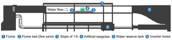
Figure 1.
Illustration of the experimental layout (not drawn to scale).
By varying the number of seagrasses, the row number, and the presence of adjacent objects, 14 experimental configurations were tested. Figure 2 illustrates each configuration: a single seagrass (Figure 2a), a single seagrass with an object (Figure 2b–d), two seagrasses in a row (Figure 2e), two seagrasses in different rows (Figure 2f), two seagrasses with an object (Figure 2g–j), three seagrasses in a row (Figure 2k), three seagrasses in different rows (Figure 2l), a medium seagrass meadow (Figure 2m), and a dense seagrass meadow (Figure 2n). Each object represents a natural or man-made structure (e.g., a rock or block) that may be present near seagrasses.
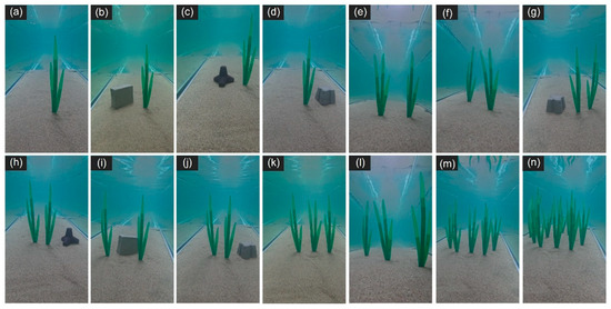
Figure 2.
Fourteen experimental configurations: (a) a single seagrass; (b–d) a single seagrass with an object; (e) two seagrasses in a row; (f) two seagrasses in different rows; (g–j) two seagrasses with an object; (k) three seagrasses in a row; (l) three seagrasses in different rows; (m) a medium seagrass meadow; and (n) a dense seagrass meadow.
A GoPro Hero 12 camera (GoPro Inc., San Mateo, CA, USA) was used to capture video footage. This device performs exceptionally well underwater. The camera supports 4K resolution and exhibits HyperSmooth stabilization, which ensures smooth footage even in rough conditions. During recording, the camera was moved to adjust the views of the seagrasses. It was positioned at varying distances from the seagrasses and moved to the right, left, upward, or downward to capture different perspectives. Each configuration was recorded at least twice in full high definition (FHD) at 30 frames per second. In total, 32 videos were obtained, from which images were extracted using Python 3.7 (Python Software Foundation; Wilmington, DE, USA). The extracted images measured 1920 pixels in height and 1080 pixels in width. At least two distinct images were selected from each video, captured from different viewpoints, resulting in a final set of 67 unique images.
It should be noted that the experimental setup was designed to mimic real ocean currents; accordingly, the feasibility of inducing the bending and vibration of the artificial seagrass was confirmed during the test. However, to ensure the clear image capture of the seagrass leaves and stems, the experiment was performed under low-turbidity (clear water) and no-turbulence conditions, which do not reflect realistic field conditions such as high turbidity and turbulent water.
2.2. Image Augmentation of the Experimental Dataset
Image augmentation is used to artificially expand a dataset [19]. This process increases the dataset size through geometric transformations (i.e., random flipping, rotation, cropping, scaling, and translation); color space augmentation (i.e., adjustment of brightness, contrast, saturation, and hue); noise injection (i.e., addition of Gaussian or salt-and-pepper noise to simulate real-world imperfections); cutout (i.e., random masking of rectangular regions in images); and mix-up (i.e., combination of two images and their labels to create new training samples) [20]. Database enrichment is widely applied in research. Some examples include the use of augmentation to increase the number of fish images [21] and the use of augmentation to randomly enhance an artificial reef dataset [22].
As shown in Figure 3, seven augmented versions of each of the original 67 images were generated by randomly selecting a rotation angle between −15 and 15 degrees and applying blurring, brightening, darkening, cropping, flipping, left rotation, and right rotation. This process yielded a total of 536 images, including both original and augmented versions. Similar dataset sizes have been considered reasonable in previous studies, including fish size estimation (562 images; [23]), the detection of a specific seagrass species (400 images; [24]), and the classification of polymeric microplastics on the sea surface (230 images; [25]). The dataset was divided into training and validation sets in the widely used 80:20 ratio [26,27]. Accordingly, 80% of the data (428 images) was allocated for training, whereas the remaining 20% (108 images) was reserved for validation. Generally, the use of both training and validation sets enhances model performance [28].
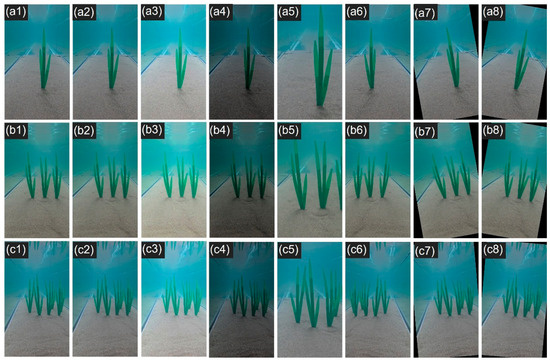
Figure 3.
Examples of the original images and their seven augmented versions: (a) a single seagrass; (b) three seagrasses in a row; and (c) a medium seagrass meadow. The notations (1–8) correspond, respectively, to the original image, a blurred image, a brightened image, a darkened image, a cropped image, a flipped image, a left-rotated image, and a right-rotated image.
2.3. Real Seagrass Dataset
Experimental datasets must exhibit high quality and resolution. However, underwater seagrass images often display poor quality, reducing accuracy. Image quality is influenced by water conditions, camera specifications, scene composition, and local environmental factors. The management of such issues is needed to increase the reliability of results.
Halophila stipulacea, a common seagrass species in the Red Sea, Indian Ocean, and Mediterranean Sea [29], was selected for testing. Real seagrass images were obtained from various sources on the internet. All selected images were sharp, included distinct seagrass stems, and depicted substantially different scenes. In total, 120 images (both original and augmented versions) were collected to create the real seagrass dataset.
2.4. Mask R-CNN
Mask R-CNN, a deep learning model, is an extension of the Faster R-CNN algorithm designed for both object detection and instance segmentation in computer vision. In the context of deep learning, a “model” refers to a mathematical representation or system developed to perform a specific task. Several studies (e.g., [30,31]) have provided comprehensive and detailed explanations of Mask R-CNN.
Figure 4 illustrates the framework of Mask R-CNN. The process begins when the backbone network generates a feature map from the input image [30]. This map captures details such as edges, textures, shapes, object parts, whole objects, and semantics. The region proposal network (RPN) then identifies potential regions of interest (RoIs). Within the RPN, a softmax function classifies anchors (predefined bounding boxes) into object and non-object categories; the bounding box regression (bbox reg) module refines these anchors by predicting offsets and scaling factors to ensure a better fit [32]. RoIAlign, an operator that extracts small feature maps from each RoI for detection and segmentation tasks, plays a crucial role in accurately extracting features from the feature map for each proposed region [31]. The Mask head, an additional branch of Mask R-CNN, generates segmentation masks for each RoI. Fully convolutional networks (FCNs) then utilize these mask predictions. The softmax function of the FCNs performs pixel-wise classification within the masks, normalizing scores to produce a probability distribution over classes for each pixel. This normalization enhances segmentation accuracy [31]. Finally, the bbox reg module of the FCNs further refines the bounding boxes of detected objects based on initial proposals generated by the RPN.
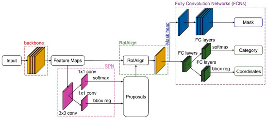
Figure 4.
Framework of Mask R-CNN.
In this study, we employed transfer learning to enhance the performance and efficiency of our seagrass and non-seagrass segmentation model. We initialized the Mask R-CNN model using pre-trained weights from the COCO dataset, which contains a wide variety of object categories. These weights retained the backbone’s general feature extraction capabilities—such as detecting edges, textures, and shapes. To adapt the model to our custom dataset, we replaced the original COCO classification and mask heads with new task-specific heads that were trained on annotated seagrass images. This approach enabled the model to leverage pre-learned visual features while refocusing its learning on our specific classes, thereby improving stability and effectiveness despite the limited training data. We trained the Mask R-CNN model using a ResNet-101 backbone, a learning rate of 0.001, a batch size of 2, and the Keras Stochastic Gradient Descent (SGD) optimizer with a momentum of 0.9 and a weight decay of 0.0001. The model was fine-tuned for 30 epochs, during which only the head layers were updated. Training was performed using an NVIDIA GeForce RTX 4060 Ti GPU with 8 GB of memory.
2.5. Evaluation Metrics
2.5.1. Loss
The loss function consists of three components: classification loss (), bounding box regression loss (), and mask loss () [21,30]. The classification loss measures the difference between the predicted and actual class labels. The bounding box regression loss evaluates the difference between the predicted and actual bounding box coordinates, whereas the mask loss quantifies the variance between the predicted and actual object masks. The total loss () is the sum of these three components [30]:
The detailed descriptions of each loss have been well documented in the literature [21,30,33,34,35]. For example, Figure 5 illustrates three types of boxes defined to evaluate the bounding box regression loss. The total loss serves as a metric for evaluating the performance of the deep learning model, with a particular focus on incorrect predictions. Lower loss values indicate improved model performance. Loss monitoring during training provides an initial assessment of the model. Additionally, loss tracking over time helps determine whether the model is converging (i.e., the loss stabilizes as the number of epochs increases). If convergence is observed, the model is considered well-trained.
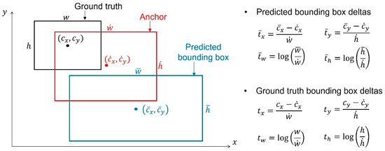
Figure 5.
The ground truth, anchor, and predicted bounding boxes, and their use in calculating the predicted and ground-truth bounding box deltas.
2.5.2. Intersection over Union
The IoU quantifies the overlap between the predicted bounding box and the ground-truth box via division of the overlapping area by the total area. An IoU score greater than 0.5 (or 50%) indicates that more than half of the predicted bounding box overlaps with the ground-truth box [21,36]. Figure 6 illustrates how specific IoU scores (0.9, 0.7, and 0.4) are identified for a single seagrass instance. The ground-truth bounding box is manually annotated and serves as a reference datum, whereas the predicted bounding box is generated by the trained model.
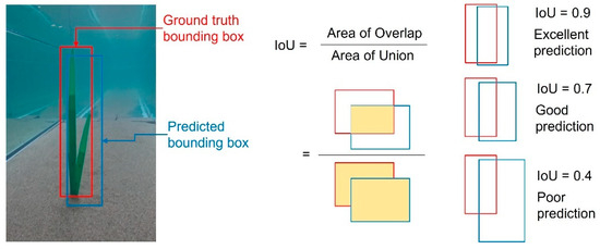
Figure 6.
Process for identifying IoU and some examples of IoU thresholds: a threshold of 0.9 is considered an excellent prediction, 0.7 is considered a good prediction, and 0.4 is considered a poor prediction.
2.5.3. Confusion Matrix
In classification tasks, particularly image recognition, several key outcomes are used to assess the performance of a trained model: true positive (TP), true negative (TN), false positive (FP), and false negative (FN). A TP occurs when the model correctly identifies the presence of an object, a TN when the model correctly predicts its absence, an FP when the model incorrectly predicts its presence, and an FN when the model fails to detect an object that is actually present, as illustrated in Figure 7. These outcomes are essential for evaluating model effectiveness because they influence key evaluation metrics, such as accuracy, precision, recall, and F1-score. Each evaluation metric has been well documented in the literature [21,24,37].
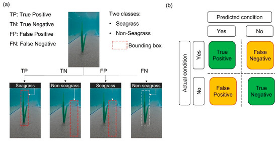
Figure 7.
Illustration of the four key outcomes: (a) TP, TN, FP, and FN for seagrass prediction; and (b) the confusion matrix consisting of the four key outcomes.
2.5.4. Evaluation Thresholds
It is often challenging to define reference values for the evaluation thresholds of metrics such as IoU, accuracy, precision, recall, and F1-score. These thresholds may vary depending on the application and individual researcher’s decisions. Therefore, benchmarks must be established to ensure that these metrics provide a standardized basis for evaluation. To address this need, we compiled the literature-recommended thresholds for five evaluation metrics (Table 1).

Table 1.
Thresholds for the five evaluation metrics.
There are no universally definitive thresholds. Most recommendations indicate that an IoU > 0.5 is acceptable; scores of approximately 0.7 are generally considered adequate for accuracy, precision, recall, and F1-score. Based on these recommendations, the IoU range was set to 0.5–1.0, whereas the ranges for other metrics were set to 0.7–1.0.
2.6. Frontal Area Estimation
This section describes the fundamental approach used to estimate the frontal area of seagrass leaves and stems. We utilized a dual-reference approach: one based on a reference object (M1) and the other on the distance between the camera and the seagrass (M2).
2.6.1. M1: Use of a Reference Object
Digital images are characterized by resolution. For example, a high-definition image has a resolution of 1280 × 720 pixels, where 1280 represents the number of horizontal pixels (width) and 720 denotes the number of vertical pixels (height). Thus, the total pixel area is 921,600 square pixels. Each object in the image occupies a specific pixel area. If both the pixel area of an object and the actual area represented by each pixel are known, the real area of seagrass in the image can be calculated. This concept is used to estimate the frontal area by incorporating a reference object.
First, images must contain both the seagrass and a reference object with a known area. Using the Mask R-CNN algorithm, both the reference object and the seagrass are detected, masks are generated as suggested by the model, and the mask shapes and areas are exported in pixels. A mask covers the surface of the object or seagrass; its area corresponds to the pixel area of the respective object. The conversion ratio is then calculated as the pixel area () divided by the actual area () of the reference object:
where is measured using a direct method, such as a ruler or an area meter. Because the conversion ratio (pixels/cm2) remains constant for all objects within the same image, the frontal area of the seagrass () can be determined from its pixel area (), as shown in Equation (2). Using this ratio, is derived, allowing for the estimation of the actual area of the seagrass. When the camera is positioned vertically above the flume bed to capture images perpendicular to the flow, the actual area of seagrass corresponds to the frontal area.
2.6.2. M2: Use of the Distance Between the Camera and Seagrass
The size of seagrass in an image varies depending on the distance between the seagrass and the camera. For example, when the camera is positioned closer, the seagrass appears larger, resulting in a greater pixel area. However, considering that a consistent relationship exists between the pixel area of the seagrass and the distance from the seagrass to the camera, this relationship can be utilized to estimate the frontal area of the seagrass.
First, the camera was calibrated to determine how the frontal area (cm2) corresponded to the pixel area in the image at a specific distance. This ratio was denoted as . During this step, a calibration image was obtained by capturing an image at a distance of 40 cm from a rectangular object measuring 4.8 cm in width and 4.9 cm in length, with a frontal area of 23.52 cm2. WebPlotDigitizer 4.5 (Automeris LLC, Frisco, TX, USA) was used to import this calibration image, create a polygon around the object, and extract the pixel area. The conversion ratio was calculated via the division of the frontal area (, cm2) by the pixel area ():
Next, to estimate the frontal area of seagrass, images were captured at a distance of 40 cm without a reference object. The frontal area () of seagrass was then estimated:
In the above calculation, the distance between the camera and the seagrass stem is required to be 40 cm. However, under practical conditions, it may not be possible to maintain this exact distance. Therefore, we have derived a method for accommodating an arbitrary distance. In Figure 8a, the calibration step is illustrated, with the camera positioned cm from the seagrass. In this step, the conversion ratio represents the ratio of the frontal area of the seagrass to its pixel area:
where and represent, respectively, the average height and width of the actual seagrass, and and denote the average height and width of the seagrass in the captured image.
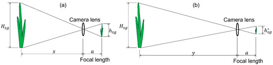
Figure 8.
A key concept for M2 (using the distance between the camera and seagrass): (a) calibration step and (b) measurement step.
Because the seagrass dimensions vary proportionally (i.e., ), we derive the following:
where denotes the focal length. By applying the triangle similarity as shown in Figure 8a, we derive the following:
Second, during the measurement step (see Figure 8b), we derive the following:
where denotes the seagrass height in the captured image. Accordingly, the ratio of any arbitrary distance to the calibration distance can be determined by the following:
By substituting from Equation (3e) into Equation (3h), we obtain the following:
Here, the term represents the conversion ratio at the arbitrary distance . Similarly, we can define for the arbitrary distance. Therefore, the relationship between the two conversion ratios, and , is given by the following:
Finally, we can estimate the seagrass frontal area as follows:
If , then , which corresponds to the scenario where the camera is positioned at the same distance from the seagrass. Overall, the process for M2 is categorized into three steps: calibration, measurement, and estimation. In the first step, the camera is positioned at a distance from the seagrass, an image is captured, and the conversion ratio is calculated. In the second step, the camera is placed at an arbitrary distance , a seagrass image is captured, and the conversion ratio is determined. In the final step, the seagrass frontal area is estimated using the equation .
3. Results
3.1. Total Loss
The total loss was evaluated after training with the experimental dataset. The model was trained for 400 epochs; each epoch consisted of 20 steps. The total loss for each epoch was calculated, as shown in Figure 9. The plot can be divided into two phases: a loss reduction phase and a convergence phase. During the loss reduction phase, the total loss decreases as the number of epochs increases. After 250 epochs, the total loss stabilizes, indicating the beginning of the convergence phase. Based on these results, the trained model from epoch 400 was used to detect seagrass.
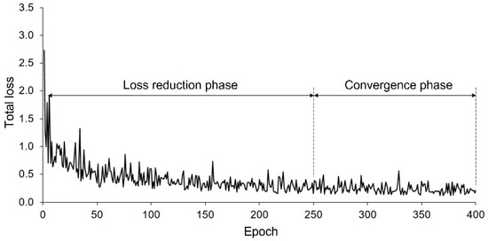
Figure 9.
Total loss for each epoch.
3.2. Model Metrics
Figure 10 presents the five evaluation metrics (IoU, precision, recall, accuracy, and F1-score) for the experimental dataset used in training, validation, and testing.
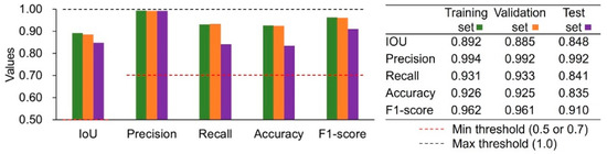
Figure 10.
Evaluation metrics for the experimental dataset: training set, validation set, and test set.
The maximum and minimum values of the upper and lower thresholds were selected with reference to Table 1. As shown in Figure 10, these values approach their respective maxima, indicating high model performance. Values in the test set are slightly lower than values in the training and validation sets. This discrepancy arises because the model was developed using the training set and fine-tuned based on the validation set. Additionally, the test set was utilized to revalidate the model, contributing to the slightly lower performance metrics observed in the test set.
3.3. Seagrass Detection
Figure 11 illustrates seagrass detection across 10 configurations: a single seagrass (Figure 11a), a single seagrass with an object (Figure 11b,c), two seagrasses (Figure 11d,e), two seagrasses with an object (Figure 11f), three seagrasses (Figure 11g,h), a medium seagrass meadow (Figure 11i), and a dense seagrass meadow (Figure 11j). In the medium seagrass meadow, seagrasses are closely spaced but rarely overlap in the captured images. In contrast, the dense seagrass meadow, which contains more seagrasses than the medium meadow, exhibits frequent overlapping in the captured images.
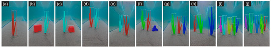
Figure 11.
Detection of seagrasses by the model: (a) a single seagrass; (b,c) a single seagrass with an object; (d,e) two seagrasses; (f) two seagrasses with an object; (g,h) three seagrasses; (i) a medium seagrass meadow; and (j) a dense seagrass meadow.
The model effectively detected a single seagrass (Figure 11a). The mask generated by the model covered almost the entire seagrass surface, although a small area at the bottom was omitted. In the previous section, we showed that the Mask R-CNN model recognizes features such as edges, textures, and shapes when identifying seagrasses. When these features were well-defined, the model accurately detected seagrasses. However, the lower part of the seagrass appeared dark due to shading and the presence of indistinct edges along the sandy flume bed. Thus, the model did not accurately detect the lower region.
Similarly, the model effectively detected a single seagrass with an object (Figure 11b,c), two seagrasses (Figure 11d,e), two seagrasses with an object (Figure 11f), and three seagrasses (Figure 11g,h). The masks generated by the model accurately covered the surfaces of the seagrasses and the object. However, the model did not fully capture the sharp tops of the seagrasses, hindering detection (Figure 11c,d). Additionally, the lower portions of the seagrasses in Figure 11d–g were not accurately detected.
For the medium seagrass meadow (Figure 11i), some portions of the seagrass leaves were not detected. However, the model performed well overall, covering most of the seagrass surfaces. In contrast, the dense seagrass meadow exhibited more undetected areas (Figure 11j) because the model relies on distinct edges, textures, and shapes for detection. When these features were clear (i.e., fewer seagrasses were present and overlap was minimal), the model readily detected the seagrasses. Conversely, when overlapping occurred and these features became less distinguishable, detection accuracy decreased. Therefore, when seagrasses did not overlap, the model effectively detected both single and multiple seagrasses.
3.4. Estimation of Seagrass Frontal Area
3.4.1. Estimation Using a Reference Object (M1)
To calculate the frontal area of a seagrass stem using a reference object (M1), a rectangular concrete object measuring 4.8 cm in width and 4.9 cm in height was selected as the reference. This object was placed next to the seagrass, an image was captured, and the frontal area of the seagrass stem was estimated based on the conversion ratio from Equation (2). Frontal area estimations were performed for five different seagrass stems, denoted SG1, SG2, SG3, SG4, and SG5. Additionally, two seagrass groups were considered: one comprising SG1 and SG2 and another comprising SG1, SG2, and SG3.
Figure 12 presents the bounding boxes and masks for a single seagrass with an object (Figure 12a–e), two seagrasses with an object (Figure 12f), and three seagrasses with an object (Figure 12g). To evaluate the accuracy of the areal estimation, the relative percentage error was calculated as follows:
where represents the actual measured frontal area and denotes the frontal area estimated by the model.
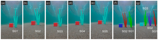
Figure 12.
Bounding boxes and masks for seagrasses obtained using a reference object (M1): panels (a–e) show a single seagrass with an object (SG1, SG2, SG3, SG4, or SG5); panel (f) shows two seagrasses (SG1 and SG2) with an object; and panel (g) shows three seagrasses (SG1, SG2, and SG3) with an object.
Table 2 presents the measured and estimated frontal areas for the seven images, along with the corresponding relative errors. All errors were less than 10%, indicating that the method achieved reasonable accuracy. A negative error indicates that the estimated area was larger than the measured area, whereas a positive error implies that the measured area was larger than the estimated area.
Table 2.
Measured and estimated frontal areas and relative percentage errors for seven seagrass images, determined using a reference object (M1).
The largest error occurred in Figure 12g, where the frontal areas of three seagrass stems were estimated simultaneously. Conversely, the smallest error was observed in Figure 12d, where only a single seagrass stem was assessed. These results suggest that the estimation accuracy depends on the number of seagrass stems analyzed. The estimation of a single stem’s frontal area was more accurate than the simultaneous estimation of multiple stems.
Notably, the measured and estimated frontal areas of the same seagrass varied across images. For example, the measured and estimated frontal areas for SG1 were 53.87 cm2 and 55.62 cm2 in Figure 12a, 47.67 cm2 and 49.10 cm2 in Figure 12f, and 51.75 cm2 and 47.77 cm2 in Figure 12g, respectively. These variations can be attributed to the flexible oscillations of seagrass in flowing water. Consequently, the frontal area of the seagrass changed across images, explaining the differences between measured and estimated values.
3.4.2. Estimation Using the Distance Between the Camera and Seagrasses (M2)
In this second method (M2), the distance between the camera and the seagrass was fixed at 40 cm, and the conversion ratio (7.88 × 10⁻⁴ cm2 per pixel) was determined during the calibration step. Seven images, similar to those used in the first method, were obtained. Figure 13 presents images of a single seagrass (SG1, SG2, SG3, SG4, or SG5), two seagrasses (SG1 and SG2), and three seagrasses (SG1, SG2, and SG3), including the corresponding bounding boxes and masks.
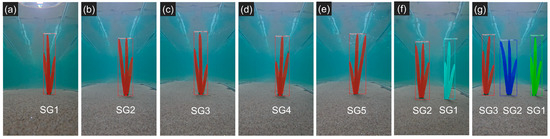
Figure 13.
Bounding boxes and masks for seagrasses obtained using the distance between the camera and seagrasses (M2): panels (a–e) show a single seagrass (SG1, SG2, SG3, SG4, or SG5); panel (f) shows two seagrasses (SG1 and SG2); and panel (g) shows three seagrasses (SG1, SG2, and SG3).
Table 3 displays the measured and estimated frontal areas of the seven seagrasses obtained using M2, along with the relative percentage errors. The maximum error was less than 10% (6.08% in Figure 13a), indicating that M2 was reasonably accurate. Unlike M1 (Figure 12), the accuracy of M2 was not significantly influenced by the number of seagrass stems analyzed.
Table 3.
Measured and estimated frontal areas and relative percentage errors for seven seagrass images, determined using the distance between the camera and seagrasses (M2).
3.5. Comparison of the Two Frontal Area Estimation Methods
Figure 14 compares relative percentage errors associated with the two frontal area estimation methods: the first method, which utilized a reference object, and the second method, which relied on the distance between the camera and the seagrass. The upper 10% limit represents the threshold at which the estimated frontal area is at most 10% larger than the measured frontal area. Similarly, the lower 10% limit indicates the threshold at which the estimated frontal area is at most 10% smaller than the actual measured frontal area. In Figure 14, the positive error range is 0% to 10%, indicating that the estimated area is smaller than the measured frontal area, whereas the negative error range is −10% to 0%, indicating that the estimated frontal area is larger than the measured frontal area. Overall, no significant difference in relative error was observed between the two methods. The maximum and minimum errors were similar (maximum: 7.68% vs. 6.08%; minimum: −0.43% vs. 1.44%). This result indicates that both methods exhibit comparable accuracy, and the selection of a specific method depends on the estimation conditions.
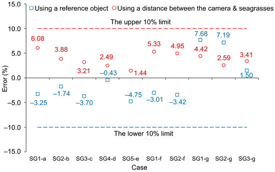
Figure 14.
Comparison of the relative percentage errors in estimating the frontal area of seagrasses using the dual-reference approach (M1 and M2). Note that the notation (e.g., SG1-a) indicates a specific configuration and its corresponding figure identification (Figure 11 and Figure 12), respectively.
3.6. Results of the Real Seagrass Dataset
After training with the real seagrass dataset, we obtained the evaluation metrics presented in Figure 15. These metrics include values for the training set and the validation set. The IoU, precision, and F1-score values all fell within the acceptable ranges for both datasets. However, differences in recall and accuracy were observed between the training and validation sets. Training set values were within the acceptable range, whereas validation set values were not. Nonetheless, validation set values (recall: 0.633; accuracy: 0.610) were very close to the lower limit (0.7).
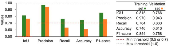
Figure 15.
Evaluation metrics for the real seagrass dataset: training set and validation set.
Compared with evaluation metrics for the experimental dataset (Figure 10), metrics for the real dataset (Figure 15) were less robust. This discrepancy can be attributed to differences in image resolution and quality. As previously noted, the real dataset, sourced from the internet, exhibited a lower image quality than the experimental dataset. Real dataset images were more blurred, of lower resolution, and less diverse (120 images compared with 536 images in the experimental dataset).
Consequently, the model trained on the real dataset did not accurately detect seagrass edges, textures, or shapes, leading to compromised seagrass detection. This poor model performance reduced the TP metric (seagrass was present and detected by the model) and increased the FN metric (seagrass was present but not detected by the model). The equations for accuracy, precision, recall, and the F1-score indicate that changes in TP and FN values lead to decreases in evaluation metric values. Regarding IoU values, the model trained on the real dataset did not accurately detect the edges of seagrasses, resulting in predicted bounding boxes that were smaller than the ground-truth bounding boxes. Consequently, IoU values were lower for the real dataset than for the experimental dataset.
Figure 16, Figure 17 and Figure 18 illustrate real seagrass detection. The images in Figure 16 and Figure 17 were used for training (i.e., part of the dataset used to generate the 120 images), whereas those in Figure 18 were excluded from training (i.e., an additional image set).
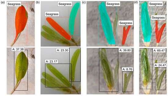
Figure 16.
Detection of real seagrasses taken in controlled environments and estimation of their pixel areas: (a) detection of a single seagrass leaf; (b) detection of four seagrass leaves—two clear and two blurred; and (c,d) detection of two seagrass leaves with sharp shapes or blurred regions (original images from [44,45]).
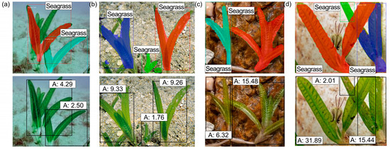
Figure 17.
Detection of real seagrasses captured in the ocean and estimation of their pixel areas on different seabeds (images used for training): (a) fine white sand seabed; (b) yellow and brown sand seabed; (c) brown seabed; and (d) white seabed with some organic waste (original images from [46,47,48,49]).
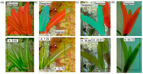
Figure 18.
Detection of real seagrasses captured in the ocean and estimation of their pixel areas under different conditions (images not used for training): (a) overlapping seagrass leaves and a blurred image; (b) a seabed with a color similar to that of seagrass; (c) a salt-and-pepper background; and (d) a blurred image (original images from [50,51]).
Moreover, the real images in Figure 17 were taken in controlled environments (e.g., in a laboratory), while those in Figure 18 and Figure 19 were taken in authentic seagrass environments. These classifications were intentionally made to test whether the proposed method works for real images in both controlled and authentic seagrass environments.
In Figure 16a, a clear seagrass leaf was successfully detected. However, in Figure 16b, although clear seagrass leaves were detected, two blurred leaves were missed. Similarly, the model accurately detected clear leaves but failed to detect those with sharp shapes or blurred regions (Figure 16c,d).
Figure 17 presents the results obtained using real seagrass images taken in different seabeds for testing. Overall, the model effectively detects the presence of seagrass; however, some areas in Figure 17a,b were not detected. This is mainly due to overlapping seagrass leaves and the small size of certain regions, which make them difficult to detect—an issue previously discussed in an earlier section. The masks align well with the seagrass surfaces, contributing to high accuracy in frontal area estimation, as the model calculates this area based on the generated masks. For further investigation, we also tested the model using additional images not included in the training set, as shown in Figure 18.
Figure 18 displays seagrass images captured under challenging conditions—such as motion blur (Figure 18a,b), low contrast between the seagrass and the background (Figure 18b,c), and salt-and-pepper noise (Figure 18b,c). These adverse conditions negatively impact the accuracy of the proposed method. As a result, the masks generated by the model do not align as well with the actual seagrass surfaces as those in Figure 16 and Figure 17. Specifically, in Figure 18a, the generated mask is larger than the actual seagrass region, while in Figure 18b, the mask fails to fully cover the seagrass surface. These examples not only highlight the significant influence of image capture quality on the model’s performance but also prompt the further refinement of the proposed method.
Figure 16, Figure 17 and Figure 18 also display the estimated pixel areas of detected seagrasses. Because these images were obtained from the internet, the conversion of pixel areas to frontal areas was not possible. To obtain frontal areas, information regarding a reference object in the images (M1) or the distance between the seagrass and the camera (M2) would be required. Overall, the Mask R-CNN model demonstrated applicability to real seagrass datasets. The dual-reference approach—using a reference object or the distance between the camera and the seagrass—may have practical value. However, model accuracy was highly dependent on image resolution, quality, and diversity within the dataset. In particular, the seagrass images captured under challenging conditions negatively impacted the accuracy of the proposed method. This highlights that additional tasks are required to increase the accuracy of the proposed method, such as increasing the size of the training dataset, incorporating images from more complex natural settings, and applying preprocessing techniques.
3.7. Applications of the Proposed Method
3.7.1. Estimation of Seagrass Bending Height
The deformation of flexible seagrass under the influence of currents or waves has garnered significant attention in recent years. For instance, Fonseca and Kenworthy [52] conducted lab-scale experiments with live vegetation subjected to unidirectional flow. Similarly, Luhar and Nepf [53] used a theoretical analysis to predict the bending height of a single artificial flexible vegetation stem in unidirectional flow. Zeller et al. [54] extended this research by performing lab-scale experiments with blade models under both wave and current conditions. Furthermore, Chau et al. [18] combined lab-scale experiments, Fluid–Structure Interaction (FSI) simulations, and a non-dimensional analysis to derive a regression equation for the seagrass bending height () under current conditions, as presented in Equation (5):
where is the seagrass height, is the seagrass width, is the seagrass thickness, is the density of seagrass, is the Young’s modulus, and is the flow velocity.
We considered seagrass samples made from polypropylene with representative density and Young’s modulus values, as shown in Table 4. The density of the samples ranges from 880 to 2400 kg m–3, with an average of 931 kg m–3, while the Young’s modulus varies between 0.008 and 8.25 GPa, with an average of 1.69 GPa [55]. Table 4 also presents the bending heights estimated using Equation (5), and the ratio is subsequently calculated. Since each seagrass stem consists of three leaves with varying widths from the base to the tip, the width and height values are averaged.
Table 4.
Seagrass samples and bending heights calculated using the regression equation proposed by Chau et al. [18]. The standard deviation (Std dev) for each category is provided for comparison.
Table 5 presents the vertical area of seagrass, measured using WebPlotDigitizer 4.5 (Automeris LLC, Frisco, TX, USA). In this process, an image of the seagrass in a vertical orientation was imported, and a polygon was drawn to enclose the entire seagrass surface. The area of this polygon represents the vertical area. The frontal area was calculated using the dual-reference approach (i.e., M1 and M2) proposed in this study.
Table 5.
Bending heights estimated using Mask R-CNN and the dual-reference approach (M1 and M2). The relative percentage differences in the ratio are calculated with respect to the values presented in Table 4. The standard deviation (Std dev) for each category is provided for comparison.
The ratio is equivalent to the ratio of the frontal area to the vertical area because the width of the seagrass stem remains constant during bending. The relative percentage differences in range from −1.63% to −10.16% for M1 and from −1.72% to −10.60% for M2 relative to the values in Table 4. This highlights that the bending height estimation by Mask R-CNN and the dual-reference approach represents the reduction in frontal area (or bending height) associated with seagrass bending behavior.
3.7.2. Estimation of Wave Height Reduction
The purpose of estimating the frontal area of flexible seagrass is to minimize overestimation when calculating parameters such as the drag coefficient, drag force, or wave height reduction in seagrass meadows. As previously discussed, most studies in the literature rely on the vertical area for these calculations due to the absence of exact methods for quantifying the frontal area. Traditional methods, such as using an area meter to measure the seagrass leaf area, provide only vertical area measurements. However, using the vertical area for such calculations tends to overestimate the functional capacity of seagrass.
To evaluate the impact of using the frontal area instead of the vertical area for calculating wave height reduction, we selected case studies from the experiments conducted by Losada et al. [56]. In their study, the authors developed an analytical formulation based on energy conservation to quantify the wave height downstream of a seagrass meadow, which was subsequently calibrated using a large-scale experiment. Table 6 presents the four cases from the experiment, while Table 7 details the seagrass properties used in the analysis. In the table, and represent the Young’s moduli of the seagrass stem and leaf, respectively, and the shoot density is defined as the number of seagrass shoots per unit area (m2).
Table 6.
Four investigated case studies.
Table 7.
Seagrass (Puccinellia maritima) properties.
In the previous section, we demonstrated that the ratio of the bending height to vertical height was similar between the dual-reference approach employed in this study and the correlation equation proposed by Chau et al. [18]. Given that the ratio is equivalent to the ratio of the frontal area to the vertical area—and considering that the Mask R-CNN estimation method could not be applied to the data from Losada et al. [56]—we employed the correlation equation proposed by Chau et al. [18] to quantify the frontal area based on bending height calculations.
To calculate the wave height, Losada et al. [56] developed an equation based on linear wave theory and energy conservation:
Here, is the downstream wave height measured at a distance (in meters) from the forefront of the seagrass meadow, is the upstream wave height, and is a damping factor. The damping factor is defined as follows:
Two coefficients, and , are defined by Equations (8) and (9), respectively:
where is the drag coefficient, is the shoot density, is the wave number, is the gravitational acceleration, and is the water depth. The wave number is determined by the dispersion relation:
where is the wave period.
We computed from Equations (7)–(9) and from Equation (6), taking into account the damping factor provided by Losada et al. [56]. Finally, the relative percentage difference in wave height was calculated as follows:
where is the wave height calculated using the vertical area, and is the wave height computed using the frontal area. Note that the use of and implies the use of and , respectively.
Figure 19 shows the ratio of downstream to upstream wave heights () for the four cases presented in Table 6. The ratio (depicted by blue circles in Figure 19) is consistently larger than (depicted by red triangles in Figure 19). This indicates that the seagrass meadow’s capacity to reduce the wave height is overestimated when is used to calculate . In other words, neglecting seagrass movement under water flow and wave conditions leads to an overestimation of the seagrass meadow’s effectiveness (by up to 9.23%).


Figure 19.
Ratio of downstream to upstream wave heights () for the four cases presented in Table 6: (a) case 1; (b) case 2; (c) case 3; and (d) case 4.
Figure 19.
Ratio of downstream to upstream wave heights () for the four cases presented in Table 6: (a) case 1; (b) case 2; (c) case 3; and (d) case 4.
Note that the drag force acting on an object is directly proportional to its frontal area, implying that a 10% error in estimating the frontal area results in a corresponding error in the drag coefficient. Moreover, according to Equations (6)–(9), a 10% error in estimating the frontal area affects the results through the coefficient via the drag coefficient . Consequently, the errors in and become 10%. For example, a fluctuation of in Equation (6) yields the following:
This indicates that the error in wave height reduction is . If we choose the median (0.2) of the damping factor ranges (0.1 to 0.3), the error in wave height reduction becomes 0.2%, 1.67%, 5.00%, 6.67%, and 9.52% for meadow lengths () of 0.1, 1, 5, 10, and 100 m, respectively. This estimation indicates that the error in wave height reduction can reach approximately 10% over a 100 m seagrass meadow when there is a 10% error in estimating the frontal area.
4. Discussion
Several studies have examined how flexible vegetation (e.g., seagrass) sways and bends under the influence of waves and water flow. For example, van Veelen et al. [57] reported that flexible vegetation attenuated waves by up to 70% less than rigid vegetation because the swaying of flexible plants reduced the frontal area, total work performed by the drag force, and total wave energy lost as waves moved over the vegetation. Liu et al. [58] conducted a laboratory-scale study and observed that rigid vegetation was more effective than flexible vegetation in reducing wave heights. Mullarney and Henderson [59] performed field experiments and found that wave dissipation increased with vegetation stem stiffness; overall dissipation by flexible stems was approximately 30% of that provided by rigid stems. Chau et al. [18] estimated the bending heights of flexible vegetation using particle image velocimetry, fluid–structure interaction simulations, and multiple regression analysis. The bending behavior of flexible vegetation reduced the wave height by approximately 10% less than that achieved with rigid vegetation. These studies highlight the fact that vegetation swaying and bending influence wave height reduction. However, all studies either assumed that the frontal area of vegetation remained constant, indirectly predicted the frontal area based on bending height, or did not explicitly measure the frontal area. For example, in the multiple regression analysis by Chau et al. [18], the bending height of vegetation was estimated and subsequently used to predict wave reduction.
We propose new approaches for measuring the frontal area of seagrass. In most configurations, the combination of the Mask R-CNN model and the dual-reference approach effectively segmented and quantified the frontal areas of seagrasses in underwater images. This approach enhances seagrass frontal area prediction accuracy by considering the bending of seagrasses in flowing water. Furthermore, because this indirect approach does not impact the environment, it may be preferable for seagrass-related research and applications. However, this study has several limitations and raises further considerations.
First, the performance of the proposed method is influenced by image quality, as evidenced by lower accuracy and recall values. This underscores the need to carefully control conditions during seagrass image capture. For instance, using water with low turbidity and minimal turbulence helps ensure clear images of the seagrass leaves, and selecting appropriate regions is crucial since accuracy decreases in areas with a high shoot density.
Second, water color also affects performance. Specifically, the method works best when there is a high contrast between the seagrass and the surrounding water. Moreover, the presence of animals or unfamiliar, straight objects in the images—elements not included in the model’s training data—can further reduce the method’s accuracy.
Third, under field conditions, various preprocessing techniques can be employed to improve the effectiveness of our method. Deblurring techniques help correct out-of-focus images via deconvolution, while contrast enhancement adjusts brightness levels to reveal hidden details in both dark and bright areas. Noise reduction methods may suppress salt-and-pepper noise while preserving important edges, and sharpening techniques can enhance image clarity by emphasizing fine details and boundaries. Additionally, color enhancement can adjust color intensity to ensure a better visual distinction of features, and super-resolution—using either deep learning models or interpolation—can upscale low-resolution images while recovering critical spatial information. We believe that incorporating these preprocessing steps can significantly enhance input data quality and, consequently, improve the accuracy, robustness, and reliability of the proposed method in practical field applications.
Fourth, in this study, we only considered water flow as the factor causing seagrass to bend and vibrate. However, under field conditions, wave motion also contributes to more complex seagrass movements. To incorporate the combined effects of water flow and wave motion, adjustments to the training dataset are necessary. In such cases, collecting sample data under both conditions—that is, water flow and wave motion—would allow the model to better learn the varying shapes of seagrass leaves, which, in turn, is expected to improve the segmentation accuracy of the model. We also consider this a potential direction for future work.
Fifth, the dataset comprises only 120 real seagrass images, limiting both the diversity and volume of data available for robust performance evaluation. Additionally, the lack of ground-truth area measurements—owing to the images being sourced online—reduces the precision with which segmentation accuracy can be validated. Although real seagrass images were incorporated, most images primarily reflect close-up, laboratory-style conditions rather than true in situ underwater environments. This discrepancy, as illustrated in Figure 17 and Figure 18, calls for further investigation into how to improve the accuracy of seagrass detection—for example, by increasing the size of the training dataset, incorporating images from more complex natural settings, and applying preprocessing techniques.
Finally, the distance-based method (M2) requires knowing the exact distance between the camera and the seagrass, necessitating a thin, lightweight ruler or measuring stick. In dynamic field conditions, achieving this precision can be challenging. This method also assumes that the lens’s focal length is fixed; however, minor variations in equipment or environment can induce measurement errors. Additionally, optical distortions—such as refraction—are only partly corrected by positioning the camera perpendicular to the seagrass bed or using flat port housings. Maintaining a constant camera-to-seagrass distance is difficult in uneven terrains, and while an alternative reference-object method (M1) is suggested, natural variability may still hinder accurate segmentation and area estimation. Thus, although promising under controlled conditions, the method requires the further development of robust measurement protocols and optical compensation techniques for broader, real-world applicability.
5. Conclusions
In this study, we developed an indirect method for detecting seagrasses and estimating their frontal areas by combining the Mask R-CNN model with a dual-reference approach. A laboratory-scale experiment using an underwater camera generated an experimental dataset that was divided into training, validation, and test sets. After training, evaluation metrics—including IoU, accuracy, precision, recall, and F1-score—approached their upper limits and remained within acceptable ranges. The model was further validated using real seagrass images; although the evaluation metrics were somewhat lower than those observed in the experimental dataset, performance remained satisfactory. However, seagrass images captured under challenging conditions (i.e., authentic seagrass environment)—such as motion blur, low contrast between the seagrass and the background, and salt-and-pepper noise—negatively impact the accuracy of the proposed method. This not only underscores the significant influence of image capture quality on the model’s performance but also calls for the further refinement of the proposed method. The proposed method was then employed to estimate the frontal areas of seagrasses, yielding errors below 10% (with a maximum of 7.68% and a minimum of –0.43%), thereby demonstrating high performance. Overall, the frontal area estimation using the proposed method exhibited improved accuracy by incorporating the bending of seagrasses under flowing water conditions. Moreover, we demonstrated that the indirect measurement of the seagrass frontal area significantly influences the estimation of the seagrass bending height and the capacity for wave height reduction, thereby mitigating the overestimation associated with traditional direct methods. Accordingly, the indirect approach shows promise for future applications, as it is environmentally friendly and overcomes the limitations inherent in existing direct measurement techniques.
Author Contributions
Conceptualization, T.V.C. and W.-B.N.; methodology, T.V.C.; software, T.V.C.; validation, S.J., M.K., and W.-B.N.; formal analysis, T.V.C. and M.K.; investigation, T.V.C., S.J., and M.K.; resources, S.J. and M.K.; data curation, T.V.C.; writing—original draft preparation, T.V.C.; writing—review and editing, W.-B.N.; visualization, T.V.C. and S.J.; supervision, W.-B.N.; project administration, S.J. and W.-B.N.; funding acquisition, W.-B.N. All authors have read and agreed to the published version of the manuscript.
Funding
This research was supported by Basic Science Research Program through the National Research Foundation of Korea (NRF) funded by the Ministry of Education (2021R1I1A3048650).
Data Availability Statement
The original contributions presented in this study are included in the article. Further inquiries can be directed to the corresponding author.
Conflicts of Interest
The authors declare no conflicts of interest.
References
- Duarte, C.M. The future of seagrass meadows. Environ. Conserv. 2002, 29, 192–206. [Google Scholar] [CrossRef]
- Orth, R.J.; Carruthers, T.J.B.; Dennison, W.C.; Duarte, C.M.; Fourqurean, J.W.; Heck, K.L.; Hughes, A.R.; Kendrick, G.A.; Kenworthy, W.J.; Olyarnik, S.; et al. A global crisis for seagrass ecosystems. Bioscience 2006, 56, 987–996. [Google Scholar] [CrossRef]
- Waycott, M.; Duarte, C.M.; Carruthers, T.J.B.; Orth, R.J.; Dennison, W.C.; Olyarnik, S.; Calladine, A.; Fourqurean, J.W.; Heck, K.L.; Hughes, A.R.; et al. Accelerating loss of seagrasses across the globe threatens coastal ecosystems. Proc. Natl. Acad. Sci. USA 2009, 106, 12377–12381. [Google Scholar] [CrossRef] [PubMed]
- Chau, V.T. Vision Image and Mask RCNN-Based Estimation of Frontal Area of Seagrass for Coastal Protection Function. Ph.D. Thesis, Pukyong National University, Busan, Republic of Korea, 2025; pp. 1–180. [Google Scholar]
- Kobayashi, N.; Raichle, A.; Asano, T. Wave attenuation by vegetation. J. Waterw. Port Coast. Ocean. Eng. 1993, 119, 30–48. [Google Scholar] [CrossRef]
- Paul, M.; Bouma, T.J.; Amos, C.L. Wave attenuation by submerged vegetation: Combining the effect of organism traits and tidal current. Mar. Ecol. Prog. Ser. 2012, 444, 31–41. [Google Scholar] [CrossRef]
- Twomey, A.J.; O’Brien, K.R.; Callaghan, D.P.; Saunders, M.I. Synthesising wave attenuation for seagrass: Drag coefficient as a unifying indicator. Mar. Pollut. Bull. 2020, 160, 111661. [Google Scholar] [CrossRef]
- Phillips, R.C.; McRoy, C.P. Seagrass Research Methods; United Nations Educational, Scientific and Cultural Organization: Paris, France, 1990. [Google Scholar]
- Short, F.T.; Duarte, C.M. Methods for the measurement of seagrass growth and production. In Global Seagrass Research Methods; Elsevier Science: Amsterdam, The Netherlands, 2001; pp. 155–182. [Google Scholar] [CrossRef]
- Short, F.T.; Coles, R.G.; Short, C.A. SeagrassNet Manual for Scientific Monitoring of Seagrass Habitat; Worldwide edition; University of New Hampshire Publication: Durham, NH, USA, 2015. [Google Scholar]
- Riniatsih, I.; Ambariyanto, A.; Yudiati, E.; Redjeki, S.; Hartati, R. Monitoring the seagrass ecosystem using the unmanned aerial vehicle (UAV) in coastal water of Jepara. IOP Conf. Ser. Earth Environ. Sci. 2021, 674, 012075. [Google Scholar] [CrossRef]
- Paul, M.; Lefebvre, A.; Manca, E.; Amos, C.L. An acoustic method for the remote measurement of seagrass metrics. Estuar. Coast. Shelf Sci. 2011, 93, 68–79. [Google Scholar] [CrossRef]
- Morsy, S.; Suárez, A.B.Y.; Robert, K. 3D Mapping of Benthic Habitat Using XGBoost and Structure from Motion Photogrammetry. ISPRS Ann. Photogramm. Remote Sens. Spat. Inf. Sci. 2023, 10, 1131–1136. [Google Scholar] [CrossRef]
- Komatsu, T.; Igararashi, C.; Tatsukawa, K.; Nakaoka, M.; Hiraishi, T.; Taira, A. Mapping of seagrass and seaweed beds using hydro-acoustic methods. Fish. Sci. 2002, 68, 580–583. [Google Scholar] [CrossRef][Green Version]
- Fonseca, M.S.; Koehl, M.A.R.; Kopp, B.S. Biomechanical factors contributing to self-organization in seagrass landscapes. J. Exp. Mar. Biol. Ecol. 2007, 340, 227–246. [Google Scholar] [CrossRef]
- Clarke, S.J. Vegetation growth in rivers: Influences upon sediment and nutrient dynamics. Prog. Phys. Geogr. 2002, 26, 159–172. [Google Scholar] [CrossRef]
- Rovira, A.; Alcaraz, C.; Trobajo, R. Effects of plant architecture and water velocity on sediment retention by submerged macrophytes. Freshw. Biol. 2016, 61, 758–768. [Google Scholar] [CrossRef]
- Chau, V.T.; Jung, S.; Kim, M.; Na, W.B. Analysis of the Bending Height of Flexible Marine Vegetation. J. Mar. Sci. Eng. 2024, 12, 1054. [Google Scholar] [CrossRef]
- Nanthini, K.; Sivabalaselvamani, D.; Chitra, K.; Gokul, P.; KavinKumar, S.; Kishore, S. A Survey on Data Augmentation Techniques. In Proceedings of the 2023 7th International Conference on Computing Methodologies and Communication (ICCMC), Erode, India, 23–25 February 2023; pp. 913–920. [Google Scholar]
- Shorten, C.; Khoshgoftaar, T.M. A survey on Image Data Augmentation for Deep Learning. J. Big Data 2019, 6, 60. [Google Scholar] [CrossRef]
- Conrady, C.R.; Er, Ş.; Attwood, C.G.; Roberson, L.A.; de Vos, L. Automated detection and classification of southern African Roman seabream using mask R-CNN. Ecol. Inform. 2022, 69, 101593. [Google Scholar] [CrossRef]
- Song, Y.; Wu, Z.; Zhang, S.; Quan, W.; Shi, Y.; Xiong, X.; Li, P. Estimation of Artificial Reef Pose Based on Deep Learning. J. Mar. Sci. Eng. 2024, 12, 812. [Google Scholar] [CrossRef]
- Álvarez-Ellacuría, A.; Palmer, M.; Catalán, I.A.; Lisani, J.L. Image-based, unsupervised estimation of fish size from commercial landings using deep learning. ICES J. Mar. Sci. 2020, 77, 1330–1339. [Google Scholar] [CrossRef]
- Lestari, N.A.; Jaya, I.; Iqbal, M. Segmentation of seagrass (Enhalus acoroides) using deep learning mask R-CNN algorithm. IOP Conf. Ser. Earth Environ. Sci. 2021, 944, 012015. [Google Scholar] [CrossRef]
- Thammasanya, T.; Patiam, S.; Rodcharoen, E.; Chotikarn, P. A new approach to classifying polymer type of microplastics based on Faster-RCNN-FPN and spectroscopic imagery under ultraviolet light. Sci. Rep. 2024, 14, 3529. [Google Scholar] [CrossRef]
- Abdulrazzaq, M.M.; Yaseen, I.F.T.; Noah, S.A.; Fadhil, M.A. Multi-level of feature extraction and classification for X-ray medical image. Indones. J. Electr. Eng. Comput. Sci. 2018, 10, 154–167. [Google Scholar] [CrossRef]
- Joseph, V.R. Optimal ratio for data splitting. Stat. Anal. Data Min. 2022, 15, 531–538. [Google Scholar] [CrossRef]
- Bishop, C.M. Pattern Recognition and Machine Learning; Springer: New York, NY, USA, 2006; pp. 1–675. ISBN 978-0387-31073-2. [Google Scholar]
- Thibaut, T.; Blanfuné, A.; Boudouresque, C.F.; Holon, F.; Agel, N. Distribution of the seagrass Halophila stipulacea: A big jump to the northwestern Mediterranean Sea. Aquat. Bot. 2022, 176, 103465. [Google Scholar] [CrossRef]
- He, K.; Gkioxari, G.; Dollár, P.; Girshick, R. Mask R-CNN. In Proceedings of the 2017 IEEE International Conference on Computer Vision, Venice, Italy, 22–29 October 2017; pp. 2980–2988. [Google Scholar] [CrossRef]
- Potrimba, P. What Is Mask R-CNN? The Ultimate Guide. Available online: https://blog.roboflow.com/mask-rcnn/ (accessed on 1 June 2024).
- Fang, S.; Zhang, B.; Hu, J. Improved Mask R-CNN Multi-Target Detection and Segmentation for Autonomous Driving in Complex Scenes. Sensors 2023, 23, 3853. [Google Scholar] [CrossRef]
- Girshick, R. Fast R-CNN. In Proceedings of the 2015 IEEE International Conference on Computer Vision, Santiago, Chile, 7–13 December 2015; pp. 1440–1448. [Google Scholar] [CrossRef]
- Ren, S.; He, K.; Girshick, R.; Sun, J. Faster R-CNN: Towards Real-Time Object Detection with Region Proposal Networks. arXiv 2015, arXiv:1506.01487. [Google Scholar] [CrossRef]
- Cha, Y.J.; Choi, W.; Suh, G.; Mahmoudkhani, S.; Büyüköztürk, O. Autonomous Structural Visual Inspection Using Region-Based Deep Learning for Detecting Multiple Damage Types. Comput. Civ. Infrastruct. Eng. 2017, 33, 731–747. [Google Scholar] [CrossRef]
- Rosebrock, A. Deep Learning for Computer Vision with Python; PyImageSearch: Philadelphia, PA, USA, 2017; pp. 29–140. [Google Scholar]
- Christen, R.; Hand, D.J.; Kirielle, N. A review of the F-measures: Its history, properties, criticism, and alternatives. ACM Comput. Surv. 2023, 56, 73. [Google Scholar] [CrossRef]
- Everingham, M.; Van Gool, L.; Williams, C.K.I.; Winn, J.; Zisserman, A. The pascal visual object classes (VOC) challenge. Int. J. Comput. Vis. 2010, 88, 303–338. [Google Scholar] [CrossRef]
- Lin, T.Y.; Maire, M.; Belongie, S.; Hays, J.; Perona, P.; Ramanan, D.; Dollár, P.; Zitnick, C.L. Microsoft COCO: Common Objects in Context. In Proceedings of the Computer Vision—EECV 2014. EECV 2014. Lecture Notes in Computer Science, Zurich, Switzerland, 6–12 September 2014; Fleet, D., Pajdla, T., Schiele, B., Tuytelaars, T., Eds.; Springer: Cham, Switzerland, 2014; pp. 740–755. [Google Scholar] [CrossRef]
- Boesch, G. What Is Intersection over Union (IoU)? Available online: https://viso.ai/computer-vision/intersection-over-union-iou/ (accessed on 5 July 2024).
- Cloudfactory, Confusion Matrix. Available online: https://wiki.cloudfactory.com/docs/mp-wiki/metrics/confusion-matrix (accessed on 1 December 2024).
- Barkved, K. How to Know If Your Machine Learning Model Has Good Performance. Available online: https://www.obviously.ai/post/machine-learning-model-performance (accessed on 15 January 2025).
- Logunova, I. A Guide to F1 Score. Available online: https://serokell.io/blog/a-guide-to-f1-score (accessed on 1 January 2025).
- Sergeev, A. Halophila Ovalis (R.Br.) Hook.f. Available online: https://www.floraofqatar.com/halophila_ovalis.htm (accessed on 1 June 2024).
- Mifsud, S. Halophila Stipulacea (Halophila Seagrass). Available online: https://www.maltawildplants.com/HYCH/Halophila_stipulacea.php (accessed on 1 June 2024).
- Okudan, E.Ş.; Dural, B.; Demir, V.; Erduğan, H.; Aysel, V. Biodiversity of marine benthic macroflora (seaweeds/macroalgae and seagrasses) of the Mediterranean Sea. In The Turkish Part of the Mediterranean Sea: Marine Biodiversity, Fisheries, Conservation and Governance; Publication No: 43; Turan, G., Salihoğlu, B., Özbek, E.Ö., Öztürk, B., Eds.; Turkish Marine Research Foundation (TUDAV): Istanbul, Turkey, 2016; pp. 107–135. ISBN 978-9-7588-2535-6. [Google Scholar]
- Algae Base, Zostera Stipulacea Forsskål 1775. Available online: https://www.algaebase.org/search/species/detail/?species_id=65451 (accessed on 1 June 2024).
- Sergeev, A. Algae Base, Seagrass (Halophila stipulacea) in Purple Island (Jazirat Bin Ghanim). Al Khor, Qatar, 9 October 2014. Available online: https://www.asergeev.com/pictures/archives/compress/2014/1488/13s.htm (accessed on 1 June 2024).
- Mittelmeer- und Alpenflora. Gattung: Halophila (Seagrass). Available online: https://www.mittelmeerflora.de/Einkeim/Hydocharitaceae/halophila.htm (accessed on 1 June 2024).
- Biologiamarina org. Halophila Stipulacea, Alofila. Available online: https://www.biologiamarina.org/halophila-stipulacea/ (accessed on 20 June 2025).
- iNaturalist. Halophila Stipulacea. Available online: https://inaturalist.ca/taxa/131137-Halophila-stipulacea/browse_photos (accessed on 20 June 2025).
- Fonseca, M.S.; Kenworthy, W.J. Effects of current on photosynthesis and distribution of seagrasses. Aquat. Bot. 1987, 27, 59–78. [Google Scholar] [CrossRef]
- Luhar, M.; Nepf, H.M. Flow-induced reconfiguration of buoyant and flexible aquatic vegetation. Limnol. Oceanogr. 2011, 56, 2003–2017. [Google Scholar] [CrossRef]
- Zeller, R.B.; Weitzman, J.S.; Abbett, M.E.; Zarama, F.J.; Fringer, O.B.; Koseff, J.R. Improved parameterization of seagrass blade dynamics and wave attenuation based on numerical and laboratory experiments. Limnol. Oceanogr. 2014, 59, 251–266. [Google Scholar] [CrossRef]
- Matweb. Material Property Data. Overview of Materials for Polypropylene, Molded. Available online: https://www.matweb.com/search/datasheet.aspx?MatGUID=08fb0f47ef7e454fbf7092517b2264b2&ckck=1 (accessed on 9 March 2025).
- Losada, I.J.; Maza, M.; Lara, J.L. A new formulation for vegetation-induced damping under combined waves and currents. Coast. Eng. 2016, 107, 1–13. [Google Scholar] [CrossRef]
- van Veelen, T.J.; Fairchild, T.P.; Reeve, D.E.; Karunarathna, H. Experimental study on vegetation flexibility as control parameter for wave damping and velocity structure. Coast. Eng. 2020, 157, 103648. [Google Scholar] [CrossRef]
- Liu, S.; Xu, S.; Yin, K. Optimization of the drag coefficient in wave attenuation by submerged rigid and flexible vegetation based on experimental and numerical studies. Ocean Eng. 2023, 285, 115382. [Google Scholar] [CrossRef]
- Mullarney, J.C.; Henderson, S.M. Wave-forced motion of submerged single-stem vegetation. J. Geophys. Res. Oceans 2010, 115, C12061. [Google Scholar] [CrossRef]


Disclaimer/Publisher’s Note: The statements, opinions and data contained in all publications are solely those of the individual author(s) and contributor(s) and not of MDPI and/or the editor(s). MDPI and/or the editor(s) disclaim responsibility for any injury to people or property resulting from any ideas, methods, instructions or products referred to in the content. |
© 2025 by the authors. Licensee MDPI, Basel, Switzerland. This article is an open access article distributed under the terms and conditions of the Creative Commons Attribution (CC BY) license (https://creativecommons.org/licenses/by/4.0/).