Article

Uncertainty-Guided Prediction Horizon of Phase-Resolved Ocean Wave Forecasting Under Data Sparsity: Experimental and Numerical Evaluation

by
Yuksel Rudy Alkarem
1,
Kimberly Huguenard
1,
Richard W. Kimball
2 and
Stephan T. Grilli
3,*
1
Civil and Environmental Engineering Department, University of Maine, 35 Flagstaff Road, Orono, ME 04469, USA
2
Mechanical Engineering Department, University of Maine, 35 Flagstaff Road, Orono, ME 04469, USA
3
Department of Ocean Engineering, University of Rhode Island, Narragansett, RI 02882, USA
*
Author to whom correspondence should be addressed.
J. Mar. Sci. Eng. 2025, 13(7), 1250; https://doi.org/10.3390/jmse13071250
Submission received: 5 June 2025 / Revised: 18 June 2025 / Accepted: 25 June 2025 / Published: 28 June 2025
(This article belongs to the Special Issue Data-Driven Methods for Marine Structures)

Abstract

Accurate short-term wave forecasting is critical for the safe and efficient operation of marine structures that rely on real-time, phase-resolved ocean wave information for control and monitoring purposes (e.g., digital twins). These systems often depend on environmental sensors (e.g., waverider buoys, wave-sensing LIDAR). Challenges arise when upstream sensor data are missing, sparse, or phase-shifted due to drift. This study investigates the performance of two machine learning models, time-series dense encoder (TiDE) and long short-term memory (LSTM), for forecasting phase-resolved ocean surface elevations under varying degrees of data degradation. We introduce the τ -trimming algorithm, which adapts the prediction horizon based on uncertainty thresholds derived from historical forecasts. Numerical wave tank (NWT) and wave basin experiments are used to benchmark model performance under short- and long-term data masking, spatially coarse sensor grids, and upstream phase shifts. Results show under a 50% probability of upstream data loss, the τ -trimmed TiDE model achieves a 46% reduction in error at the most upstream target, compared to 22% for LSTM. Furthermore, phase misalignment in upstream data introduces a near-linear increase in forecast error. Under moderate model settings, a ±3 s misalignment increases the mean absolute error by approximately 0.5 m, while the same error is accumulated at ±4 s using the more conservative approach. These findings inform the design of resilient, uncertainty-aware wave forecasting systems suited for realistic offshore sensing environments.

1. Introduction

Ocean waves exert significant forces on offshore structures, potentially inducing large motions in floating systems that affect both operational efficiency and fatigue life. Predicting wave propagation in space and time is the focus of many studies, using a variety of both physics-based and, more recently, data-driven models. Away from shore, irregular ocean waves have typically been represented by linear superposition, leading to a spectral representation in the frequency domain, with related spectral and statistical parameters (e.g., significant wave height, peak spectral period, etc). This approach helps determine, or forecast, extreme sea-state parameters for various analyses and design purposes. However, a spectral representation lacks phase, i.e., individual wave information, which becomes extremely important for many applications such as optimizing motion control strategies of a floating structure. For example, Li et al. [1] concluded that wave energy converters have increased efficiency when their control mechanism assimilates phase-resolved wave predictions. In the context of floating wind systems, phase-resolved predictions are essential for the development of active control strategies and digital twin frameworks. Alkarem et al. [2] conducted reconstruction and forecast of floater’s motion supporting a wind turbine under the assumptions that upstream wave information and wave prediction–reconstruction models are available and reliable to reconstruct wave fields near the floating platform. Albertson et al. [3] validated three wave reconstruction prediction models: a linear wave theory (LWT)-based model with a wave dispersion corrected for nonlinearity and a 2 n d -order wave model with nonlinear dispersive properties initialized by a linear prediction, against fully nonlinear potential flow simulations. The models appeared to provide reasonable short-term predictions at the float that can later be used for real-time control of float motions using a moving mass or ballast. Beyond renewable energy applications, seaborne additive manufacturing (SAM) [4] and underwater 3D printing [5] are other examples where the short-term phase-resolved predictions are crucial to ensure accurate operations at sea.
Physics-based predictions of ocean wave fields require using a physically relevant model and “inverting” it to fit it to observations (i.e., by minimizing the mean square error of simulated to measured), e.g., [3,6]. This is called the nowcast. Once a nowcast of the ocean surface is obtained on the basis of some measurements, the fitted model can then be used to perform a forecast of the wave surface elevation expected at the location and future time of interest [7]. Desmars et al. [8] validated the use of this algorithm, both numerically and experimentally, using non-uniformly distributed wave gauges, representing a spatial sampling using an optical sensor (e.g., LIDAR). They confirmed that the prediction accuracy converged as the amount of input data involved during the inversion process increased. Naaijen and Huijsmans [9] compared wave elevation predicted by their model against measured wave elevations at various distances downstream for different wave conditions and showed that the prediction horizon can be extended further than the theoretical limits. For models based on LWT, the predictable space–time zone can be determined based on the wave group velocities of the fastest and slowest components of the reconstructed wave field [10]. Qi et al. [11] investigated the variation of the theoretical phase-resolved predictable zone in space–time for multi-directional irregular wave fields and considered optimal deployment to maximize predictable zone space–time volume.
For severe sea-states, more advanced wave models have been developed that account for wave nonlinearity (to some order), which affects both wave shape and phase speed, e.g., [8,12,13,14] For instance, Grilli et al. [6] and Nouguier et al. [13] developed nonlinear free surface reconstruction algorithms, using an efficient Lagrangian-based choppy model [12] and the improved, hybrid variation [14] and validated them for 1D and 2D irregular surface waves, using simulated LIDAR data to create relevant data sets. More recently, Kim et al. [15] conducted experiments and validated these models using 2D data, concluding that accurate wave forecasting in multidirectional seas, compared to that in unidirectional seas, requires accounting for both directional and frequency components of the wave field.
While physics-based models can achieve near real-time reconstruction and predictions as long as nonlinear effects are weak or negligible [3,15,16,17], the reconstruction problem (i.e., determining the state of the wave field, wave components, nonlinear couplings, etc.) and the time it takes to invert, integrate equations, and generate predictions are major challenges to the practicality of using such models in severe sea-states [18], unless powerful computational hardware is embarked onto the marine structure. As an alternate approach, advanced machine learning tools, when properly trained on relevant data, have promising potential to accelerate these processes and even enhance the accuracy of the predictions [19]. For instance, the proposed model by Zhang et al. [20], which is based on a variational Bayesian machine learning approach, outperformed conventional models in terms of prediction accuracy by reducing the error as much as 55% and length of the predictable zone by expanding it by as much as 74%. Jörges et al. [21] used long short-term memory (LSTM), a recursive neural network (RNN) type, to predict nearshore significant wave heights. Mohaghegh et al. [18] investigated a machine learning technique that accurately handles wave predictions with more than two orders of magnitude quicker than numerically solving governing equations. Kagemoto [22] developed a LSTM model to predict experimental and numerical irregular wave trains and extrapolated their model to forecast the motion response of a floating body. They concluded that the model is capable of producing reasonably accurate predictions in spite of nonlinear effects present in the data. Duan et al. [23] constructed a neural-network-based wave prediction model (ANN-WP) where they utilized experimental data to train, validate, and conduct comparison studies with linear wave prediction (LWP) algorithms and proved that ANN-WP is superior in performance to LWP.
Zhang et al. [20] demonstrated that uncertainty quantification (UQ) can be used in conjunction with phase-resolved real-time wave prediction to (1) expand the predictable zone, which is otherwise quite conservative when using LWT-based models; (2) inform the control algorithm of the level of confidence to perform a control action based on an uncertainty score for a given predicted value. Silva and Maki [24] applied similar uncertainty quantification using the Monte Carlo dropout approach proposed by Gal and Ghahramani [25] to perform system identification for 6-DOF ship motions in waves under various upstream wave probe setups. Law et al. [26] used a higher-order spectral–numerical wave tank (HOS-NWT) method developed by Bonnefoy et al. [27] and Ducrozet et al. [28] to generate datasets to train their artificial neural network for two wave steepness values, a limiting and a mean steepness value. Harris [29] developed a data-driven model that is faster than real-time. Their choice of machine learning approach was the time-series dense encoder (TiDE) as it has shown good balance between model complexity, stability, and computational time. Li et al. [30] developed a three-dimensional, phase-resolved ocean wave forecast based on a wave tank experiment where they used various machine learning methods including recursive and convolutional neural networks.
Even though prior research efforts demonstrated that machine learning (ML) models can generate accurate and rapid forecasts of phase-resolved ocean wave fields, primarily through numerical simulations, e.g., [18,22,23,24,26] and, to a lesser extent, through experimental validation, e.g., [15,29,30], limited attention is paid to their resilience and generalizability under realistic offshore sensing conditions. Additionally, the number and placement of upstream wave probes in these studies are fixed and highly controlled, e.g., [23,26,31]. In contrast, real-world deployments, particularly in deep water, often involve dynamic or uncertain probe locations due to drifting buoys. To the author’s knowledge, the research conducted by Qi et al. [11] was the only study where an analytical LWT-based predictable zone was derived based on moving measured probes and their reconstruction method validated in their subsequent publication [32]. However, no uncertainty assessment was conducted on the predictable zone induced by moving probes. Upstream data could become unavailable due to shadowing effects or occlusion in optical measurements due to low visibility or splashing. These variations can significantly alter the spatial distribution of the available data used for wave reconstruction. The issue is further exacerbated when optical sensors such as LIDARs are employed. Data loss may also occur due to equipment malfunction, shadowing effects, or the inability to detect the free surface location reliably. Despite these challenges being common in practical applications, and despite the increasing use of ML-models, the impact of data sparsity and phase misalignment on forecast quality remains underexplored, particularly for experimental datasets.
To address these gaps, the present work evaluates the performance and resilience of ML-based wave field reconstruction methods under realistic, variable data acquisition scenarios. In the context of this paper, a model’s resilience is defined by the model’s ability to maintain acceptable performance despite uncertain or incomplete input. Specifically, we selected two ML-models; LSTM and TiDE. The LSTM model is extensively used for the reconstruction and prediction of time-series in various related fields such as the work of Jörges et al. [21] but has also been reported to have higher prediction error compared to other advanced models [30]. The TiDE model, as validated by Harris [29], can outperform other traditional ML-models while still being computationally inexpensive. In addition, the predictable zone can be quite dynamic as demonstrated by Naaijen and Huijsmans [9], Qi et al. [11], and Zhang et al. [20]. We introduce a τ -trimming algorithm for adjusting the forecast horizon based on uncertainty quantification derived from a historical forecast. This way, we provide sensitivity analyses of ML models for data masking and temporal phase shifts using both high-order spectral simulation numerical wave tank and wave basin experiments. The comparison summarized in Table 1 highlights how this study addresses several key gaps in the current literature and compares to other existing research.
The remainder of this paper is organized as follows. Section 2 outlines the experimental and numerical setup, introduces the forecasting models, and describes the implementation of data masking and the τ -trimming algorithm. Section 3 presents the results from the numerical wave tank study, including a performance comparison of baseline and τ -trimmed variations during masking effects. The experimental investigation is also included in Section 3, focusing on data sparsity during the experiment and phase misalignment. A broader discussion of findings, limitations, and future implications of offshore deployment are discussed in Section 4. The study outcomes and future work are concluded in Section 5.

2. Methodology

This paper presents results and a sensitivity analysis of wave reconstruction–prediction models conducted on both experimentally and numerically generated data. We designed the problem by building appropriate ML models and tested them under different scenarios simulating various conditions after fitting them.

2.1. Experimental and Numerical Setup

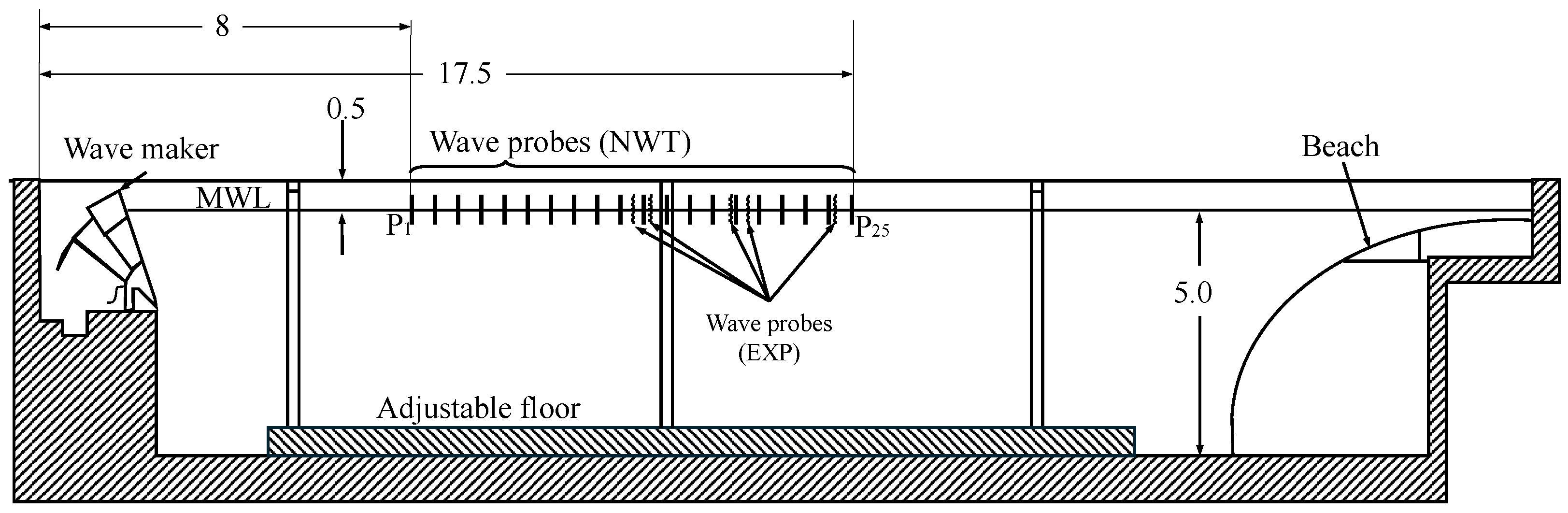
Accurate short-term wave forecasting is crucial for the active control of floating structures, with applications ranging from improving energy efficiency in wave energy converters to reducing wave-induced fatigue in floating wind turbine platforms. To achieve that, reliable upstream wave information must be available. The experimental campaign presented here was designed to emulate this requirement. Five wave probes were deployed with two closely spaced upstream closest to the wave maker, two downstream, and one located furthest downstream at the location of the floating wind turbine to be tested in later campaigns, as reported in Fowler [33] and Alkarem et al. [2]. The experiment took place at the Harold Alfond wind-wave (W2) basin at the Advanced Structures and Composites Center located at the University of Maine. A 1:70 Froude scaling was applied. The basin layout and probe distribution used for analysis are illustrated in Figure 1.
To complement the experimental study, The basin was numerically replicated using the higher-order spectral numerical wave tank (HOS-NWT) model developed by Bonnefoy et al. [27] and Ducrozet et al. [28], hereafter referred to as NWT. The simulated tank dimensions are 30 m in length, 10 m in width, and 5 m in depth. A wave absorbing beach is positioned at 85% of the tank length and configured with an absorption strength of 90%. In addition to the experimental probe configuration, additional virtual wave probes in the numerical wave tank were incorporated to enhance spatial resolution, resulting in a total of 25 probes distributed primarily at 0.5 m intervals.

2.2. Wave Forecasting Model Development

Two machine-learning-based models were investigated in this study. These models were trained using available data from either physical experiments (EXP) or the numerical wave tank (NWT) simulations. During testing, past data from all sensors were provided as input. The internal mapping learned during training is designed to correlate free surface elevations recorded by upstream probes with their subsequent propagation toward downstream locations. As a result, the models can forecast future wave elevations downstream based on historical probe measurements.
The first model is a recurrent neural network (RNN) of the multivariate long short-term memory (LSTM) type. LSTMs are well-regarded for their ability to retain both short- and long-term temporal dependencies with a forget gate to regulate the flow of past information, making them effective for time-series forecasting [34]. The second model is time-series dense encoder (TiDE), a state-of-the-art deep learning architecture proposed by Das et al. [35] designed to be more efficient and to potentially outperform more complex models. For time-series manipulation and model implementation, we used the open-source Python library Darts, developed by Unit8 SA [36].
Both models were trained using consistent hyperparameter settings: 1000 epochs, a batch size of 32, a hidden layer size of 100, a dropout rate of 0.1, and an optimizer learning rate of 0.001. A probabilistic forecasting framework was adopted through the use of the Laplace likelihood, which enables the models to produce a distribution of likely outcome to generate uncertainty bounds for each prediction. Performing uncertainty quantification (UQ) is crucial in the context of phase-resolved, ocean wave forecasting as it allows the systematic evaluation of confidence levels associated with each prediction. This is particularly useful when control systems are influenced by phase-resolved predictive models to reduce risks and high fatigue on these systems.
In both models, the same input–output structure was employed: a historical sequence of length, m is used to forecast a future horizon of n steps. A ratio of m / n = 2 is utilized. This implies that for a prediction horizon of τ = 1 s , the model observes two seconds of past data to predict one second ahead. The value of n was initially set to 120. With a temporal resolution of Δ t = 0.5 s , this corresponds to a forecasting horizon of τ = n × Δ t = 60 s . This selection was informed by the range of group velocities c g associated with the sea-state under consideration, given all numerical probes are active. We use group velocity since the energy content of the wave field propagates downstream with the group velocity, given in LWT by
c g = ω 2 k 1 + 2 k h sinh 2 k h ,
where ω and k denote the angular wave frequency and wavenumber, respectively, and h is the water depth. In sufficiently deep water conditions (i.e., k h > π ), the group velocity asymptotically approaches half the wave phase velocity, c = ω / k .
Since the multivariate forecasting problem is complex to define, we present here a uni-variate counterpart for simplicity. We create a forecast of the surface elevation target, y, given a known dynamic history of itself and other covariates, x, which can be written as
[ y i : i + n ] f [ y i m : i 1 ] , [ x i m : i 1 ] .
In the TiDE model, the upstream probes were considered as covariates (meant to help build the prediction, but their signal is not included in the forecast). However, the LSTM used all probes as variables. Due to causality, this would generate wrong forecasts at the most upstream probes, and the propagation of that error downstream is possible.
To quantify the error between the predicted variable, y, and the observed signal, y ^ , we calculated the mean absolute error (MAE) metric as
MAE = i = 1 n | y i y i ^ | n .
Two sea-states were being investigated in this research, a moderate one (SS1) and a severe one (SS2), both described by a JONSWAP spectrum using three parameters: the significant wave height, H s , peak wave period, T p , and the peak enhancement factor, γ . These parameters are detailed in Table 2.

2.3. Data Masking

We simulated two scenarios concerning the input data fed into the models. The first involves a temporal Monte Carlo dropout (or masking) of input signals from upstream buoys, representing either short- or long-term data loss. Short-term masking affects multiple sensors and occurs frequently in both space and time but only for short durations, Δ t m s k . This setup evaluates challenges such as intermittent signal acquisition—caused, for example, by low-visibility conditions affecting LIDAR—or shadowing effects. In contrast, long-term masking of a limited number of sensors tests the model’s resilience in maintaining predictive accuracy under conditions of sensor malfunction, power loss, or prolonged shadowing effects.
This methodology addresses a key challenge in data-driven modeling: handling highly irregular spatiotemporal input, such as LIDAR data, and converting it into a structured format suitable for models requiring uniform input. Figure 2 illustrates the adopted masking strategy used to simulate missing or corrupted input data via a Monte Carlo-style dropout mechanism. To implement this, time-series signals are first segmented into consecutive windows of size Δ t m s k . Each window is then assigned a random number drawn from a uniform distribution between 0 and 1. If the random number exceeds a predefined probability threshold ρ , the corresponding window is masked by multiplying the signal with a factor of zero, effectively simulating data loss. By adjusting ρ , one can control the frequency of dropout events throughout the signal. The figure presents two representative examples using different values of Δ t m s k : one with short-term masking and another with longer windows. The shorter windows result in more frequent dropout patterns, mimicking high-frequency signal interruptions. In contrast, the longer windows introduce more persistent, low-frequency masking, representing prolonged data outages. This dual-scale masking approach allows us to assess the model’s resilience to both transient and extended periods of data unavailability.
The second scenario introduces a phase shift to signals from upstream buoys. This simulates real-time data collection from floating wave sensors, which may drift and change position due to ocean currents and wave forces, resulting in positive or negative phase shifts in the recorded signals. Figure 3 shows an example of this effect. We assess model resilience to such phase discrepancies and quantify the corresponding degradation in predictive performance.

2.4. τ -Trimming Algorithm

Zhang et al. [20] used uncertainty-based parameterization to define a predictable zone for wave forecasting. In this study, we extended this approach to multivariate signal processing, incorporating uncertainty levels derived from historical forecasts.
First, we computed the uncertainty level for each target signal, y j ^ as follows:
δ ( y j ^ ) = q 0.975 ( y j ^ ) q 0.025 ( y j ^ ) ,
where q 0.975 and q 0.025 represent the 97.5th and 2.5th percentiles of the predicted distribution for y ^ j . We then defined a minimum uncertainty threshold,
δ 0 = 1 M j = 1 M δ min j + 0.25 ( δ max j δ min j ) ,
below which the forecast y j ^ was considered reliable, i.e., when δ ( y j ^ ) < δ 0 ; where M is the number of output signals, and δ min j and δ max j are the minimum and maximum observed uncertainties for each signal j.
Models that adapt their prediction horizon based on this threshold were referred to as τ -trimmed models, for which τ , the horizon, was computed as the time during which the uncertainty stays below δ 0 . For each historical forecast, this time horizon was computed by the following:
  • smoothing the uncertainty signal δ ( y ^ j ) using a 1D convolution with a Gaussian kernel,
  • finding the total time during which δ ( y ^ j ) < δ 0 , and
  • summing the number of valid time steps and multiplying by the time resolution Δ t to obtain τ .
Two types of τ -trimming algorithm were defined:
  • Moderate-type: for where τ was selected based on the peak of the distribution of valid horizons (or the average of all peaks in case of multivariate).
  • Conservative-type: which used the smallest τ that occurred in the distribution, beyond which the uncertainty threshold can be violated.
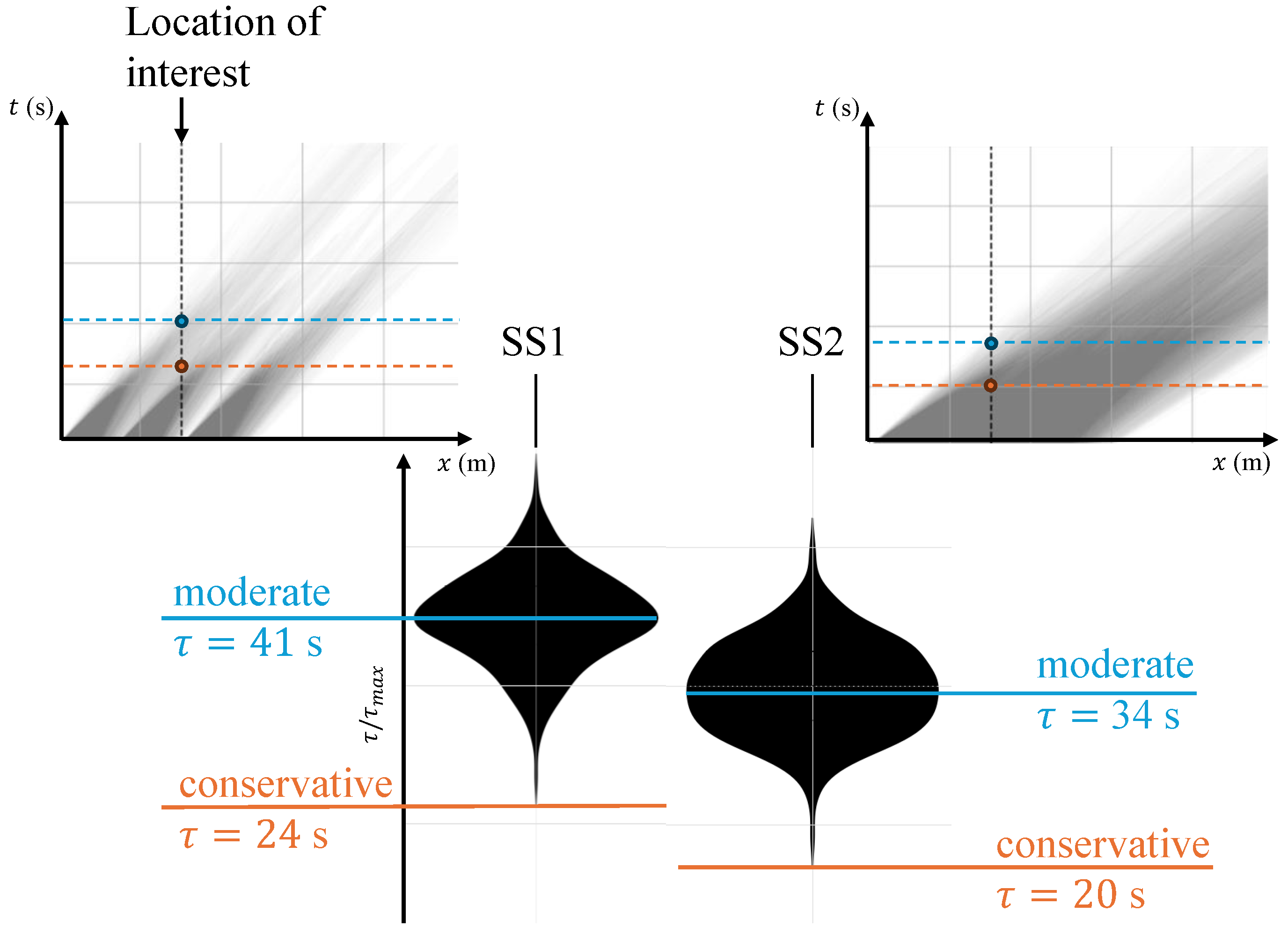
Figure 4a shows the resulting τ distribution (via violin plots) for the TiDE model applied to numerical wave tank data, focusing on the most downstream probes. Figure 4b illustrates a single forecast stride contributing to this distribution, highlighting how τ increases downstream as the model benefits from accumulating upstream information. This trend is also reflected in the violin plots.

3. Results

In the following, we present results of applying the machine learning models developed in this study to numerically and experimentally generated wave data and evaluate their performance and resilience under various input masking scenarios.

3.1. Numerical Wave Tank Investigation

Results of the HOS-NWT model provide highly resolved data at sensor (probe) locations, resulting in rich datasets that improve the predictive model learning and prediction accuracy. Only the moderate, SS1 sea-state was considered in this section (Table 2). We define the baseline model as the model that uses LWT to determine their prediction horizon regardless of uncertainty-related information generated by historical forecast. The prediction horizon of the baseline is defined by τ max , as illustrated in Figure 4. Then, we apply the τ -trimming algorithm as described in Section 2.4. The following tasks were conducted:
  • Benchmarking the baseline model performance against an uncertainty-based τ -trimming algorithm;
  • Evaluating the effects of short- and long-term input data masking on prediction accuracy;
  • Comparing a covariate-based model (TiDE) with a non-covariate-based model (LSTM).
To conduct a comprehensive sensitivity analysis, we defined four levels of masking probability thresholds, ρ = { 0 , 0.25 , 0.5 , 0.75 } . When ρ = 0 , no masking is applied—this represents the ideal case where all probes function correctly and no randomness or masking is introduced. In contrast, higher ρ values increase the likelihood of masking across time windows. Short- and long-term masking durations are defined by the window length Δ t m s k , as illustrated in Figure 2. Specifically, we selected a high-frequency, short-term masking window size of Δ t m s k = 25 s and a low-frequency, long-term masking window size of Δ t m s k = 250 s.
Figure 5 and Figure 6 show the performance of the LSTM and TiDE models, respectively, applied to numerically generated data. Each figure presents the performance MAE metric (Equation (3)) between observed and predicted values for the most downstream sensors. The top row of subplots corresponds to short-term data masking, while the bottom row corresponds to long-term masking. Within each row, the left subplot shows results for the baseline model, and the right subplot shows results for the corresponding model when the τ -trimming algorithm is activated. Overall, model performance deteriorates as the masking probability threshold increases as expected. The use of a τ -trimming algorithm effectively reduces the error and uncertainty bounds across the different probe locations (components). The results were analyzed in the form of comparing the baseline models to the trimmed ones, investigating short-term and long-term masking effects on performance, and comparing LSTM to TiDE models in the following sections.

3.1.1. Baseline and τ -Trimming Algorithm Comparison

A general trend can be observed when comparing the left and right subplots in Figure 5 and Figure 6: the τ -trimming algorithm consistently yielded lower MAE values compared to the baseline models. However, both model types converged to similarly low error levels as waves propagate downstream, suggesting a reduced benefit of applying the τ -trimming algorithm to later spatial positions.
Table 3 and Table 4 provide MAE values for probes p19 and p24 under short-term masking scenarios for the LSTM and TiDE models, respectively. In both tables, the last column reports the relative difference in MAE values between the baseline and τ -trimmed model. Negative values indicate that the τ -trimming algorithm outperforms the baseline model for the same wave data and masking scenario. The largest observed improvement occurred at probe p19 for ρ = 0 , where the τ -trimmed LSTM model achieved a 56% reduction in error. As ρ increased (more masking is applied to probes), this performance gap narrowed. This is expected, as both models are increasingly challenged by the loss of input data.

3.1.2. Impact of Short-Term vs. Long-Term Data Masking on Model Accuracy

Figure 5 and Figure 6 show the mean and 95% confidence intervals based on 10 repeated trials (a preliminary sensitivity analysis—not shown here—indicated that 10 repetitions were sufficient to produce representative results). The confidence intervals, visualized as transparent bands around the mean, were consistently wider for long-term masking scenarios compared to short-term ones, regardless of the model used. This indicates that extended data loss has a more detrimental and variable impact on forecasting accuracy than intermittent, shorter-term masking.

3.1.3. Comparison of the TiDE and LSTM Model Results

Both the TiDE and LSTM models performed well under the tested masking conditions. However, notable differences emerged in error variation spatially. Specifically, the TiDE model results exhibited a more pronounced error in upstream targets (e.g., p19), as seen in Figure 6a,c. In contrast, the LSTM model results showed relatively uniform error levels from upstream to downstream targets, as shown in Figure 5.
According to Table 4, TiDE model results had an error difference exceeding 50% between p19 and p24 when ρ = 0 , which decreased to 35% when ρ = 0.75 . LSTM model results, on the other hand, yielded a smaller difference of 34% for ρ = 0 , which narrowed substantially to only 3% for ρ = 0.75 (Table 3). This suggests that LSTM is more consistent across locations, while TiDE may be more sensitive to input data availability, especially for upstream targets.
It is worth noting that the LSTM was more computationally demanding and prone to casuality-related issues at upstream locations that could propagate downstream, affecting its resilience. However, LSTM models demonstrated on average lower error values than TiDE.

3.2. Experimental Investigation

In the following, we present the results of applying the machine learning models to experimental data acquired in the University of Maine basin. While the numerical investigation demonstrated the models’ ability to forecast downstream free surface elevations with high spatial resolution, it is equally important to assess model performance under more constrained conditions—specifically, when data are only available on a coarser spatial grid of sensors/probes, and additional input masking is applied.
Data acquired from experiments run for both sea-states SS1 and SS2, described in Table 2, were considered in this analysis. Two variants of the TiDE model were developed to explore differences in the predictable zone. The first follows the moderate-type strategy used in the numerical study, while the second adopted a more conservative approach, deemed necessary due to the reduced number of upstream probes. These two variants are illustrated schematically in Figure 7.
For the moderate-type model, the dynamic prediction horizons were computed as τ = 41 s for SS1 and 34 s for SS2. The conservative-type model used shorter horizons of τ = 24 s and 20 s, respectively. When overlaid as horizontal dashed lines on the space–time (upper) plots of Figure 7, these τ values aligned well with the predictable zone shadows inferred from the upstream probes (using LWT group velocities). Specifically, the moderate horizon coincided with the predictable zones generated by the first and second probes, while the conservative horizon aligned with zones generated by the third and fourth probes—those closest to the target location. This alignment suggests that relying on more distant upstream data may introduce higher uncertainty due to wave dispersion effects, as waves travel downstream.
The group-velocity-based predictable zone shadows shown in Figure 7 (upper space–time plots) were computed using the minimum and maximum group velocities with Equation (1), applied over a 50-second moving window. It is also worth noting that waves in SS2 propagate faster (as they are longer-period), which naturally results in shorter prediction horizons for both model types.

Sensitivity to Data Availability Under Spatially Coarse Grid Constraint

As in the previous section, we assessed the models’ performance under both short- and long-term data masking scenarios. Here, we set the masking probability threshold to ρ = 0.25 and varied only the masking duration. Figure 8 presents the resulting error levels for both the moderate- and conservative-type prediction horizons. The error bars represent the 95% confidence intervals.
Figure 8a shows that the overall MAE levels remain relatively high, yet comparable to those from the NWT-based analysis. This indicates that the models were still capable of delivering phase-resolved wave forecasts even when operating under coarser spatial resolution—i.e., with fewer upstream probes.
To further illustrate the effect of long-term data loss on wave forecast accuracy, Figure 9 shows the instantaneous MAE between the original signal and the model’s historical forecast, along with a smoothed MAE error curve, using a Gaussian filter. Two scenarios are presented: (1) under healthy operating conditions where all covariates were active and (2) when a single covariate (the third upstream probe) went offline. The results clearly show increased error spikes and a higher smoothed error level when the covariate was unavailable, highlighting the importance of upstream sensor reliability.

3.3. Phase Shift Effects of Upstream Data

To simulate the effects of drifting ocean sensors, a phase shift mask was applied to the signals from the first and second experimental wave probes (out of five). A sensitivity analysis was then performed by varying the introduced phase shift, θ , to evaluate its impact on wave forecast accuracy for both the moderate- and conservative-type models.
Note that the magnitude of the phase shift corresponds to the physical displacement of the buoy within its watch circle governed by the sea-state. For example, the wave celerity (i.e., phase velocity) of SS1 is approximately 14 m/s at the peak period. Thus, a 1-s phase shift implies a horizontal displacement of about 14 m, assuming frozen-phase wave propagation. Given realistic mooring constraints, high phase shifts are unlikely for properly moored buoys. Nevertheless, to evaluate model resilience, we swept θ values across a broad range, from 10 to + 10 s.
Thus, Figure 10 shows how the MAE varies as a function of phase shift, θ , applied to the first two upstream probes. The results indicated a substantial sensitivity of the MAE to phase perturbations, especially for the moderate-type model. The conservative model maintained lower error levels overall.

4. Discussion

The numerical investigation of wave forecasting errors using the various models demonstrated that when sufficient upstream data are available, the machine learning models are capable of accurately forecasting phase-resolved ocean waves, even in the presence of data loss. However, the role of uncertainty quantification is critical: without constraining prediction uncertainty, errors can exceed acceptable thresholds, potentially jeopardizing the reliability of downstream applications, such as wave-aware control systems.
The results showed that long-term data masking leads to significantly wider uncertainty bounds compared to short-term masking. This indicates that prolonged data loss introduces higher variability in model outputs. The use of a τ -trimming algorithm mitigates this effect, maintaining lower error levels by adjusting the prediction horizon based on previous forecast uncertainty levels.
Although the LSTM model exhibited lower average error values (Figure 5), it also suffered from causality-related issues. Specifically, erroneous predictions at the most upstream probes can propagate downstream if intermediate probes do not provide sufficient supplementary information. Moreover, LSTM models require longer training times due to the need to forecast multiple targets simultaneously. TiDE models, in contrast, provide a good balance between accuracy and computational cost, as was also pointed out by Harris [29].
TiDE models showed strong performance under densely spaced upstream probes. However, under experimental conditions with coarser spatial probe resolution and more energetic sea-states, the moderate-type model exhibited a degraded accuracy. To address this, we introduced a conservative-type τ -trimming algorithm with shorter prediction horizons, derived from uncertainty thresholds. This version demonstrated greater resilience to both data loss and phase shifts. For instance, MAE was reduced by 30% when the conservative variation was used during short and long-term masking, as seen in Figure 8. Additionally, an increase in MAE by about 0.5 m was observed with a deviation of ±3 s from the optimal phase alignment. The same error accumulated when using the conservative approach at ±4 s.
The phase shift analysis reveals that drifting upstream probes can degrade the wave forecast accuracy downstream, more severely than complete data masking. This insight suggests the potential value of dynamically deactivating unreliable sensors in real time, rather than feeding uncertain signals into the models. Moreover, for data acquisition systems with irregular spatial or temporal coverage—such as LIDAR—the model should be trained assuming a maximum upstream sensor grid. Irregularities can then be handled via dynamic masking to reflect real-time sensor availability based on acquired data locations.
Despite the promising results, several limitations of this study must be acknowledged. The models were trained and tested under fixed sea-state conditions (specific H s and T p ) and are not generalizable across varying sea states without retraining. In real-time applications, a classifier would be required to identify the prevailing sea state and activate the corresponding trained model. Additionally, the dynamic behavior of drifting buoys was not explicitly modeled. Instead, sensor drift was approximated by applying phase shifts to fixed probes. This simplification neglects wave transient changes due to wave dispersion, as well as the impact of buoy motion on measurement accuracy.
Building upon these findings, future work will explore the following directions. The τ -trimming algorithm can be further enhanced by including performance-guided limitations instead of purely uncertainty-based. This involves dynamically adjusting the forecast horizon to ensure error remains below a threshold determined from weighted historical forecast performance. The authors are also interested in extending the methodology to real ocean field deployments where wave conditions include short-crested, multi-directional, and wave–current interaction effects. This will allow for validation in more complex and nonlinear environments. Furthermore, wave forecasting model can be integrated with floating platform simulations to predict wave-induced loads and platform responses in real time, enabling more effective digital twin and control applications.
Overall, these results support the development of flexible, uncertainty-aware forecasting models that are resilient to realistic operational challenges such as missing data, probe drift, and coarse spatial resolution in offshore wave monitoring systems and control strategies.

5. Conclusions

This study evaluated the performance and resilience of ML models for phase-resolved ocean wave forecasting under conditions of incomplete and uncertain upstream data flow. Using both numerical wave tank simulations and experimental datasets, we tested two ML models; LSTM and TiDE, across scenarios involving data masking, phase shifts, and spatial sparsity of upstream probes. We demonstrated that the τ -trimming algorithm that limits the prediction horizon based on uncertainty levels effectively reduces wave forecasting errors by 46% for the TiDE model and 22% for the LSTM model with a masking probability threshold of ρ = 0.5 .
While LSTM models showed lower average errors, they were more computationally demanding and prone to causality-related inaccuracies at upstream locations. The TiDE model, especially in its conservative τ -trimmed form, offered a more resilient alternative under experimental constraints, including probe drift and reduced sensor availability. For instance, a reduction of 30% in forecast error was observed under short and long-term masking.
These findings reinforce the importance of incorporating uncertainty quantification and phase-awareness into ML-based forecasting frameworks for offshore applications. In practice, many ocean measurement systems operate in dynamic and uncertain environments where upstream data availability is inconsistent. The τ -trimming method offers a practical mechanism to regulate forecast reliability in real time without requiring model retraining or structural modifications.
While this study demonstrates the viability of τ -trimmed forecasting under sparse and uncertain data conditions, several limitations remain. The models were trained for specific sea states and do not generalize across varying conditions without retraining or classification-based switching. Additionally, drifting probe effects were simplified as static phase shifts, omitting dynamic amplitude and dispersion-related changes that occur in real deployments. Future work will address these limitations by extending the method to real ocean field data with multidirectional and nonlinear wave effects and by integrating forecasting with floating structure response models. An adaptive, performance-guided version of τ -trimming will also be explored to maintain target error thresholds in real time.

Author Contributions

Conceptualization, Y.R.A.; data curation, Y.R.A.; formal analysis, Y.R.A.; funding acquisition, K.H., R.W.K. and S.T.G.; investigation, Y.R.A. and S.T.G.; methodology, Y.R.A.; project administration, K.H., R.W.K. and S.T.G.; resources, K.H. and R.W.K.; software, Y.R.A.; supervision, K.H., R.W.K. and S.T.G.; validation, S.T.G.; visualization, Y.R.A.; writing—original draft, Y.R.A. and S.T.G.; writing—review and editing, Y.R.A., K.H., R.W.K. and S.T.G. All authors have read and agreed to the published version of the manuscript.

Funding

The authors gratefully acknowledge funding from the US Department of Energy-Office of Science, under grants #: DE-SC0022103 and # DE-SC0024295 (DOE-EPSCOR program), awarded to the University of Rhode Island and the University of Maine.

Data Availability Statement

The data supporting the findings of this study are available in the DOLPHINN GitHub repository (development branch) at https://github.com/Yuksel-Rudy/DOLPHINN/tree/dev.

Conflicts of Interest

The authors declare no conflicts of interest.

References

  1. Li, G.; Weiss, G.; Mueller, M.; Townley, S.; Belmont, M.R. Wave energy converter control by wave prediction and dynamic programming. Renew. Energy 2012, 48, 392–403. [Google Scholar] [CrossRef]
  2. Alkarem, Y.R.; Huguenard, K.; Kimball, R.W.; Hejrati, B.; Ammerman, I.; Nejad, A.R.; Grilli, S. On Building Predictive Digital Twin Incorporating Wave Predicting Capabilities: Case Study on UMaine Experimental Campaign-FOCAL. In Journal of Physics: Conference Series; IOP Publishing: Bristol, UK, 2024; Volume 2745, p. 012001. [Google Scholar]
  3. Albertson, S.T.; Gharankhanlou, M.; Steele, S.C.; Grilli, S.T.; Dahl, J.M.; Grilli, A.R.; Huguenard, K. Improved control of floating offshore wind turbine motion by using phase-resolved wave reconstruction and forecast. In Proceedings of the ISOPE International Ocean and Polar Engineering Conference, ISOPE, Ottawa, ON, Canada, 19–23 June 2023; p. ISOPE–I. [Google Scholar]
  4. Flotco. Flotco Technology. 2024. Available online: https://www.flotco.tech (accessed on 15 May 2025).
  5. Korniejenko, K.; Gądek, S.; Dynowski, P.; Tran, D.H.; Rudziewicz, M.; Pose, S.; Grab, T. Additive Manufacturing in Underwater Applications. Appl. Sci. 2024, 14, 1346. [Google Scholar] [CrossRef]
  6. Grilli, S.T.; Guérin, C.A.; Goldstein, B. Ocean wave reconstruction algorithms based on spatio-temporal data acquired by a flash LiDAR camera. In Proceedings of the ISOPE International Ocean and Polar Engineering Conference, ISOPE, Maui, HI, USA, 19–24 June 2011; p. ISOPE–I. [Google Scholar]
  7. Morris, E.; Zienkiewicz, H.; Belmont, M. Short term forecasting of the sea surface shape. Int. Shipbuild. Prog. 1998, 45, 383–400. [Google Scholar]
  8. Desmars, N.; Bonnefoy, F.; Grilli, S.T.; Ducrozet, G.; Perignon, Y.; Guérin, C.A.; Ferrant, P. Experimental and numerical assessment of deterministic nonlinear ocean waves prediction algorithms using non-uniformly sampled wave gauges. Ocean Eng. 2020, 212, 107659. [Google Scholar] [CrossRef]
  9. Naaijen, P.; Huijsmans, R. Real time wave forecasting for real time ship motion predictions. In Proceedings of the International Conference on Offshore Mechanics and Arctic Engineering, Estoril, Portugal, 15–20 June 2008; Volume 48210, pp. 607–614. [Google Scholar]
  10. Wu, G. Direct Simulation and Deterministic Prediction of Large-Scale Nonlinear Ocean Wave-Field. Ph.D. Thesis, Massachusetts Institute of Technology, Cambridge, MA, USA, 2004. [Google Scholar]
  11. Qi, Y.; Wu, G.; Liu, Y.; Yue, D.K. Predictable zone for phase-resolved reconstruction and forecast of irregular waves. Wave Motion 2018, 77, 195–213. [Google Scholar] [CrossRef]
  12. Nouguier, F.; Guérin, C.A.; Chapron, B. “Choppy wave” model for nonlinear gravity waves. J. Geophys. Res. Ocean. 2009, 114. [Google Scholar] [CrossRef]
  13. Nouguier, F.; Grilli, S.T.; Guérin, C.A. Nonlinear ocean wave reconstruction algorithms based on simulated spatiotemporal data acquired by a flash LIDAR camera. IEEE Trans. Geosci. Remote Sens. 2013, 52, 1761–1771. [Google Scholar] [CrossRef]
  14. Guérin, C.A.; Desmars, N.; Grilli, S.T.; Ducrozet, G.; Perignon, Y.; Ferrant, P. An improved Lagrangian model for the time evolution of nonlinear surface waves. J. Fluid Mech. 2019, 876, 527–552. [Google Scholar] [CrossRef]
  15. Kim, I.C.; Ducrozet, G.; Bonnefoy, F.; Leroy, V.; Perignon, Y. Real-time phase-resolved ocean wave prediction in directional wave fields: Enhanced algorithm and experimental validation. Ocean Eng. 2023, 276, 114212. [Google Scholar] [CrossRef]
  16. Wijaya, A.; Naaijen, P.; Van Groesen, E. Reconstruction and future prediction of the sea surface from radar observations. Ocean Eng. 2015, 106, 261–270. [Google Scholar] [CrossRef]
  17. Al-Ani, M.; Belmont, M.; Christmas, J. Sea trial on deterministic sea waves prediction using wave-profiling radar. Ocean Eng. 2020, 207, 107297. [Google Scholar] [CrossRef]
  18. Mohaghegh, F.; Murthy, J.; Alam, M.R. Rapid phase-resolved prediction of nonlinear dispersive waves using machine learning. Appl. Ocean Res. 2021, 117, 102920. [Google Scholar] [CrossRef]
  19. Wang, N.; Chen, Q.; Chen, Z. Reconstruction of nearshore wave fields based on physics-informed neural networks. Coast. Eng. 2022, 176, 104167. [Google Scholar] [CrossRef]
  20. Zhang, J.; Zhao, X.; Jin, S.; Greaves, D. Phase-resolved real-time ocean wave prediction with quantified uncertainty based on variational Bayesian machine learning. Appl. Energy 2022, 324, 119711. [Google Scholar] [CrossRef]
  21. Jörges, C.; Berkenbrink, C.; Stumpe, B. Prediction and reconstruction of ocean wave heights based on bathymetric data using LSTM neural networks. Ocean Eng. 2021, 232, 109046. [Google Scholar] [CrossRef]
  22. Kagemoto, H. Forecasting a water-surface wave train with artificial intelligence—A case study. Ocean Eng. 2020, 207, 107380. [Google Scholar] [CrossRef]
  23. Duan, W.; Ma, X.; Huang, L.; Liu, Y.; Duan, S. Phase-resolved wave prediction model for long-crest waves based on machine learning. Comput. Methods Appl. Mech. Eng. 2020, 372, 113350. [Google Scholar] [CrossRef]
  24. Silva, K.M.; Maki, K.J. Data-Driven system identification of 6-DoF ship motion in waves with neural networks. Appl. Ocean Res. 2022, 125, 103222. [Google Scholar] [CrossRef]
  25. Gal, Y.; Ghahramani, Z. A theoretically grounded application of dropout in recurrent neural networks. Adv. Neural Inf. Process. Syst. 2016, 29, 1027–1035. [Google Scholar]
  26. Law, Y.; Santo, H.; Lim, K.; Chan, E. Deterministic wave prediction for unidirectional sea-states in real-time using Artificial Neural Network. Ocean Eng. 2020, 195, 106722. [Google Scholar] [CrossRef]
  27. Bonnefoy, F.; Ducrozet, G.; Le Touzé, D.; Ferrant, P. Time domain simulation of nonlinear water waves using spectral methods. In Advances in Numerical Simulation of Nonlinear Water Waves; World Scientific: Singapore, 2010; pp. 129–164. [Google Scholar]
  28. Ducrozet, G.; Bonnefoy, F.; Le Touzé, D.; Ferrant, P. A modified high-order spectral method for wavemaker modeling in a numerical wave tank. Eur. J. Mech.-B/Fluids 2012, 34, 19–34. [Google Scholar] [CrossRef]
  29. Harris, J.C. Faster than real-time, phase-resolving, data-driven model of wave propagation and wave–structure interaction. Appl. Ocean Res. 2025, 154, 104291. [Google Scholar] [CrossRef]
  30. Li, R.; Zhang, J.; Zhao, X.; Wang, D.; Hann, M.; Greaves, D. Phase-resolved real-time forecasting of three-dimensional ocean waves via machine learning and wave tank experiments. Appl. Energy 2023, 348, 121529. [Google Scholar] [CrossRef]
  31. Ma, X.; Huang, L.; Duan, W.; Li, P.; Wang, Z. Experimental investigations on the predictable temporal-spatial zone for the deterministic sea wave prediction of long-crested waves. J. Mar. Sci. Technol. 2022, 27, 252–265. [Google Scholar] [CrossRef]
  32. Qi, Y.; Wu, G.; Liu, Y.; Kim, M.H.; Yue, D.K. Nonlinear phase-resolved reconstruction of irregular water waves. J. Fluid Mech. 2018, 838, 544–572. [Google Scholar] [CrossRef]
  33. Fowler, M.J.L. Floating Offshore-Wind and Controls Advanced Laboratory Program: 1: 70-Scale Testing of a 15 Mw Floating Wind Turbine; The University of Maine: Orono, ME, USA, 2023. [Google Scholar]
  34. Hochreiter, S.; Schmidhuber, J. Long short-term memory. Neural Comput. 1997, 9, 1735–1780. [Google Scholar] [CrossRef]
  35. Das, A.; Kong, W.; Leach, A.; Mathur, S.; Sen, R.; Yu, R. Long-term forecasting with tide: Time-series dense encoder. arXiv 2023, arXiv:2304.08424. [Google Scholar]
  36. Darts: User-Friendly Forecasting in Python. 2021. Available online: https://github.com/unit8co/darts (accessed on 30 May 2025).
Figure 1. Vertical cross-section of the Harold Alfond wind-wave (W2) basin, located at the Advanced Structures and Composites center (modified from Fowler [33]). Units are in meter. This basin was numerically replicated in the HOS-NWT model.
Jmse 13 01250 g001
Figure 2. Short- and long-term data masking to simulate a Monte Carlo dropout of input signals.
Jmse 13 01250 g002
Figure 3. Phase shift to simulate drift-induced phase changes in floating wave sensor data.
Jmse 13 01250 g003
Figure 4. Development of τ -trimming algorithm using uncertainty quantification: (a) Normalized prediction horizon distribution of τ -trimmed TiDE model for multivariate target, using NWT data. (b) A single stride historical forecast example with uncertainty level curves and their smoothed versions. The vertical dashed lines show τ trimmed values when uncertainty levels peak over δ 0 mean threshold.
Jmse 13 01250 g004
Figure 5. Prediction error using LSTM models with NWT data for four probability thresholds ρ = { 0 , 0.25 , 0.5 , 0.75 } . (a) Baseline model under short-term masking. (b) τ -trimming algorithm under short-term masking. (c) Baseline model under long-term masking. (d) τ -trimming algorithm under long-term masking.
Jmse 13 01250 g005
Figure 6. Prediction error using TiDE models with NWT data for four probability thresholds ρ = { 0 , 0.25 , 0.5 , 0.75 } . (a) Baseline model under short-term masking. (b) τ -trimming algorithm under short-term masking. (c) Baseline model under long-term masking. (d) τ -trimming algorithm under long-term masking.
Jmse 13 01250 g006
Figure 7. Normalized prediction horizon distribution of τ -trimming algorithm under two sea-state conditions, for experimental data. Horizontal dashed lines represent τ values for the moderate-type and conservative-type models for each sea-state, superimposed on LWT-based predictable zone shadows. These shadows are computed from minimum and maximum group velocities using upstream probe locations.
Jmse 13 01250 g007
Figure 8. Impact of short- and long-term data masking on model performance, for experimental data: (a) MAE for moderate and conservative prediction horizons under sea-state SS1. (b) MAE for moderate and conservative prediction horizons under sea-state SS2.
Jmse 13 01250 g008
Figure 9. Instantaneous and smoothed MAE error over time under two conditions for experimental data: (i) healthy operations with all covariates active and (ii) loss of the third covariate probe.
Jmse 13 01250 g009
Figure 10. Impact of phase shift θ , applied to the first two upstream probes, on model prediction accuracy under experimental conditions: (a) MAE for moderate and conservative prediction horizons under sea-state SS1. (b) MAE for moderate and conservative prediction horizons under sea-state SS2.
Jmse 13 01250 g010
Table 1. Comparison of research methods across previous studies and the current work.
Research MethodsPrevious StudiesThis Work
Numerical data generation[6,11,18,22,23,24]High-order spectral simulations using HOS-NWT
Experimental data generation[8,15,29,30]1:70 scale experiments using 5 wave probes at the W2 wave basin
Physics-based modeling[6,8,12,13]Used for baseline horizon estimation
Data-driven modeling[15,18,22,23,24,29,30]Implemented using LSTM and TiDE for wave prediction
Moving probes[11] (analytical only), [32]Sensitivity analysis via phase shift scenarios with moving probes
Uncertainty quantification[20,24]Introduced τ -trimming algorithm for uncertainty-guided prediction horizon
Sensitivity to data scarcityNot explicitly addressedSystematic masking of upstream probe data with performance analysis
Table 2. Parameters of two sea-state being investigated.
ParametersSS1SS2
H s (m)3.2710.58
T p (s)9.0214.04
γ (-)1.82.75
Table 3. Comparison of MAE (m) for baseline and τ -trimmed LSTM model across different ρ values for probes p19 and p24 (short-term masking), for SS1-related wave data.
Probe ρ Baseline τ -TrimmedDiff.
p1900.1810.080−56%
0.250.2910.217−25%
0.50.4460.350−22%
0.750.5300.511−4%
p2400.1190.092−23%
0.250.2420.216−11%
0.50.4020.344−14%
0.750.5130.505−1%
diff.0−34%15%
0.25−17%−1%
0.5−10%−2%
0.75−3%−1%
Table 4. Comparison of MAE (m) for baseline and τ -trimmed TiDE model across different ρ values for probes p19 and p24 (short-term masking), for SS1-related wave data.
Probe ρ Baseline τ -TrimmedDiff.
p1900.1820.088−52%
0.250.8280.417−50%
0.51.0120.548−46%
0.750.9760.602−38%
p2400.0800.078−2%
0.250.4180.301−28%
0.50.5460.429−22%
0.750.6400.542−15%
diff.0−56%−12%
0.25−50%−28%
0.5−46%−22%
0.75−34%−10%
Disclaimer/Publisher’s Note: The statements, opinions and data contained in all publications are solely those of the individual author(s) and contributor(s) and not of MDPI and/or the editor(s). MDPI and/or the editor(s) disclaim responsibility for any injury to people or property resulting from any ideas, methods, instructions or products referred to in the content.

