Article

Assessing Coastal Degradation Through Spatiotemporal Earth Observation Data Cubes Analytics and Multidimensional Visualization

by
Ioannis Kavouras
*,†,
Ioannis Rallis
,
Nikolaos Bakalos
and
Anastasios Doulamis
School of Rural, Surveying and Geoinformatics Engineering, National Technical University of Athens, Zografou Campus 9, Iroon Polytechniou Str., 157 72 Attica, Greece
*
Author to whom correspondence should be addressed.
These authors contributed equally to this work.
J. Mar. Sci. Eng. 2025, 13(7), 1239; https://doi.org/10.3390/jmse13071239 (registering DOI)
Submission received: 3 June 2025 / Revised: 22 June 2025 / Accepted: 24 June 2025 / Published: 27 June 2025
(This article belongs to the Section Ocean Engineering)

Abstract

Coastal and maritime regions and their entities face accelerated degradation due to the combined effects of environmental stressors and anthropogenic activities. Coastal degradation can be identified, visualized and estimated through periodic monitoring over a region of interest using earth observation, climate, meteorological, seasonal, waves, sea level rising, and other ocean- and maritime-related datasets. Usually, these datasets are provided through different sources, in different structures or data types; in many cases, a complete dataset can be large in size and needs some kind of preprocessing (information filtering) before use in the intended application. Recently, the term data cube introduced in the scientific community and frameworks like Google Earth Engine and Open Data Cubes have emerged as a solution to earth observation data harmonization, federation, and exchange framework; however, these sources either completely lack the ability to process climate, meteorological, waves, sea lever rising, etc., data from open sources, like CORDEX and WCRP, or preprocessing is required. This study describes and utilizes the Ocean-DC framework for modular earth observation and other data types to resolve major big data challenges. Compared to the already existing approaches, the Ocean-DC framework harmonizes several types of data and generates ready-to-use data cubes products, which can be merged together to produce high-dimensionality visualization products. To prove the efficiency of the Ocean-DC framework, a case study at Crete Island, emphasizing the Port of Heraklion, demonstrates the practical utility by revealing degradation trends via time-series analysis of several related remote sensing indices calculated using the Ocean-DC framework. The results show a significant reduction in processing time (up to 89%) compared to traditional remote sensing approaches and optimized data storage management, proving its value as a scalable solution for environmental resilience, highlighting its potential use in early warning systems and decision support systems for sustainable coastal infrastructure management.

1. Introduction

Coastal regions, encompassing shorelines, maritime zones, and the port infrastructure, are subjected to severe environmental conditions that significantly accelerate material degradation. Prolonged exposure to climate conditions [1] like temperature fluctuations, high humidity, saltwater spray, precipitation, wave action, tidal forces, and wind speed drives multiple deterioration mechanisms, including metal corrosion, material erosion (affecting both natural landscapes and engineered structures such as concrete), and structural wear due to aging [2]. Furthermore, anthropogenic factors [3] such as oil exploitation [4], urbanization and tourism [5] exacerbate degradation, compounding the environmental stressors on these vulnerable ecosystems.
Coastal regions support a diverse range of human activities, from heavy industrial operations in port zones to recreational, scientific, and athletic pursuits (i.e., blue economy [6]). These areas are vital to societal wellbeing, influencing the economic, environmental, and public health dimensions [7]. Ensuring the sustainability of these activities requires safeguarding coastal zones against anthropogenic, environmental, and climate-induced degradation. Advanced analytics-driven early warning and decision support systems offer a robust approach to mitigating such deterioration, enhancing resilience in these critical ecosystems [8].
Modern monitoring systems benefit from vast and diverse datasets, typically generated from multiple sources with high volume and storage demands [9]. These data are often distributed across heterogeneous architectures, posing significant Big Data challenges [10]. To address these issues, raw datasets can undergo harmonization and homogenization processes. Furthermore, storing data in a structured and accessible manner facilitates efficient post-processing and enables multidimensional parameter visualization. Such an approach enhances the effectiveness of periodic coastal monitoring, supporting informed decision-making and long-term resilience.
This work introduces the OCEANIDS Data Cubes (Ocean-DC) framework as a tool for EO (Earth Observation) data harmonization, federation and homogenization. In particular, this work examines the efficiency of processing raw EO data, focusing mainly on Sentinel-2 and Landsat-8/9 missions, and generating ready-to-use multidimensional data cubes. By default, the Ocean-DC framework can be used for generating 3D products; however, by defining a time window frame, these data cubes products can be stored as 4D data cubes (hypercubes) either locally (i.e., on the end-users machine) or in online databases (i.e., on a data providers machine), which can be later used for coastal region monitoring based on time-series analysis. For better visualization, the final data cubes products are combined with additional information (i.e., Digital Elevation Models) to expand further their dimensionality.
In comparison with similar frameworks (i.e., Google Earth Engine [11] and Open Data Cubes [12]), the Ocean-DC framework is straightforward and tailored for coastal and maritime monitoring use cases and provides data that supports high-dimensional expansion. Unlike Google Earth Engine, which is only online based, the Ocean-DC framework can be installed anywhere and is supported by all major operating systems. In addition, the source code follows free and open standards, allowing the scientific community to build a demanding application upon it. Compared to Open Data Cubes, the Ocean-DC framework follows a similar approach but additionally supports climate/meteorological data, including waves and sea level datasets from CORDEX [13] repositories.
To prove the efficiency and effectiveness of the Ocean-DC data cubes, this manuscript presents a case study example. The case study uses monthly captured Sentinel-2 and Landsat-8/9 products of past years as raw data and generates EO Data Cubes using the Ocean-DC framework. As an area of interest, the island of Crete (Greece, Mediterranean) is selected, with emphasis on the port of Heraklion, which serves significant trade routes connecting Greece to various destinations across the Mediterranean and beyond. The research provide significant results and indicates the importance of utilizing traditional remote sensing approaches with innovative techniques for assessing coastal surface degradation through spatiotemporal analytics.
In summary, the contribution of this work is as follows:
  • This work introduces the Ocean-DC tool as an approach of EO data harmonization and homogenization.
  • This work addresses current Big Data challenges through the Ocean-DC tool implementation.
  • The Ocean-DC products provide a robust architecture for EO data management (i.e., storage, processing, and distribution).
  • Through the case study, we investigate the use of advance analytics tools for monitoring coastal degradation.
  • This work investigates the visualization of EO data in high-dimensional data structures.
The rest of the paper is structured as follows: (a) Section 2 provides related works of the current literature; (b) Section 3 describes the Ocean-DC tool; (c) Section 4 demonstrates the Ocean-DC tool and presents the results of the case study; (d) Section 5 discusses further the experimental results; and (e) Section 6 concludes this work.

2. Related Works

A data cube is defined as a multidimensional array or data structure that enables the efficient analysis of complex datasets across multiple dimensions. DC frameworks leverage this capability for big data storage and analytical processing [14], frequently involving complex queries [15] for data retrieval and analysis [16]. Key functionalities of DC frameworks include (a) multidimensional representation [17]; (b) cube-based visualization of big data [18]; (c) data aggregation [19]; (d) optimized query performance [20]; (e) OLAP operations [21]; and (f) smart big data applications [22].
In geosciences and especially in remote sensing and geospatial application, DC frameworks have become instrumental for data federation and harmonization. For example, ref. [23] implemented an Open Data Cube platform to generate Earth observation data cubes across Brazil, facilitating land use mapping through satellite imagery and temporal analysis. Similarly, ref. [24] evaluated the capabilities of Swiss DCs for monitoring snow cover dynamics in Gran Paradiso National Park using the Swiss Data Cube platform [25], an open-source solution designed for managing and analyzing large-scale Earth observation datasets.
Giuliani et al. [19,26] developed a methodological approach for land degradation assessment using Swiss DCs, incorporating solar geometry indicators to evaluate land productivity, soil organic carbon dynamics, and degradation patterns. Their work also introduced an automated "Data Cube on Demand" system that generates customized DCs based on user-specified parameters including geographic extent, sensor characteristics, and satellite product types.
The Australian Geoscience Data Cube [27] addresses fundamental Big Data challenges, volume, velocity and variety, enhancing Earth observation applications in water resource monitoring, coastal processes, agricultural assessment, forest cover change, and biodiversity studies. The work of Temenos et al. provides an example of recent innovations in context-aware adaptive DC framework for environmental monitoring and climate change mitigation.
Lastly, the Ocean-DC prototype was introduced in the previous work of Kavouras et al. [28]. The Ocean-DC prototype framework is designed for coastal and maritime monitoring near port infrastructures. In previous case study, the analysis was restricted to monitoring a close temporal window over the Piraeus region, emphasizing the oil spill accident in Saronic Gulf on the 10th of September 2017. Following the results of previous research, in this paper’s case study, they investigated the efficiency of the Ocean-DC tools and products for both EO products’ management and periodic coastal region monitoring, emphasizing the indication of coastal degradation patterns.

3. Proposed Methodology

The Ocean-DC framework was first introduced as a prototype implementation in our previous work [28]. Figure 1 illustrates the architecture of the current version of the Ocean-DC framework. The Ocean-DC architecture is designed to handle several kinds of data, both EO and non-EO, from different sources. This feature is not observed in existing frameworks like Google Earth Engine and Open Data Cubes, which are limited to EO data handling. The data collection is followed by the data harmonization process, which includes the core processes for generating the Ocean-DC products and exporting them as standardized NetCDF file formats. These products can be stored easily and processed in the same machine or stored in a server for sFTP or Geoserver for WMS/WFS data exchange. The final products can be used easily with traditional mapping techniques to produce multidimensional visualization models.
The Ocean-DC framework is designed under the EU Commission funded OCEANIDS project [29] for harmonizing, federate, and exchange data from different sources for monitoring coastline and maritime activities and degradation. According to the European Commission [30], there are several variables that could be useful to coastal erosion monitoring. The Ocean-DC framework’s architecture supports data corresponding to the following parameters:
  • Extreme wind speeds and waves: These data can be collected from climate or meteorological models (i.e., CORDEX mission [13]) or in situ data collection using local station (i.e., usually from national observatories).
  • Sea level: These data can be expressed as seasonal or annual variability, considering the local tectonics, subsidence, or uplifting of the coast. Tidal trends are also included in these data category. The World Climate Research Program (WCRP) [31] can be a source for such data.
  • Climate/Meteorological variables: The data can include climate/meteorological phenomena, variables and parameters such as temperature, humidity, precipitation, barometric forcing, etc. These data are mostly provided by models [13]. However, some of these parameters, such as temperature, can be collected, calculated or provided in EO data (i.e., TIRS bands in Landsat-8/9).
  • Coastal geology: Coastal geology can be monitored using the SWIR [32] bands of EO data (i.e., Landsat-8/9 and Sentinel-2) or geological maps.
  • Very high resolution bathymetry data: Such data can be downloaded from GEBCO [33]. The current version of the Ocean-DC framework does not process these data; however, they can be used raw, combined with Ocean-DC products for visualization enhancement.
  • Vegetation in the coastal zone: By calculating the NDVI or NDWI EO products, it is possible to monitor coastal vegetation both underwater and onshore. Vegetation can stabilize the seabed and coastal dunes [34].
  • Monitoring of deltas, lagoons, vegetation, and marshes: These parameters can be monitored using EO data (i.e., Landsat-8/9 and Sentinel-2) [35].
  • River discharges, and seasonal river-borne sediment load: Similarly, these parameters can be monitored using EO data (i.e., Landsat-8/9 and Sentinel-2) [36].
The subsequent sections provide detailed descriptions of each methodological component, beginning with the data acquisition phase that incorporates multi-source EO and non-EO datasets, followed by the harmonization procedures designed to ensure data consistency. The post-processing and storage management stage addresses the critical aspects of data organization and accessibility, while the visualization component enables multidimensional analysis of coastal parameters. This structured approach facilitates the robust temporal monitoring of coastal environments while addressing the challenges inherent in large-scale EO and non-EO data management.

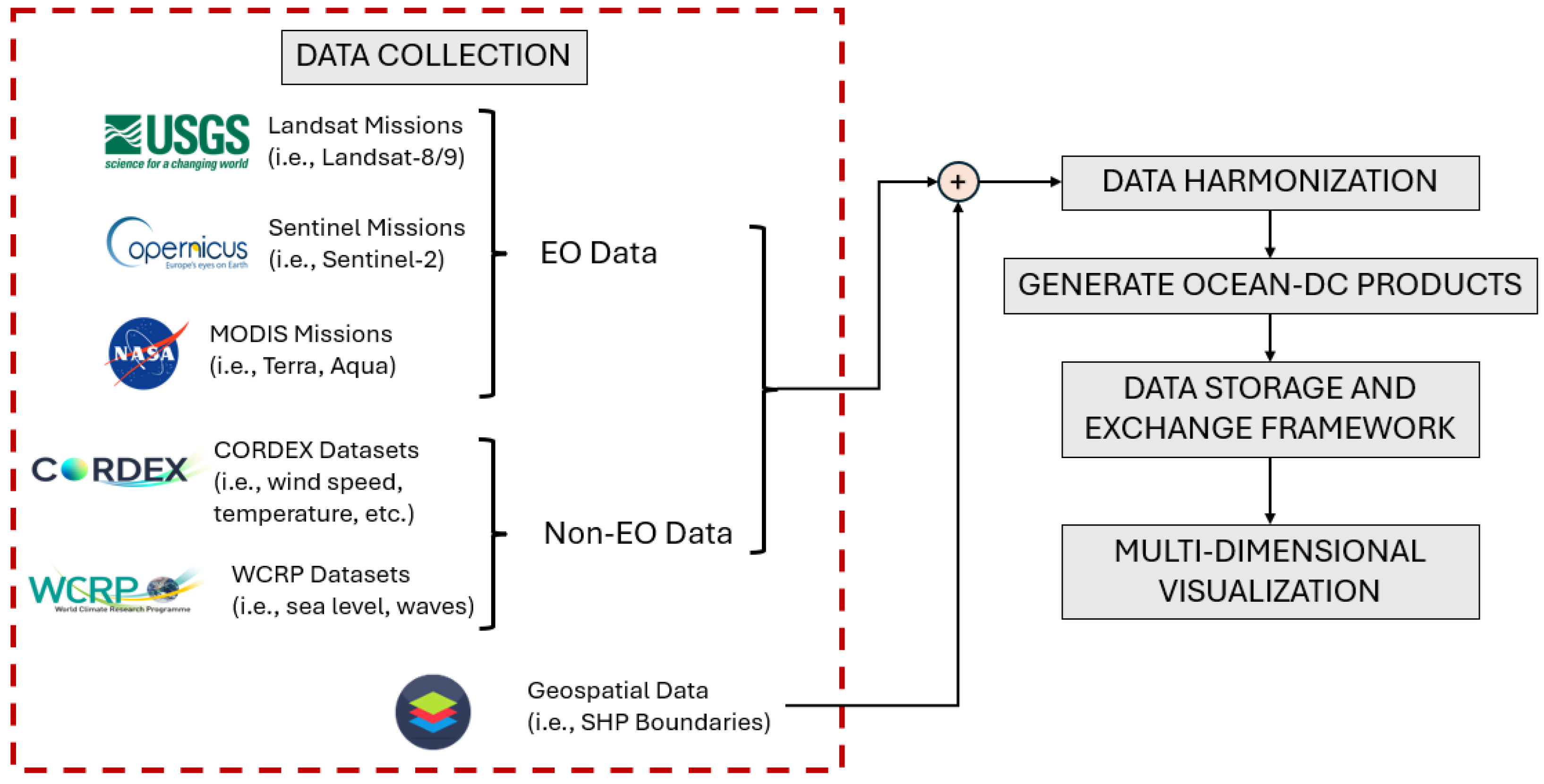
3.1. Data Collection

As previously mentioned, the Ocean-DC framework supports several kinds of data, both EO and non-EO data that can be used for coastal and maritime applications. First and foremost, the Ocean-DC framework is designed to process the EO raw data collected from different sources: (a) Landsat missions (i.e., 1–5 MSS, 4–5 TM, 7 ETM+, and 8–9 OLI-TIRS) from USGS [37]; (b) sentinel missions (i.e., Sentinel-1, Sentinel-2, Sentinel-3, Sentinel-5P) from Copernicus Data Space [38]; and (c) MODIS mission (i.e., TERRA, AQUA) from NASA [39].
In addition, the Ocean-DC framework processes non-EO data that includes seasonal/meteorological/data projections, waves and sea level parameters. These data are provided from CORDEX and WCRP data sources as time series. In addition, this category includes other types of data than can help in increasing the dimensionality of the final products to better enhance the results. Such data can be height maps (i.e., Digital Elevation Models (DEM) or Digital Terrain Models (DTM)) or bathymetry raster images. Moreover, shapefile polygons can be used as input to the harmonization stage for bounding the area of interest and clipping the original data (i.e., removing necessary information), leading to the storage of efficient products.
At this point, it is necessary to clarify that this study exclusively utilizes online data sources for collection. Table 1 presents compatible datasets with the Ocean-DC framework and their products. Although the Ocean-DC framework supports several datasets, the case study analysis of this manuscript uses Landsat and Sentinel products to demonstrate the frameworks’ utility, emphasizing Landsat-8/9 and Sentinel-2 products that contain similarities in radiometric information (i.e., spectral bands), and they are close in resolution. Moreover, it is necessary to mention that CORDEX projection data may be high resolution compared to other climate/meteorological data, but compared to remote sensing data, their resolution is low. For example, the selected area of interest for this case study (Port of Heraklion) expands to a 2 × 2 grid of CORDEX data. Thus, for being able to visualize them in a similar resolution as EO data, super-resolution processing is needed, which is out-of-scope for this research and is not supported in the current version of Ocean-DC. Similarly, the waves and sea level data are pointed, which follows a different post-processing from CORDEX and EO data.

3.2. Data Harmonization

The Ocean-DC framework deploys the open Python libraries Xarray [40], rioxarray [41], and rasterio [42] for data harmonization. The data harmonization phase integrates all essential processing steps for generating standardized Ocean-DC products. This comprehensive procedure involves (a) read data (applied to EO and non-EO data); (b) spatial clipping to the area of interest boundaries (applied to EO and non-EO data); (c) resampling all datasets to uniform spatial resolutions (applied to EO data); (d) reprojecting the products to a consistent Coordinate Reference System (CRS), where by default the WGS84 based on GRS80 ellipsoid with code EPSG:4326 (applied to EO and non-EO data) is used; (e) computing derived spectral indices and products commonly employed in remote sensing analysis (applied to EO and non-EO data); and (f) exporting the final data cubes in NetCDF format, which is a widely adopted standard for multidimensional scientific data storage and exchange (applied to EO and non-EO data). Figure 3 illustrates the harmonization phase steps for the EO data processing. This systematic approach ensures spatial and radiometric consistency across all processed datasets while maintaining compatibility with established geospatial analysis workflows.
As mentioned in the previous paragraphs, the Ocean-DC framework handles both EO and non-EO data under a similar architecture. However, the supported raw data are collected from different data sources, structured differently or distributed in totally different formats. Thus, the first step of the harmonization phase is to recognize the correct data type and execute the corresponding pipeline, which correctly reads the data and executes the necessary processes according to the data types. For example, while processing EO data, the first step is to identify the data origin from the missions identifier in the product’s name (i.e., S02 for Sentinel-2 products, L08 for Landsat-8 products, L09 for Landsat-9 products) as well as the product’s level processing that indicates the spectral information. For non-EO data, the Ocean-DC framework reads the data according to CORDEX [13] and WCRP [31] documentations.
During the clipping stage, the spatial extraction of the raw EO raster data is performed using the predefined shapefile boundary. This operation serves two critical purposes: (a) it significantly reduces data volume when processing small areas of interest for facilitating the efficient storage and distribution of final products; and (b) it establishes the spatial domain for subsequent processing steps. However, the output size exhibits non-linear growth relative to the dimensions of the area of interest, meaning that in some cases, the resulted Ocean-DC products can exceed the original file size when the clipping boundary represents large areas.
This size inflation occurs mainly in EO data because the harmonization process must resample all input radiometric bands, which are typically provided at varying spatial resolutions, to a common target resolution (generally the highest available resolution of the raw product, i.e., 10 m/px for Sentinel-2 products or 15 m/px for Landsat-8/9 products). Consequently, lower-resolution bands undergo substantial up-sampling during this standardization process, resulting in increased storage requirements for the final harmonized product. The clipping process is handled mainly from the Xarray library for the EO data. For non-EO data and especially CORDEX datasets, the clipping project is easier, as the resolution of the raw data expands to 156.25 km2, which is wide. In this case, the user specifies an output grid size (i.e., 2 × 2, 3 × 3, 4 × 4) and the algorithms find the coordinates of the central pixel (or bottom left closest in central pixel for 2 × 2, 4 × 4, etc., grid selections) and returns the corresponding values from the original datasets. Similarly, for WCRP data, the algorithm returns the information from the closest station point.
The resampling process (applied only to EO products) is applied to correct the different spatial resolutions between the spectral bands of raw EO products. This process is handled by rioxarray and rasterio libraries. The reshaping can be achieved in the lower, medium, or highest resolutions of the EO product if many spatial resolutions exist. For example, Landsat-8 products are distributed in 30 m/px spatial resolution for all spectral bands except panchromatic, which is in 15 m/px spatial resolution. In this case the higher resolution will up-sample all original bands from 30 m/px to 15 m/px by splitting the original 1-pixel to 4 pixels (twice the size). Similarly, for Sentinel-2 products, whose products are distributed in 10 m/px, 30 m/px, and 60 m/px spatial resolutions, some bands will be tripled or sextupled in size, and thus for larger areas, the final products will be increased in size.
The reprojection step defines the correct reference system for projecting correctly the Ocean-DC products with each other or with existing maps or other georeference data. Reprojection is succeeded by georeferencing the data to a user-defined CRS. By default, the system employs EPSG:4326 (World Geodetic System 1984-WGS84), which represents the global standard CRS commonly utilized in GPS applications. At this point it is worth mentioning that a critical consideration in this workflow is that the clipping geometry (i.e., shapefile boundary) may require prior reprojection to match the CRS of the input EO raster data, which is a mandatory step for the clipping operation to be properly executed. Given the computationally intensive nature of reprojection operations, it is significantly more efficient to perform this transformation on the shapefile geometry rather than on the complete EO raster dataset. This approach not only optimizes processing efficiency but also mitigates potential memory overflow issues that frequently arise when reprojecting large raster files.
Following reprojection, the Ocean-DC framework calculates several spectral indices commonly used in remote sensing applications. The automation of this integration provides an important advantage by delivering analysis-ready data, which can be immediately employed for coastal monitoring or other applications, without requiring high-demanding post-processing. However, it should be noted that these computational operations proportionally increase the final product size relative to the spatial extent of the clipping boundary. In cases involving large study areas, this may result in substantial file sizes that warrant consideration during storage planning and data distribution.
The harmonization phase ends by combining all derived products upon the original data, generating the Ocean-DC product. At this moment, the final product of the harmonization phase can be exported as NetCDF, which is an established standard for multidimensional scientific data storage and exchange. According to the application, the structure of a NetCDF file can be implemented using different architectural approaches. Precisely, for applications involving data distributions through sFTP networks with subsequent processing or visualization in GIS software (i.e., QGIS, ArcGIS, etc.) (i.e., QGIS), the NetCDF structure needs to mimic a Virtual Raster (VRT) template architecture. However, when geoserver compatibility is required, an alternative layered structure must be employed, where each spectral image is stored as a separate dataset within the NetCDF file due to the geoserver’s lack of a VRT-based architecture. This architectural flexibility allows the Ocean-DC framework to adapt to various deployment scenarios while maintaining data integrity and accessibility.

3.3. Post Processing and Storage Management
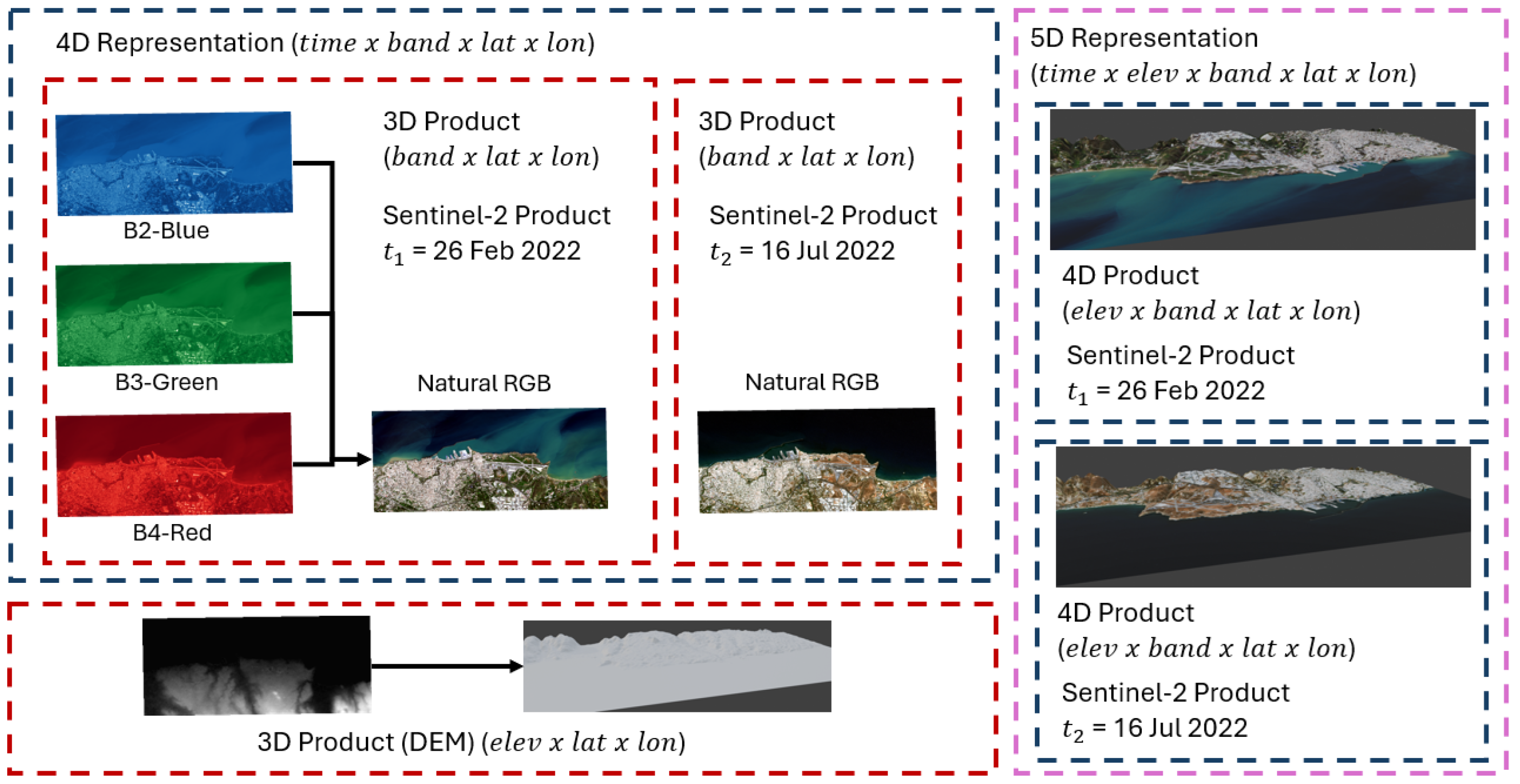
The Ocean-DC framework produces analysis-ready products through the aforementioned semi-automated processing steps, which are described in the previous paragraphs. This design allows users to focus exclusively on post-processing and data management tasks tailored to their exact application requirements. For example, in coastal monitoring application, post-processing primarily involves the generation of appropriate color palettes to provide effectiveness in the visualization of spectral indices or other EO products. In addition, the framework’s automated approach significantly reduces the preprocessing overhead while maintaining flexibility for parameter customization during the harmonization phase.
Another functionality of the Ocean-DC framework is the incorporation of the storage management within the harmonization phase, while maintaining user flexibility in data organization. The system automatically structures output products into directory hierarchies based on filename keywords, while the user retains full control over the physical storage location. Following product generation, distribution methods can be customized according to application needs, with options including sFTP transfer for complete dataset sharing or geoserver deployment for selective band distribution. While the framework facilitates these common distribution pathways, it remains compatible with external storage solutions such as cloud platforms or public servers, as these implementation-specific choices extend beyond the framework’s core functionality.

3.4. Visualization

The visualization of the Ocean-DC products is the final step of the proposed methodology. Today, there are several technologies that permit the visualization of high-dimensional data in various forms. To keep the analysis simple, this research compares traditional 3D ( b a n d × l a t i t u d e × l o n g i t u d e ) or 4D ( t i m e × b a n d × l a t i t u d e × l o n g i t u d e ) data structures with a 5D data structure, where as the 5th dimension, the elevation is considered. Thus, the final 5D data structure corresponds to the following dimensions ( t i m e × e l e v × b a n d × l a t i t u d e × l o n g i t u d e ) . Figure 2 illustrates a visual example of a dimension expanding for high-dimensional visualization.
Let use note that the generated Ocean-DC products are 3D ( b a n d × l a t i t u d e × l o n g i t u d e ) , similar to the original products. There are two ways to generate 4D data cubes (hyper cubes). The common and easiest approach is the comparison of two 3D data cubes, which is generated as a 4D ( t i m e × b a n d × l a t i t u d e × l o n g i t u d e ) representation. A different approach can be the generation of a 3D ( e l e v × l a t i t u d e × l o n g i t u d e ) Digital Elevation Model (DEM), which in this case, instead of radiometric information (i.e., spectral band), the 1st dimension corresponds to elevation. Thus, by applying the radiometric information upon the elevation model, a 4D ( e l e v × b a n d × l a t i t u d e × l o n g i t u d e ) product is generated. Please consider that this dimensional space can be equally expressed as ( b a n d × e l e v × l a t i t u d e × l o n g i t u d e ) , and the dimensional order affects only the architecture of the system. Finally, by combining two different temporal 4D products, a 5D ( t i m e × e l e v × b a n d × l a t i t u d e × l o n g i t u d e ) space is defined.
The visualization phase can be supported by a variety of software, such as GIS, 3D Editors or Game Engines. Each software provides a unique environment with the necessary tools for visualizing, editing, or navigating over the 3D spatial environment by either selecting different dates (4th dimension, i.e., time) or different spectral perspective (5th dimension, i.e., spectral band selection). For example, in QGIS software there are several plugins that can be used to transform a DEM into a 3D map, and the user can navigate to other dimensions by selecting different layers.
In a 3D Editor, such as Blender, the height-map can be used as a displacement map or modifier to transform a plane mesh to a realistic ground representation. In this case, the dimensions corresponding to the time and spectral bands are imported as mesh materials to the mesh geometry. Similarly, in a Game Engine, the 3D mesh geometry can be imported along with the images of spectral bands, which will be used as model materials. However, game engines support advanced graphic structures, lighting simulations, and a programming environment, which helps the user in developing realistic and interactive maps.
Further dimension expansion is also achievable by using climate, meteorological, or seasonal atmospheric data and advanced game engine graphics (i.e., fog) to project the information upon the current 4D ( e l e v × b a n d × l a t i t u d e × l o n g i t u d e ) model. Similarly, sea level rise or waves can be simulated inside a game engine, adding another dimensional parameter to the system. These applications can be built upon the Ocean-DC framework by post-processing the data cubes’ products. All these brainstorming ideas indicate the significance of the Ocean-DC framework as an emerging tool for addressing current Big Data challenges and bridging the gap between EO and non-EO analysis.

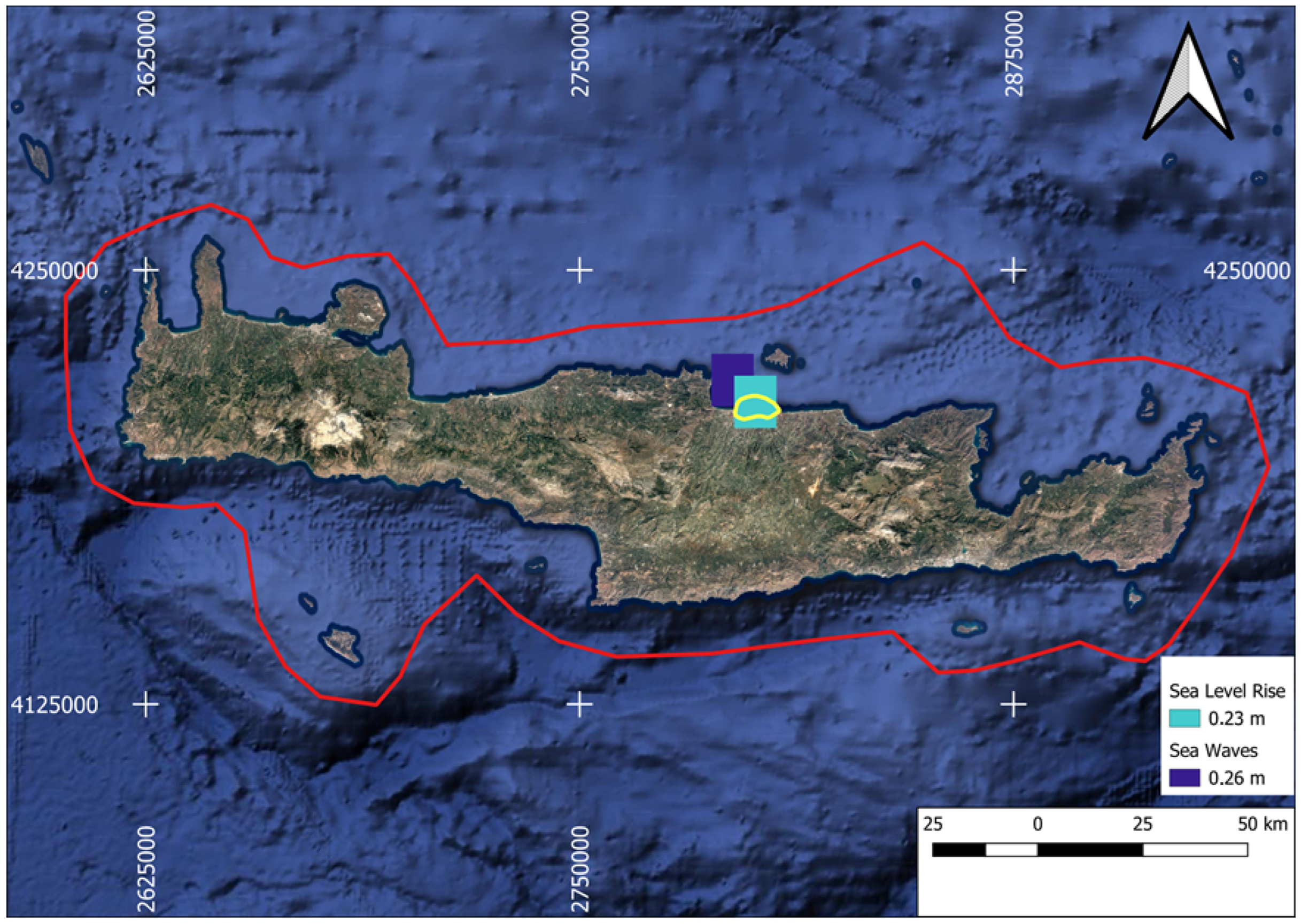
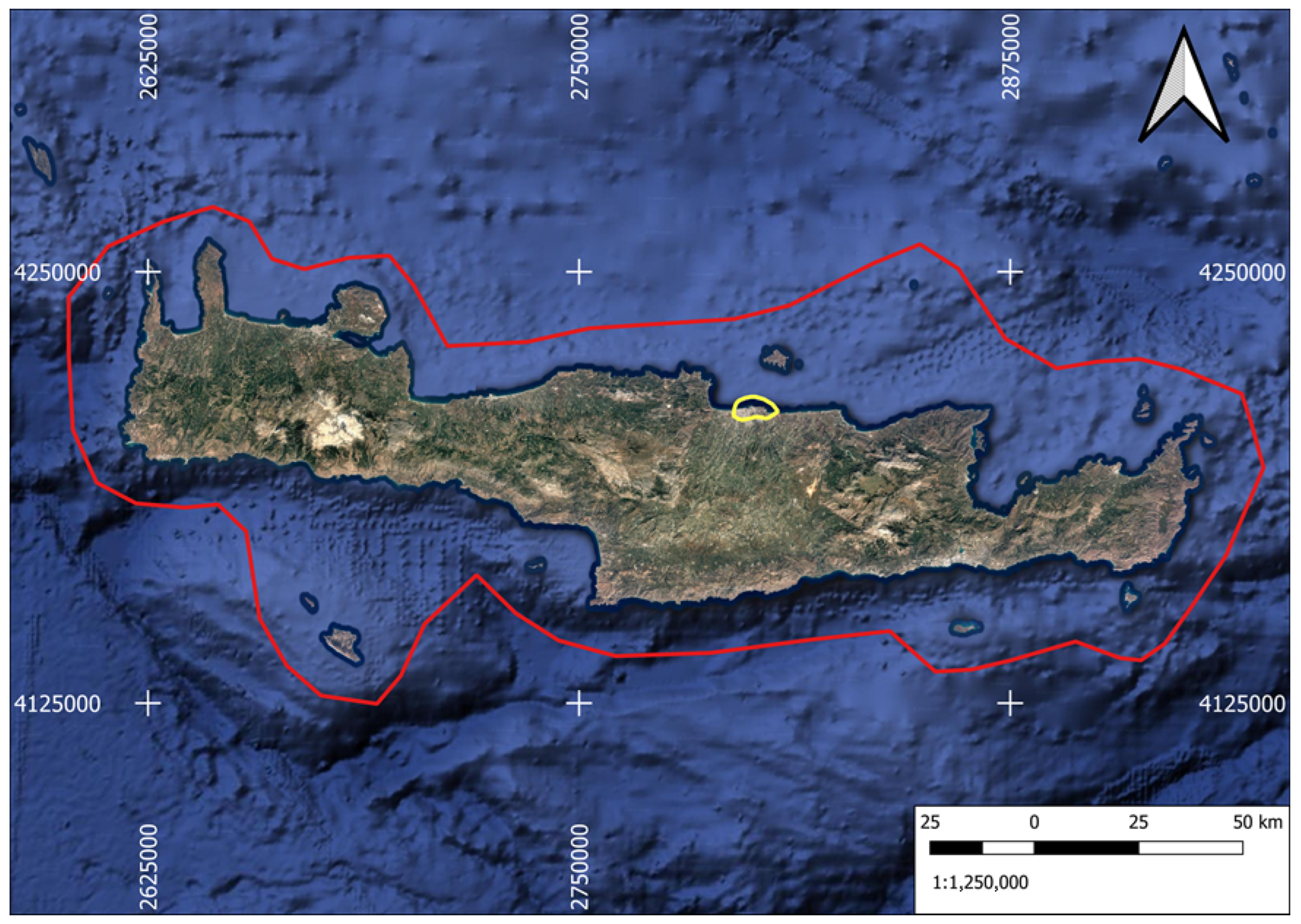
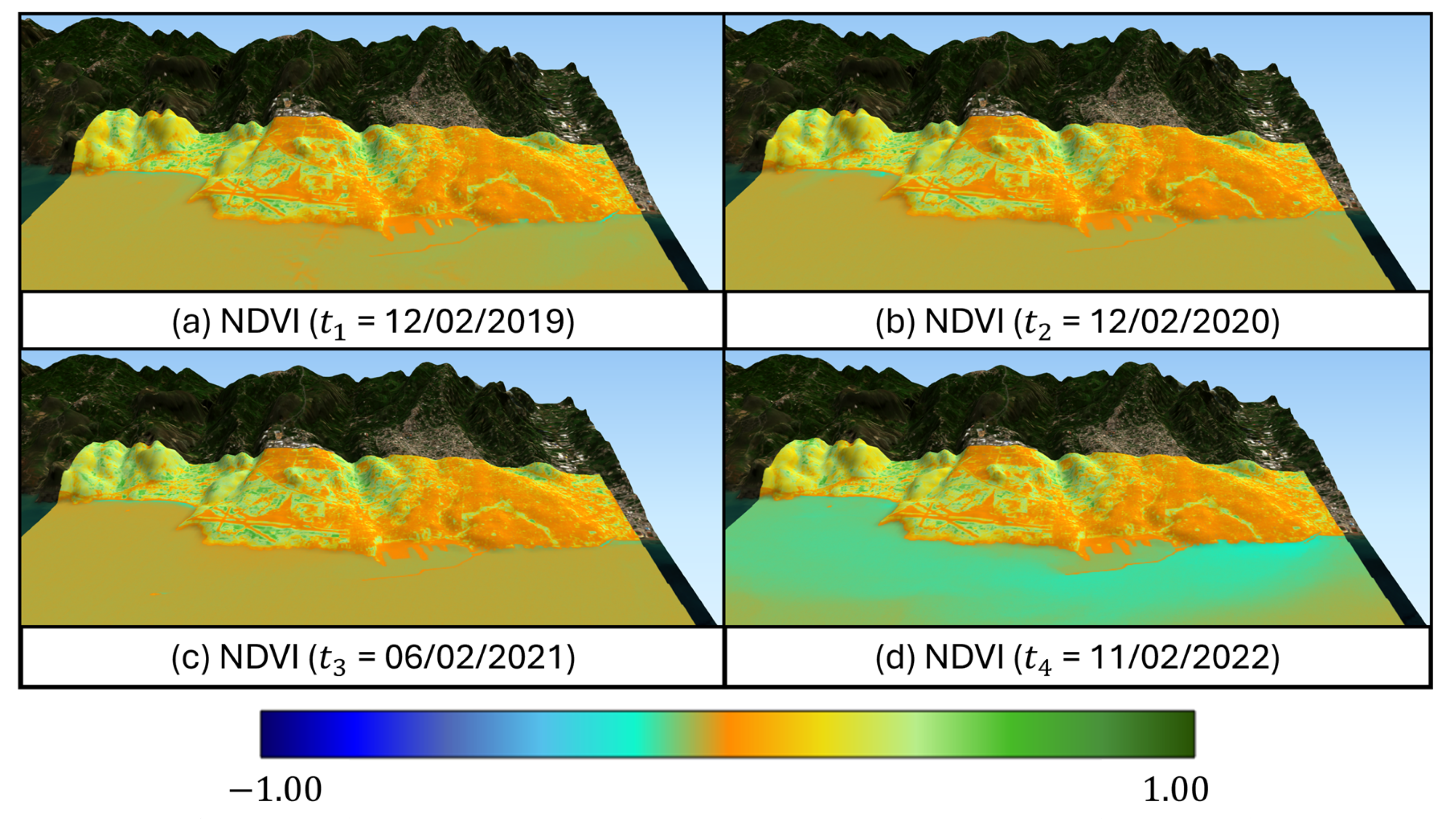
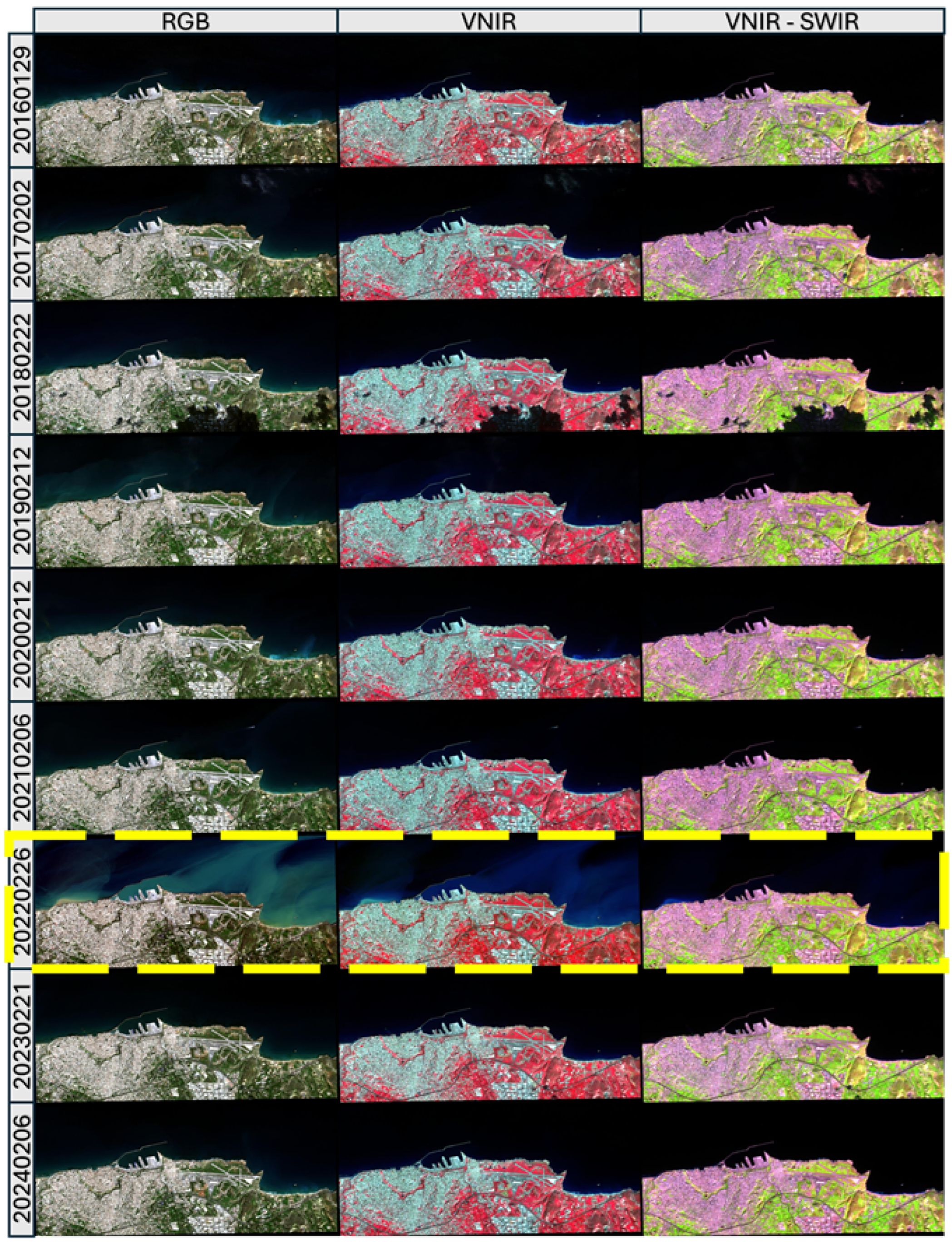
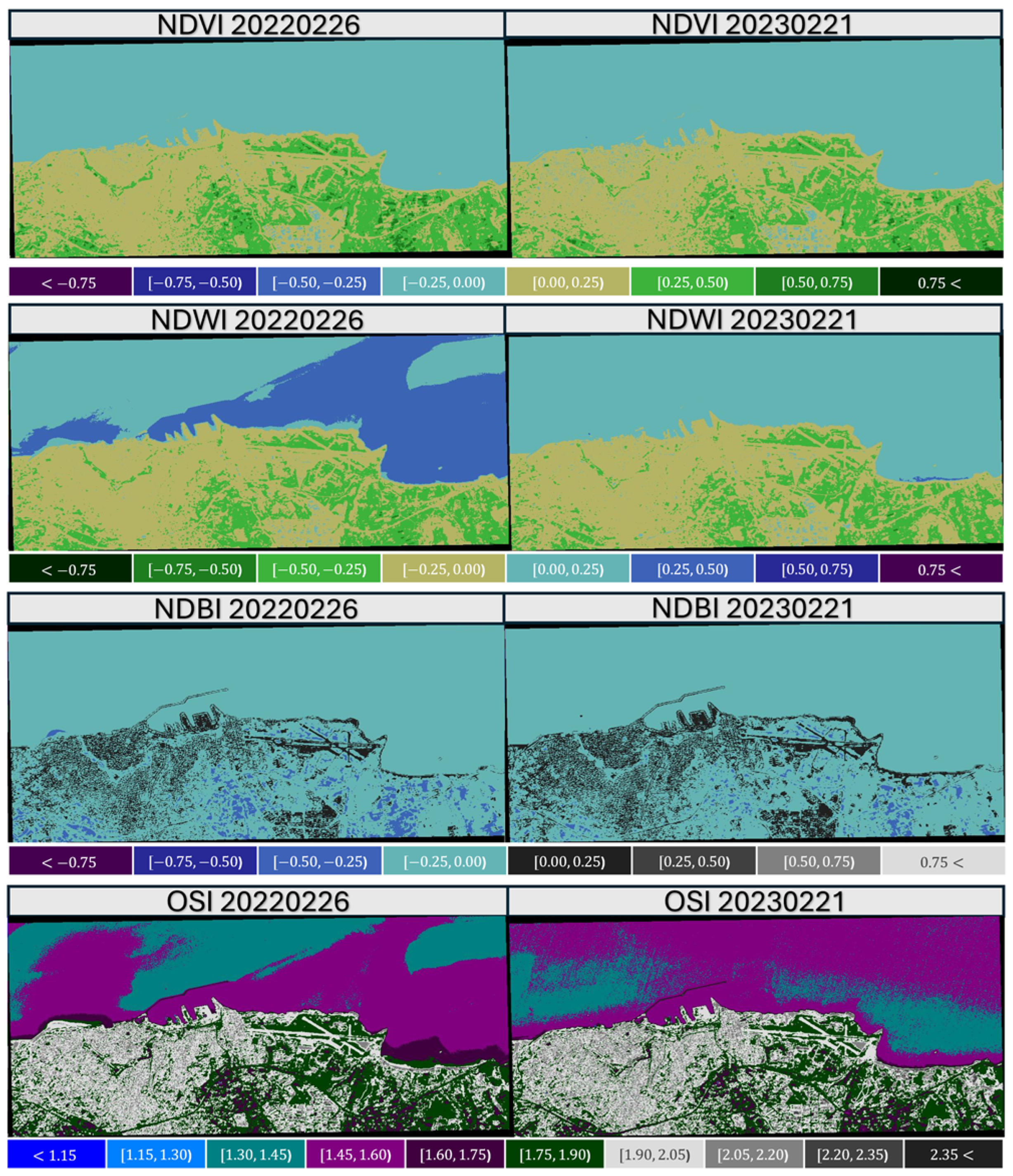
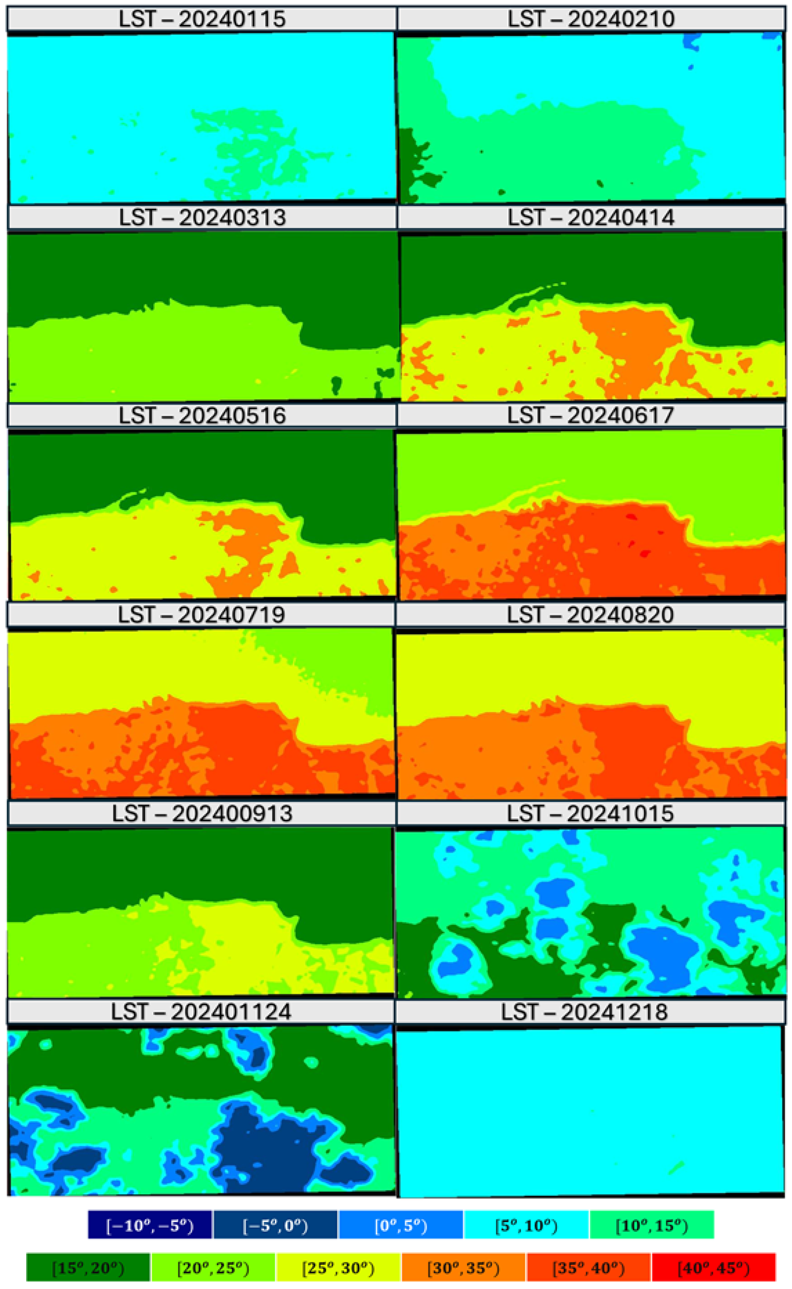
4. Case Study: Periodic Monitoring of the Port of Heraklion

The case study emphasizes the periodic monitoring of northern coastal regions of Crete Island, which are located in Greece, with particular emphasis on the Port of Heraklion and its surrounding areas. The Port of Heraklion is a critical hub for Crete’s blue economy, as the Heraklion Port Authority [43] manages the following principal maritime activities: (a) ferry operations; (b) cargo handling; (c) cruise tourism; (d) fishing harbor services; and (e) shipyard maintenance. These multifaceted operations underscore the port’s strategic economic importance while simultaneously increasing its vulnerability to coastal environmental changes that can impact maritime infrastructure and operations. The following sections describe in detail the experimental setup and results using the technologies described in the proposed methodology.

4.1. Experimental Setup

This work evaluates the efficacy of the Ocean-DC framework focusing on the tools and products for managing EO data and monitoring coastal regions through a systematic four-stage methodology. The proposed approach encompasses the following phases: (a) data collection; (b) data harmonization; (c) post-processing and storage management; and (d) visualization. Figure 3 presents the comprehensive workflow developed for EO product management and periodic coastal monitoring within this investigation. Please note that non-EO data like sea waves and sea level rise have lower resolution and need additional processing, which is out of scope for this research. Figure 4 provides a visual example of such data to clarify the reason why they are excluded from this case study example.
The Ocean-DC framework is publicly available on GitLab [44] as a cross-platform solution compatible with all major operating systems. Developed in Python, the framework can be readily deployed by installing the required dependencies within a Python virtual environment. This free and open-source implementation enables full reproducibility of the data harmonization pipeline, facilitating validation studies and collaborative development. The shared code-base allows researchers to replicate processing workflows, verify results, and adapt the framework for specific coastal monitoring applications.
In this experiment, we investigate the core environmental parameters that can be easily identified using remote sensing products and act as indicators for coastal degradation, especially in the Port of Heraklion. Considering the aforementioned variables, the data collection strategy is designed appropriately. Most of these variables can be visualized using EO data, such as Sentinel-2 and Landsat-8/9. Sentinel-2’s superior 10 m spatial resolution makes it ideal for coastal monitoring, though it lacks thermal bands for temperature analysis. For this reason, in this case study Sentinel-2 monthly data were downloaded from January 2016 to December 2024, and Landsat-8/9 monthly data were downloaded from January 2024 to December 2024 for thermal analysis and cross-sensor comparison. A significant challenge with both satellite systems is cloud interference, which can obscure critical ground data. For this reason, during the selection of the data, a filter is used with a cloud cover threshold of 60% to maximize the usable data while minimizing cloud obstruction.
Additional data includes the shapefile geometries that are used for clipping the EO data and representing the areas of interest. Figure 5 illustrates these boundaries: (a) The red boundary is used for clipping the images around Crete. (b) The yellow boundary is used for clipping the images around the Port of Heraklion. At this point, it is necessary to denote that if the boundary exceeds the EO images, then the clipping area will be decreased on that side to match the boundary of the image. In this case, the selected Sentinel-2 images have captured the northern coastal area of Crete island, and thus the analysis focuses on that area. Lastly, from the USGS Earth Explorer source, the SRTM 1 Arc-Second Global DEM of the Crete island was downloaded, which is used for generating the 3rd spatial dimension. Table 2 summarizes the datasets used in this case study.
The harmonization phase uses the tools of the Ocean-DC framework [45] for generating two types of data cubes: (a) layered data cubes compatible with Geoserver; and (b) VRT based data cubes for GIS software processing. Please note that these types of data cubes can be used in combination with each other for high-dimensional processing. For example, Figure 6 illustrates a 5D visualization of the NDVI time-series visualization in the Port of Heraklion from February 2019 to February 2022, indicating the potential of the proposed methodology. Please notice that the results are compared for the same season each year to exclude seasonal changes. In addition, in years 2019, 2020, and 2021, there is not a critical change, and thus it can be assumed a normal trend (pattern). However, in 2022 the water appears to be full of river debris, indicating critical conditions, which can cause coastal erosion and maritime degradation.
A different examination approach for providing similar results can be the generation of a mesh model inside a 3D editor and visualization of the Ocean-DC as a material texture. This alternative provides additional freedom, as 3D editors support tools and visualization features that GIS software does not include. An extension to the visualization inside a 3D editor, is the visualization and analysis inside a Game Engine environment, which supports programming, simulation and high-fidelity graphics (i.e., particle systems) which could be used to further expand the visualization dimensions. Though this extension could provide significant results, it is not investigated in this work but it is referred as an alternative option.

Evaluation Metrics

To evaluate the efficiency of the Ocean-DC framework for periodic coastal monitoring and compare it with the state-of-the-art approaches, we define five evaluation metrics:
  • Storage Ratio (SR): The SR is calculated by dividing the Ocean-DC product’s size with the raw product’s size, when both of these products contain the same spectral information (i.e., bands). This metric provides insights related to storage management.
  • Time Performance Ratio (TPR): This metric is calculated by comparing the time needed to calculate the products by standard methods (e.g., manual approach using GIS software or automation which exists in the GIS software).
  • Products Quality/Resolution (PQR = low, medium, high): This metric compares the products created from the Ocean-DC framework with those created products by standard methods. The quality estimated using photo interpretation techniques [46] (i.e., pattern recognition and color differences), which are commonly used in remote sensing.
  • Visualization Results (VisRes = low, medium, high): This metric evaluates the different dimensional products in terms of visualization. The evaluation criteria are the easiness of detection of the different entities (i.e., vegetation, urban, and coastal areas) in the images, without further processing. VisRes evaluated by using photo-interpretation techniques [46] similar to PQR.
  • Identifying Critical Conditions (ICC = easy, medium, hard): This metric is an extension of VisRes. In this case, different dates are visualized together for identifying trends related to seasonal or yearly changes and identifying the outliers or critical conditions of potential degradation based on photo-interpretation techniques [36,46].

4.2. Experimental Results

As described in the previous section, the main objective of this case study is to identify degradation in the northern coastal area of Crete island, emphasizing mostly in the surrounding area of the Port of Heraklion. By using the collected dataset, several EO products [28] were calculated using the Ocean-DC framework. However, according to the literature, the following products are the most suitable to monitor coastal degradation: (a) Visible Spectrum (RGB) [47]; (b) Visible Near Infrared (VNIR) [47]; (c) Visible Short-wave Infrared (VNIR-SWIR) [48]; (d) Thermal Infrared Products (i.e., Land Surface Temperature-LST) [48]; (e) Normalized Difference Vegetation Index (NDVI) [49,50]; (f) Normalized Difference Water Index (NDWI) [50,51]; (g) Normalized Difference Build-up Index (NDBI) [49,50] and Oil Spill Index (OSI) [52]; and (h) Normalized Difference Red Edge Index (NDRE) [50].
For the full dataset and each individual product (i.e., RGB, VNIR, NDVI, and NDWI), a total of 120 outputs were computed and visualized (12 for Landsat-8/9 and 108 for Sentinel-2) per clipping boundary. Using conventional remote sensing techniques and software, such as manual VRT generation and product calculation, the same processing for both clipping boundaries required an average of 90 min per dataset (i.e., a single Sentinel-2 or Landsat-8/9 raw product). In contrast, the Ocean-DC framework completed the same task in under 10 min. Consequently, the TPR metric is calculated as follows: T P R = 10 90 = 0.11 , which is 11% of the average time needed using traditional approaches (i.e., 89% less time).
Similarly, the following tables (Table 3 and Table 4) present the results of the SR metric for the clipping with the Port of Heraklion and Crete geometries, respectively. It is worth noting that small geometries (i.e., coastal monitoring in a small radius around the port) significantly reduce the storage size of the final products. However, in the opposite scenario, where it is needed to use big geometries (i.e., monitoring the whole northern coastal region of Crete), the storage size of the final products is increased by a lot. Thus, a recommended solution is to formulate the data and organize the storage in a suitable way to prevent storage memory overflowing.
Continuing the analysis, Figure 7 illustrates an example of periodic monitoring in the coastal area of Port of Heraklion. In this example, it is used in a yearly temporal window near February each year. By comparing the images together, it is easily identified that on 26 February 2022, there are a lot of river debris in the coastal area, which can cause possible degradation. Evaluating this 4D analysis (time × bands × lat × lon) based on VisRes criteria, the results provide high-quality material that make it easy to identify the critical conditions (i.e., the ICC metric is evaluated as easy).
Further analysis for estimating the magnitude of an extreme event uses EO indice products that are also provided in the Ocean-DC framework. Figure 8 compares the NDVI, NDWI, NDBI and OSI of 26 February 2022 (critical conditions with a lot of river debris in the coastal area) with 21 February 2023 (normal conditions, suitable for control image). The NDVI in both images is similar, with little differences in the agricultural area. In the NDWI products, the image of 26 February 2022, indicates the critical areas with higher values (dark blue). Similarly, on 21 February 2023, it appears that there is a small critical situation near the bay next to the airport. NDBI indicates some debris in the image of 26 February 2022. This index is used for highlighting the manufactured built-up areas (higher values) and mitigating the effects of terrain illumination (lower values). The debris is visualized with a blueish color, indicating ground material (probably dirt, gravel, and rocks) in the coastal area. Finally, the OSI index provides additional information about the water condition. In this index, the critical situation appears in the range of 1.60–1.75 (dark purple) values, which appear in the image of 26 February 2022, near the coastline. Clear or slightly dirty water appears between the range of 1.30 and 1.60 (1.30–1.45 clear, 1.45–1.60 slightly dirty).
The analysis so far expands the 3D Ocean-DC products to the 4th dimension, which is the temporal (time) dimension. However, 5D mapping (i.e., Time × DEM × Band × Lat × Lon), simulations of phenomena and serious games [53] for policy making and decision support systems [54] is an emerging trend. For this reason, it is necessary to investigate the feasibility of using Ocean-DC in combination with 3D models, the easiness of generating these models, and their final quality and resolution, which in this research is evaluated using the defined PQR metric.
Figure 9 provides an example of 5D visualization using QGIS. In this viewport, it is possible to select any point in 3D space and obtain its coordinates, while the value is estimated by its color. In the case study, for the background layer for the Crete region, the corresponding product of 26 February 2022 (critical conditions) is used, while the Port of Heraklion overlay is changed between 26 February 2022 and 21 February 2023. Of course, the variations are infinite, and the user has the freedom to select the combinations that satisfy the application.
Following the analysis and using photo-interpretation techniques to compare the images and considering as the control (normal) situation the date of 21 February 2023, the water regions with debris are clear enough only by the RGB composition. The other compositions visualize in high fidelity the debris around the river’s delta, pinpointing a critical region for possible erosion. In particular, the VNIR composition and the products NDWI and OSI indicate not only the debris close to the river’s delta but also the debris that has been spread in the maritime environment, which is identified using pattern recognition. Thus, in terms of the VizRes metric, the quality is high enough to indicate without using any specific technology the critical areas. Similarly, the ICC metric is high because the critical conditions are easily identified using simple pattern recognition and differences in color by applying the same color map to similar products.
Finally, using Landsat-8/9 products, it is possible to calculate the LST for identifying extreme temperatures that can affect the port infrastructure and cause material degradation. Figure 10 illustrates the monthly LST of 2024 calculated by the Ocean-DC framework. Please note that in the Port of Heraklio, during the summer months, the temperature is between 30 and 35 Celsius degrees, which is high. In addition, during October and November, lower temperatures are observed, with some areas indicating extremely low temperatures. Thus, the combination between LST products with others can provide a complete analysis for ocean degradation monitoring.
In terms of the PQR index, the quality of the products is high. In this case study, we restricted only in QGIS for visualizing the 5D DCs; however, as mentioned, other software can be used as well. Thus, summarizing the section, the proposed methodology is working, and the Ocean-DC framework can provide several data in a short time. This data can be post-processed or used as it is for creating multidimensional visualizations capable of indicating critical conditions that can cause coastal degradation.

5. Discussion

This work demonstrates the significant potential of the Ocean-DC framework for monitoring coastal surface degradation. In particular, the study emphasizes port environments, where infrastructures are highly exposed to environmental (i.e., temperature, humidity, and salinity) and anthropogenic (i.e., cargo management and cruiser/tourism/traveling activities) stressors. Through the integration of the Ocean-DC framework, the importance of data harmonization and the multidimensional structuring and visualization of EO products can facilitate scalable and time-efficient analysis of long-term trends related to coastal resilience.
The experimental results of the case study in Crete and Port of Heraklion underscore the added value of spatiotemporal analytics for the early detection of coastal degradation indicators. Both band combinations like Visible RGB, VNIR and VNIR-SWIR along with indices calculations like NDVI, NDWI, NDBI, and OSI provide reliable proxies in identification of seasonal changes, erosion patterns, vegetation changes and sedimentation anomalies, highlighting critical conditions. Notably, the 4D and 5D visualization capabilities of Ocean-DC allow for the intuitive interpretation of complex patterns across spatiotemporal and spectral dimensions that are critical for EWS and DSS in coastal management.
In addition, the evaluation metrics, and specifically the PQR, VisRes and ICC criteria, demonstrate that Ocean-DC products not only meet the standards required for operational use but in many cases exceed them. The detection of extreme coastal events (e.g., river debris accumulation in February 2022) is immediate and visually discernible without additional processing, validating the effectiveness of the framework’s automated processing and visualization pipeline. Furthermore, in terms of time (TPR) the Ocean-DC framework can accelerate processing analysis up to 89% by semi-automating the whole calculation/visualization processes (the user only needs to create the color maps and select which parameters they want to visualize). In terms of storage management, the Ocean-DC framework can efficiently handle the creation of data for small regions; however, for larger areas (i.e., the northern region of Crete), the product size is hugely expanded. This limitation can cause serious storage issues (i.e., memory overflow), and thus it is not recommended to use this process analysis for large areas.
Finally, this work aligns with the broader literature in remote sensing and environmental analytics, emphasizing the transition from static observation to dynamic and predictive monitoring. The Ocean-DC framework contributes to this transition by offering a generalized, adaptable and on-the-fly system, which can be integrated with several kinds of data. The Ocean-DC framework was developed mainly for ocean and coastal applications, especially near port areas, but in reality, it can be used for other applications as well (i.e., vegetation monitoring, deforestation monitoring, and urbanism monitoring). In addition, it can work well with artificial learning and machine learning applications, as the Ocean-DC products can be used for input/output with little to zero post-processing.
Thus, future work will focus on enhancing the Ocean-DC framework through integration with predictive models and real-time data streams, while expanding its application to other sensitive coastal zones. Higher visualization dimensionality will also be investigated, possibly through simulations.

6. Conclusions

In this work, we investigated and validated the potential of Ocean-DC framework as a robust, modular and scalable approach for big data harmonization, processing and visualization of coastal degradation. By integrating Sentinel-2 and Landsat-8/9 imagery with temporal, spectral, and elevation dimensions, Ocean-DC enables advanced monitoring capabilities, which extend beyond conventional remote sensing workflows. In addition, Ocean-DC products comply with general industry standards and are interoperable with mainstream GIS software (e.g., QGIS, ArcGIS) or shareable via open-source platforms such as GeoServer.
The case study in the Port of Heraklion demonstrated the system’s operational readiness, while revealing significant environmental patterns through the automation of remote sensing indices calculation and multidimensional visualization. Ocean-DC products successfully identified key indicators of degradation, such as seasonal wetland variations, shoreline vegetation loss, sediment transport, river debris, and heat anomalies. In addition, the integration of DEM layers further enhanced the spatial fidelity of the monitoring outputs, allowing for advanced 5D representations.
In terms of performance, the framework achieved a substantial reduction in processing time and provided structured data products suitable for downstream analysis and dissemination. These findings support the framework’s application in broader geospatial contexts, including environmental resilience, climate impact assessment, and maritime spatial planning. Overall, this work provides a replicable, open-source foundation for EO-based environmental intelligence, contributing to informed decision-making in coastal management and infrastructure sustainability.
By concluding this work, the main insight and conclusions are summarized as follows:
  • This work presents the Ocean-DC framework as an emerging technology comparable to current state-of-the-art data cubes’ generators like Google Earth Engine and Open Data Cubes.
  • In comparison with the state-of-the-art data cubes’ generators, the Ocean-DC framework is supported by all major OS and can be installed easily in any system, even in virtual machines. In addition, it supports the processing of CORDEX and WCRP datasets without preprocessing.
  • In terms of the output products, the Ocean-DC generates ready-to-use data cubes in NetCDF format without necessarily needing post-processing. The generated EO products can be accesses, shared, and visualized easily in any GIS software as VRTs or a geoserver via standardized formats (i.e., WMS/WFS).
  • A limitation to the current Ocean-DC product can be the unavailability to upscale (i.e., super-resolution) the CORDEX and WCRP data, which need further processing outside the framework.
  • For both EO and non-EO data, the Ocean-DC framework uses boundary geometries to clip the original data over the area of interest (i.e., exclude unnecessary information). A natural limitation to this process can be the selection of huge areas of interest, which can increase the storage size of final products compared to the raw structure.
  • While processing EO data, the Ocean-DC framework calculates several remote sensing products automatically by recognizing the correct data type. This characteristic severely minimizes the needed post-processing time (or download time if using current existing alternatives to obtain similar ready-to-use data).
  • Considering the case study results, the Ocean-DC framework can be an intuitive solution for ocean and maritime periodic monitoring, as the generated products can be visualized using different multidimensional analysis approaches, such as photo-interpretation like pattern recognition, differences in colors, etc. In these approaches, the correct selection of a color map can indicate successfully critical areas and extreme situations that can cause coastal and maritime degradation.

Author Contributions

Conceptualization, I.K., I.R., N.B. and A.D.; Methodology, I.K. and N.B.; Software, I.K.; Validation, I.K.; Resources, A.D.; Writing, I.K.; Visualization, I.K.; Supervision, I.K.; Project administration, A.D.; Funding acquisition, A.D. All authors have read and agreed to the published version of the manuscript.

Funding

This work is supported by the European Union Funded project OCEANIDS “User-driven applications and tools for Climate-Informed Maritime Spatial Planning and integrated seascape management, towards a resilient & inclusive Blue Economy”, under the EU HE research and innovation program under GA No. 101112919.

Data Availability Statement

The data for this research were downloaded from USGS Earth Explorer and Copernicus Data Space. The code and visualization products can be found in https://gitlab.com/JohnCrabs/oceanids-data-cube-app (accessed on 23 June 2025). Ocean-DC product examples can be found on Zenodo (https://zenodo.org/records/15582751) (accessed on 23 June 2025).

Conflicts of Interest

The authors declare no conflicts of interest.

References

  1. Halder, B.; Ameen, A.M.S.; Bandyopadhyay, J.; Khedher, K.M.; Yaseen, Z.M. The impact of climate change on land degradation along with shoreline migration in Ghoramara Island, India. Phys. Chem. Earth Parts A/B/C 2022, 126, 103135. [Google Scholar] [CrossRef]
  2. Guerra-Mera, J.C.; Sabando García, Á.R.; Pin-Mera, M.G.; Rodríguez-Díaz, J.M.; Castañeda-Valdés, A. Assessment of atmospheric corrosivity in coastal zones: Case study in port Lopez, Manabí, Ecuador. Case Stud. Chem. Environ. Eng. 2024, 9, 100703. [Google Scholar] [CrossRef]
  3. Petrişor, A.I.; Hamma, W.; Nguyen, H.D.; Randazzo, G.; Muzirafuti, A.; Stan, M.I.; Tran, V.T.; Aştefănoaiei, R.; Bui, Q.T.; Vintilă, D.F.; et al. Degradation of Coastlines under the Pressure of Urbanization and Tourism: Evidence on the Change of Land Systems from Europe, Asia and Africa. Land 2020, 9, 275. [Google Scholar] [CrossRef]
  4. Andrews, N.; Bennett, N.J.; Le Billon, P.; Green, S.J.; Cisneros-Montemayor, A.M.; Amongin, S.; Gray, N.J.; Sumaila, U.R. Oil, fisheries and coastal communities: A review of impacts on the environment, livelihoods, space and governance. Energy Res. Soc. Sci. 2021, 75, 102009. [Google Scholar] [CrossRef]
  5. Mejjad, N.; Rossi, A.; Pavel, A.B. The coastal tourism industry in the Mediterranean: A critical review of the socio-economic and environmental pressures & impacts. Tour. Manag. Perspect. 2022, 44, 101007. [Google Scholar] [CrossRef]
  6. Bethel, B.J.; Buravleva, Y.; Tang, D. Blue Economy and Blue Activities: Opportunities, Challenges, and Recommendations for The Bahamas. Water 2021, 13, 1399. [Google Scholar] [CrossRef]
  7. Fudge, M.; Ogier, E.; Alexander, K.A. Marine and coastal places: Wellbeing in a blue economy. Environ. Sci. Policy 2023, 144, 64–73. [Google Scholar] [CrossRef]
  8. Apostolopoulos, D.; Nikolakopoulos, K. A review and meta-analysis of remote sensing data, GIS methods, materials and indices used for monitoring the coastline evolution over the last twenty years. Eur. J. Remote Sens. 2021, 54, 240–265. [Google Scholar] [CrossRef]
  9. Vitousek, S.; Buscombe, D.; Vos, K.; Barnard, P.L.; Ritchie, A.C.; Warrick, J.A. The future of coastal monitoring through satellite remote sensing. Camb. Prism. Coast. Futures 2023, 1, e10. [Google Scholar] [CrossRef]
  10. Chen, J.; Chen, S.; Fu, R.; Li, D.; Jiang, H.; Wang, C.; Peng, Y.; Jia, K.; Hicks, B.J. Remote Sensing Big Data for Water Environment Monitoring: Current Status, Challenges, and Future Prospects. Earth Future 2022, 10, e2021EF002289. [Google Scholar] [CrossRef]
  11. Google. Google Earth Engine. 2025. Available online: https://earthengine.google.com/ (accessed on 23 June 2025).
  12. Open Data Cubes Team. Open Data Cubes. 2025. Available online: https://www.opendatacube.org/ (accessed on 23 June 2025).
  13. CORDEX. Coordinate Regional Climate Downscaling Experiment. 2025. Available online: https://cordex.org/ (accessed on 23 June 2025).
  14. Sarawagi, S.; Agrawal, R.; Megiddo, N. Discovery-driven exploration of OLAP data cubes. In Proceedings of the Advances in Database Technology—EDBT’98: 6th International Conference on Extending Database Technology, Valencia, Spain, 23–27 March 1998; Proceedings 6. Springer: Berlin/Heidelberg, Germany, 1998; pp. 168–182. [Google Scholar]
  15. Gray, J.; Chaudhuri, S.; Bosworth, A.; Layman, A.; Reichart, D.; Venkatrao, M.; Pellow, F.; Pirahesh, H. Data cube: A relational aggregation operator generalizing group-by, cross-tab, and sub-totals. Data Min. Knowl. Discov. 1997, 1, 29–53. [Google Scholar] [CrossRef]
  16. Francia, M.; Marcel, P.; Peralta, V.; Rizzi, S. Enhancing cubes with models to describe multidimensional data. Inf. Syst. Front. 2022, 24, 31–48. [Google Scholar] [CrossRef]
  17. Leprince, J.; Miller, C.; Zeiler, W. Data mining cubes for buildings, a generic framework for multidimensional analytics of building performance data. Energy Build. 2021, 248, 111195. [Google Scholar] [CrossRef]
  18. Song, Y.; Fan, Y.; Li, X.; Ji, Y. Multidimensional visualization of transit smartcard data using space–time plots and data cubes. Transportation 2018, 45, 311–333. [Google Scholar] [CrossRef]
  19. Giuliani, G.; Chatenoux, B.; Benvenuti, A.; Lacroix, P.; Santoro, M.; Mazzetti, P. Monitoring land degradation at national level using satellite Earth Observation time-series data to support SDG15–exploring the potential of data cube. Big Earth Data 2020, 4, 3–22. [Google Scholar] [CrossRef]
  20. Miranda, F.; Lins, L.; Klosowski, J.T.; Silva, C.T. Topkube: A rank-aware data cube for real-time exploration of spatiotemporal data. IEEE Trans. Vis. Comput. Graph. 2017, 24, 1394–1407. [Google Scholar] [CrossRef]
  21. Tardío, R.; Maté, A.; Trujillo, J. A new big data benchmark for OLAP cube design using data pre-aggregation techniques. Appl. Sci. 2020, 10, 8674. [Google Scholar] [CrossRef]
  22. Majeed, A.; Zhang, Y.; Ren, S.; Lv, J.; Peng, T.; Waqar, S.; Yin, E. A big data-driven framework for sustainable and smart additive manufacturing. Robot.-Comput.-Integr. Manuf. 2021, 67, 102026. [Google Scholar] [CrossRef]
  23. Ferreira, K.R.; Queiroz, G.R.; Vinhas, L.; Marujo, R.F.B.; Simoes, R.E.O.; Picoli, M.C.A.; Camara, G.; Cartaxo, R.; Gomes, V.C.F.; Santos, L.A.; et al. Earth Observation Data Cubes for Brazil: Requirements, Methodology and Products. Remote Sens. 2020, 12, 4033. [Google Scholar] [CrossRef]
  24. Poussin, C.; Guigoz, Y.; Palazzi, E.; Terzago, S.; Chatenoux, B.; Giuliani, G. Snow Cover Evolution in the Gran Paradiso National Park, Italian Alps, Using the Earth Observation Data Cube. Data 2019, 4, 138. [Google Scholar] [CrossRef]
  25. Chatenoux, B.; Richard, J.P.; Small, D.; Roeoesli, C.; Wingate, V.; Poussin, C.; Rodila, D.; Peduzzi, P.; Steinmeier, C.; Ginzler, C.; et al. The Swiss data cube, analysis ready data archive using earth observations of Switzerland. Sci. Data 2021, 8, 295. [Google Scholar] [CrossRef]
  26. Giuliani, G.; Chatenoux, B.; Piller, T.; Moser, F.; Lacroix, P. Data Cube on Demand (DCoD): Generating an earth observation Data Cube anywhere in the world. Int. J. Appl. Earth Obs. Geoinf. 2020, 87, 102035. [Google Scholar] [CrossRef]
  27. Lewis, A.; Oliver, S.; Lymburner, L.; Evans, B.; Wyborn, L.; Mueller, N.; Raevksi, G.; Hooke, J.; Woodcock, R.; Sixsmith, J.; et al. The Australian Geoscience Data Cube—Foundations and lessons learned. Remote Sens. Environ. 2017, 202, 276–292. [Google Scholar] [CrossRef]
  28. Kavouras, I.; Rallis, I.; Doulamis, N.; Doulamis, A. Ocean-DC: An analysis ready data cube framework for environmental and climate change monitoring over the port areas. In Proceedings of the 17th International Conference on PErvasive Technologies Related to Assistive Environments, Crete, Greece, 26–28 June 2024; pp. 412–419. [Google Scholar]
  29. EU Commission. HORIZON EUROPE, OCEANIDS Project: User-Driven Applications and Tools for Climate-Informed Maritime Spatial Planning and Integrated Seascape Management, Towards a Resilient & Inclusive Blue Economy. 2025. Available online: https://cordis.europa.eu/project/id/101112919 (accessed on 23 June 2025).
  30. European Commission. Variables that Could Be Useful for Managing Coastal Erosion-Suggestions from Nic Flemming. 2025. Available online: https://maritime-forum.ec.europa.eu/contents/variables-could-be-useful-managing-coastal-erosion-suggestions-nic-flemming_en?prefLang=sv (accessed on 23 June 2025).
  31. WCRP. World Climate Research Program. 2025. Available online: https://www.wcrp-climate.org/ (accessed on 23 June 2025).
  32. Carvalho, M.; Cardoso-Fernandes, J.; González, F.J.; Teodoro, A.C. Comparative Performance of Sentinel-2 and Landsat-9 Data for Raw Materials’ Exploration Onshore and in Coastal Areas. Remote Sens. 2025, 17, 305. [Google Scholar] [CrossRef]
  33. GEBCO-British Oceanographic Data Centre. Gridded Bathymetry Data. 2025. Available online: https://www.gebco.net/data-products/gridded-bathymetry-data (accessed on 23 June 2025).
  34. Marzialetti, F.; Giulio, S.; Malavasi, M.; Sperandii, M.G.; Acosta, A.T.R.; Carranza, M.L. Capturing Coastal Dune Natural Vegetation Types Using a Phenology-Based Mapping Approach: The Potential of Sentinel-2. Remote Sens. 2019, 11, 1506. [Google Scholar] [CrossRef]
  35. Sebastiá-Frasquet, M.T.; Aguilar-Maldonado, J.A.; Santamaría-Del-Ángel, E.; Estornell, J. Sentinel 2 Analysis of Turbidity Patterns in a Coastal Lagoon. Remote Sens. 2019, 11, 2926. [Google Scholar] [CrossRef]
  36. Filippucci, P.; Brocca, L.; Bonafoni, S.; Saltalippi, C.; Wagner, W.; Tarpanelli, A. Sentinel-2 high-resolution data for river discharge monitoring. Remote Sens. Environ. 2022, 281, 113255. [Google Scholar] [CrossRef]
  37. USGS. EarthExplorer. 2025. Available online: https://earthexplorer.usgs.gov/ (accessed on 23 June 2025).
  38. EU, Copernicus, ESA. Copernicus Data Space. 2025. Available online: https://dataspace.copernicus.eu/ (accessed on 23 June 2025).
  39. NASA. MODIS Data. 2025. Available online: https://modis.gsfc.nasa.gov/data/ (accessed on 23 June 2025).
  40. Xarray. Xarray Documentation. 2024. Available online: https://docs.xarray.dev/en/stable/ (accessed on 23 June 2025).
  41. Corteva Agriscience. Rioxarray Documentation. 2025. Available online: https://corteva.github.io/rioxarray/stable/ (accessed on 23 June 2025).
  42. Rasterio Team. Rasterio Documentation. 2025. Available online: https://rasterio.readthedocs.io/en/stable/ (accessed on 23 June 2025).
  43. Heraklion Port Authority, S.A. Heraklion Port Authority. 2025. Available online: https://portheraklion.gr/index.php/en/ (accessed on 23 June 2025).
  44. Kavouras, I. Oceanids Data Cubes Code. 2025. Available online: https://gitlab.com/JohnCrabs/oceanids-data-cube-app (accessed on 23 June 2025).
  45. JohnCrabs. Ocean-DC Framework. 2024. Available online: https://gitlab.com/JohnCrabs/oceanides_data_cubes/-/tree/main/src?ref_type=heads (accessed on 23 June 2025).
  46. Bianchetti, R.A.; MacEachren, A.M. Cognitive Themes Emerging from Air Photo Interpretation Texts Published to 1960. Isprs Int. J.-Geo-Inf. 2015, 4, 551–571. [Google Scholar] [CrossRef]
  47. Acuña-Ruz, T.; Uribe, D.; Taylor, R.; Amézquita, L.; Guzmán, M.C.; Merrill, J.; Martínez, P.; Voisin, L.; Mattar B., C. Anthropogenic marine debris over beaches: Spectral characterization for remote sensing applications. Remote Sens. Environ. 2018, 217, 309–322. [Google Scholar] [CrossRef]
  48. Milewski, R.; Schmid, T.; Chabrillat, S.; Jiménez, M.; Escribano, P.; Pelayo, M.; Ben-Dor, E. Analyses of the Impact of Soil Conditions and Soil Degradation on Vegetation Vitality and Crop Productivity Based on Airborne Hyperspectral VNIR–SWIR–TIR Data in a Semi-Arid Rainfed Agricultural Area (Camarena, Central Spain). Remote Sens. 2022, 14, 5131. [Google Scholar] [CrossRef]
  49. de Araújo Queiroz, H.A.; Gonçalves, R.M.; Mishra, M. Characterizing global satellite-based indicators for coastal vulnerability to erosion management as exemplified by a regional level analysis from Northeast Brazil. Sci. Total Environ. 2022, 817, 152849. [Google Scholar] [CrossRef] [PubMed]
  50. C, S.; Alsolai, H.; Allafi, R.; Arasi, M.A. Integrated image segmentation techniques for high-resolution coastal habitat mapping: Advancing remote sensing for coastal ecosystem assessment. J. South Am. Earth Sci. 2025, 159, 105526. [Google Scholar] [CrossRef]
  51. Wicaksono, A.; Wicaksono, P. Geometric accuracy assessment for shoreline derived from NDWI, MNDWI, and AWEI transformation on various coastal physical typology in Jepara Regency using Landsat 8 OLI imagery in 2018. Geoplanning J. Geomat. Plan 2019, 6, 55–72. [Google Scholar] [CrossRef]
  52. Balogun, A.L.; Yekeen, S.T.; Pradhan, B.; Althuwaynee, O.F. Spatio-Temporal Analysis of Oil Spill Impact and Recovery Pattern of Coastal Vegetation and Wetland Using Multispectral Satellite Landsat 8-OLI Imagery and Machine Learning Models. Remote Sens. 2020, 12, 1225. [Google Scholar] [CrossRef]
  53. Kavouras, I.; Sardis, E.; Protopapadakis, E.; Rallis, I.; Doulamis, A.; Doulamis, N. A Low-Cost Gamified Urban Planning Methodology Enhanced with Co-Creation and Participatory Approaches. Sustainability 2023, 15, 2297. [Google Scholar] [CrossRef]
  54. Kavouras, I.; Rallis, I.; Sardis, E.; Protopapadakis, E.; Doulamis, A.; Doulamis, N. Empowering Communities Through Gamified Urban Design Solutions. Smart Cities 2025, 8, 44. [Google Scholar] [CrossRef]
Figure 1. The Ocean-DC framework architecture.
Jmse 13 01239 g001
Figure 2. Example of a dimension expanding for high-dimensional visualization.
Jmse 13 01239 g002
Figure 3. The suggested workflow for EO products’ management and periodic coastal region monitoring based on high-dimensional Ocean-DC products.
Jmse 13 01239 g003
Figure 4. Mapping example of sea level rising and sea waves. The Ocean-DC products contain time-series geolocated information, which cannot be efficiently visualized in a 2D map, without further processing. The center point of each square corresponds to the location of the measured station, while the size of the square has no physical meaning and is used only for visualization purposes. Red boundary is used for clipping the whole Crete island. Yellow boundary is used for clipping the coastal area around the Port of Heraklion. (source of map background: Google Satellite, projection: EPSG3857/WGS84-Pseudo Mercator).
Jmse 13 01239 g004
Figure 5. Polygon geometries of selected areas of interest. Red boundary is used for clipping the whole Crete island. Yellow boundary is used for clipping the coastal area around the Port of Heraklion. (source of map background: Google Satellite, projection: EPSG3857/WGS84-Pseudo Mercator).
Jmse 13 01239 g005
Figure 6. A 5D ( t i m e × e l e v × b a n d × l a t i t u d e × l o n g i t u d e ) visualization of the NDVI time-series visualization in the Port of Heraklion from February 2019 to February 2022.
Jmse 13 01239 g006
Figure 7. Example of periodic monitoring in the coastal area of the Port of Heraklion, using a yearly temporal window near February each year. The yellow boundary indicates critical condition and possible degradation in the coastal area.
Jmse 13 01239 g007
Figure 8. Comparison between the products of 26 February 2022 (critical conditions) and 21 February 2023 (normal conditions).
Jmse 13 01239 g008
Figure 9. A 5D ( t i m e × e l e v × b a n d × l a t i t u d e × l o n g i t u d e ) visualization of Ocean-DC products inside QGIS.
Jmse 13 01239 g009
Figure 10. Land Surface Temperature 4D ( t i m e × b a n d × l a t i t u d e × l o n g i t u d e ) monitoring using Landsat-8/9 products.
Jmse 13 01239 g010
Table 1. Datasets that can be used with the current version of the Ocean-DC framework.
Data TypeProduct NameDescriptionResolutionData Source
EOLandsat MissionLandsat missions, operating since 1972, provide continuous Earth observation data, capturing multispectral and thermal imagery. They can be used to monitor coastlines, map habitats like mangroves, assess water quality (e.g., turbidity, chlorophyll), and track temperature anomalies. With free, long-term data, Landsat supports sustainable marine management.Moderate resolution (15 m/px, 30 m/px, 100 m/px)USGS [37]
EOSentinel MissionThe Sentinel missions, part of ESA’s Copernicus program, deliver high-resolution Earth observation data. Sentinel-2 maps coastal land cover and water quality, while Sentinel-3 monitors sea surface temperature and ocean color. Their frequent revisits and open data support shoreline tracking, sediment plume detection, and algal bloom monitoring.Moderate to High resolutions (5 m/px, 10 m/px, 20 m/px, 25 m/px, 60 m/px)Copernicus Data Space [38]
EOMODIS MissionNASA’s MODIS sensors, on Terra and Aqua satellites since 1999, provide daily global data for coastal monitoring. They track sea surface temperature, ocean color, chlorophyll, and sediment transport. While coarser than Sentinel or Landsat, MODIS excels at detecting algal blooms, erosion, and turbidity changesLow resolution (250 m/px, 500 m/px, 1 km/px)NASA [39]
non-EOCORDEX Projections (RCP4.5, RCP8.5, Historical)CORDEX delivers high-resolution regional climate projections for impact studies. Using global model data, it offers historical (1950–2005), RCP4.5 (moderate emissions), and RCP8.5 (high emissions) scenarios. These help analyze temperature, precipitation, and extreme events, aiding coastal assessments of sea-level rise, heatwaves, and ocean-atmosphere changes for adaptation planning.High-resolution (0.25°, approx. 12.5 km/px)CORDEX [13]
non-EOSea WavesThe WCRP drives global wave climate modeling through CMIP and COWCLIP, producing historical and projected wave data (height, period, direction). This helps assess climate change impacts on coastal erosion, infrastructure, navigation, and coastal management under various emissions scenarios.Point DataWCRP [31]
non-EOSea LevelThe WCRP advances sea level research through initiatives like its Sea Level Grand Challenge and CMIP models. It provides historical and projected sea level data (including thermal expansion and ice melt) to assess coastal risks, guide adaptation strategies, and support resilient infrastructure planning for vulnerable communities.Point DataWCRP [31]
non-EODEM, BathymetryDEM and Bathymetry data can be used for providing elevation information, which can be used for generating higher-dimensional visualization products.Typical resolutions: 15′, 30′USGS [37]
non-EOShapefile GeometriesThese data can be used for bounding the area of interest. Self Generated
Table 2. Summarization of datasets used in this case study.
Data TypeProduct NameDescription of UseData Source
EOSentinel-2Sentinel-2 products are similar to Landsat-8/9 but in higher resolution. Common remote sensing indices that can be calculated and used for coastal and maritime monitoring are the following: (a) NDVI (Normalized Difference Vegetation Index), (b) NDWI (Normalized Difference Water Index), (c) WRI (Water Ratio Index), (d) NDBI (Normalized Difference Build-Up Ratio) and (e) OSI (Oil Spill Index)Copernicus Data Space [38]
EOLandsat-8/9Landsat-8/9 products can be used for monitoring coastline and maritime region by calculating several well-known remote sensing indices like NDVI, NDWI, WRI, etc. Moreover, its thermal bands can be used to calculate Land/Sea Surface Temperature.USGS [37]
non-EOSRTM 1 Arc-Second Global DEMThe DEM is used for visualizing the data in 3D space. In this case study, it is used as the 4th dimension over the 3D Ocean-DC products.USGS [37]
non-EOShapefile GeometriesThese data can be used for bounding the area of interest and clipping the EO data.Self Generated
Table 3. Storage ratio metric for clipping with Port of Heraklion geometry Ocean-DC products.
Satellite MissionData Date RangeData Raw Size [GB]Size of Product Containing Only Raw Bands [GB]SR of Product Containing Only Raw Bands [%]Size of Product Containing All Bands (Raw and Calculated) [GB]SR of Product Containing All Bands (Raw and Calculated) [%]
Sentinel-21 January 2016 to 31 December 202470.03.04.3% (decreased by 96.7%)11.015.7% (decreased by 84.3%)
Landsat-8/91 January 2024 to 31 December 202411.00.141.3% (decreased by 98.7%)0.504.5% (decreased by 95.5%)
Table 4. Storage ratio metric for clipping with Crete geometry Ocean-DC products.
Satellite MissionData Date RangeData Raw Size [GB]Size of Product Containing Only Raw Bands [GB]SR of Product Containing Only Raw Bands [%]Size of Product Containing All Bands (Raw and Calculated) [GB]SR of Product Containing All Bands (Raw and Calculated) [%]
Sentinel-21 January 2016 to 31 December 202470.0390.0557.1% (increased by 457.1%)1540.02200.0% (increased by 2100.0%)
Landsat-8/91 January 2024 to 31 December 202411.050.0454.5% (increased by 354.5%)198.01800.0% (increased by 1700.0%)
Disclaimer/Publisher’s Note: The statements, opinions and data contained in all publications are solely those of the individual author(s) and contributor(s) and not of MDPI and/or the editor(s). MDPI and/or the editor(s) disclaim responsibility for any injury to people or property resulting from any ideas, methods, instructions or products referred to in the content.

