Transient Flow Pattern and Vortex Evolution During the Startup Process of Novel Tulip-Type Hydraulic Turbines

Abstract

The Computational Fluid Dynamics (CFD) method is used to analyze the transient flow patterns and vortex evolution during the startup process of a novel tulip-type hydraulic turbine rotor. The model is validated with experimental results for the rotor’s torque and power coefficients. The results show that the tulip-type rotor exhibits unique flow patterns compared to the traditional rotor. Vortices at different locations around the rotor influence the startup moment, either enhancing or suppressing it. Vortices downstream of the rotor form on the convex side of the blades, creating negative pressure that enhances startup and rotational performance. The expanded top design of the tulip-type rotor substantially improves startup performance through four distinct aspects: smoothly guiding incoming flow, dissipating gap vortices, clearing vortices to prevent blockage, and enhancing fluid-blade interaction to increase energy conversion efficiency. These characteristics of transient flow patterns and vortex evolution reveal the startup mechanism of the tulip-type rotor, providing a foundation for understanding the fluid dynamics of novel rotor designs and supporting the optimization of hydraulic turbine performance.

1. Introduction

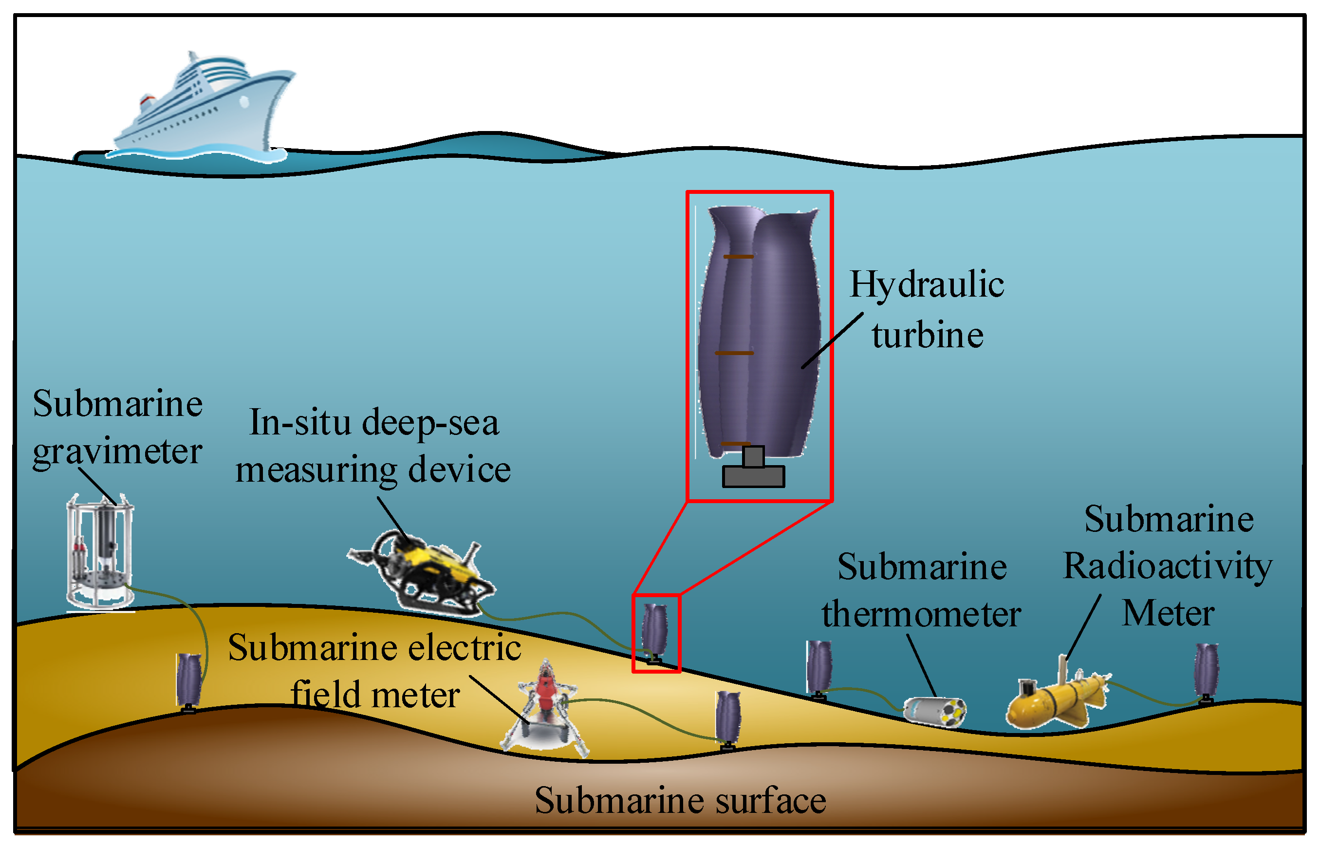
Deep-sea observation plays a crucial role in marine science and relies on a variety of geophysical instruments, such as submarine gravimeters, electric field meters, thermometers, and radioactivity meters, to assess key parameters, as shown in Figure 1. While progress has been made in short-term deep-sea observations, maintaining continuous operation of observation equipment for over a year remains a significant challenge, primarily due to power supply limitations. Ocean current energy offers a promising and sustainable energy source for deep-sea power solutions. Hydraulic turbines, the primary devices for harnessing ocean current energy, are ideal for deep-sea observation due to their minimal maintenance requirements and high reliability [1]. However, the slow flow speed of deep-sea currents prevents rotors from generating sufficient startup torque for continuous operation. Additionally, the high resistance, salinity, and pressure in deep-sea environments further hinder rotor startup. Therefore, understanding the startup process of the turbine rotor in low-speed ocean currents is crucial for enhancing its startup performance. To achieve this, tulip-type turbines are placed on the seabed to provide long-term, stable power for deep-sea observation instruments operating under challenging environmental conditions.

Hydraulic turbines are categorized into horizontal-axis and vertical-axis types [1]. A horizontal-axis turbine operates in a specific flow direction, while a vertical-axis turbine is effective in all flow directions [2]. Vertical-axis turbines are further classified as either drag-type or lift-type [3]. Various rotor configurations with different blade types exist for vertical-axis turbines. The S-type hydraulic turbine, a common drag-type vertical-axis turbine [4], exhibits excellent self-starting ability at low flow speeds, making it suitable for low-power applications [5,6,7,8,9]. However, its efficiency is limited by high drag during rotation. Various studies have examined performance improvements by modifying blade profiles [10,11,12,13], overlap ratios [14,15,16], aspect ratios [17], and inlet flow velocities [18].

Lift-type turbines, such as the D-type [19] and H-type [20] designs, typically achieve higher power coefficients but often exhibit poor self-starting performance [21,22]. To overcome this limitation, researchers have proposed blade shape optimization [23,24], hybrid S-D [25] or H-S [26] rotor designs, and flow concentrators [27] to improve startup behavior while preserving efficiency [28]. Novel geometries, such as helical blades [29], have also been introduced to stabilize torque generation and enhance power output [30,31].

Inspired by these developments, the tulip-type turbine, a novel form of drag-type turbine, is gradually attracting the attention of researchers. Its blade shape resembles that of a tulip flower, as shown in Figure 2. Unlike the traditional S-type rotor, the tulip-type rotor has two main differences: first, it has a bulbous structure with the widest section at the middle, and second, it features an expanded opening at the top. Paul et al. [32] and Kanthaiah et al. [33] studied the design and fabrication of tulip-type wind turbines, emphasizing their potential for clean energy generation with minimal environmental impact. They suggest that the tulip-type turbine design enhances torque generation, potentially resulting in a higher power coefficient than conventional vertical-axis rotors. Its compact structure, stability, turbulence adaptability, low noise, reduced flow requirements, safety, ease of maintenance, aesthetic appeal, and modular scalability make it particularly suitable for deep-sea applications.

In deep-sea environments, turbines face unique challenges, including limited maintenance access, persistently low current velocities, high salinity, elevated hydrostatic pressure, and complex unsteady flow conditions. The bulbous structure and expanded top opening of the tulip-type design may enhance flow capture and torque generation under weak currents, while its stable drag-based configuration enables reliable self-starting, essential for long-term unattended underwater operations. Despite these advantages, detailed studies on the hydrodynamic performance and startup mechanisms of tulip-type turbines in underwater applications remain limited.

The literature review indicates that while the flow field and startup performance of many common blade-type rotors have been extensively studied, the performance of the tulip-type hydraulic turbine rotor, with its innovative design, remains insufficiently understood. This study aims to systematically investigate the startup mechanism of tulip-type rotors and assess their potential for deep-sea applications. The CFD method is employed to numerically solve the problem. The self-rotation process of the rotor driven by the flow is solved using a six degrees of freedom (SDOF) solver. Typical flow patterns and vortex behaviors around and downstream of the rotor are presented. The flow characteristics near the expanded top design of the tulip-type rotor are described, highlighting the role of this feature. The model results are validated by comparison with experimental data. The unique flow field and vortex patterns of the tulip-type rotor are examined to clarify its startup mechanism. This research provides valuable insights into optimizing the performance and efficiency of tulip-type turbines, which could enhance their practical application in renewable energy systems.

2. Methodology

2.1. Problem Description of the Tulip-Type Turbine Rotor

The present prototype tulip rotor geometry is shown in Figure 3a. The turbine rotor has two tulip-shaped blades with the same height H that are rotationally symmetrical with respect to the y-axis. Four cross-sections, labeled p₁, p₂, p₃, and p₄ from top to bottom, depict the main shape of the tulip rotor in the x-z plane. The blade shape transitions from expanding at p₁ to shrinking at p₂, then expanding significantly to the largest tulip blade profile at p₃, and finally shrinking again at p₄. The blade shapes at these cross-sectional planes are illustrated in Figure 3b. Plane p₃ features a bulbous structure at the maximum radius, with narrowing on both sides at p₂ and p₄. Unlike the S-type rotor, the rotor blade profile at p₃, as shown in Figure 3b, is not semicircular but resembles a segment of an Archimedean spiral. At p₁, the top expands outward. The curves at p₁, p₂, p₃, and p₄ form the complete tulip blade rotor through the lofting function in geometry-modeling software. The extent of blade overlap is defined by the distance e, as shown in Figure 3c. The rotor diameter, D, is defined as the distance between the outer edges of the largest tulip blade profile in the top view. The azimuthal angle, θ, is defined as the angle between the line connecting the two blade tips and the opposite direction of the inlet flow. The velocity of the inlet flow, U, remains constant as the rotor rotates.

2.2. Equations of CFD Modeling

This study uses the Computational Fluid Dynamics (CFD) method to solve the flow around the turbine rotor, enabling evaluation of the rotor’s performance. The mass conservation equation, momentum equations, turbulence equations, and equations describing the rotor characteristics are then presented.

2.2.1. Mass Conservation and Momentum Equations

The mass conservation equation (see Equation (1)) ensures the continuity of mass flow in the system and is essential for analyzing the flow behavior around the tulip-type rotor:

$${\displaystyle \frac{\mathsf{\partial }}{\mathsf{\partial }{x}_i}}\left({\overline{u}}_i+u_i^{\prime }\right)=0$$

(1)

where ${\overline{u}}_i$ denotes the average flow velocity, $u_i^{\prime }$ indicates the velocity fluctuation due to turbulence, and x represents the flow direction.

The momentum equation (see Equation (2)) governs the forces acting on the fluid and is crucial for understanding the fluid dynamics and rotor performance in this study. It is solved in conjunction with the mass conservation equation.

$${\displaystyle \frac{\mathsf{\partial }{\overline{u}}_i}{\mathsf{\partial }t}}+{\overline{u}}_j{\displaystyle \frac{\mathsf{\partial }{\overline{u}}_i}{\mathsf{\partial }{x}_j}}=-{\displaystyle \frac{1}{\rho }}{\displaystyle \frac{\mathsf{\partial }\overline{p}}{\mathsf{\partial }{x}_i}}+{\displaystyle \frac{\mu }{\rho }}{\displaystyle \frac{{\mathsf{\partial }}^2{\overline{u}}_i}{\mathsf{\partial }{x}_j\mathsf{\partial }{x}_j}}-{\displaystyle \frac{\mathsf{\partial }}{\mathsf{\partial }{x}_j}}\overline{u_i^{\prime }{u}_j^{\prime }}$$

(2)

where t is time, $\overline{p}$ is the average pressure, $\rho$ is the density, and $\mu$ is the dynamic viscosity of the flow.

2.2.2. Turbulence Equations

From Equation (2), the term $\rho \overline{u_i^{\prime }{u}_j^{\prime }}$ arises, representing the Reynolds stress tensor, which introduces six additional unknowns. To address the closure problem caused by these additional terms, the turbulence equations (Equations (3)–(5)) are solved:

$$\begin{array}{l}{\displaystyle \frac{\mathrm{d}}{\mathrm{d}t}}{\displaystyle \underset{V}{\int }\rho k\mathrm{dV}+}{\displaystyle \underset{A}{\int }\rho k}\left(\mathit{v}-{\mathit{v}}_{\mathbf{g}}\right)\cdot \mathrm{d}\mathit{a}={\displaystyle \underset{A}{\int }\left(\mu +{\sigma }_{\mathrm{k}}{\mu }_{\mathrm{t}}\right)}\nabla k\cdot \mathrm{d}\mathit{a}+{\displaystyle \underset{V}{\int }\left({\gamma }_{\mathrm{eff}}{G}_{\mathrm{k}}\right.}-{\gamma }^{\prime }\rho {\beta }^{*}{f}_{\mathsf{\beta }}\left({\omega }_{\mathrm{t}}k-{\omega }_{\mathrm{t}0}{k}_0\right)+\left.S_k\right)\mathrm{dV}\end{array}$$

(3)

$$\begin{array}{l}{\displaystyle \frac{\mathrm{d}}{\mathrm{d}t}}{\displaystyle \underset{V}{\int }\rho {\omega }_{\mathrm{t}}\mathrm{dV}+}{\displaystyle \underset{A}{\int }\rho {\omega }_{\mathrm{t}}}\left(\mathit{v}-{\mathit{v}}_{\mathbf{g}}\right)\cdot \mathrm{d}\mathit{a}={\displaystyle \underset{A}{\int }\left(\mu +{\sigma }_{{\omega }_{\mathrm{t}}}{\mu }_{\mathrm{t}}\right)}\nabla {\omega }_{\mathrm{t}}\cdot \mathrm{d}\mathit{a}+{\displaystyle \underset{V}{\int }\left(G_{{\omega }_{\mathrm{t}}}\right.}-\rho \beta f_{\mathsf{\beta }}\left({\omega }_{\mathrm{t}}^2-{\omega }_{\mathrm{t}0}^2\right)+\left.D_{{\omega }_{\mathrm{t}}}+S_{{\omega }_{\mathrm{t}}}\right)\mathrm{dV}\end{array}$$

(4)

$${\gamma }^{\prime }=\min \left[\max \left({\gamma }_{\mathrm{eff}}\prime 0.1\right)\prime 1\right]$$

(5)

where k is the turbulent kinetic energy, ${\omega }_{\mathrm{t}}$ is specific dissipation rate, V is the cell volume, A is the area, a is the face area vector, v is the flow velocity, and v_g is the velocity of the grid. ${\sigma }_k$ and ${\sigma }_{{\omega }_{\mathrm{t}}}$ are the inverse turbulent Schmidt numbers, and ${\mu }_{\mathrm{t}}$ is the turbulent viscosity. $S_k$ and $S_{{\omega }_{\mathrm{t}}}$ are user-defined source terms, while $k_0$ and ${\omega }_{\mathrm{t}0}$ represent ambient turbulence values included in source terms to counteract turbulence decay. ${\gamma }_{\mathrm{eff}}$ denotes the effective intermittency, and $D_{{\omega }_{\mathrm{t}}}$ is a cross-derivative term defined by Equation (6).

$$D_{{\omega }_{\mathrm{t}}}=2\left(1-F_1\right)\rho {\sigma }_{{\omega }_{\mathrm{t}}2}{\displaystyle \frac{1}{{\omega }_{\mathrm{t}}}}\nabla k\cdot \nabla {\omega }_{\mathrm{t}}$$

(6)

where F₁ is the blending function. The turbulent viscosity ${\mu }_{\mathrm{t}}$ are derived from solutions of Equations (3) and (4), which is given by Equation (7) and relates to the Reynolds stress tensor $\rho \overline{u_i^{\prime }{u}_j^{\prime }}$ through Equation (8), thereby solving the closure problem.

$${\mu }_{\mathrm{t}}=\rho k{\mathrm{T}}_{k{\omega }_{\mathrm{t}}}$$

(7)

$$-\rho \overline{u_i^{\prime }{u}_j^{\prime }}={\mu }_t\left({\displaystyle \frac{\mathsf{\partial }{\overline{u}}_i}{\mathsf{\partial }{x}_j}}+{\displaystyle \frac{\mathsf{\partial }{\overline{u}}_j}{\mathsf{\partial }{x}_i}}\right)-{\displaystyle \frac{2}{3}}\rho k{\delta }_{ij}$$

(8)

where ${\delta }_{\mathrm{ij}}$ denotes the Kronecker delta operator.

2.2.3. Rotor’s Characteristics

According to Newton’s second law of motion, the rotor’s rotational velocity ω is influenced by multiple factors, including the moment of inertia J, the hydraulic moment T_w, the frictional resistance moment T_r, and the external load moment T_l. The hydraulic rotor rotates about its central axis, and its rotational dynamics are governed by the following equation:

$$J{\displaystyle \frac{\mathrm{d}\omega }{\mathrm{d}t}}=T_{\mathrm{w}}-T_{\mathrm{r}}-T_{\mathrm{l}}$$

(9)

where t is time. Integrating Equation (9) yields the rotor’s rotational velocity ω:

$$\omega ={\displaystyle \int \frac{T_{\mathrm{w}}-T_{\mathrm{r}}-T_{\mathrm{l}}}{J}}\mathrm{d}t$$

(10)

The moment of inertia J depends on the rotor’s geometry, material, and its connection to the adjacent module. The hydraulic moment T_w is obtained by integrating the static pressure and shear stress over the rotor blade surface. Since the frictional resistance moment T_r has minimal impact on rotor rotation, it was excluded from this study. Likewise, the external load moment T_l was not considered, implying that the rotor is assumed to operate under a no-preload condition.

The tip-speed ratio (TSR) is defined as the ratio of the rotor’s maximum linear velocity at the blade tip to the upstream flow velocity U:

$$TSR={\displaystyle \frac{\omega D}{2U}}$$

(11)

2.3. Numerical Setup

The numerical simulation utilized the commercial CFD software ANSYS Fluent 19.2. The entire numerical domain is governed by the Reynolds-averaged Navier-Stokes (RANS) equations. To simultaneously solve the momentum and continuity equations, the SIMPLE pressure–velocity coupling solver was used. Convective terms in the governing equations were discretized using a second-order upwind scheme, selected for its reduced dependence on grid refinement and its ability to avoid pseudo-diffusion compared to a first-order scheme. The shear stress transport (SST) k-ω turbulence model was employed, combining the advantages of the standard k-ε and k-ω models, making it suitable for flows near rotating blades [31]. Additional details about the SST k-ω turbulence model are available in references [34,35]. All simulations were conducted with convergence criteria set to 1 × 10⁻⁶ for the entire computational domain.

A six-degree-of-freedom (SDOF) solver is incorporated for simulating the flow-driven rotation of the rotor [36]. The computational domain for the tulip rotor is shown in Figure 4, consisting of a rotational subdomain and an outer domain. In the streamwise (negative z) direction, the inlet and outlet of the entire domain are located 5D upstream and downstream from the rotor axis, respectively. In the y-direction, the top and bottom boundaries are positioned 2.5D from the rotor center. In the x-direction, the front and back boundaries are set 1.1D from the rotor center. The computational domain is designed to be sufficiently large to prevent boundary disturbances from affecting the flows near the rotor, ensuring fully developed inflow to the rotor and accurate capture of wake vortex phenomena. Interfaces between adjacent subdomains are defined to ensure reliable data exchange and conservation of mass and momentum.

The boundary conditions for the computational domain are defined as follows: a uniform upstream velocity is imposed at the inlet, and a constant pressure is set at the outlet. Symmetry boundary conditions are applied to the top and bottom boundaries (in the y-direction) and the front and back boundaries (in the x-direction). A no-slip condition is enforced on the rotor blade surfaces. Due to numerical limitations, deep-sea high-pressure conditions were not considered.

An unstructured tetrahedral grid is chosen for its minimal truncation errors and convergence efficiency. The commercial grid generation software ICEM CFD is used to discretize the computational domain. Figure 5 presents the cross-sectional grid distribution on plane p₃ of the rotor (see Figure 3). The thickness of the initial layer of cells adjacent to the blade surface is set to 0.001 m, with a total of six near-wall layers exhibiting a growth ratio of 1.2. Grid refinement is concentrated near the blade surface. The sliding mesh technique is applied at the interfaces between adjacent subdomains to ensure accurate data exchange during rotor rotation [37].

To evaluate the numerical solution’s convergence, a mesh convergence check was conducted using an inlet flow velocity of U = 4 m/s. Figure 6 presents the variation in the average torque coefficient ${\overline{C}}_{\mathrm{t}}$ with mesh number. The value ${\overline{C}}_{\mathrm{t}}$ is obtained by time-averaging the torque coefficient C_t, which quantifies the turbine’s torque in relation to fluid dynamics, providing insights into its efficiency and torque output under specific conditions [38], with the equation as follows:

$$C_{\mathrm{t}}={\displaystyle \frac{2T}{0.5\rho A{U}^{2}D}}$$

(12)

where T represents the torque generated by the turbine, ρ is the fluid density, and A denotes the upstream-facing area of the rotor. As shown in Figure 6, ${\overline{C}}_{\mathrm{t}}$ stabilizes at 0.048 as the mesh number increases to 1.26 million. Further increasing the mesh number from 1.26 million to 4.25 million results in only an 8.2% reduction in ${\overline{C}}_{\mathrm{t}}$, while the computational time extends from approximately one week to three weeks. Considering the balance between accuracy and computational cost, the numerical solution’s convergence with the current model is deemed satisfactory. Therefore, the final grid scheme for the rotor consists of 1.26 million elements.

2.4. Validation of the Numerical Scheme

This section describes the experimental setup and validates the numerical results by comparing them with experimental data.

2.4.1. Experimental Setup

The experiments were conducted in the Marine Geophysical Exploration Simulation Laboratory at the School of Geophysics and Information Technology, China University of Geosciences (Beijing). Figure 7a,b show the water tank test system and its schematic representation. As illustrated in Figure 7a, the rotor is positioned inside a circulating open-water tank measuring 5 m in length, 2.5 m in effective width, and 1.8 m in height. Water circulation is maintained through three longitudinally arranged tubes connected to a centrifugal pump with a power rating of 2.2 kW and a flow capacity of 44.7 m³/h. To measure U at various upstream positions relative to the rotor, a propeller-type flow meter (LS20B) is mounted on a movable base, allowing both horizontal and vertical adjustments, as shown in Figure 7a. Throughout all flow conditions, the rotor remains fully submerged.

Figure 8a shows the experimental setup with a tulip-type rotor. The turbine blades, made of composite material, have a thickness of 2.5 mm and a height of 0.68 m. These blades are attached to a rotor shaft with a diameter of 25 mm. The upper end of the rotor shaft is connected to a high-precision dynamic torque sensor (STBD TorqSense S2104) via a coupling, enabling real-time measurement of the rotor’s torque and rotational speed, as illustrated in Figure 8a. To apply an external load, an electromagnetic powder brake (Magtrol CZ-500, Beijing Tianyu Hengchuang Sensing Technology Co., Ltd., Beijing, China) is mounted at the top of the dynamic torque sensor. The load applied to the rotor is precisely regulated by adjusting the DC current supplied to the magnetic powder brake, enabling accurate control of the braking force.

To measure the incoming flow velocity U at the rotor’s position, the flow meter is installed in place of the blades on the rotor shaft, as shown in Figure 8b. Vertical velocity measurements are taken at eight distinct positions along the rotor shaft, with data recorded at each location (marked by red solid circles in Figure 8b). The final incoming flow velocity U is determined as the average of these measurements.

Table 1. Summary of key measuring equipment and specifications.

Equipment	Model	Measurement Range	Measurement Error
Flow velocity meter	LS20B Propeller-type	0.04–15 m/s	≤1.5%
Torque sensor	STBD TorqSense S2104	0–500 Nm	0.1% F.S.
Electromagnetic powder brake	Magtrol CZ-500	0–500 Nm (braking)	N/A
Circulating pump	65-100IA-2.2	0–44.7 m3/h	N/A

summarizes the measuring equipment used in the experimental setup, including their models, measurement ranges, and errors, providing an overview of the measurement system for experimental validation.

2.4.2. Validation Results

Experiments were conducted using the same geometric and operational parameters as the numerical simulations (U = 4 m/s) to validate the present model. Figure 9 compares the numerical and experimental results for the rotor’s ${\overline{C}}_{\mathrm{t}}$ and ${\overline{C}}_{\mathrm{p}}$. The value ${\overline{C}}_{\mathrm{p}}$ is obtained by time-averaging the power coefficient C_p, which quantifies the turbine’s efficiency in converting the flow kinetic energy into mechanical energy, representing the ratio of generated mechanical power to the fluid dynamic power [39] as follows:

$$C_{\mathrm{P}}={\displaystyle \frac{\omega T}{0.5\rho A{U}^3}}$$

(13)

As shown in Figure 9, the numerical results exhibit a similar trend to the experimental data for both ${\overline{C}}_{\mathrm{t}}$ and ${\overline{C}}_{\mathrm{p}}$, though the experimental values are consistently higher. This discrepancy can be attributed to two primary factors: (1) numerical dissipation, caused by mesh resolution limitations and turbulence modeling, which may lead to artificial energy loss during simulation; and (2) the lack of the central shaft between the two blades in the numerical rotor model. Despite these differences, the validation confirms that the flow physics in the current simulations are reasonably well captured.

3. Results and Discussion

In this section, typical flow patterns and vortices around the rotor are presented numerically, and their effects on the rotor’s startup performance are discussed. The values of rotor parameters used in the numerical simulations are summarized in

Table 2. Values of the turbine rotor parameters for numerical analysis.

Parameters	Value
D (m)	0.32
H (m)	0.68
e (m)	0.08
θ (°)	90
m (kg)	1.3
U (m/s)	0.25, 0.5, 1, 2, 3, 4, 5, 6

. The moment of inertia around the y-axis was J = 0.0224 kg·m² based on the rotor’s geometry and material density. Pure water at 20 °C, with a density of 998.2 kg/m³ and dynamic viscosity of 1.0 × 10⁻³ Pa·s, was selected as the incompressible working fluid. The numerical simulation begins with the rotor at rest, starting from an azimuthal angle of θ = 90° (see Figure 3).

In this study, numerical investigations were conducted across a range of inlet velocities, U, from 0.25 to 6 m/s to examine their effects on turbine rotor performance. The torque coefficient C_t and power coefficient C_p were calculated for each case. The highest C_t and C_p values were observed at around 4 m/s, indicating optimal startup performance and energy conversion efficiency. Therefore, U = 4 m/s was selected as the reference case for the detailed analysis of transient flow patterns and vortex evolution presented in this paper.

3.1. Typical Flow Pattern

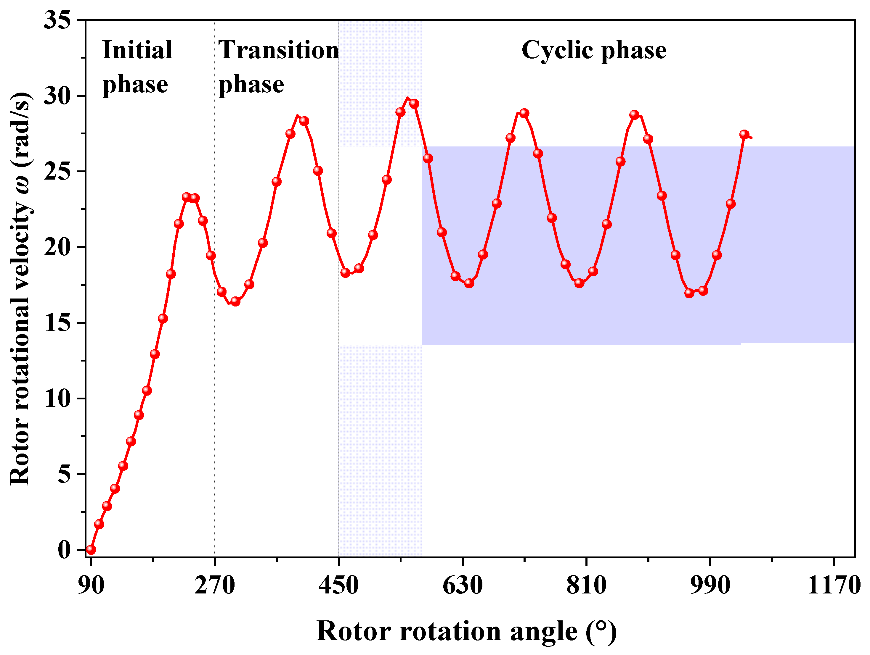
Figure 10 shows a typical variation in the rotor’s rotational velocity, ω, with the rotor’s rotation angle, which starts from θ = 90° under an inlet velocity of U = 4 m/s. The rotational velocity exhibits three distinct phases during the rotor’s rotation: initial, transition, and cyclic phases. The startup process includes the initial and transition phases. The initial phase covers the first half-turn (from θ = 90° to 270°), during which the rotational velocity increases and then decreases. The transition phase occurs during the second half-turn (from θ = 270° to 450°), where the rotational velocity approaches oscillation. After the transition phase, the rotor enters a stable, cyclic phase of rotational velocity. Successful rotor startup is defined as completing a full rotation of 360° (from θ = 90° to 450°). The present study focuses on the rotor’s startup process, particularly the initial and transition phases.

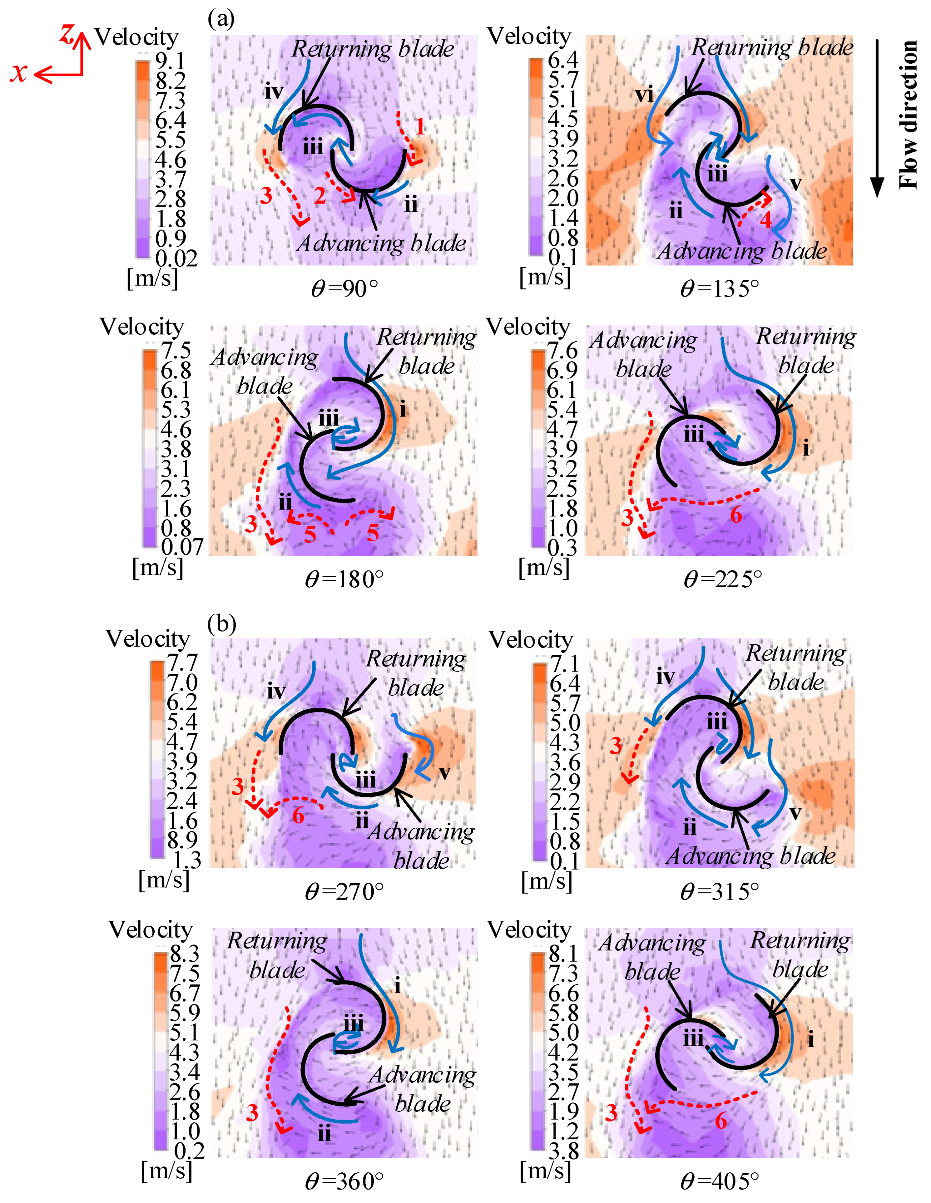
Figure 11 illustrates the flow results within tulip rotors at a reference velocity of U = 4 m/s, starting from θ = 90° on plane p₃ (see Figure 3). This plane is highlighted because it passes through the maximum diameter region of the tulip-type rotor, which is crucial for capturing hydrodynamic energy. The flow patterns during the initial and transition phases are shown in Figure 11a and Figure 11b, respectively. The color map in Figure 11 indicates the flow velocity magnitude, with warmer colors representing higher velocities and cooler colors representing lower velocities. The arrows on the flow pattern illustrate the direction of flow, showing the velocity vectors at each point in the field. The Roman numerals (i) to (vi) represent flow patterns common to both the novel tulip and traditional S-type rotors, indicated by blue solid curves with arrows. The Arabic numerals (1) to (6) represent unique flow patterns occurring only in the tulip-type rotor, marked by red dashed curves with arrows. These flow patterns are described as follows, with their corresponding numerals in Figure 11a,b:

(i)

Attached flow along the returning blade’s convex side.

(ii)

Dragging flow from the advancing blade’s convex surface to the returning blade’s concave side.

(iii)

Through-flow in the overlapping area.

(iv)

Flow from upstream of the rotor to the returning blade’s convex side.

(v)

Shedding vortex from the advancing blade’s tip.

(vi)

Shedding vortex from the returning blade’s tip.

These flow patterns are similar to those observed around a standard S-type rotor in ref. [7], because the tulip-type blades share a basically similar geometry with the S-type, despite differences in specific blade shapes. In addition to these common flow patterns, unique flow features of the tulip rotor are found and described below.

During the initial phase (from θ = 90° to 225°), as shown in Figure 11a, the upstream flow moves in the negative z-direction. As the rotor starts rotating from θ = 90°, a high-speed flow passes the tip of the advancing blade, labeled as (1). In contrast, in the S-type rotor, the shedding vortex (flow v) occurs at this position. The absence of this shedding vortex in the tulip rotor at this stage likely results from incomplete vortex development near the blade tip at the onset of rotation.

A second unique phenomenon observed in the tulip rotor, marked as (2), is a return flow from the concave side of the returning blade toward the convex surface of the advancing blade. This return flow occurs because the dragging flow (ii) lacks sufficient momentum to continue smoothly from the advancing blade’s convex side to the returning blade’s concave side.

Additionally, an upstream flow moves along the convex side of the returning blade and directly away from its tip, labeled as (3). In contrast, the S-type rotor typically exhibits the shedding vortex (flow vi) at the returning blade’s tip. The absence of vortex shedding at this location in the tulip-type rotor is due to its bulbous, widest midsection (see Figure 3b), which smooths the flow path and prevents vortex formation near the blade tip.

At θ = 135°, another distinct flow characteristic emerges: a return flow from the convex surface of the advancing blade toward its tip, labeled as (4). This return flow is caused by the large vortex covering nearly half of the convex surface area of the advancing blade (see Figure 12).

At θ = 180°, two additional flow features are observed. First, a pair of opposing flows, labeled as (5), emerges behind the rotor due to the formation of counter-rotating vortices in this region (see Figure 12). Second, flow (3) continues to develop as upstream fluid moves along the convex surface of the advancing blade and away from its tip. The flow (3) maintains till θ = 225°, at which point the tulip-type rotor still does not exhibit the blade-tip vortex (flow v in S-type rotor). Moreover, at this angle, a transverse flow appears in the x-direction from the trailing edge of the returning blade toward the tip of the advancing blade, labeled as (6).

Figure 11b illustrates the subsequent transition phase (from θ = 270° to 405°), beginning when the rotor reaches θ = 270°. At θ = 270°, the transverse flow (6) in the x-direction near the trailing edge of the advancing blade merges with the continuing flow (3). Flow (3) remains clearly identifiable at θ = 315°. By θ = 360°, the attached flow continues along the advancing blade’s convex surface and subsequently moves outward from its tip, again identified as flow (3). The transverse flow (6) also remains observable at θ = 405°. After the transition phase, the flow stabilizes into a cyclic phase, characterized by repetitive and consistent hydrodynamic behavior. This cyclic phase maintains the flow features established during the latter half of the transition phase (θ = 270° to 450°).

3.2. Vortex near Rotor

The startup performance of the rotor is significantly influenced by the surrounding vortex structures. Analyzing the evolution of these vortices helps clarify their effects on blade drag and thrust during the startup phase. Figure 12 illustrates pressure distributions and velocity vectors on the top plane p₁, middle plane p₃, and bottom plane p₄ during the initial phase. The color contours indicate pressure magnitude, with red representing high-pressure regions and blue representing low-pressure regions. The arrows overlaying the contours depict local flow directions. Vortices positively contributing to rotational moment generation are indicated by red solid arrows, whereas vortices negatively affecting rotational moment generation are shown by blue dashed arrows.

At θ = 135°, a pair of counter-rotating vortices forms near the convex side of the advancing blade on plane p₁, creating low-pressure regions that enhance positive (clockwise) moment generation. On planes p₃ and p₄, a small vortex emerges within the blade-overlap region, corresponding to flow (iii) in Figure 11. This vortex reduces local pressure, thereby weakening the positive moment for both blades.

Additionally, a vortex near the tip of the advancing blade appears on planes p₃ and p₄, lowering pressure on the convex surface and thus aiding positive moment generation; this vortex corresponds to flows (v) and (4) in Figure 11. Meanwhile, on plane p₃, another vortex forms near the tip of the returning blade’s concave side, creating a low-pressure area that negatively affects moment generation. This vortex corresponds to flow (vi) in Figure 11.

At θ = 180°, the vortex structures continue to evolve. On plane p₁, a negative vortex appears in the blade-overlap area. On planes p₃ and p₄, the vortex near the tip of the advancing blade remains but splits into two distinct vortices, corresponding to flow (5) in Figure 11. Meanwhile, the negative vortex near the returning blade’s tip disappears from plane p₃ but appears instead on plane p₄. At θ = 225°, the negative vortex within the blade-overlap region expands considerably on planes p₁ and p₄. On plane p₄, the negative vortex previously present near the returning blade’s tip disappears, indicating further redistribution of vortex structures.

At θ = 270°, on planes p₁ and p₄, a vortex near the advancing blade’s tip generates a notable low-pressure area that extends from the concave side of the advancing blade toward the convex side of the returning blade. This extended low-pressure area benefits positive moment generation of the returning blade. However, it negatively affects the advancing blade by increasing local drag, thereby reducing its positive moment generation.

In summary, the transient vortex evolution from θ = 135° to θ = 270° exhibits a systematic development and redistribution of vortices driven by blade geometry and local flow interactions. Initially isolated vortices merge or dissipate over time, significantly altering the pressure distribution on the blades and downstream regions. This evolving vortex structure directly impacts the thrust and drag characteristics during startup, highlighting the importance of blade geometry in optimizing transient hydrodynamic performance.

Figure 13 illustrates the pressure distribution and velocity vectors on planes p₁, p₃, and p₄ during the transition phase. At θ = 315°, the low-pressure area caused by the “negative” vortex in the overlapping area grows significantly compared to θ = 270°, while the vortex near the advancing blade’s tip disappears. The vortex near the tip of the returning blade reappears on planes p₁, p₃, and p₄, resulting in the flow (v) in Figure 11. This increases the area of low pressure on the convex side of the returning blade, benefiting the generation of positive moment for the rotor. On plane p₄, the vortex near the advancing blade’s tip at θ = 270° shifts now toward the convex side of the returning blade, further enhancing positive moment generation. At θ = 360° and 405°, the vortex near the returning blade’s tip disappears on planes p₁, p₃, and p₄, but the “negative” vortex in the overlapping area persists. At θ = 450°, a “positive” vortex reappears near the returning blade’s tip on plane p₄. After the transition phase, the vortex structures enter a cyclic state.

Overall, the evolution of the surrounding vortices primarily influences the generation of the rotor’s positive moment. During the initial and transition phases, the “positive” vortices on the blade’s convex side contribute beneficially, while the “negative” vortices on the blade’s concave side and in the overlapping region hinder positive moment generation. The counteracting effects of the “positive” and “negative” vortices affect the rotor’s startup performance. During the startup process, when the effect of the “positive” vortices outweighs that of the “negative” vortices, the rotor’s positive moment exceeds the negative moment, enabling successful startup.

3.3. Downstream Flow Field of the Rotor

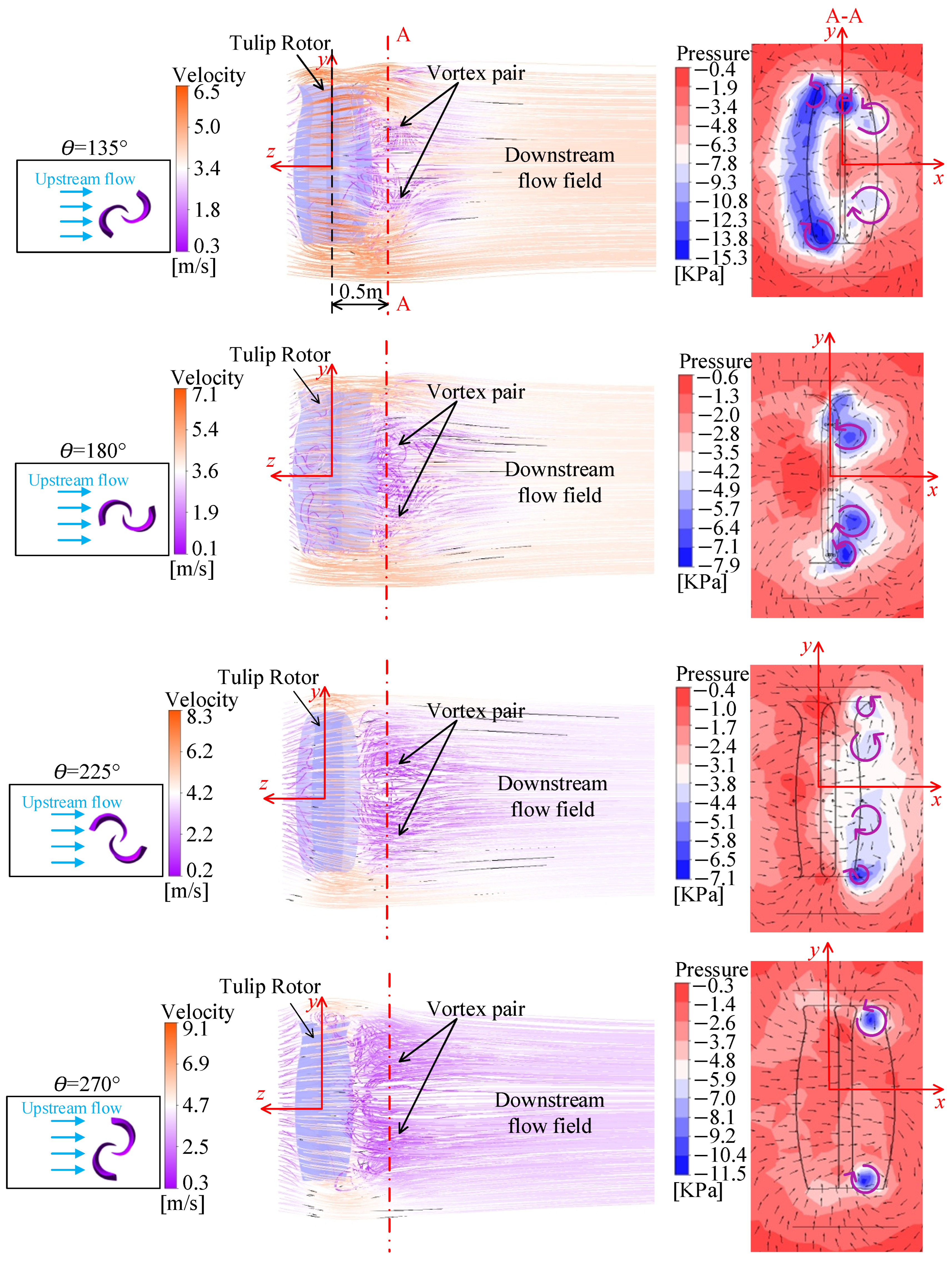
The flow field and vortex structures downstream of the rotor influence its moment output, thereby affecting startup performance and energy conversion efficiency. Figure 14 shows streamline distributions on the y-z plane and pressure distributions with velocity vectors on the longitudinal x-y cross-section A-A (marked by the dash-dot line), located 0.5 m downstream of the rotor from the y-axis, at θ = 135°, 180°, 225°, and 270° during the initial phase.

At θ = 135°, a pair of longitudinal vortices forms downstream of the rotor on both sides of the y = 0 plane (in the x-y plane), located at the upper and lower regions. These vortices form within the concave zones above and below the rotor’s widest midsection, where the bulbous tulip-shaped profile enhances local flow separation. The intensity of these vortices gradually decreases downstream along the negative z-direction. In contrast, an S-type rotor typically generates a single vortex structure on the x-z plane due to its uniform geometry along the rotor height (y-direction). The intensity of this vortex also gradually decreases downstream in the negative z-direction, forming a pattern similar to a classical Karman vortex street. From cross-section A-A at θ = 135°, two vortices appear in the upper region, while another low-pressure vortex forms in the lower region near the rotor’s central axis (close to the x = 0 plane).

At θ = 180°, the downstream vortex pair shifts slightly toward the rotor’s widest midsection and intensifies. In the A-A cross-section, the upper vortices vanish, while the lower one shifts toward the positive x-direction and reverses its rotational direction compared to that at θ = 135°. At θ = 225°, the vortices on the y-z plane grow larger and more distinct, extending farther downstream, as indicated by the increased velocity magnitudes in Figure 14. This reflects intensified vortex dynamics and stronger interaction with the main flow. In the A-A cross-section, two vortex pairs emerge symmetrically on either side of the y = 0 plane: both the larger and smaller pairs rotate in opposite directions to each other.

At θ = 270°, the streamline pattern becomes denser and more disordered, with higher velocities indicated by the color scale. In the A-A cross-section, the central vortex pair disappears, leaving only a smaller vortex pair near the top and bottom of the rotor.

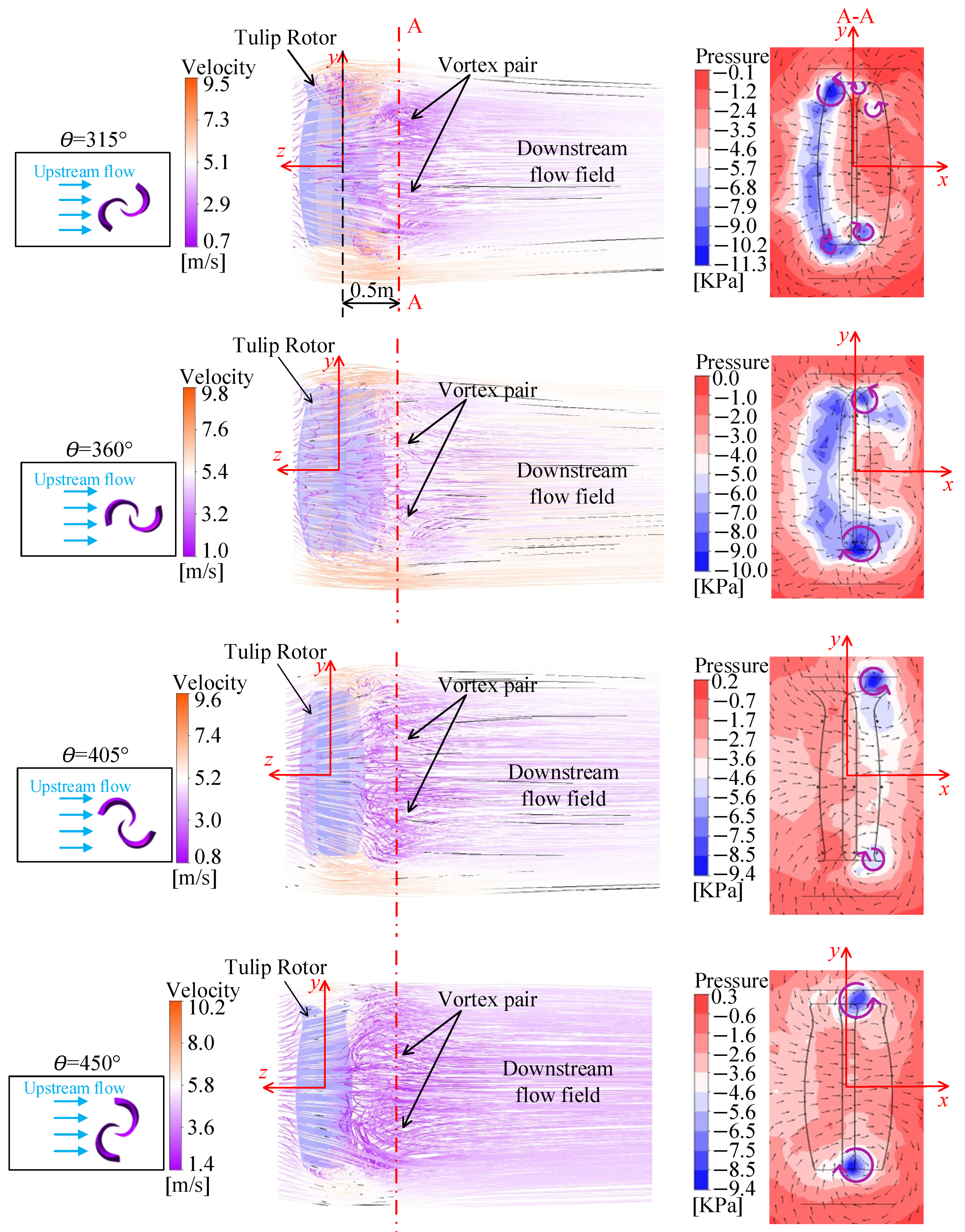
Figure 15 illustrates results during the transition phase at θ = 315°, 360°, 405°, and 450°. At θ = 315°, the increased rotational speed of the rotor relative to the initial phase further intensifies downstream vortices, expanding vortex regions along both y- and z-directions. Cross-section A-A indicates the formation of two additional vortices in the top region and one additional vortex in the bottom region. At this stage, the velocity and pressure magnitudes, as indicated by the color scale, significantly increase compared to earlier phases.

At θ = 360°, these multiple vortices merge into a single vortex in each of the top and bottom regions, with a clear increase in vortex intensity (reflected by elevated velocity and pressure magnitudes). As θ progresses to 405°, the vortices separate further from the widest midsection of the rotor. Subsequently, at θ = 450°, these vortices reconverge toward positions resembling those at θ = 360°, indicating the onset of periodic vortex behavior.

Overall, downstream vortices consistently form behind the convex surfaces of both advancing and returning blades, generating low-pressure zones. This enhances the pressure difference between concave and convex blade surfaces, contributing positively to the rotational moment, consistent with phenomena observed during the initial startup phase.

However, unlike the initial phase, the transition phase demonstrates a progressive increase in the intensity and redistribution of downstream vortices, approaching stable periodic flow structures as rotor speed increases. This stabilization is also reflected in the rotor’s speed curve (see Figure 10), where rotational velocity approaches cyclic steady-state behavior, distinguishing it from the early transient startup process.

Notably, at very high inflow velocities (high Reynolds numbers), downstream vortices intensify significantly, potentially resulting in highly turbulent flow conditions. Such turbulence may adversely affect rotor performance by increasing drag and disrupting smooth blade rotation.

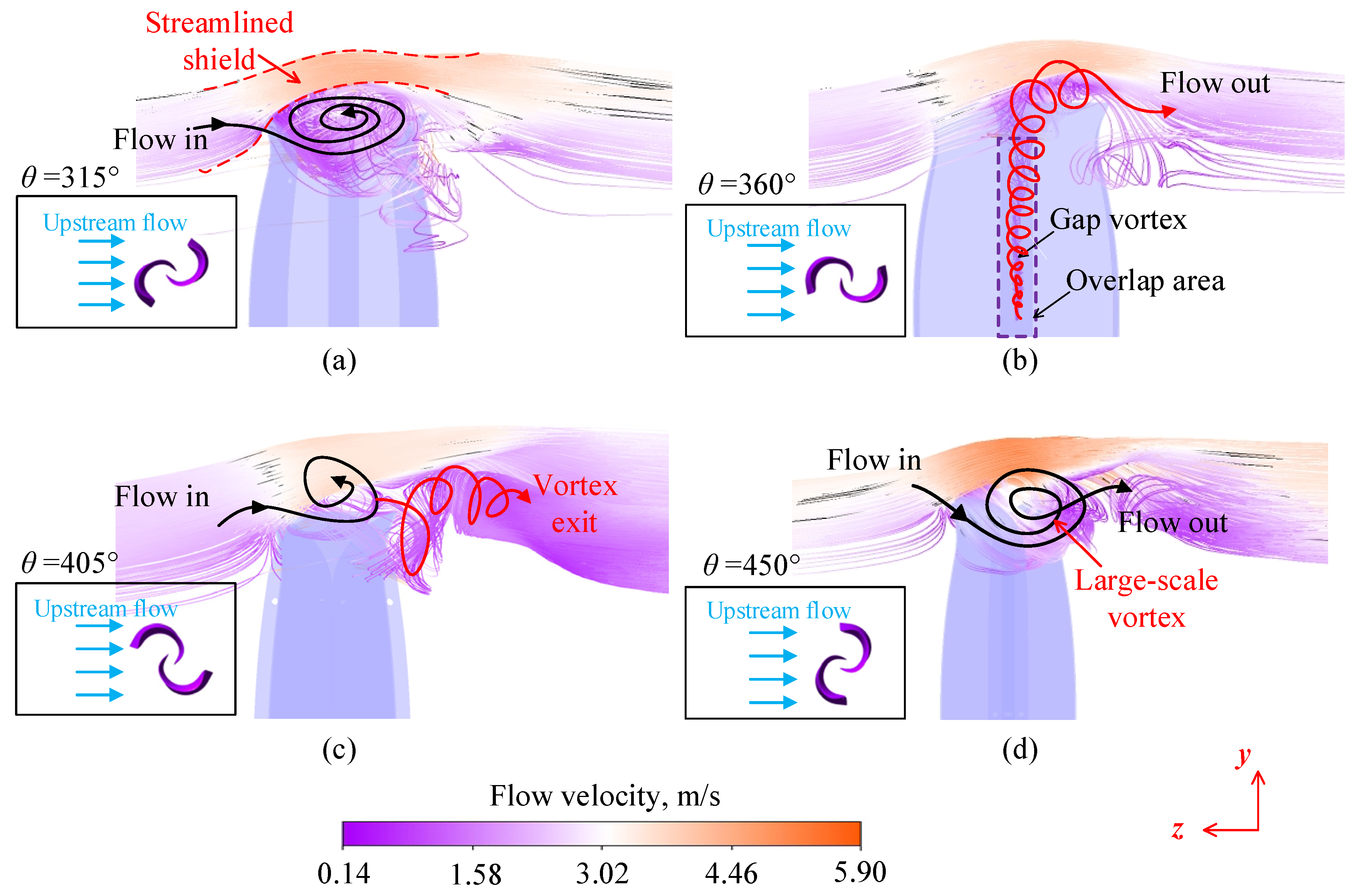
3.4. Streamlines at the Expanded Top of the Rotor

During the initial phase, the vortex at the expanded top of the rotor is not prominent, as illustrated in Figure 14. However, as the transition phase progresses, the vortex at the expanded top intensifies, as shown in Figure 15, highlighting the importance of the expanded top design. To clarify the role of this design, Figure 16a–d present the streamline distributions around the expanded top of the rotor at θ = 315°, 360°, 405°, and 450°, respectively. The colors in Figure 16 represent flow velocity magnitudes, with different colors indicating variations from low to high velocities.

At θ = 315°, the orange streamlines above the rotor flow smoothly from the inlet, forming a distinct flow-guiding layer like a shield. This layer effectively channels fluid around the horn-shaped opening of the expanded top, directing more flow into the blade’s working region and maximizing kinetic energy capture.

At θ = 360°, the slender gap vortices develop in the overlapping region between the two tulip blades. These vortices reduce the rotor’s rotational efficiency, as discussed in Section 3.2. The expanded top guides them outward along its surface, promoting their dissipation and minimizing their negative impact.

At θ = 405°, the expanded top primarily serves as a vortex-clearance passage, guiding vortices out of the rotor region and preventing clogging. This clearance reduces internal turbulence, maintains stable torque production, and decreases blade-induced vibration and operational noise.

At θ = 450°, the large-scale vortices form within the upper rotor region due to the expanded top. These vortices enhance fluid-blade interactions, significantly increasing momentum exchange and energy transfer efficiency. Consequently, this improves rotor torque and startup performance.

In summary, the expanded top design serves four distinct and clearly differentiated functions across these phases: flow guiding at θ = 315°, vortex dissipation at θ = 360°, vortex clearance at θ = 405°, and enhanced fluid-blade interaction at θ = 450°.

3.5. Summary of Flow and Vortex Distribution

Figure 17 summarizes the distinct flow patterns and vortex structures generated by the unique geometry of the tulip-type rotor. Flow paths are represented by black lines, while positive and negative vortices are shown by red solid and blue dashed lines, respectively.

At the expanded top, incoming fluid enters the enlarged region (a), forming large-scale vortices (b) smoothly guided outward through the horn-shaped opening. This expanded structure also effectively dissipates slender gap vortices spiraling upward from the rotor base, reducing their negative impact on rotor rotation (c).

In the middle region, characterized by an enlarged blade radius, upstream fluid closely follows the convex surfaces of both the advancing and returning blades. These streams then converge downstream (d), with some fluid moving from the convex side of the advancing blade into the concave side of the returning blade (e). Additionally, lateral flow occurs from the rear edge of the advancing blade toward the tip of the returning blade (f). Some upstream fluid directly enters the concave side of the advancing blade (g), further enhancing rotational momentum. A “positive” vortex develops near the outer tip of the advancing blade’s convex side (h), while a “negative” vortex emerges on the concave side of the returning blade (i). Downstream, two counter-rotating vortices form symmetrically in the upper and lower regions, rotating as they move downstream (j).

These fluid flows and vortex structures collectively clarify the startup mechanism of the tulip-type rotor, offering valuable insights into transient flow behavior and vortex evolution to support the optimization of hydraulic turbine performance.

3.6. Quantitative Analysis of Vortex Strength, Circulation, and Drag Coefficient

To further clarify the startup mechanism, quantitative analyses of vortex strength, circulation, and drag coefficient are performed based on the CFD results. Vortex strength is characterized by the vorticity magnitude, representing local rotational intensity. The vorticity vector ω is defined as follows:

$$\mathsf{\omega }=\nabla \times U$$

(14)

The vorticity magnitude is as follows:

$$\left|\omega \right|=\sqrt{{\omega }_x^2+{\omega }_y^2+{\omega }_z^2}$$

(15)

where U is the local velocity vector. ω_x, ω_y, and ω_z are the vorticity components in the Cartesian coordinate system. At θ = 315°, the maximum vorticity near the advancing blade tip is approximately 38 s⁻¹, indicating strong rotational structures contributing to torque. As the rotor advances to θ = 360°, the maximum vorticity increases to 43 s⁻¹ due to intensified vortex interaction. It further rises to 49 s⁻¹ at θ = 405°, reaching 54 s⁻¹ at θ = 450°, where vortex development stabilizes as the rotor enters cyclic rotation.

Circulation Γ, reflecting total rotational strength around vortex cores, is computed by integrating the tangential velocity along closed contours:

$$\Gamma ={\displaystyle {\oint }_{C}U\cdot \mathrm{d}\mathbf{l}}$$

(16)

where dl is the line element along the contour. At θ = 315°, circulation is approximately 0.12 m²/s. It increases to 0.16 m²/s at θ = 360°, 0.21 m²/s at θ = 405°, and 0.24 m²/s at θ = 450°, indicating stronger vortex coherence and momentum exchange as the rotor accelerates.

The drag coefficient C_d, representing overall hydrodynamic resistance, is calculated as follows:

$$C_d={\displaystyle \frac{2F_d}{\rho U^{2}A}}$$

(17)

where F_d is the drag force. At θ = 315°, C_d is 1.4. As vortex-induced flow separation develops, C_d increases to 1.7 at θ = 360°, 1.9 at θ = 405°, and 2.2 at θ = 450°, reflecting the growing contribution of vortices to pressure drag and rotation.

These quantitative results provide further insight into the interaction between vortex evolution and rotor startup. The findings validate the proposed startup mechanism and offer reference parameters for design optimization and engineering application of tulip-type hydraulic turbines.

4. Conclusions

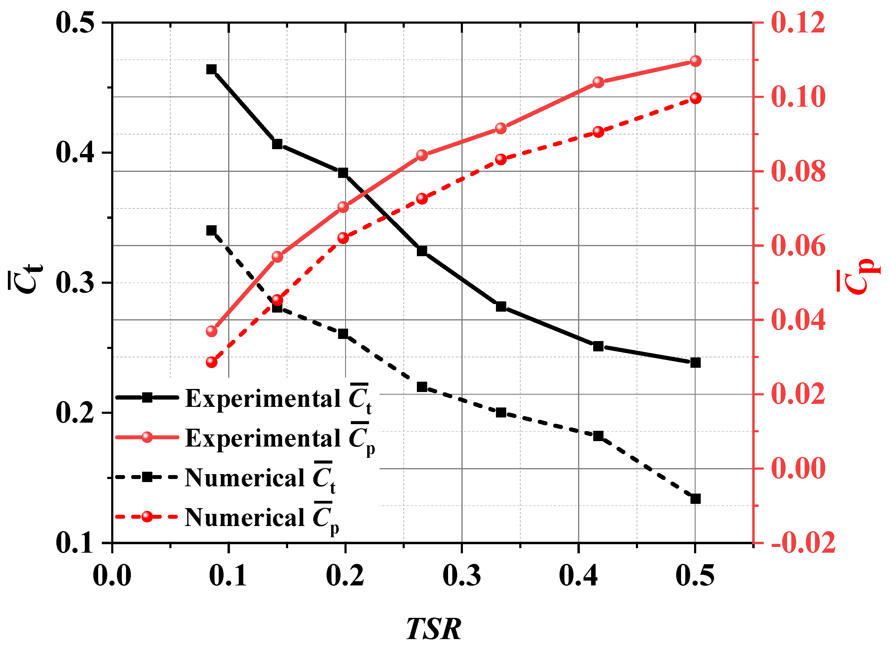
The startup process of a tulip-type hydraulic turbine rotor is investigated in this study. A CFD model is developed to analyze flow-driven rotor rotation, focusing on typical flow patterns and vortex behaviors around and downstream of the rotor. Comparisons with experimental data on rotor torque and power coefficient validate the accuracy of the model. This study emphasizes transient flow patterns and vortex evolution to clarify the startup mechanism of the rotor.

Rotor rotation involves three phases: initial, transition, and cyclic. The initial phase spans the rotor’s first half-turn, the transition phase occurs during the second half-turn, and subsequently, a cyclic flow pattern develops. The startup process includes the initial and transition phases.

The tulip-type rotor exhibits distinct flow characteristics compared to the conventional S-type rotor. Specifically, a pair of opposite-direction flows from behind the rotor due to two vortices, and fluid moves directly from upstream toward the convex side of the advancing blade before detaching near the blade tip. This behavior arises from the varying blade curvature diameter of the tulip-type rotor, unlike the constant curvature diameter of S-type blades. Surrounding vortices affect moment generation either positively or negatively, depending on their positions relative to the rotor. The interaction among these vortices significantly influences startup performance. Downstream vortices generate negative pressure regions on the convex surfaces of blades, contributing positively to rotational moment.

The expanded top design of the tulip-type rotor substantially improves startup performance through four distinct functions: smoothly guiding incoming flow, dissipating gap vortices, clearing vortices to prevent blockage, and enhancing fluid-blade interaction to increase energy transfer efficiency. The quantitative analyses of vortex strength, circulation, and drag coefficient further clarified the startup mechanism and provided essential data for future optimization and practical application of tulip-type turbines.

In conclusion, the main contribution of this study is the detailed identification of vortex evolution mechanisms and fluid-structure interactions governing the self-starting capability of the tulip-type rotor under low-speed flow conditions. These findings provide a theoretical basis for the design and optimization of tulip-type turbines for long-term, stable power generation in deep-sea observation systems. Future study will further investigate the rotor’s performance across a broader range of flow velocities and assess its energy conversion efficiency under actual oceanic conditions.

References

1. Khan, M.; Bhuyan, G.; Iqbal, M.; Quaicoe, J. Hydrokinetic energy conversion systems and assessment of horizontal and vertical axis turbines for river and tidal applications: A technology status review. Appl. Energy 2009, 86, 1823–1835. [Google Scholar] [CrossRef]
2. Eftekhari, H.; Al-Obaidi, A.S.M.; Eftekhari, S. Aerodynamic performance of vertical and horizontal axis wind turbines: A comparison review. Indones. J. Sci. Technol. 2022, 7, 65–88. [Google Scholar] [CrossRef]
3. Chen, J.; Yang, H.; Liu, C.; Lau, C.; Lo, M. A novel vertical axis water turbine for power generation from water pipelines. Energy 2013, 54, 184–193. [Google Scholar] [CrossRef]
4. Maldar, N.R.; Ng, C.Y.; Oguz, E. A review of the optimization studies for Savonius turbine considering hydrokinetic applications. Energy Convers. Manag. 2020, 226, 113495. [Google Scholar] [CrossRef]
5. Sarma, N.K.; Biswas, A.; Misra, R.D. Experimental and computational evaluation of Savonius hydrokinetic turbine for low velocity condition with comparison to Savonius wind turbine at the same input power. Energy Convers. Manag. 2014, 83, 88–98. [Google Scholar] [CrossRef]
6. Kang, C.; Zhao, H.; Li, B.; Gong, W.; Zhu, Y. Improvement of startup performance of the drag-type hydrokinetic rotor through two-stage configuration. Ocean Eng. 2021, 238, 109677. [Google Scholar] [CrossRef]
7. Nakajima, M.; Iio, S.; Ikeda, T. Performance of Double-step Savonius Rotor for Environmentally Friendly Hydraulic Turbine. J. Fluid Sci. Technol. 2008, 3, 410–419. [Google Scholar] [CrossRef]
8. Kumar, A.; Saini, R.P. Performance parameters of Savonius type hydrokinetic turbine–A Review. Renew. Sustain. Energy Rev. 2016, 64, 289–310. [Google Scholar] [CrossRef]
9. Wang, L.; Yeung, R.W. On the performance of a micro-scale Bach-type turbine as predicted by discrete-vortex simulations. Appl. Energy 2016, 183, 823–836. [Google Scholar] [CrossRef]
10. Talukdar, P.K.; Sardar, A.; Kulkarni, V.; Saha, U.K. Parametric analysis of model Savonius hydrokinetic turbines through experimental and computational investigations. Energy Convers. Manag. 2018, 158, 36–49. [Google Scholar] [CrossRef]
11. Tartuferi, M.; D’Alessandro, V.; Montelpare, S.; Ricci, R. Enhancement of Savonius wind rotor aerodynamic performance: A computational study of new blade shapes and curtain systems. Energy 2015, 79, 371–384. [Google Scholar] [CrossRef]
12. Mercado-Colmenero, J.M.; Rubio-Paramio, M.A.; Guerrero-Villar, F.; Martin-Doñate, C. A numerical and experimental study of a new Savonius wind rotor adaptation based on product design requirements. Energy Convers. Manag. 2018, 158, 210–234. [Google Scholar] [CrossRef]
13. Asim, T.; Singh, D.; Siddiqui, M.S.; McGlinchey, D. Effect of Stator Blades on the Startup Dynamics of a Vertical Axis Wind Turbine. Energies 2022, 15, 8135. [Google Scholar] [CrossRef]
14. Bhayo, B.A.; Al-Kayiem, H.H. Experimental characterization and comparison of performance parameters of S-rotors for standalone wind power system. Energy 2017, 138, 752–763. [Google Scholar] [CrossRef]
15. Kamoji, M.A.; Kedare, S.B.; Prabhu, S.V. Experimental investigations on single stage modified Savonius rotor. Appl. Energy 2009, 86, 1064–1073. [Google Scholar] [CrossRef]
16. Nasef, M.H.; El-Askary, W.A.; AbdEl-hamid, A.A.; Gad, H.E. Evaluation of Savonius rotor performance: Static and dynamic studies. J. Wind Eng. Ind. Aerodyn. 2013, 123, 1–11. [Google Scholar] [CrossRef]
17. Kamoji, M.A.; Kedare, S.B.; Prabhu, S.V. Performance tests on helical Savonius rotors. Renew. Energy 2009, 34, 521–529. [Google Scholar] [CrossRef]
18. Kacprzak, K.; Liskiewicz, G.; Sobczak, K. Numerical investigation of conventional and modified Savonius wind turbines. Renew. Energy 2013, 60, 578–585. [Google Scholar] [CrossRef]
19. Ghasemian, M.; Ashrafi, Z.N.; Sedaghat, A. A review on computational fluid dynamic simulation techniques for Darrieus vertical axis wind turbines. Energy Convers. Manag. 2017, 149, 87–100. [Google Scholar] [CrossRef]
20. Yang, W.; Hou, Y.; Jia, H.; Liu, B.; Xiao, R. Lift-type and drag-type hydro turbine with vertical axis for power generation from water pipelines. Energy 2019, 188, 116070. [Google Scholar] [CrossRef]
21. Mohamed, O.S.; Elbaz, A.M.R.; Bianchini, A. A better insight on physics involved in the self-starting of a straight-blade Darrieus wind turbine by means of two-dimensional Computational Fluid Dynamics. J. Wind Eng. Ind. Aerodyn. 2021, 218, 104793. [Google Scholar] [CrossRef]
22. Celik, Y.; Ma, L.; Ingham, D.; Pourkashanian, M. Aerodynamic investigation of the start-up process of H-type vertical axis wind turbines using CFD. J. Wind Eng. Ind. Aerodyn. 2020, 204, 104252. [Google Scholar] [CrossRef]
23. Asr, M.T.; Nezhad, E.Z.; Mustapha, F.; Wiriadidjaja, S. Study on start-up characteristics of H-Darrieus vertical axis wind turbines comprising NACA 4-digit series blade airfoils. Energy 2016, 112, 528–537. [Google Scholar] [CrossRef]
24. Kumar, R.; Raahemifar, K.; Fung, A.S. A critical review of vertical axis wind turbines for urban applications. Renew. Sustain. Energy Rev. 2018, 89, 281–291. [Google Scholar] [CrossRef]
25. Jacob, J.; Chatterjee, D. Design methodology of hybrid turbine towards better extraction of wind energy. Renew. Energy 2019, 131, 625–643. [Google Scholar] [CrossRef]
26. Bhuyan, S.; Biswas, A. Investigations on self-starting and performance characteristics of simple H and hybrid H-Savonius vertical axis wind rotors. Energy Convers. Manag. 2014, 87, 859–867. [Google Scholar] [CrossRef]
27. Li, Y.; Zhao, S.; Tagawa, K.; Feng, F. Starting performance effect of a truncated-cone-shaped wind gathering device on small-scale straight-bladed vertical axis wind turbine. Energy Convers. Manag. 2018, 167, 70–80. [Google Scholar] [CrossRef]
28. Gharib Yosry, A.; Fernández-Jiménez, A.; Álvarez-Álvarez, E.; Blanco Marigorta, E. Design and characterization of a vertical-axis micro tidal turbine for low velocity scenarios. Energy Convers. Manag. 2021, 237, 114144. [Google Scholar] [CrossRef]
29. Han, D.; Heo, Y.G.; Choi, N.J.; Nam, S.H.; Choi, K.H.; Kim, K.C. Design, fabrication, and performance test of a 100-W helical-blade vertical-axis wind turbine at low tip-speed ratio. Energies 2018, 11, 1517. [Google Scholar] [CrossRef]
30. Siram, O.; Saha, U.K.; Sahoo, N. Blade design considerations of small wind turbines: From classical to emerging bio-inspired profiles/shapes. J. Renew. Sustain. Energy 2022, 14, 042701. [Google Scholar] [CrossRef]
31. Kothe, L.B.; Möller, S.V.; Petry, A.P. Numerical and experimental study of a helical Savonius wind turbine and a comparison with a two-stage Savonius turbine. Renew. Energy 2020, 148, 627–638. [Google Scholar] [CrossRef]
32. Paul, S.; Reza, M.A.; Hossen, M.A.; Hossen, M.J.; Alam, M.J. Design and Manufacturing of a Tulip Type Wind Turbine to Harvest Electrical Energy. Ph. D. Thesis, Sonargoan University (SU), Dhaka, Bangladesh, 2023. [Google Scholar]
33. Kanthaiah, J.; Kumar, O.M.; Varma, M.R.; Kumar, M.M.; Sateesh, K. Tulip wind turbine. J. Eng. Sci. 2023, 14, 895–901. [Google Scholar]
34. Menter, F. In zonal two equation kw turbulence models for aerodynamic flows. In Proceedings of the 23rd Fluid Dynamics, Plasmadynamics, and Lasers Conference, Orlando, FL, USA, 6–9 July 1993; p. 2906. [Google Scholar]
35. Akwa, J.V.; Alves da Silva Júnior, G.; Petry, A.P. Discussion on the verification of the overlap ratio influence on performance coefficients of a Savonius wind rotor using computational fluid dynamics. Renew. Energy 2012, 38, 141–149. [Google Scholar] [CrossRef]
36. Subbulakshmi, A.; Verma, M.; Keerthana, M.; Sasmal, S.; Harikrishna, P.; Kapuria, S. Recent advances in experimental and numerical methods for dynamic analysis of floating offshore wind turbines—An integrated review. Renew. Sustain. Energy Rev. 2022, 164, 112525. [Google Scholar] [CrossRef]
37. Roy, S.; Saha, U.K. Review on the numerical investigations into the design and development of Savonius wind rotors. Renew. Sustain. Energy Rev. 2013, 24, 73–83. [Google Scholar] [CrossRef]
38. Janon, A. Torque coefficient analysis of a novel direct-drive parallel-stream counter-rotating Darrieus turbine system. Renew. Energy 2020, 147, 110–117. [Google Scholar] [CrossRef]
39. Dai, J.; Liu, D.; Wen, L.; Long, X. Research on power coefficient of wind turbines based on SCADA data. Renew. Energy 2016, 86, 206–215. [Google Scholar] [CrossRef]
Figure 1. Submarine power supply hydraulic turbines for geophysical instruments in deep-sea applications.
Jmse 13 01221 g001
Figure 2. (a) Tulip-type turbine rotor and (b) tulip flower.
Jmse 13 01221 g002
Figure 3. The tulip-type rotor: (a) tulip blade with four cross-sections (p1, p2, p3, and p4), (b) blade profile at p1, p2, p3, and p4, and (c) top view of the rotor.
Jmse 13 01221 g003
Figure 4. Schematic view of the computational domain for the tulip-type rotor.
Jmse 13 01221 g004
Figure 5. Cross-section distribution of grids on plane p3 of the rotor.
Jmse 13 01221 g005
Figure 6. Variation in C ¯ t with mesh number.
Jmse 13 01221 g006
Figure 7. (a) Experimental setup of the water tank test system and (b) schematic diagram of the test system configuration.
Jmse 13 01221 g007
Figure 8. (a) Experimental setup with a tulip-type rotor and (b) measurement positions of the flow meter.
Jmse 13 01221 g008
Figure 9. Model validation with experimental results for C ¯ t and C ¯ p .
Jmse 13 01221 g009
Figure 10. Variation in the rotor’s rotational velocity ω with the rotor’s rotation angle starting from θ = 90°.
Jmse 13 01221 g010
Figure 11. Typical flow pattern around tulip rotors under U = 4 m/s starting from θ = 90° in the (a) initial and (b) transition phase.
Jmse 13 01221 g011
Figure 12. Vortices from U = 4 m/s on the top p1, middle p3, and bottom p4 planes in the initial phase. The arrows overlaying the contours indicate local flow directions. Red solid arrows denote vortices that positively contribute to rotational moment generation, while blue dashed arrows represent vortices that negatively affect rotational moment generation.
Jmse 13 01221 g012
Figure 13. Vortices from U = 4 m/s on the top p1, middle p3, and bottom p4 planes in the transition phase. The arrows overlaying the contours indicate local flow directions. Red solid arrows denote vortices that positively contribute to rotational moment generation, while blue dashed arrows represent vortices that negatively affect rotational moment generation.
Jmse 13 01221 g013
Figure 14. Streamline distribution downstream of the rotor at the initial phase of θ = 135°, 180°, 225°, and 270°, as well as the pressure distributions and velocity vectors at the longitudinal x-y section A-A downstream of the rotor.
Jmse 13 01221 g014
Figure 15. Streamline distribution downstream of the rotor at the transition phase of θ = 315°, 360°, 405°, and 450°, as well as the pressure distributions and velocity vectors at the longitudinal x-y section A-A downstream of the rotor.
Jmse 13 01221 g015
Figure 16. Streamline distribution around the expanded top of the blade during the transition phase at (a) θ =315°, (b) 360°, (c) 405°, and (d) 450°.
Jmse 13 01221 g016
Figure 17. A general schematic of the flow pattern and vortex distribution around the entire tulip-type rotor.
Jmse 13 01221 g017