Abstract
Increasingly severe ocean acidification (OA) disrupts the balance of marine ecosystems. Seawater pH is a key indicator of OA but remains challenging to characterize due to sparse and limited in situ observations. In this study, we propose a spatiotemporal inversion method for surface pH based on interpretable machine learning. By applying carbonate system calculations, we construct an expanded pH observational dataset and obtain spatiotemporal distributions of pH and its influencing factors across the Pacific Ocean from 2003 to 2021. The interpretability analysis reveals that physical, biological, and optical factors contribute 53.9%, 23.9%, and 22.2%, respectively, to pH variability. Sea-surface temperature is the dominant driver, contributing 15.9% of all factors by regulating CO2 solubility and biological activity. Particulate inorganic carbon (PIC) and particulate organic carbon (POC) show relative contributions of 12.6% and 9.4%, respectively, quantitatively reflecting the important roles of biogenic calcification and the biological carbon pump. Furthermore, the analysis focusing on the Niño 3.4 region reveals a potential pathway through which the ENSO disturbances may affect pH by influencing PIC and POC. Therefore, this study provides a data-driven approach to gain deeper insights into the spatiotemporal patterns of pH and its influencing factors.
1. Introduction
The ocean, as the Earth’s largest carbon reservoir, plays a vital role in regulating the stability of the global climate system by absorbing anthropogenic carbon dioxide (CO2) emissions [1]. Since the Industrial Revolution, the ocean has sequestered approximately 30% of human-induced CO2 emissions, mitigating atmospheric warming while inducing significant alterations to seawater chemistry [2]. The surface ocean pH has been declining at a rate of 0.0022 units per year, resulting in an overall decrease of about 0.1 units relative to pre-industrial levels [2]. This disruption of the carbonate system, known as ocean acidification (OA), has been identified, along with global warming and biodiversity loss, as one of the three major environmental crises of the 21st century. If current CO2 emission trends persist, surface ocean pH is projected to decrease by an additional 0.3–0.4 units by 2100, with a 150% increase in hydrogen ion concentration, severely threatening calcifying organisms such as corals and shellfish and cascading through marine food webs to impact fisheries and coastal ecosystems [3].
Among global oceans, the Pacific has drawn particular attention due to its unique geographic and climatic features. As the largest ocean basin, it accounts for nearly 60% of the global oceanic CO2 uptake [4] and exhibits pronounced spatiotemporal heterogeneity in acidification rates and ecological responses. Studies have shown that equatorial Pacific upwelling brings CO2-rich deep waters to the surface, resulting in pH decline rates that are 30% higher than the global average [5]. In the North Pacific subpolar region, seasonal fluctuations cause summer pH variations of up to 0.15 units [6]. Additionally, the Southern Ocean carbon sink weakened during the 1990s, accelerating atmospheric CO2 accumulation and OA, although it has shown signs of recovery over the past decade, highlighting its dynamic nature [7]. The strong coupling between the Pacific Ocean and atmospheric circulation modes, such as ENSO and PDO, further complicates the dynamics of acidification [8]. Nevertheless, limited by fragmented observational coverage, significant gaps remain in our understanding of the fine-scale spatiotemporal patterns, dominant driving mechanisms, and cascading ecological impacts of Pacific OA.
In recent years, research on OA has advanced rapidly, with most studies focusing on the impacts of acidification on calcium carbonate saturation states, marine organisms, and the ecosystems they inhabit. Traditional approaches often involve establishing models or empirical formulas based on observational data to simulate physical, chemical, and biological processes in the ocean, thereby determining seawater pH. From the perspective of numerical simulation, numerous complex biogeochemical and coupled models have been applied at both global and regional scales to investigate ecological and environmental issues concerning OA.
Caldeira et al. [9] quantified the potential changes in ocean pH resulting from continuous CO2 emissions by using a four-box ocean–atmosphere model. They estimated the historical influence of atmospheric CO2 on ocean pH and found that oceanic uptake of CO2 from fossil fuels could cause future pH changes greater than any inferred value from the geological record of the past 300 million years. Gruber et al. [10] integrated dynamic ocean circulation models with observational data to investigate anomalous acidification in the California Current, revealing significant seasonal variability in nearshore pH (up to 0.2 units) within 50 km of the coast. However, these calculations often neglected important factors, such as physical diffusion and atmospheric CO2 concentration, which limited the accuracy of their results. In another study, Feely et al. [11] used a biogeochemical ocean general circulation model (BOGCM) to describe current pH conditions and global OA induced by CO2 uptake. While physical models provide a comprehensive understanding of the Earth’s systems, their capacity to characterize nonlinear marine biogeochemical processes and ecosystem dynamics remains limited.
With the continuous launch of Earth observation satellites, the volume of remotely sensed data has grown substantially, enabling the development of data-driven models for surface-seawater pH estimation. In recent years, machine learning methods have proliferated, leading to ongoing improvements in algorithm performance of remote sensing retrieval and relationship mining. These approaches provide a promising alternative for pH estimation by reducing reliance on prior knowledge of oceanography. However, the global distribution of in situ pH measurements remains sparse and uneven, presenting a significant challenge for scaling up pH studies. Previous research typically employed regression models based on limited observational data. For example, Wootton et al. [12] developed a regression model for seawater pH using least-squares fitting, incorporating a range of physical, chemical, and biological variables such as sea level, photosynthesis, temperature, upwelling, phytoplankton abundance, the PDO index, alkalinity, and salinity.
To address the lack of detailed temporal variability (e.g., annual, seasonal, and monthly scales) in observational data, Li et al. [13] utilized dissolved oxygen, temperature, and salinity data from the CLIVAR and PACIFICA datasets to establish a multiple linear regression model. Their model achieved a high accuracy and reconstructed the vertical distributions (40–400 m) of total alkalinity (TA), dissolved inorganic carbon (DIC), and pH in the subarctic North Pacific from 2000 to 2010. Machine learning techniques are particularly effective in modeling complex systems with high-dimensional data or large scale, often yielding robust fitting performance. Krishna et al. [14] considered chlorophyll-a concentration (Chl-a), sea-surface temperature (SST), and sea-surface salinity (SSS) as key biogeochemistry drivers to establish multivariate nonlinear regression relationships with in situ measurements on a global scale. By using satellite data and a segmented modeling approach, the resulting prediction error for surface-seawater partial pressure of CO2 (pCO2) ranged between 6.12 and 8.77 µatm. Iida et al. [15] developed empirical relationships between sea-surface temperature, salinity, Chl-a concentration, and mixed-layer depth (MLD) with DIC and TA, leading to the generation of a global 1° × 1° monthly DIC/TA dataset for the period 1993–2021. An analysis of the dataset revealed a phase-dependent evolution in the oceanic carbon sink over the past three decades: a decline in carbon uptake efficiency during the 1990s followed by a recovery and enhancement in the 21st century. The global downward trend in seawater pH was found to be significantly correlated with the increase in atmospheric CO2 concentration. To mitigate the issue of severely limited in situ pH observations, Jiang et al. [16] proposed a novel approach that directly inverts pH values from remote sensing data. By first estimating TA using sea-surface salinity and related parameters and then calculating carbonate parameters using large-scale underway pCO2 measurements, they generated a near-observational volume of pH data, thereby addressing the data shortage problem for algorithm development. Zhong et al. [17] employed a self-organizing map (SOM) neural network to divide the global ocean into 14 biogeochemical provinces and, in combination with a stepwise feedforward neural network (FFNN), constructed the first global monthly seawater pH dataset covering 0–2000 m depth at a spatial resolution of 1° × 1° for the period 1992–2020. The dataset achieved a root mean square error (RMSE) of 0.028 when compared with in situ observations and effectively captured surface acidification trends, as validated against long-term time-series station data.
While traditional models can simulate the distribution and temporal trends of pH to some extent, they require substantial prior knowledge about the study region, increasing the complexity of model initialization. Furthermore, they exhibit limited capability in capturing the large-scale spatiotemporal heterogeneity of surface-seawater pH. The short period and sparse, uneven spatial coverage of observational data significantly constrain the effective reconstruction of continuous pH fields, posing major challenges for analyzing the spatiotemporal characteristics of OA. However, existing data-driven approaches often operate as black boxes, lacking the ability to quantify the relative influence of input variables, which impedes the analysis of spatiotemporal variability in the drivers of OA.
To address these issues, we first applied a machine learning model to estimate TA based on strongly correlated physical parameters. Subsequently, we employed carbonate system calculations to infer pH, thereby expanding the sparse observational dataset of pH. Finally, using an interpretable machine learning framework and multisource data, we achieved the retrieval of pH across the Pacific Ocean. Furthermore, we quantitatively assessed the contributions of physical, biological, and optical factors to the OA based on the interpretable machine learning.
2. Data and Methods
2.1. Study Area and Data
The combined effects of oceanic physical dynamics, chemical reactions, and biological processes shape surface-seawater pH. The complex and dynamic nature of OA necessitates extensive data support for long-term, large-scale pH reconstruction. Key factors influencing surface pH include SST [18], SSS [19], TA, CO2 fugacity (fCO2) [20], dissolved oxygen [21], and Chl-a [22]. Additionally, physical factors such as upwelling [23], MLD, and zonal and meridional surface wind speeds, as well as optical properties derived from ocean-color remote sensing, also exert indirect influences. Accordingly, this study integrates these factors to facilitate the high-spatiotemporal-resolution inversion of surface pH across the Pacific Ocean.
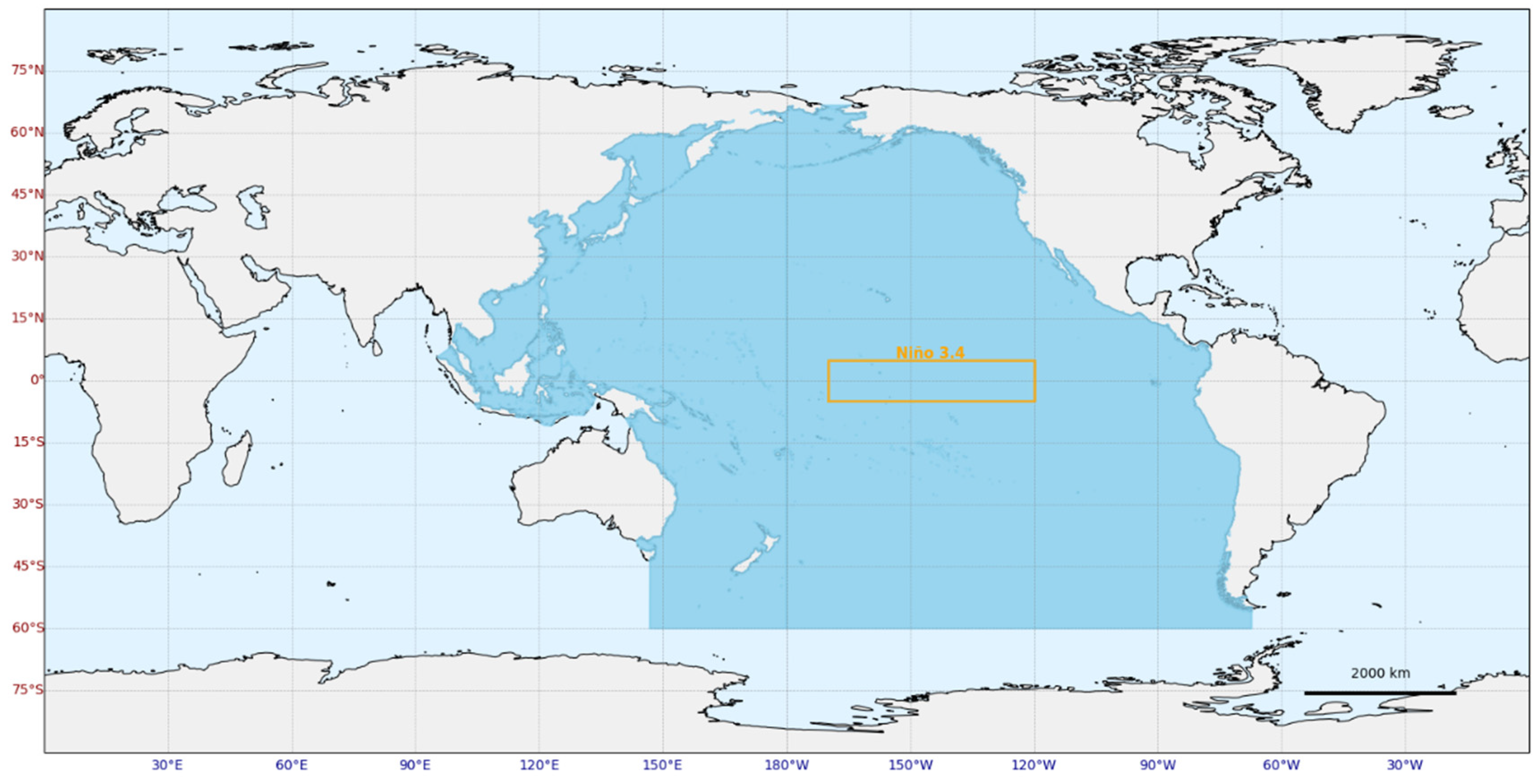
Due to its status as the largest ocean basin, responsible for approximately 60% of global oceanic CO2 uptake, and its significant spatiotemporal variability in acidification dynamics and ecological responses, the Pacific Ocean was chosen as the study region. Special attention was directed toward the Niño 3.4 region, which plays a crucial role in ENSO-related variability, as shown in Figure 1.
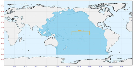
Figure 1.
The study area. The orange rectangle is the Niño 3.4 region.
All the research data was listed in Table 1. For in situ data, we utilized datasets from the Global Ocean Data Analysis Project (GLODAP) [24] and the Surface Ocean CO2 Atlas (SOCAT). To ensure consistency between field measurements and satellite observations, we selected measurements from 2003 to 2023 that were quality-controlled with WOCE flags 0 and 2 [25] and limited to sampling depths of less than 10 m. In total, 10,358 samples of SST, SSS, and TA were collected and used for the construction of the total alkalinity model and validation of the pH inversion results.

Table 1.
Research data, including in situ data, remote sensing data, and reanalysis data.
This study utilized remote sensing, reanalysis, and in situ datasets covering the period from 2003 to 2021. Remote sensing data were obtained from NASA’s MODIS-Aqua Ocean Color dataset, which includes Chl-a, diffuse attenuation coefficient at 490 nm (KD), particulate organic carbon (POC), and particulate inorganic carbon (PIC), all at a spatial resolution of 4 km. Meteorological data were sourced from the ERA5 reanalysis product of the European Centre for Medium-Range Weather Forecasts (ECMWF), encompassing 10 m zonal and meridional wind components (u10, v10), sea-level pressure (Pressure), and total precipitation (Precipitation), with a spatial resolution of 0.25°.
Ocean physical variables were obtained from the Global Ocean Physics Reanalysis (GOPR) provided by the Copernicus Marine Environment Monitoring Service (CMEMS). The selected variables included sea-surface height (SSH), MLD, and sea-surface salinity (SSS), with a spatial resolution of 0.83°. These datasets collectively provided comprehensive inputs for the high-resolution spatiotemporal inversion of surface-seawater pH.
2.2. Calculation of the Seawater Carbonate System
With the continuous rise in atmospheric CO2 concentrations, the ocean absorbs excess CO2, disrupting the carbonate equilibrium and resulting in the formation of carbonic acid and the release of hydrogen ions. Consequently, seawater pH gradually decreases, contributing to OA. The carbonate system can be divided into four equilibrium processes: CO2 dissolution equilibrium, CO2 hydration equilibrium, carbonic acid dissociation equilibrium, and bicarbonate dissociation equilibrium. The corresponding chemical reactions and dissociation constants are as follows:
In addition to , three additional parameters are required to characterize the seawater carbonate system: , , and . These parameters are defined as follows:
In Equation (7), since bicarbonate and carbonate together account for over 96% of TA, TA can be approximated as carbonate alkalinity .
If any two of the four key parameters (, and ) are known, the remaining two can be calculated using the carbonate system equations. In this study, PyCO2SYS (https://pyco2sys.readthedocs.io/en/latest/, accessed on 21 April 2023) was used to compute (on the total scale) at corresponding seawater temperature conditions. The sulfuric acid dissociation constant was used as the standard reference [26], while the carbonate dissociation constants were derived from the empirical seawater constants proposed by Lueker et al. [20].
To ensure consistency, seawater temperature was set within the range of 2–35 °C and salinity between 19 and 43 psu. Additionally, before calculating pH, SOCAT data were filtered according to these predefined temperature and salinity criteria.
2.3. Model and Methodology Description
This study employed several machine learning models for comparison, including Logistic Regression (LR), Support Vector Regression (SVR), Random Forest (RF), Gradient Boosting Decision Tree (GBDT), and Extremely Randomized Trees (ExtraTrees), eXtreme Gradient Boosting (XGBoost).
The tree model predicts the value of the target variable by recursively partitioning the feature space, which has advantages such as handling nonlinear relationships. In XGBoost, each successive base model minimizes the residuals between predicted and true values by computing the negative gradient of the previous tree’s loss function, which serves as the basis for the new tree’s construction. This process effectively reduces system errors.
XGBoost also incorporates key features such as sample weighting, sparse feature learning, and strategies to prevent overfitting. Additionally, it improves computational efficiency through parallel optimization, buffering techniques, and out-of-core computation, making it especially suitable for large-scale and imbalanced datasets.
The XGBoost model predicts outcomes using an additive framework composed of K tree models:
where represents the predicted value of the model, denotes the number of tree models, corresponds to the -th tree model, and represents the feature space of the base model.
This study incorporates the SHapley Additive exPlanations (SHAP) method to analyze the contribution of individual input factors to the model. SHAP is a machine learning interpretability module based on Shapley value theory from game theory that effectively quantifies the contribution of each feature to the model’s predictions, thereby enhancing model transparency interpretability.
The SHAP value for feature is calculated using the following formula:
where represents the set of all features, and denotes the model’s predicted value for the feature subset .
2.4. An Interpretable Machine Learning Approach for Spatiotemporal Inversion of Sea Surface pH
- (1)
- Figure 2 illustrates the methodological framework of this study. The modeling of ocean carbonate system parameters was carried out through the following steps:
- (2)
- The preprocessing of the GLODAP and SOCAT datasets included standardization, spatial filtering, temperature–salinity screening, and outlier removal. In situ observations were integrated with satellite and reanalysis datasets to construct the TA inversion model. All remote sensing and reanalysis products were resampled to a uniform spatial resolution of 8 × 8 km using bilinear interpolation. For each in situ sampling location, the corresponding environmental variable values were extracted from the resampled datasets based on geographic coordinates and sampling date.
- (3)
- The construction of TA inversion models utilizing various machine learning methods based on two sets of input features: (SST, SSS) and (SST, SSS, Chl-a), with in situ TA measurements from GLODAP dataset.
- (4)
- The optimal TA inversion model is selected to expand the TA observational dataset by integrating it with the preprocessed SOCAT dataset. Surface pH values are then estimated using carbonate system calculations based on SOCAT fCO2 data and the optimal TA model.
- (5)
- The development of an expanded surface pH dataset for the Pacific Ocean. Using this dataset, an interpretable machine learning model was trained to produce pH inversion results, and SHAP analysis was applied to quantify and attribute the contributions of influencing factors to pH variability.
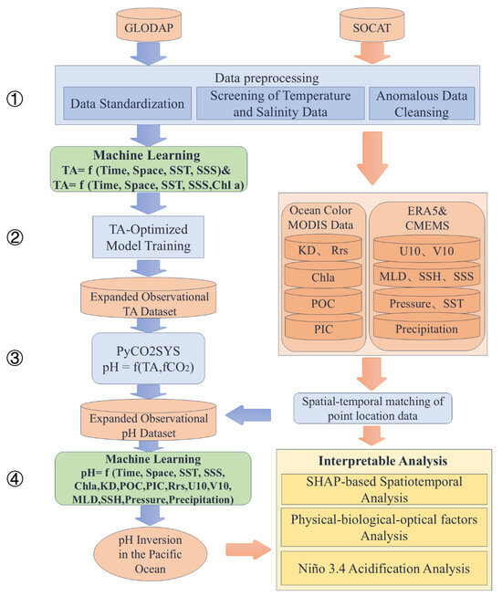
Figure 2.
An interpretable machine learning approach for spatiotemporal inversion of sea-surface pH.
Figure 2.
An interpretable machine learning approach for spatiotemporal inversion of sea-surface pH.

2.5. Model Evaluation Metrics and Model Configuration
In this study, the XGBoost algorithm was applied to reconstruct TA and surface-seawater pH in the Pacific Ocean. To evaluate the model’s performance, a ten-fold cross-validation approach was adopted, with the dataset split into a 9:1 training-to-test ratio.
Ten-fold cross-validation is a widely used statistical method for assessing a machine learning model’s generalization ability. The core concept involves randomly partitioning the dataset into ten mutually exclusive subsets of approximately equal size. In each iteration, one subset is designated as the test set, while the remaining nine subsets are used for training. This process is repeated ten times, and the average result is reported as the final evaluation of the model’s performance.
To assess the accuracy and reliability of the carbonate system inversion results, four evaluation metrics were applied: Coefficient of Determination (R2), RMSE, Mean Absolute Error (MAE).
The calculation formulas for each metric are as follows:
where represents the number of observations, denotes the observed (true) value, and is the predicted value. and are the mean values of and respectively, calculated over the range .
To ensure the robustness and reproducibility of the machine learning models, we conducted extensive hyperparameter tuning using a grid search strategy. The specific hyperparameter settings tested for each model are summarized in Table 2.
Table 2.
Hyperparameter settings used for model selection.
3. Results
3.1. Reconstruction Results of Observed Total Alkalinity Data
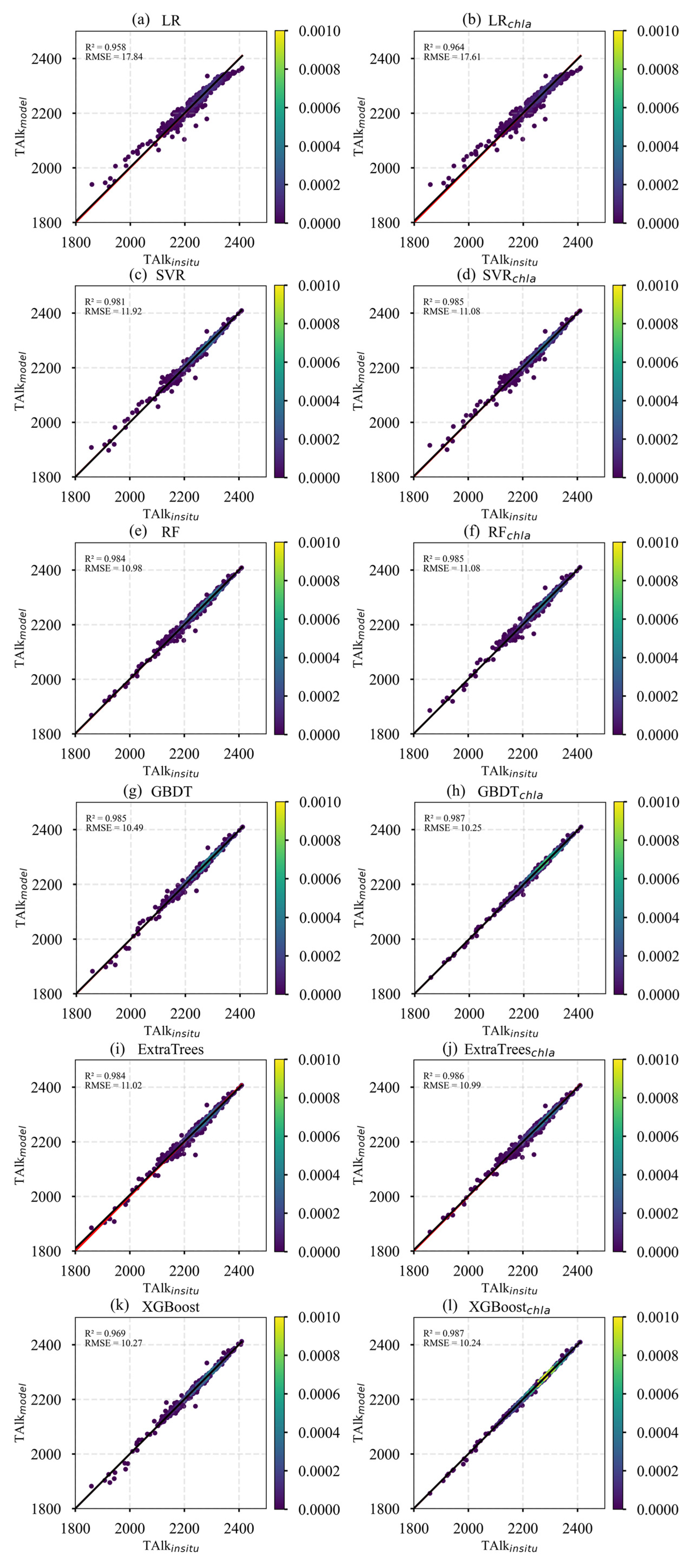
In this study, six machine learning models—LR, SVR, RF, GBDT, ExtraTrees, and XGBoost—were systematically evaluated to model surface TA in the Pacific Ocean. Two combinations of input features were tested: (SST, SSS) and (SST, SSS, Chl-a), with model training based on in situ TA measurements from the GLODAP dataset.
Table 3 summarizes the performance of the six models using different feature sets on the TA test dataset. At the model level, GBDT, ExtraTrees, and XGBoost achieved the best results. For the first feature set (SST and SSS), LR recorded the lowest R2, RMSE, and MAE values among all models. In contrast, GBDT, ExtraTrees, and XGBoost all achieved R2 values exceeding 0.985, RMSE values below 11, and MAE values below 6.5, indicating minor differences in performance and confirming their suitability for reconstructing surface TA in the Pacific Ocean. For the second feature set (SST, SSS, and Chl-a), the XGBoost-based model demonstrated the best performance, achieving the highest R2 of 0.987 and the lowest RMSE and MAE values.
Table 3.
Performance evaluation of TA modeling on the test set.
To further compare the performance of different models, scatter plots of predicted versus observed values were generated, as shown in Figure 3. The LR and SVR models exhibited significant dispersion in the low-value range, indicating limited predictive capability for lower TA values. Additionally, the slopes of their fitted lines deviated positively from the 1:1 line, suggesting a tendency to overestimate low values. In contrast, the scatter points for ExtraTrees, GBDT, and XGBoost were tightly clustered and closely aligned along the 1:1 line, with XGBoost demonstrating the best overall fit performance.
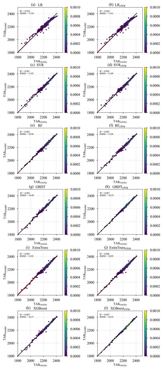
Figure 3.
Scatter plots of predicted versus observed TA for different models.
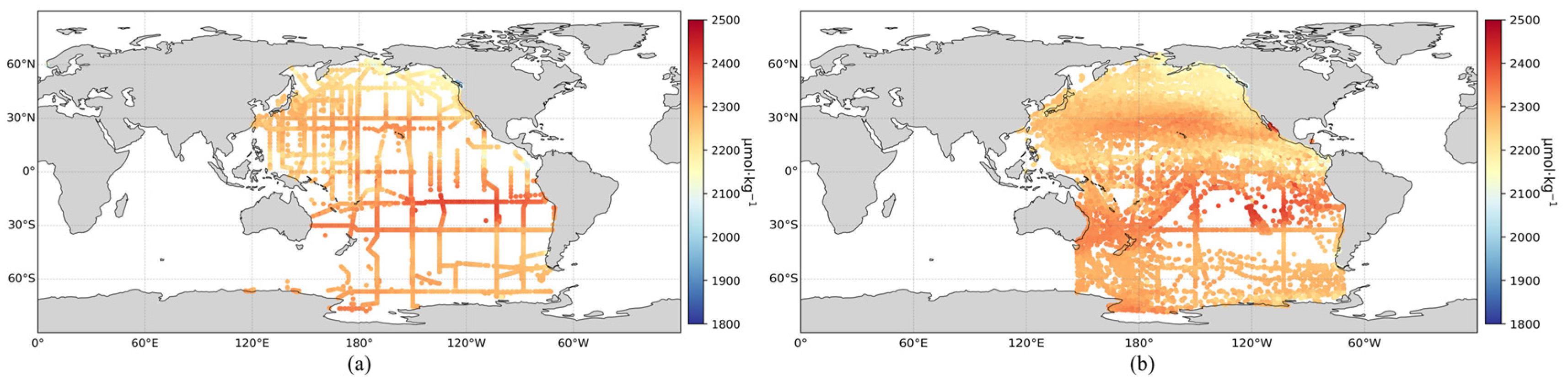
Based on the optimal XGBoost inversion model and the SOCAT dataset, an expanded surface TA dataset for the Pacific Ocean was created. To assess the consistency with actual observations, the spatial distribution of surface TA from the GLODAP dataset was also mapped. As shown in Figure 4, the expanded TA dataset closely aligns with the spatial distribution of the in situ GLODAP measurements. Moreover, the expanded dataset significantly enhances the temporal and spatial coverage compared to the original GLODAP dataset.
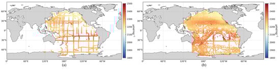
Figure 4.
(a) Observed surface TA distribution in the Pacific Ocean; (b) Expanded surface TA distribution in the Pacific Ocean.
3.2. Reconstruction Results of Observed pH Data
Based on the model evaluation results, the XGBoost model utilizing SST, SSS, and Chl-a as input variables outperformed the model that used only SST and SSS. Consequently, this optimal model was chosen to construct an expanded surface TA dataset for the Pacific Ocean using the SOCAT dataset. By applying carbonate system calculations, the expanded TA dataset and SOCAT fCO2 measurements were employed to generate an expanded surface pH dataset, resulting in 1,082,689 pH data points.
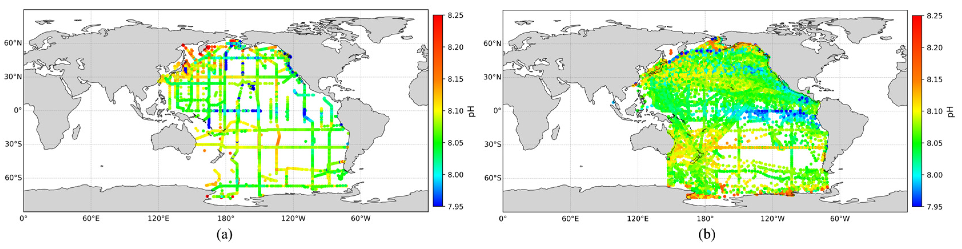
To assess the accuracy of the expanded pH dataset and compare it with actual observations, the spatial distribution of pH values from the GLODAP dataset was plotted alongside the expanded dataset, as shown in Figure 5. The results demonstrate that the expanded pH dataset closely matches the spatial patterns of GLODAP observations. Furthermore, it significantly enhances temporal and spatial coverage, particularly in areas with previously sparse observations, such as the South Pacific. This expanded pH dataset provides a solid foundation for the subsequent large-scale inversion of surface ocean pH across the Pacific.

Figure 5.
(a) Observed surface pH distribution in the Pacific Ocean; (b) Expanded surface pH distribution in the Pacific Ocean.
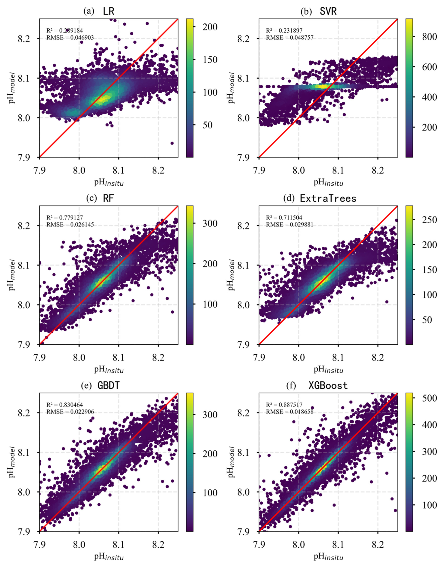
In this study, six models—LR, SVR, RF, GBDT, ExtraTrees, and XGBoost—were employed to invert surface ocean pH, using 20 features that encompass remote sensing, meteorological, and physical variables. Table 4 summarizes the test set performance of each model, presenting R2, RMSE, and MAE metrics for comparison. The results indicate that LR and SVR demonstrated the poorest performance, suggesting their limited ability to capture the complex variability of Pacific Ocean pH. In contrast, XGBoost consistently achieved the highest R2 and the lowest RMSE and MAE, demonstrating superior performance and greater suitability for modeling such complex oceanographic processes.
Table 4.
Performance evaluation of pH modeling on test set.
To further assess the performance of each regression model in predicting surface pH in the Pacific Ocean, scatter plots of predicted versus observed values were generated to visually evaluate model accuracy. As shown in Figure 6, significant differences in prediction accuracy and data distribution are evident across the models. The LR and SVR models exhibited poor predictive performance, characterized by high dispersion and an inability to effectively capture pH variability. The RF, ExtraTrees, and GBDT models performed considerably better, with most data points clustering near the 1:1 line, although some deviations remained. XGBoost achieved the best overall performance, demonstrating the highest accuracy. We compared the studies by Zhong [17] and Jiang [16], whose surface pH inversion models achieved RMSE values of 0.03 and 0.009, respectively. In contrast, the RMSE of our model is 0.00186, demonstrating superior performance to both. Its scatter plot displayed the closest alignment with the 1:1 line, reflecting its superior predictive capability. Overall, XGBoost showed the highest R2 and the lowest RMSE and MAE among all models, indicating its strong ability to accurately capture the spatiotemporal variability of surface pH in the Pacific Ocean.
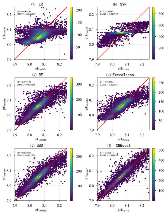
Figure 6.
Scatter plots of predicted versus observed pH values for different models. (The red line is 1:1 line).
3.3. Spatiotemporal Inversion Results of Sea-Surface pH
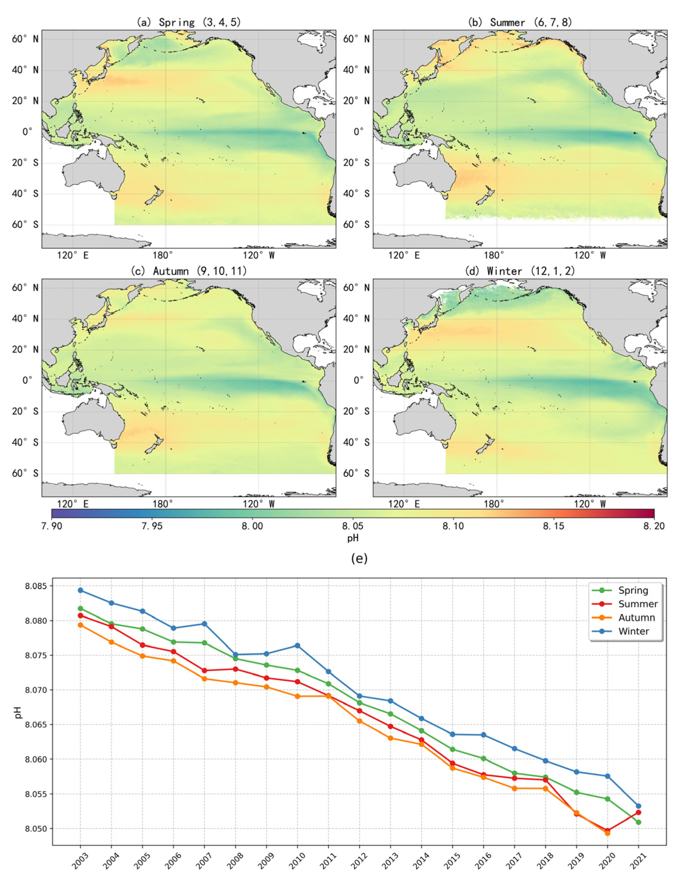
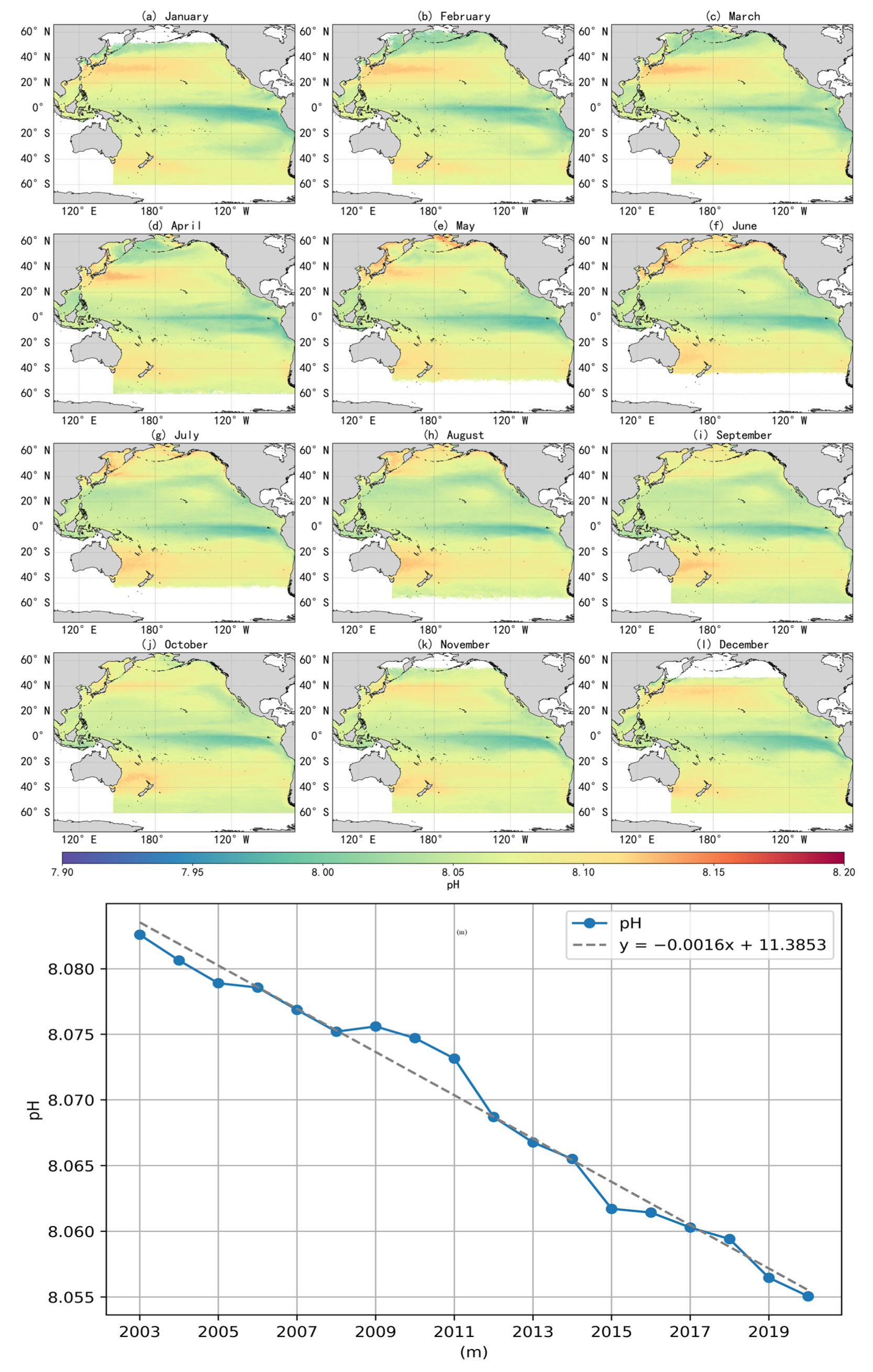
Based on the optimal pH inversion model, this study reconstructed the surface pH distribution across the Pacific Ocean at an 8 km × 8 km spatial resolution for the period 2003–2021, producing seasonal maps of surface-seawater pH (Figure 7). The spatial distribution of pH exhibited a clear latitudinal gradient and pronounced spatial heterogeneity. The equatorial Pacific and the eastern Pacific upwelling regions displayed the lowest pH values, with acidified conditions particularly evident, likely driven by the upwelling of CO2-rich deep waters that disrupt carbonate system equilibrium [11]. In contrast, higher pH values were observed in regions at mid to high latitudes such the Kuroshio Extension (KE) region, possibly associated with the downward transport of carbon [27].
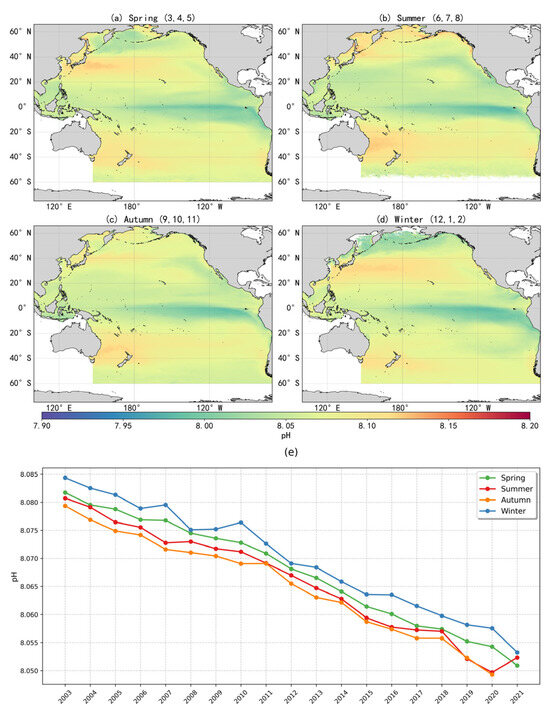
Figure 7.
(a–d) Seasonal distribution of mean surface-seawater pH in the Pacific Ocean (2003–2021); (e) Interannual variability of seasonal mean surface-seawater pH in the Pacific Ocean (2003–2021).
Additionally, the North Pacific subtropical gyre exhibited slightly lower pH values compared to the East Australian Current region and the South Pacific mid–high latitudes, likely reflecting limited biological activity [6]. Seasonal phytoplankton blooms in high-latitude areas may temporarily elevate pH through short-term CO2 drawdown, while variations in upwelling intensity and vertical mixing further contribute to the complex distribution patterns of pH [10]. This spatial variability may reflect the influence of large-scale ocean circulation, variations in biological carbon pump efficiency, freshwater inputs, and air–sea CO2 exchange. Although pH values in the South Pacific are generally higher than those at the equator, they remain lower when compared to corresponding latitudes in the Northern Hemisphere. This hemispheric asymmetry is likely related to natural upwelling processes driven by the Antarctic Circumpolar Current and differing levels of anthropogenic impact between hemispheres.
The trend in annual mean surface-seawater pH across the Pacific Ocean from 2003 to 2021, along with the fitted curve, is illustrated in Figure 8m. The annual means were calculated from monthly averaged data. During this period, surface pH showed a consistent declining trend, with an estimated rate of –0.0016 units per year. If this trend continues, the global surface ocean pH is projected to decline by approximately 0.128 units by the end of the century, corresponding to a 34.3% increase in hydrogen ion concentration. Such changes would diminish the ocean’s ability to buffer and absorb anthropogenic CO2. The pH decline rate identified in this study is generally consistent with the findings from long-term time-series observations reported by Bates et al. [28] and with the Copernicus Marine Environment Monitoring Service report [29].
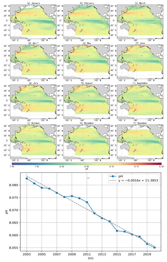
Figure 8.
The monthly spatial distribution (a–l) and interannual variability (m) of sea-surface pH in the Pacific Ocean from 2003 to 2021.
4. Discussion
4.1. Analysis of Factors Influencing Surface pH in the Pacific Ocean
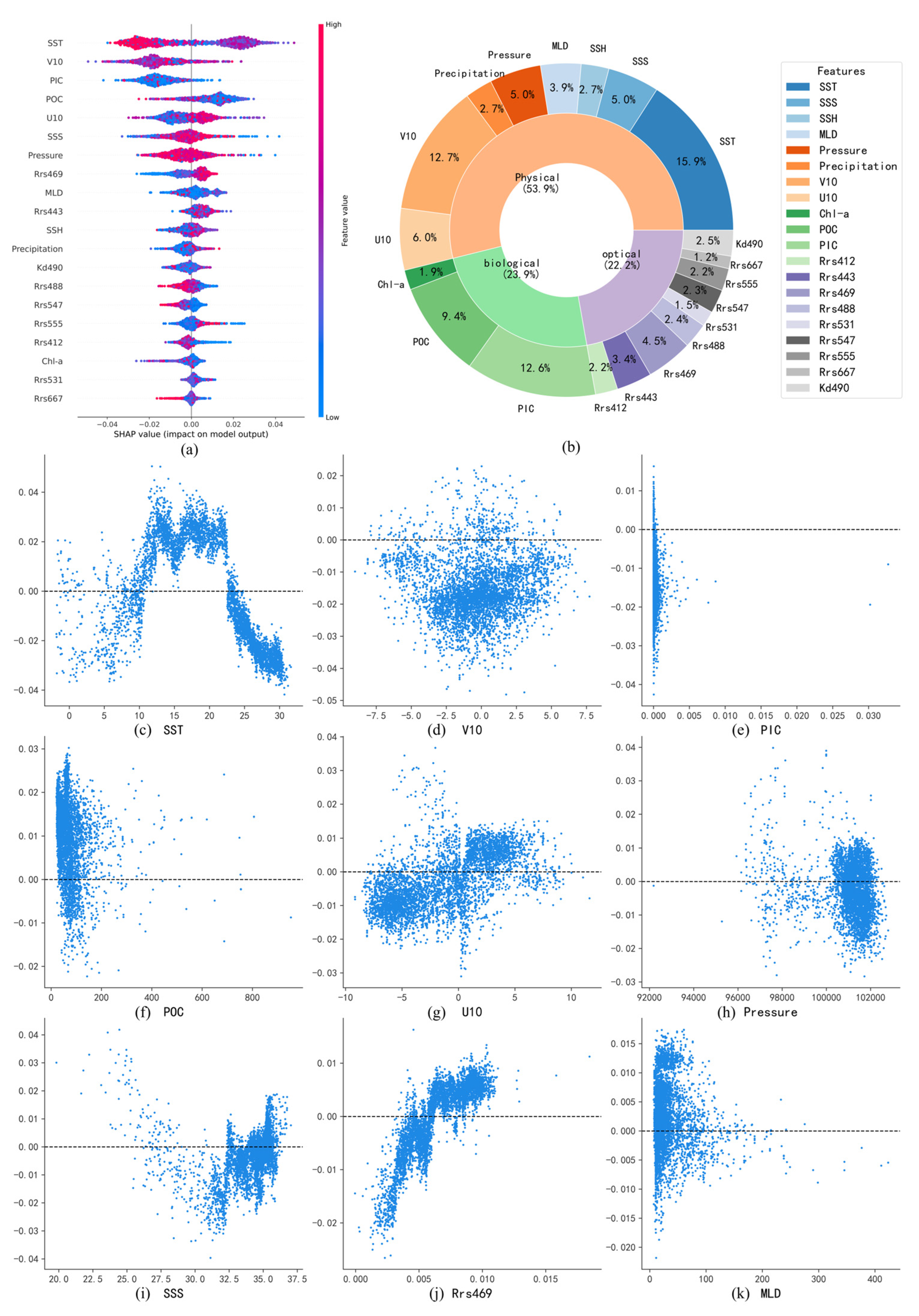
In this study, the SHAP method was utilized to interpret the potential drivers influencing surface pH. All input variables were organized into three categories: physical factors (SST, SSS, SSH, MLD, pressure, precipitation, and U/V10), biological factors (Chl-a, POC, and PIC), and optical factors (including Rrs412, Rrs443, Rrs469, and other remote sensing reflectance parameters). By creating feature importance plots and dependence plots, SHAP provided an interpretable, model-based assessment of how each input variable affected the model’s pH predictions. While this approach emphasizes the variables that the model relies on most, it does not imply statistical significance in a hypothesis-testing context. Therefore, the analysis offers a valuable exploratory perspective on potential influencing factors, rather than the attribution of definitive causal claims.
Figure 9a illustrates the relative influence of various environmental variables on the predicted surface-seawater pH in the Pacific Ocean using the SHAP method. The impact of each variable is represented by the distribution of SHAP values, with larger deviations from zero indicating stronger contributions to the pH prediction. The color gradient, ranging from blue (low values) to red (high values), signifies the magnitude of the variables themselves. Variables such as SST, PIC, and POC exhibit broad distributions of SHAP values, indicating significant influences on the model’s outcomes. In contrast, variables like Rrs667, Rrs531, and Chl-a have SHAP values clustered near zero, suggesting limited contributions.
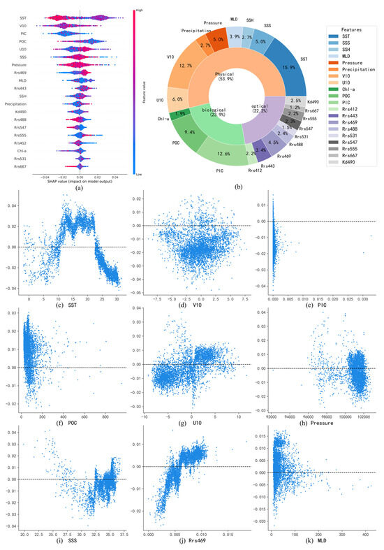
Figure 9.
(a,b) Summary of pH-influencing factors and their relative contributions in the Pacific Ocean; (c–k) Dependence plots of major pH-influencing factors in the Pacific Ocean.
Figure 9b further quantifies the relative contributions of these influencing factors. Physical factors collectively dominate, accounting for 53.9% of the total contribution, underscoring their crucial role in regulating surface-seawater pH. Biological factors contribute 23.9%, primarily driven by PIC and POC, while Chl-a plays a relatively minor role, likely due to the more significant impact of particulate carbon on seawater acidity. Optical factors contribute 22.2%, which is comparable to the contribution of biological factors.
SHAP dependence plots of major influencing factors reveal relationships consistent with previous numerical modeling studies. For SST, distinct latitudinal patterns emerge: at low latitudes (>20 °C), SST exhibits a negative correlation with pH, as increased temperatures promote bicarbonate (HCO3−) dissociation, generating hydrogen ions (H+) and reducing pH. Meanwhile, the stratification of water caused by high temperatures may also inhibit the downward transport of carbon. At moderate latitudes (10–20 °C), SST shows a positive correlation with pH, reflecting the enhanced CO2 uptake through phytoplankton photosynthesis, which offsets direct temperature-induced acidification. At high latitudes, SST again negatively correlates with pH, likely due to enhanced CO2 solubility at lower temperatures, which drives increased CO2 uptake and subsequent acidification [30].
For PIC (Figure 9e), SHAP values primarily show negative contributions to pH. Elevated PIC concentrations generally indicate active calcification by marine organisms, which release hydrogen ions and increase acidification. However, positive correlations between PIC and pH are observed in certain regions, possibly due to suppressed calcification under severe acidification conditions in eastern Pacific upwelling zones, resulting in simultaneously low PIC and low pH [31].
In more cases, POC (Figure 9f) exhibits positive correlations with pH. Higher POC typically indicates active phytoplankton carbon fixation, which mitigates acidification by converting dissolved CO2 into organic carbon [32]. However, negative correlations between POC and pH are observed in localized upwelling areas of the eastern Pacific, where high POC concentrations correspond with low pH due to continuous replenishment by CO2-rich deep waters.
SSS demonstrates a nonlinear relationship with pH (Figure 9i), indicating positive contributions at both lower and higher extremes of salinity. However, the underlying mechanisms of this relationship require further investigation and exploration.
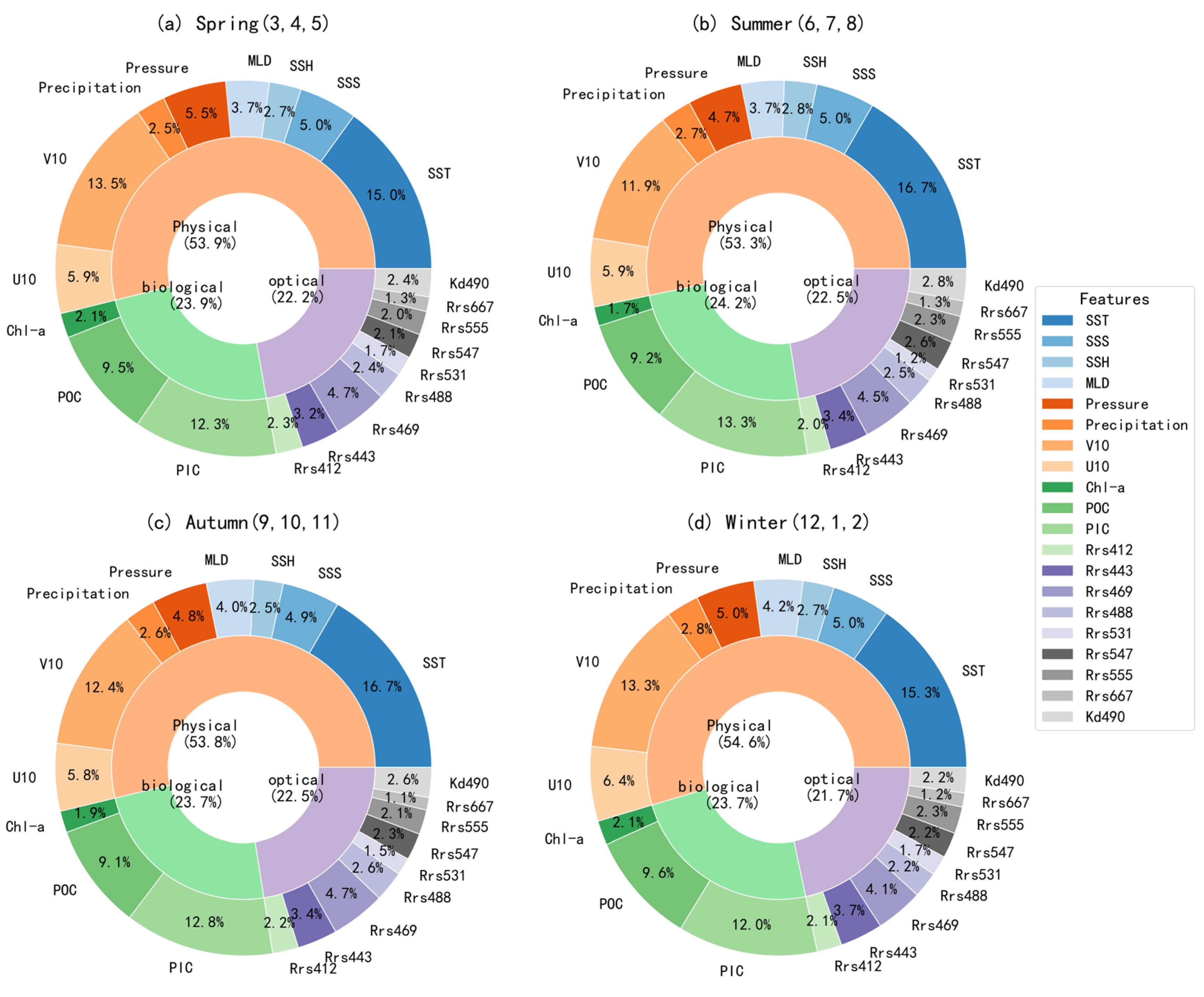
Figure 10 illustrates the seasonal variations in the relative contributions of different factors to surface pH predictions in the Pacific Ocean based on the XGBoost model. Overall, the relative contributions remained consistent across the four seasons. Physical factors consistently showed the highest contribution, ranging from 53.8% to 54.6%, highlighting the dominant role of physical processes in controlling surface pH variability. The contribution of biological factors was also stable, varying between 23.7% and 24.2%, while optical factors maintained a contribution between 21.9% and 22.3%. These results suggest that the key drivers influencing surface pH in the Pacific Ocean have no significant changes on seasonal scale.
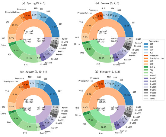
Figure 10.
The seasonal relative contributions of pH-influencing factors in the Pacific Ocean.
SHAP analysis identified SST, PIC, and POC as the primary factors influencing pH variability. This aligns with findings by Jiang et al. [16], who emphasized the role of biologically driven parameters such as POC and chlorophyll in shaping the surface carbonate system. However, our results provide more quantitative insights into their relative contributions (15.9% for SST, 12.6% for PIC, 9.4% for POC), which were not reported in such detail previously. Moreover, the strong sensitivity of pH to SST in the Niño 3.4 region corresponds with observations by Wu et al. [8], reinforcing the significance of ENSO-related processes. Therefore, further analysis regarding the contribution of pH-influencing factors in the ENSO region is provided in Section 4.2.
4.2. Analysis of pH Influencing Factors in the Niño 3.4 Region
Figure 11 shows the relative contributions of various influencing factors to surface pH predictions in the Niño 3.4 region of the Pacific Ocean. Overall, physical factors dominate this region, accounting for 51.1%, followed by biological factors at 31.7% and optical factors at 17.3%. Compared to the entire Pacific basin, the contribution of physical factors in the Niño 3.4 region is slightly lower (51.1% vs. 53.9%). In contrast, biological factors contribute significantly more (31.7% vs. 23.9%), while optical factors contribute slightly less (17.3% vs. 22.2%). These differences indicate that the mechanisms driving pH variability in the Niño 3.4 region are different from those operating across the broader Pacific Ocean.
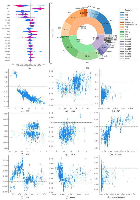
Figure 11.
(a,b) Summary of pH-influencing factors and their relative contributions in the Niño 3.4 region of the Pacific Ocean; (c–k) Dependence plots of major pH-influencing factors in the Niño 3.4 region of the Pacific Ocean.
The contribution of physical factors in the Niño 3.4 region remains comparable to that across the Pacific. However, in terms of biological factors, both PIC-related and POC-related processes contribute higher to pH dynamics in the Niño 3.4 region, accounting for 14.8% and 15.7%, respectively. Optical factors account for 17.3% in the Niño 3.4 region, reflecting a 4.9% decrease compared to the overall contribution in the Pacific. Rrs443 and Rrs469 continue to be the leading optical variables, contributing 2.9% and 4.3%, respectively.
In the Niño 3.4 region, SST shows a clearer negative correlation with pH compared with the whole Pacific, because the increase in temperature leads to a decrease in the solubility of CO2 and an increase in the dissociation of bicarbonate (HCO3−). This process results in the increased hydrogen ion (H+) concentrations and lower pH, which is particularly evident between 22 °C and 30 °C [30]. A related study has also indicated that ENSO can enhance OA, where the lower pH inhibited the deposition of POC (positive correlation) and aligned with the increase in PIC (negative correlation) [33]. Therefore, the positive/negative relationships of POC pH and PIC pH in the ENSO region are more evident, and their contribution is also greater.
5. Conclusions
This study proposed a spatiotemporal inversion framework for surface ocean pH based on interpretable machine learning, reconstructing high-resolution (8 km) pH distributions across the Pacific Ocean from 2003 to 2021. The spatiotemporal patterns and driving factors of OA were analyzed, revealing a clear latitudinal gradient and seasonal variability in pH. Persistent low pH values were observed in the equatorial Pacific and eastern Pacific upwelling regions, primarily due to the upwelling of CO2-enriched deep waters. In contrast, mid-to-high latitude regions showed relatively higher pH values influenced by major currents, such as the Kuroshio, Oyashio, and East Australian Current, as well as enhanced biological carbon fixation and physical mixing processes.
SHAP-based interpretability analysis identified SST as the predominant regulator of pH among all factors. In low-latitude warm regions, elevated SST promotes bicarbonate dissociation, increasing hydrogen ion concentration and lowering pH. At high latitudes, cooler temperatures enhance CO2 solubility, exacerbating acidification. In mid-latitudes, SST positively contributed to pH, potentially due to the downward transport of carbon in subtropical gyres, which mitigates acidification [27]. PIC negatively impacted pH by consuming alkalinity through biological calcification, while POC-forming processes such as biological carbon fixation reduced acidification, showing a positive contribution in most case regions.
Moreover, in the Niño 3.4 region, both PIC-related and POC-related processes displayed higher contributions to pH variability compared to the Pacific basin as a whole. This suggests that pH is more sensitive to particulate carbon-related biological processes in this area, indicating a potential pathway through which ENSO disturbances may affect pH by influencing PIC-related and/or POC-related processes. Therefore, the high-resolution pH dataset developed in this study serves as a valuable data-driven reference for understanding the mechanisms driving OA.
While data-driven approaches can integrate multi-source remote sensing observations and provide advantages in resolving fine-scale pH distributions and attributing the influence of physical, biological, and optical factors, OA is a complex and multidimensional process. Numerical modeling, which explicitly considers the interactions among carbonate system parameters, remains essential for a deeper mechanistic understanding. Nonetheless, this study offers important insights into the spatial and temporal dynamics of pH drivers. With the anticipated growth of observational networks, such as BGC-Argo and gliders, data-driven methods hold significant potential for the future quantitative exploration of OA driving factors, including atmospheric parameters, and algal species.
Author Contributions
Conceptualization, M.H., J.Q., Y.W. and S.W.; Methodology, M.H., J.Q., Y.W. and J.S.; Software, M.H., Y.C. and J.S.; Validation, C.Z. and Y.C.; Formal analysis, Y.W.; Investigation, C.Z. and Y.C.; Writing—original draft, M.H.; Writing—review & editing, J.Q. and C.Z.; Supervision, J.Q., Y.W. and S.W.; Funding acquisition, S.W. All authors have read and agreed to the published version of the manuscript.
Funding
This work was supported by the National Natural Science Foundation of China (grant 42406190), Fundamental Research Funds for the Central Universities (grant 226-2024-00124). This work was also supported by the Deep-time Digital Earth (DDE) Big Science Program and the Earth System Big Data Platform of the School of Earth Sciences, Zhejiang University.
Data Availability Statement
The data supporting reported results can be found in the following publicly available sources: SOCAT (https://socat.info/); ERA5 Reanalysis (https://cds.climate.copernicus.eu/datasets/reanalysis-era5-single-levels-monthly-means?tab=download); GLODAP (https://glodap.info/); NASA Ocean Color (https://oceancolor.gsfc.nasa.gov/); The Copernicus Marine Service (https://data.marine.copernicus.eu/product/GLOBAL_MULTIYEAR_PHY_001_030/download?dataset=cmems_mod_glo_phy_my_0.083_P1M-m).
Conflicts of Interest
The authors declare no conflict of interest.
Abbreviations
| Chl-a | Chlorophyll a |
| CO2 | Carbon Dioxide |
| Carbon Dioxide Fugacity | |
| R2 | Coefficient of Determination |
| DIC | Dissolved inorganic carbon |
| DOC | Dissolved organic carbon |
| XGBoost | EXtreme Gradient Boosting |
| ExtraTrees | Extremely Randomized Trees |
| ENSO | El Niño—Southern Oscillation |
| FFNN | feedforward neural network |
| GBDT | Gradient Boosting Decision Tree |
| GODAP | Global Ocean Data Analysis Project |
| LR | Logistic Regression |
| MAE | Mean Absolute Error |
| MLD | Mixed-Layer Depth |
| OA | Ocean Acidification |
| POC | Particulate Organic Carbon |
| PIC | Particulate Inorganic Carbon |
| pCO2 | partial pressure of carbon dioxide |
| RF | Random Forest |
| SST | Sea-surface Temperature |
| SSS | Sea-surface Salinity |
| SVR | Support Vector Regression |
| SSH | Sea-surface Height |
| SHAP | SHapley Additive exPlanations |
| SOCAT | The Surface Ocean Co2 Atlas |
| TA | Total Alkalinity |
References
- Siegenthaler, U.; Sarmiento, J.L. Atmospheric carbon dioxide and the ocean. Nature 1993, 365, 119–125. [Google Scholar] [CrossRef]
- Orr, J.C.; Fabry, V.J.; Aumont, O.; Bopp, L.; Doney, S.C.; Feely, R.A.; Gnanadesikan, A.; Gruber, N.; Ishida, A.; Joos, F.; et al. Anthropogenic ocean acidification over the twenty-first century and its impact on calcifying organisms. Nature 2005, 437, 681–686. [Google Scholar] [CrossRef] [PubMed]
- Ayache, N.; Lundholm, N.; Gai, F.; Hervé, F.; Amzil, Z.; Caruana, A. Impacts of ocean acidification on growth and toxin content of the marine diatoms Pseudo-nitzschia australis and P. fraudulenta. Mar. Environ. Res. 2021, 169, 105380. [Google Scholar] [CrossRef] [PubMed]
- Sabine, C.L.; Feely, R.A.; Gruber, N.; Key, R.M.; Lee, K.; Bullister, J.L.; Wanninkhof, R.; Wong, C.S.; Wallace, D.W.R.; Tilbrook, B.; et al. The Oceanic Sink for Anthropogenic CO2. Science 2004, 305, 367–371. [Google Scholar] [CrossRef]
- Feely, R.A.; Fabry, V.J.; Guinotte, J.M. Ocean acidification of the North Pacific Ocean. PICES Press 2008, 16, 22–26. [Google Scholar]
- Takahashi, T.; Sutherland, S.C.; Chipman, D.W.; Goddard, J.G.; Ho, C.; Newberger, T.; Sweeney, C.; Munro, D.R. Climatological distributions of pH, pCO2, total CO2, alkalinity, and CaCO3 saturation in the global surface ocean, and temporal changes at selected locations. Mar. Chem. 2014, 164, 95–125. [Google Scholar] [CrossRef]
- Landschützer, P.; Gruber, N.; Haumann, F.A.; Rödenbeck, C.; Bakker, D.C.E.; Van Heuven, S.; Hoppema, M.; Metzl, N.; Sweeney, C.; Takahashi, T.; et al. The reinvigoration of the Southern Ocean carbon sink. Science 2015, 349, 1221–1224. [Google Scholar] [CrossRef]
- Wu, H.C.; Dissard, D.; Douville, E.; Blamart, D.; Bordier, L.; Tribollet, A.; Le Cornec, F.; Pons-Branchu, E.; Dapoigny, A.; Lazareth, C.E. Surface ocean pH variations since 1689 CE and recent ocean acidification in the tropical South Pacific. Nat. Commun. 2018, 9, 2543. [Google Scholar] [CrossRef]
- Caldeira, K.; Wickett, M.E. Anthropogenic carbon and ocean pH. Nature 2003, 425, 365. [Google Scholar] [CrossRef]
- Gruber, N.; Hauri, C.; Lachkar, Z.; Loher, D.; Froelicher, T.L.; Plattner, G.-K. Rapid Progression of Ocean Acidification in the California Current System. Science 2012, 337, 220–223. [Google Scholar] [CrossRef]
- Feely, R.A.; Doney, S.C.; Cooley, S.R. Ocean acidification: Present conditions and future changes in a high-CO2 world. Oceanography 2009, 22, 36–47. [Google Scholar] [CrossRef]
- Wootton, J.T.; Pfister, C.A.; Forester, J.D. Dynamic patterns and ecological impacts of declining ocean pH in a high-resolution multi-year dataset. Proc. Natl. Acad. Sci. USA 2008, 105, 18848–18853. [Google Scholar] [CrossRef]
- Li, B.; Watanabe, Y.W.; Yamaguchi, A. Spatiotemporal distribution of seawater pH in the North Pacific subpolar region by using the parameterization technique. J. Geophys. Res.-Ocean. 2016, 121, 3435–3449. [Google Scholar] [CrossRef]
- Krishna, K.V.; Shanmugam, P.; Nagamani, P.V. A multiparametric nonlinear regression approach for the estimation of global surface ocean pCO2 using satellite oceanographic data. IEEE J. Sel. Top. Appl. Earth Obs. Remote Sens. 2020, 13, 6220–6235. [Google Scholar] [CrossRef]
- Iida, Y.; Takatani, Y.; Kojima, A.; Ishii, M. Global trends of ocean CO2 sink and ocean acidification: An observation-based reconstruction of surface ocean inorganic carbon variables. J. Oceanogr. 2021, 77, 323–358. [Google Scholar] [CrossRef]
- Jiang, Z.; Song, Z.; Bai, Y.; He, X.; Yu, S.; Zhang, S.; Gong, F. Remote Sensing of Global Sea Surface pH Based on Massive Underway Data and Machine Learning. Remote Sens. 2022, 14, 2366. [Google Scholar] [CrossRef]
- Zhong, G.; Li, X.; Song, J.; Qu, B.; Wang, F.; Wang, Y.; Zhang, B.; Cheng, L.; Ma, J.; Yuan, H.; et al. A global monthly 3D field of seawater pH over 3 decades: A machine learning approach. Earth Syst. Sci. Data 2025, 17, 719–740. [Google Scholar] [CrossRef]
- Nakano, Y.; Watanabe, Y.W. Reconstruction of pH in the Surface Seawater over the North Pacific Basin for All Seasons Using Temperature and Chlorophyll-a. J. Oceanogr. 2005, 61, 673–680. [Google Scholar] [CrossRef]
- Zeebe, R.E. History of Seawater Carbonate Chemistry, Atmospheric CO2, and Ocean Acidification. Annu. Rev. Earth Planet. Sci. 2012, 40, 141–165. [Google Scholar] [CrossRef]
- Lueker, T.J.; Dickson, A.G.; Keeling, C.D. Ocean pCO2 calculated from dissolved inorganic carbon, alkalinity, and equations for K1 and K2: Validation based on laboratory measurements of CO2 in gas and seawater at equilibrium. Mar. Chem. 2000, 70, 105–119. [Google Scholar] [CrossRef]
- Wallace, R.B.; Baumann, H.; Grear, J.S.; Aller, R.C.; Gobler, C.J. Coastal ocean acidification: The other eutrophication problem. Estuar. Coast. Shelf Sci. 2014, 148, 1–13. [Google Scholar] [CrossRef]
- Mattsdotter Björk, M.; Fransson, A.; Torstensson, A.; Chierici, M. Ocean acidification state in western Antarctic surface waters: Controls and interannual variability. Biogeosciences 2014, 11, 57–73. [Google Scholar] [CrossRef]
- Hauri, C.; Gruber, N.; Vogt, M.; Doney, S.C.; Feely, R.A.; Lachkar, Z.; Leinweber, A.; McDonnell, A.M.P.; Munnich, M.; Plattner, G.-K. Spatiotemporal variability and long-term trends of ocean acidification in the California Current System. Biogeosciences 2013, 10, 193–216. [Google Scholar] [CrossRef]
- Lauvset, S.K.; Lange, N.; Tanhua, T.; Bittig, H.C.; Olsen, A.; Kozyr, A.; Álvarez, M.; Azetsu-Scott, K.; Brown, P.J.; Carter, B.R.; et al. The annual update GLODAPv2.2023: The global interior ocean biogeochemical data product. Earth Syst. Sci. Data 2024, 16, 2047–2072. [Google Scholar] [CrossRef]
- Lauvset, S.K.; Lange, N.; Tanhua, T.; Bittig, H.C.; Olsen, A.; Kozyr, A.; Álvarez, M.; Becker, S.; Brown, P.J.; Carter, B.R.; et al. An updated version of the global interior ocean biogeochemical data product, GLODAPv2.2021. Earth Syst. Sci. Data 2021, 13, 5565–5589. [Google Scholar] [CrossRef]
- Lewis, E.; Wallace, D. Program Developed for CO2 System Calculations; Environmental System Science Data Infrastructure for a Virtual Ecosystem 1998; Oak Ridge National Lab., Carbon Dioxide Information Analysis Center: Oak Ridge, TN, USA.
- Li, X.; Gan, B.; Zhang, Z.; Cao, Z.; Qiu, B.; Chen, Z.; Wu, L. Oceanic uptake of CO2 enhanced by mesoscale eddies. Sci. Adv. 2025, 11, eadt4195. [Google Scholar] [CrossRef]
- Bates, N.; Astor, Y.; Church, M.; Currie, K.; Dore, J.; Gonaález-Dávila, M.; Lorenzoni, L.; Muller-Karger, F.; Olafsson, J.; Santa-Casiano, M. A Time-Series View of Changing Ocean Chemistry Due to Ocean Uptake of Anthropogenic CO2 and Ocean Acidification. Oceanography 2014, 27, 126–141. [Google Scholar] [CrossRef]
- Carter, B.R.; Feely, R.A.; Williams, N.L.; Dickson, A.G.; Fong, M.B.; Takeshita, Y. Updated methods for global locally interpolated estimation of alkalinity, pH, and nitrate. Limnol. Oceanogr. Methods 2018, 16, 119–131. [Google Scholar] [CrossRef]
- Jiang, L.-Q.; Carter, B.R.; Feely, R.A.; Lauvset, S.K.; Olsen, A. Surface ocean pH and buffer capacity: Past, present and future. Sci. Rep. 2019, 9, 18624. [Google Scholar] [CrossRef]
- Chan, F.; Barth, J.A.; Blanchette, C.A.; Byrne, R.H.; Chavez, F.; Cheriton, O.; Feely, R.A.; Friederich, G.; Gaylord, B.; Gouhier, T.; et al. Persistent spatial structuring of coastal ocean acidification in the california current system. Sci. Rep. 2017, 7, 2526. [Google Scholar] [CrossRef]
- Yu, J.; Wang, X.; Murtugudde, R.; Tian, F.; Zhang, R.-H. Interannual-to-decadal variations of particulate organic carbon and the contribution of phytoplankton in the tropical pacific during 1981-2016: A model study. J. Geophys. Res. Oceans. 2021, 126, e2020JC016515. [Google Scholar] [CrossRef]
- Chakraborty, K.; Joshi, A.P.; Ghoshal, P.K.; Baduru, B.; Valsala, V.; Sarma, V.V.S.S.; Metzl, N.; Gehlen, M.; Chevallier, F.; Lo Monaco, C. Indian ocean acidification and its driving mechanisms over the last four decades (1980–2019). Glob. Biogeochem. Cycles 2024, 38, e2024GB008139. [Google Scholar] [CrossRef]

Disclaimer/Publisher’s Note: The statements, opinions and data contained in all publications are solely those of the individual author(s) and contributor(s) and not of MDPI and/or the editor(s). MDPI and/or the editor(s) disclaim responsibility for any injury to people or property resulting from any ideas, methods, instructions or products referred to in the content. |
© 2025 by the authors. Licensee MDPI, Basel, Switzerland. This article is an open access article distributed under the terms and conditions of the Creative Commons Attribution (CC BY) license (https://creativecommons.org/licenses/by/4.0/).