Electrical Resistivity Tomography Methods and Technical Research for Hydrate-Based Carbon Sequestration

Abstract

This study focuses on the application of electrical resistivity tomography (ERT) for monitoring the growth process of CO₂ hydrate in subsea carbon sequestration, aiming to provide technical support for the safety assessment of marine carbon storage. By designing single-target, dual-target, and multi-target hydrate samples, convolutional neural networks (CNNs), recurrent neural networks (RNNs), and residual neural networks (ResNets) were constructed and compared with traditional image reconstruction algorithms (e.g., back-projection) to quantitatively analyze ERT imaging accuracy. The experiments used boundary voltage as the input and internal conductivity distribution as the output, employing the relative image error (RIE) and image correlation coefficient (ICC) to evaluate algorithmic performance. The results demonstrate that neural network algorithms—particularly RNNs—exhibit superior performance compared to traditional image reconstruction methods due to their strong noise resistance and nonlinear mapping capabilities. These algorithms significantly improve the edge clarity in target identification, enabling the precise capture of the hydrate distribution during carbon sequestration. This advancement effectively enhances the monitoring capability of CO₂ hydrate reservoir characteristics and provides reliable data support for the safety assessment of hydrate reservoirs.

1. Introduction

Natural gas hydrates (NGHs), also known as combustible ice, are non-stoichiometric ice-like crystalline compounds [1]. Various types of naturally occurring hydrates (CH₄, C₂H₆, CO₂, etc.) are primarily distributed at the edges of deep-sea continental shelves and in inland permafrost regions [2]. This distribution is determined by the phase equilibrium conditions for hydrate formation (low temperatures and high pressures) and geological environments (gas sources and water). Under standard conditions, one unit-volume of natural gas hydrate can decompose to produce up to one hundred sixty-four unit-volumes of methane gas. Calculations suggest that the reserves of methane and other gases stored in hydrate form in the natural world are twice the size of those of other fossil fuels [3]. Natural gas hydrates are viewed as an important alternative energy source in the 21st century due to their superior energy storage capabilities, driving the progress of marine combustible ice from small-scale trials to large-scale applications. In addition to being a high-quality replaceable energy source, natural gas hydrates play crucial roles in various energy and environmental industrial applications due to their unique physicochemical properties [4].

The stable existence of natural gas hydrates on the seafloor has been known for thousands of years, so researchers wonder whether CO₂ can also be stored long term beneath the seafloor, like CH₄ gas. The ocean provides a vast area for large-scale CO₂ sequestration. Theoretically, the storage of CO₂ hydrates is feasible, as the low-temperature and high-pressure conditions in the deep sea can create ideal conditions for the formation of CO₂ hydrates.

Currently, CO₂ in the form of hydrates is mainly stored in the seabed in two primary forms. The first form occurs when CO₂ is injected into deeper, high-pressure, and low-temperature sedimentary layers. As it migrates and diffuses, it combines with pore water in the sediments to generate solid CO₂ hydrates. This process further blocks the sediment pores, thereby forming self-sealing, non-permeable barriers [5,6]. The second form involves CO₂ displacing natural gas hydrates for extraction [7,8] or using artificial CO₂ hydrate caps to collaboratively extract natural gas hydrates [9]. The two types of hydrate carbon sequestration mechanisms are shown in Figure 1. This technology not only enhances the energy extraction of natural gas hydrates but also plays a role in maintaining the stability of the reservoir and the seabed’s geological structure [10].

Submarine CO₂ hydrates are typically hosted in porous geological media environments [12]. Their stability and formation mechanisms are influenced by factors such as the consolidation characteristics of reservoir rocks, permeability, and porosity [13]. These factors contribute to the complexity of CO₂ hydrate’s stability and formation mechanisms in submarine sediments. Lin et al. [14] conducted experimental and modeling studies, revealing that CO₂ injection induces adsorption-induced swelling in shale. This process alters the pore structure, increases the pore volume, and modifies the permeability while simultaneously weakening the mechanical properties of the shale. Consequently, it compromises the integrity and stability of the reservoir. In the study of the potential CO₂ storage site at Smeaheia, in the offshore Norwegian region, 3D field-scale geomechanical modeling based on seismic data indicates that the reservoir pressure increase induced by CO₂ injection can lead to significant vertical deformation (up to 8 cm) at the reservoir–caprock interface and the seabed surface. Additionally, the spatial variability of the overburden strata mitigates the risks of deformation localization and shear failure through stress redistribution, thereby reducing the likelihood of fault reactivation and subsequent CO₂ leakage [15]. Figure 2a illustrates the gradual increase in the reservoir pressure over a 50-year CO₂ injection period, with time steps delineated every 10 years. Figure 2b depicts the spatial distribution of the pressure, which is concentrated in the injection zone of the Vette–Øygarden fault block and constrained by the fault boundaries.

Non-homogeneous porous media are a critical factor in assessing the safety of seabed carbon storage. This understanding directly determines the safe and effective implementation of hydrate-based seabed carbon storage.

The formation of hydrates typically involves two stages: nucleation and crystal growth. In the nucleation stage, disordered or liquid-like molecules develop into a solid crystalline phase. In the crystal growth stage, as the particle size increases, the solid hydrate crystals gradually grow, as illustrated in Figure 3. Monitoring the hydrate formation process at a laboratory scale is an effective and low-cost method that can study the nucleation mechanisms of hydrates, providing theoretical support for in situ hydrate-based carbon sequestration. Currently, the main in situ visualization techniques commonly used in laboratory settings to monitor hydrate growth processes include computed tomography (CT), scanning electron microscopy, magnetic resonance imaging (MRI), and nuclear magnetic resonance (NMR). Zhang et al. utilized CT technology to measure hydrate growth processes and studied the relationship between the hydrate morphology and changes in permeability within the reservoir [16]. Simonetti et al. observed the microcrystalline structures of hydrate samples from different locations in the Gulf of Mexico, using scanning electron microscopy, and concluded that hydrates coexist with liquid oil [17]. Kuang et al. employed NMR to measure the in situ formation of CO₂ hydrates in porous media. They found that CO₂ hydrates predominantly form in larger pores, which further hinders gas–water contact in isolated pores during subsequent stages [18]. While these techniques can all be used to observe hydrate growth, they still have limitations. During the hydrate formation process, various material properties continually change, but the aforementioned technologies cannot satisfy the requirement for dynamic measurements of the hydrate growth process. As a result, they fail to effectively capture the instantaneous states of hydrate formation.

Electrical resistivity tomography (ERT) [20], an important branch of process tomography (PT) [21], operates on the principles of injecting a weak current into the target medium, measuring boundary voltages via surface electrodes, and combining finite element forward modeling with inverse problem reconstruction to generate cross-sectional images of the medium’s internal resistivity or conductivity distribution.

In terms of safety features, ERT technology, with its non-radiative and non-invasive characteristics, enables the long-term and repeated monitoring of sensitive marine geological environments, providing an ideal approach for the non-destructive observation of hydrate formation processes. Regarding resolution and dynamic capture capabilities, neural network models demonstrate sub-second temporal sampling and sub-centimeter spatial precision, allowing for the clear delineation of hydrate edge features. For adaptability to porous media and multi-target resolution, ERT combined with neural network technology exhibits superior performance over traditional algorithms in handling the diverse and complex morphologies of CO₂ hydrates within subsea sediments.

Although ERT has numerous advantages, its limitations, such as the restricted depth of penetration and lower sensitivity to high-resistivity targets, make it less effective in detecting deep permafrost and natural gas hydrates. Therefore, ERT is more suitable for use in combination with other geophysical methods (e.g., the transient electromagnetic method, TEM) to compensate for its shortcomings and achieve more comprehensive subsurface imaging [22].

Since 2014, resistivity tomography technology has gradually gained widespread attention from researchers in the field of hydrate formation dynamics. We have investigated and analyzed recent academic studies using ERT for hydrate imaging, as shown in

Table 1. Electrical resistivity tomography (ERT) technology’s recent research in the field of hydrate imaging.

Authors	Research Methods
Priegnitz et al., 2014 [23]	Three-dimensional electrical resistivity tomography is utilized to dynamically monitor the formation and dissociation processes of hydrates in a high-pressure low-temperature reservoir simulator (LARS). The measured data are subsequently processed using the inversion software tool Boundless to generate imaging results through inversion.
Li et al., 2020 [24]	Two-dimensional electrical resistivity tomography is used to monitor the formation process of hydrates in sandy sediments, and the ITS2000 industrial fault-scanning system is employed for imaging.
Zhao J. et al., 2022 [25]	Utilizing ERT technology, three-dimensional resistivity images of blocky and layered hydrates were established. It was found that the resistivity of blocky hydrates is significantly higher than that of layered hydrates, and their formation characteristics are influenced by the distribution of the pore water and the microstructure of hydrate pores.
Buddo et al., 2022 [22]	The integration of ERT with other geophysical methods, such as the transient electromagnetic method (TEM), improves the penetration depth and sensitivity to high-resistivity targets.
Liu et al., 2024 [26]	A cross-hole electrical resistivity tomography (CHERT) technique was designed to satisfy a wide range of resistivity measurements ranging from a few ohm-meters to thousands of ohm-meters, consistent with the resistivity responses of actual hydrate reservoirs.

.

Unlike the studies mentioned earlier, this paper focuses on the numerical modeling and algorithmic development for hydrate imaging in subsea reservoirs. The core contributions involve generating multi-morphology hydrate data through finite element simulations and enhancing electrical resistivity tomography (ERT) imaging’s accuracy by integrating neural network algorithms, thereby providing theoretical support for subsequent in situ monitoring technology development. Specifically, this study achieves innovations in the following aspects: 1. Modeling and Prediction: It simulates the growth state of gas hydrates in the reservoir and employs neural networks to predict ERT resistivity imaging. 2. Methodological Comparison: It utilizes technical approaches, such as the linear back-projection method and the conjugate gradient method, for ERT resistivity-imaging predictions, followed by a comparative analysis with the neural network method.

The findings demonstrate that the neural network method, when combined with ERT, offers robust technical support for microscopic hydrate imaging and generation dynamics research.

2. Experimental Theory

ERT is an advanced and widely used geophysical subsurface imaging technique, with applications in civil engineering, environmental surveys, hydrological exploration, mineral exploration, and archeology [27]; ERT has the advantage of being a low-cost, non-invasive geophysical method that allows for the rapid observation of subsurface resistivity variations over the entire length of a line or profile [28]. It can be used to determine the soil lithology, saturation levels, fracture zones, and the presence of groundwater [29].

The ERT system comprises three components: the sensor array, the data acquisition module, and the image reconstruction module, which determine the internal resistivity distribution of the measured object according to the boundary voltage data measured after the injection of a weak current, and visualize it on a computer. The basic principle of the system is shown in Figure 4.

In the ERT system, the computer control unit sends data acquisition commands to the data acquisition system. The data acquisition system applies current excitation to the sensor electrodes according to a specific pattern and transmits the measured voltage data to the data-processing unit for preprocessing. The processed data are then used as input for the image reconstruction algorithm, ultimately yielding a grayscale conductivity image of the object under testing.

In the ERT data acquisition system, there are two excitation modes: adjacent current injection and opposite current injection. The adjacent current injection mode ensures uniform information acquisition within the sensitive field and provides a moderate number of measured voltage values. Therefore, this study adopts the adjacent current injection mode. The operational principle of this mode is as follows: First, any pair of adjacent electrodes is selected as the starting point and current is injected into them. Next, the voltage signals at other adjacent electrodes are sequentially measured in a clockwise direction, excluding the electrodes immediately adjacent to the current-injecting pair. After completing a full cycle of measurements for all the electrodes, the next adjacent electrode pair in the clockwise direction is selected and the voltage measurement process is repeated until all the electrode pairs have been excited. Finally, the voltage dataset is saved to the computer. Assuming the number of electrodes is N, a total of N(N − 3)/2 independent voltage values can be obtained. In this study, the sensor employs 16 electrodes, and a single dataset comprises 108 voltage values.

3. Experimental Methods

3.1. Solution Methods for the ERT Forward Problem

The primary approaches for solving the ERT forward problem include analytical methods and numerical computation methods. The analytical methods require the establishment of an accurate field model to conduct theoretical derivations and solve the analytical expressions of the potential distribution within the field. However, this approach involves complex derivations and is only applicable to scenarios where the geometric configuration and medium distribution are highly uniform. It struggles to address non-uniform fields. Numerical computation methods, including the finite difference method (FDM), finite element method (FEM), boundary element method (BEM), and element-free Galerkin method (EFGM), are widely employed. In this study, the FEM is utilized to solve the forward problem of electrical resistivity tomography (ERT).

The variational principle serves as the theoretical foundation of the finite element method. Its core idea involves discretizing a continuous field into numerous small elements. Calculations are performed on these individual elements to establish local equations, which are then combined to form the global equation system of the original field. Solving this system yields discrete solutions for the continuous field. In this work, the FEM parameters for the sensitivity analysis include 16 electrodes and 1600 imaging pixels, as in Figure 5.

3.2. Solution Methods for the ERT Inverse Problem

The inverse problem of the ERT refers to the process of reconstructing the resistivity distribution of a region of interest by measuring its boundary voltage. The process is typically “ill-posed” and “nonlinear” [30] and is affected by many factors, such as the geometry of the electrodes and the electrical properties of the measurement target itself. Currently, methods to solve the ERT inverse problem include the linear back-projection (LBP) method [31], conjugate gradient method [32], as well as emerging neural-network-based algorithms [33,34,35], which have been widely used in imaging.

3.2.1. The Conjugate Gradient Algorithm [36]

The distribution of the boundary voltage and the medium resistivity in the sensitive field obtained by resistive tomography measurements is a nonlinear function. From the principle of the FEM in the positive problem’s solution above, it can be seen that the boundary voltage value of the sensitive field and the sensitivity can be approximately transformed to a linear relationship through finite element division, which is expressed by the matrix shown in Formula (1) as follows:

$$SG=Z$$

(1)

where S is an n × m-order sensitivity matrix, G is an m × 1-order resistivity vector matrix in the sensitive field, and Z is an n × 1-order boundary voltage vector matrix. The image reconstruction of the ERT is the solution of the G matrix, which is computed as follows using the conjugate gradient algorithm to solve the ERT inverse problem:

• Regularization of the sensitivity matrix. The sensitivity matrix calculated above is not a symmetric positive definite matrix, so its transpose (S^T) at both ends of the formula should be multiplied simultaneously in order to convert the coefficient matrix to a symmetric positive definite matrix; otherwise, the conjugate gradient algorithm cannot converge. The regularization of the sensitivity matrix yields Formula (2) as follows:

$$S^{T}SG=S^{T}Z$$

(2)

By making A = S^TS, x = G, and b = S^TZ, Equation (2) can be transformed to the calculation of the linear equation Ax = b.

2.

Iterative calculation. In accordance with the principle of calculating the conjugate gradient above, for any initial value of x₀, the first iteration of the direction of $r_0=b-A_{X_0},p_0=r_0$ and then the directions of the subsequent conjugate gradients are, in turn, iteratively calculated in accordance with Formulas (3)–(7) as follows:

$${\alpha }_k={\displaystyle \frac{\left(r_k,r_k\right)}{\left(A_{P_k},p_k\right)}}$$

(3)

$$x_{k+1}=x_k+{\alpha }_k{p}_k$$

(4)

$$r_{k+1}=r_k-{\alpha }_{k}A{p}_k$$

(5)

$${\beta }_k={\displaystyle \frac{\left(r_{k+1},r_{k+1}\right)}{\left(r_k,r_k\right)}}$$

(6)

$$p_{k+1}=r_{k+1}-{\beta }_k{p}_k$$

(7)

Among them, P_k represents the direction of the kth iteration, and each iteration direction directly satisfies the conjugate relationship, as shown in Formula (8):

$$\left(p_i,A{p}_j\right)=0, i\ne j$$

(8)

After several iterations, the residuals are less than the set value, at which point the iteration is terminated and the optimal solution is found.

3.2.2. The Back-Projection Method

The inverse problem in resistive tomography is typically an ill-posed problem, where small perturbations in the measured boundary voltages can lead to significant changes in the reconstructed grayscale estimates of the image. Therefore, regularization methods are usually used to stabilize the solution of the inverse problem. Common regularization methods include least squares and Tikhonov regularization.

The reconstruction process of resistive tomography often needs to be solved using numerical methods, such as iterative methods and filtered back-projection (FBP). Filtered back-projection combines filtering techniques to effectively reduce the blurring effect in simple back-projection.

The goal of the ERT is to recover the resistivity, $\sigma \left(x,y\right)$, from known voltage data, $P\left(\theta ,t\right)$, the process of which can be represented by the following back-projection equation, as shown in Formula (9):

$${\sigma }_{rc}\left(x,y\right)={\int }_0^{\pi }P\left(\theta ,x\mathit{cos}\theta +y\mathit{sin}\theta \right)d\theta$$

(9)

In resistive tomography, $P\left(\theta ,t\right)$ represents the projection data for the voltage, while $\sigma \left(x,y\right)$ represents the resistivity distribution. θ is the angle of the electrode pair, and t is the projection path associated with the electrode array.

• The difference between the actual measured voltage and the background voltage. The actual measured voltage is $V_{ij}^{measured}$, and the background voltage ($V_{ij}^{measured}$) is calculated from the forward model. The voltage difference is shown in Formula (10) as follows:

  $$\Delta V_{ij}=V_{ij}^{measured}-V_{ij}^{background}$$

  (10)
• Constructing the sensitivity matrix and voltage difference vector. The sensitivity matrix (S) is arranged in two dimensions, with rows corresponding to the measurement pairs (i,j) and columns corresponding to the pixels (k). The voltage difference ($\Delta V$) is organized as a vector.
• Using inverse projection to calculate the conductivity change. The resistivity change ($\Delta \sigma$) is obtained by multiplying the sensitivity matrix’s transpose with the voltage difference, as shown in Formula (11):

  $$\Delta \sigma =S^T\Delta V$$

  (11)
  That is, the amount of the change per pixel k is shown in Formula (12) as follows:

  $$\Delta {\sigma }_k=\sum _{i,j}{S}_{ijk}\Delta V_{ij}$$

  (12)
• Normalization. Normalization to $\Delta {\sigma }_k$ is carried out as shown in Formula (13):

  $$\Delta {\sigma }_k^{norm}={\displaystyle \frac{\Delta {\sigma }_k}{{\Sigma }_{ij}\left|S_{ijk}\right|+\epsilon }}$$

  (13)

  where $\epsilon$ is a small constant to avoid dividing by zero.
• The reconstruction of the result output. The $\Delta \sigma$ value is output as a resistivity change image.

3.2.3. Neural Network Methods

The Preparation of the Training Dataset

In this work, a voltage–conductivity dataset was designed using the EIDORS software platform (EIDORS 3.8) [37] to simulate the gas hydrate generation situation in an autoclave.

In the preparation of the training dataset, we have comprehensively considered the natural occurrence states of gas hydrates within reservoirs. Based on their morphological characteristics, gas hydrates can be classified into five occurrence modes: blocky, nodular, layered, vein-like, and dispersed. According to their filling mechanisms, they are further categorized into five types: contact type, cementation type, pore-filling type, supporting type (or bridging type), and plaque type, as illustrated in Figure 6. Building on this framework, this study systematically accounts for diverse gas hydrate occurrence patterns. We established two primary categories of samples based on their dominant occurrence modes: (1) blocky/nodular gas hydrate models and (2) layered/vein-like gas hydrate models, as depicted in Figure 7 and Figure 8.

(1)

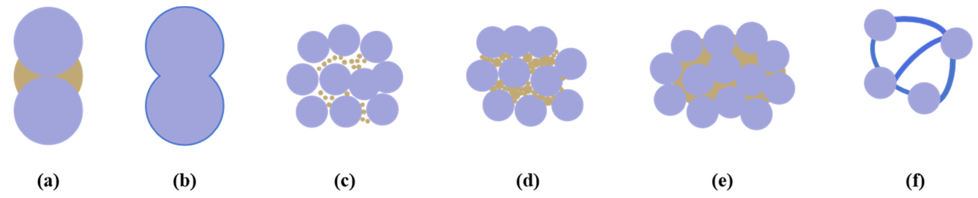
Blocky or Nodular Hydrate Model:

Blocky and nodular hydrates are large-scale gas hydrate structures characterized by blocky and nodular morphologies, often with minor sand grain inclusions. These features are exemplified by the hydrate deposits identified in China’s Shenhu Area [40], as illustrated in Figure 7.

(2)

Layered or Vein-type Hydrate Model:

Layered and vein-type hydrates refer to hydrate formations that grow within fractures, primarily found in inland seas and permafrost regions, such as the permanent permafrost layer of the Qilian Mountains in China [41]. This type of hydrate generally has a smaller shape and often exhibits irregular shapes during formation. In response to this, we designed simulated samples by adjusting the positions and numbers of high-resistance objects (hydrates) in the model, as shown in Figure 8.

Because neural network training requires large-scale datasets, we generated 14,508 sets of data by varying the size and location of the generated heterogeneous bodies. The number of each type of data is shown in

Table 2. Two-dimensional ERT voltage–resistivity simulation dataset distribution.

Sample Type	One Heterostructure	Two Heterostructures	Three Heterostructures	Four Heterostructures	Five Heterostructures
Training Sample	3000	3000	2000	3000	3000
Validation Sample	100	100	100	100	100
Testing Sample	1	1	1	1	1

.

Because there are certain differences between the simulated and measured datasets, which, to some extent, affect the performance capability of the neural network model in the measured dataset, we carried out a normalization operation on the voltage data in the simulated dataset and used the normalized voltage data for model training. The data normalization formula is expressed as shown in Formula (14):

$$x^{*}={\displaystyle \frac{x-x_{min}}{x_{max}-x_{min}}}$$

(14)

3.2.4. Network Algorithms and Models

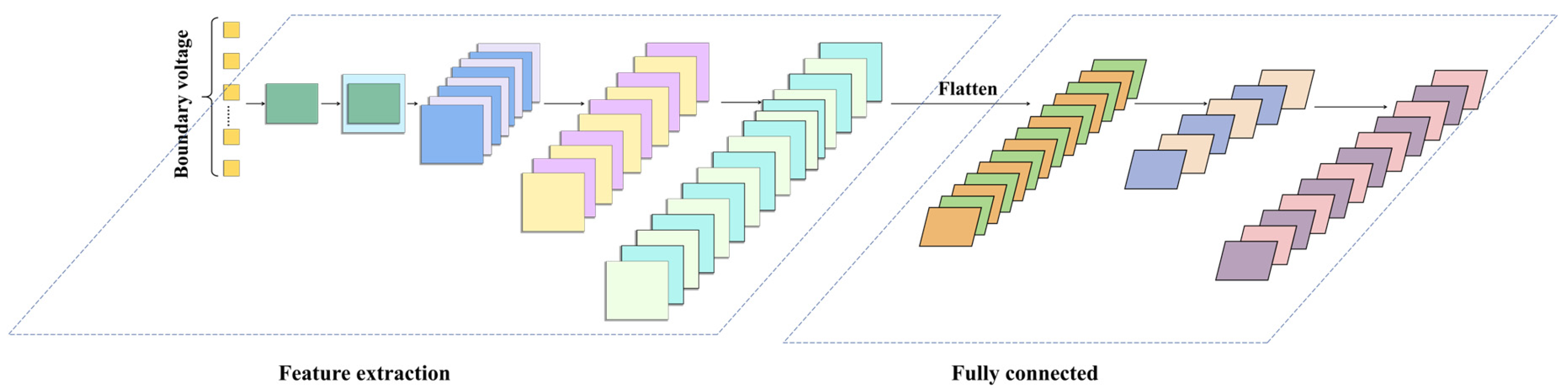
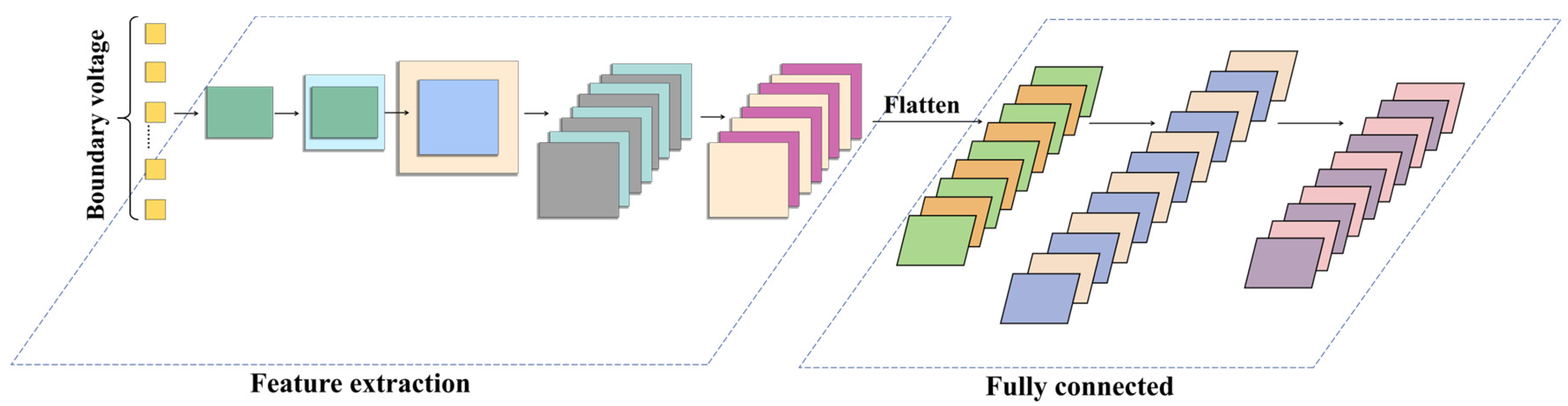
• CNN1

Because CNNs are suitable for processing image data, and the collected data in this work are measured voltage data, which do not match the shape of the picture data, before the data were input into the model, the data’s shape was transformed. The original sequence of 1 × 208 (as a 13 × 16 matrix) was zero-padded (Zero Padding), and the output was turned into a matrix of (18, 18, 1). Then, three convolutional operations were carried out using 8, 16, and 32 convolutional filters of a size of 3 × 3 and a step size of 1, and after each convolution, after the BN (batch normalization) layer on the feature map, to enhance the stability of the model. After the convolution, the shape of the output data was 18 × 18 × 256. Because the final number of prediction results for the internal conductivity was 1600, in this paper, the flattened layer and fully connected layer were used to pass through the data after the convolution; after flattening, the data shape was converted to (1, 82, 944), and further, after one fully connected layer with 512 neurons, the data shape was converted to (1512). After going through the last fully connected layer with 1600 neurons, the data shape was converted to (1, 1600). Because in this study, the prediction is for the presence or absence of hydrate as a 0−1 binary classification problem, after the last fully connected layer, a sigmoid function is used as the activation function for the output layer to map the 1600 input values between 0 and 1. The changes in the dimensions of the data matrix throughout this process are detailed in

Table 3. The changes in the dimensions of the data matrix throughout this process.

Step	Layer(s)	Output Size
Input	Reshaping + Zero Padding	(1, 18, 18, 1)
1	Conv2d/BN	(1, 18, 18, 64)
2	Conv2d/BN	(1, 18, 18, 256)
3	Conv2d/BN	(1, 2000)
4	Flattening	(1, 82, 944)
5	Fully connected	(1, 512)
6	Fully connected	(1, 1600)

.

The CNN architecture used in this paper is shown in Figure 9.

2.

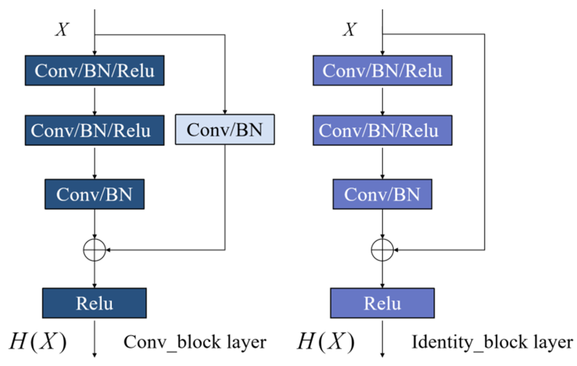
ResNet2

Compared with the convergence speeds of CNNs and other model architectures, those of the ResNet network are faster, and at the same time, it is beneficial to alleviate the problem of the gradient’s instability. Based on the deep residual network, a single-input, dual-output “h-Net” model architecture was designed [42], which can simultaneously achieve manifold discrimination and Electrical Resistivity Tomography (ERT) imaging. In this paper, targeting the imaging problem of saturated layer reservoirs, the “h-Net” model was simplified, and the simplified model was trained on sample data. He et al. proposed two base residual modules in ResNet50, Conv_block and Identity_block (as shown in Figure 10), which have the following model structure [43]:

As in the case of predictions using CNN models, in this paper, the original sequence was first subjected to a shape transformation and a complementary zero operation so that the shape of the data was changed to (1, 18, 18, 1); Following this, the data passed through a convolutional layer with 16 filters and astride of 2, followed by a Batch Normalization (BN) layer, resulting in an output shape of (1, 17, 17, 16). This output is then fed into a Conv_block layer, which main-tains the data shape without any changes. Next, the data undergoes flattening and is processed by a fully connected layer with 1800 neurons. A Dropout layer is applied afterward, followed by another fully connected layer with 1600 neurons. Finally, a Sigmoid activation function is used to map the output values to the range [0, 1], producing the final prediction. Based on the ResNet network, the model structure in this paper is as shown in Figure 11.

The changes in the dimensions of the data matrix throughout this process are detailed in

Table 4. The changes in the dimensions of the data matrix throughout this process.

Step	Layer(s)	Output Size
Input	Reshaping + Zero Padding + Upsampling/BN	(1, 36, 36, 1)
1	Conv2d/BN	(1, 17, 17, 16)
2	Conv_block layer/BN	(1, 17, 17, 16)
3	Flattening	(1, 4624)
5	Fully connected	(1, 1800)
6	Fully connected	(1, 1600)

.

3.

RNN3

Unlike CNNs, RNNs are more suitable for processing sequence-based data and have been used in bioinformatics to analyze bioinformatic sequences, such as DNA, RNA, and proteins [44]. For example, Li et al. utilized RNNs for gene prediction and protein structure prediction, demonstrating the ability of RNNs to capture dependency relationships in biological sequences and providing insights into genetic information and biological processes [45]. In this study, the input data comprise boundary voltage sequences, and the output data correspond to resistivity sequences. To compare the predictive performances of the RNN, CNN, and ResNet while enhancing the prediction accuracy, we employ the RNN for resistivity image reconstruction.

The input to the network consists of voltage measurement sequences, requiring no additional shape transformation. That is, the sequence of the input network is (208, 1), which first passes through an RNN layer with 16 neurons, at which point the sequence shape is (208, 16). Thereafter, the output sequence is paved and passes through the first fully connected layer with 1024 neuron nodes, at which point the output is (1024, 1). After this, 30% of the neurons are discarded to prevent possible overfitting, and, finally, a fully connected neural network with 1600 neuron nodes is used and activated with a sigmoid function to make the output data shape (1, 1600). The changes in the dimensions of the data matrix throughout this process are detailed in

Table 5. Changes in the dimensions of the data matrix throughout this process.

Step	Layer	Output Size
Input	——	(208, 1)
1	RNN × 16	(208, 16)
2	Flattening	(1, 3328)
3	Fully connected	(1, 2000)
4	Fully connected	(1, 1600)

.

The RNN architecture used in this paper is shown in Figure 12 below.

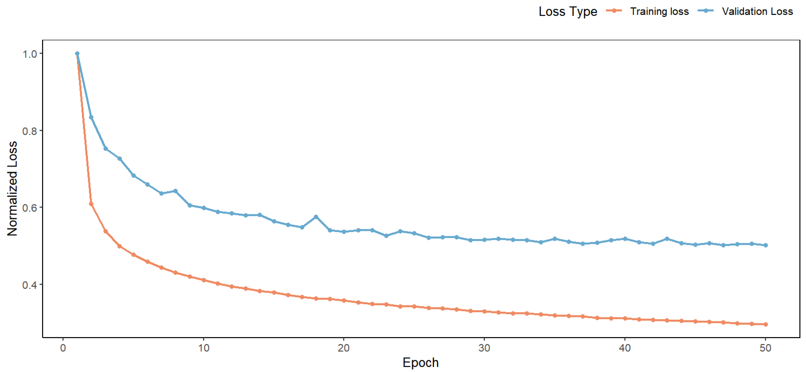
3.2.5. Network-Training-Related Parameter Settings

The computer operating system used for the experiment is Windows 11, the memory is 16 GB, the training framework used is TensorFlow 2.15, and the loss function used in the model compilation is the binary cross-entropy function, which portrays the distance between two probability distributions. The lower the cross-entropy is, the closer the two function distributions are, which is applicable to the binary classification problem. The function’s expression is shown in Formula (15) as follows:

$$binary\_crossentro py(Y^{pred},Y^{true})={\displaystyle \frac{1}{N}}\sum _{i=1}^N(Y_i^{true}\mathit{log}(Y_i^{pred})+(1-Y_i^{true})\mathit{log}(1-Y_i^{pred}))$$

(15)

Adaptive moment estimation (Adam) is one of the most commonly used optimization algorithms, which combines the advantages of the AdaGrad and RMSProp methods and is able to generate adaptive learning rates for different parameters in the model. At the same time, updating of the parameters is not affected by the scalar transformation of the gradient, and because the updating step is independent of the gradient size, this ensures robust convergence during optimization. Adam is able to better handle noisy samples and is suitable for tasks with large-scale data and parameters. Therefore, in this paper, we use Adam as the optimizer of the loss function and set the initial learning rate to 0.001.

The detailed metrics for each of the neural network trainings performed in this paper are shown in

Table 6. Neural network training configurations in this paper.

Computer Operating System	Windows 11
Training framework	Keras
Number of training samples	14,000
Number of calibration samples	500
Batch_size	64
Learning rate	0.01
Total training rounds	50
Loss function	Binary cross-entropy

.

The loss variations in the above three models during the training process are shown in Figure 13, Figure 14 and Figure 15.

From the loss changes in the three models (as shown in Figure 13, Figure 14 and Figure 15), it can be seen that for the loss values of the three models in the training process, the training set and the calibration set data show a converging trend, and there is no noticeable increase. This indicates that the three models perform better on the training set data and that the models do not appear to exhibit the overfitting phenomenon.

3.3. Model Evaluation Indicators

The image reconstruction quality’s evaluation criteria in this paper are the relative image error (RIE) and the image correlation coefficient (ICC), as shown in Equations (16) and (17):

$$RIE={\displaystyle \frac{{‖y^{*}-y‖}_2}{{‖y‖}_2}}$$

(16)

$$ICC={\displaystyle \frac{cov\left(y^{*},y\right)}{\sqrt{var\left(y^{*}\right)var\left(y\right)}}}$$

(17)

where $y^{*}$ and y are the estimated conductivity sequence and target conductivity sequence, respectively, and $cov( )$ and $var( )$ denote the covariance and mean-square deviation, respectively. The higher the ICC value is, the higher the correlation between the reconstructed image and the target image [46].

The lower the RIE value is, the more similar the reconstructed image is to the target image.

4. Results and Discussion

This study models the growth dynamics of CO₂ hydrates in reservoir environments and applies neural-network-based image reconstruction to characterize their spatial distributions. Simulated test samples, featuring circular heterogeneous bodies with variable sizes, quantities, and positions, were generated using EIDORS software(EIDORS 3.8). Both a neural network algorithm and a conventional reconstruction method were employed to predict electrical conductivity distributions, after which their performances were systematically compared across different target configurations, including varying body sizes and numbers.

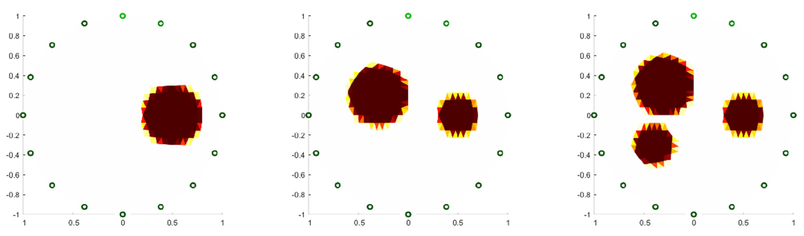
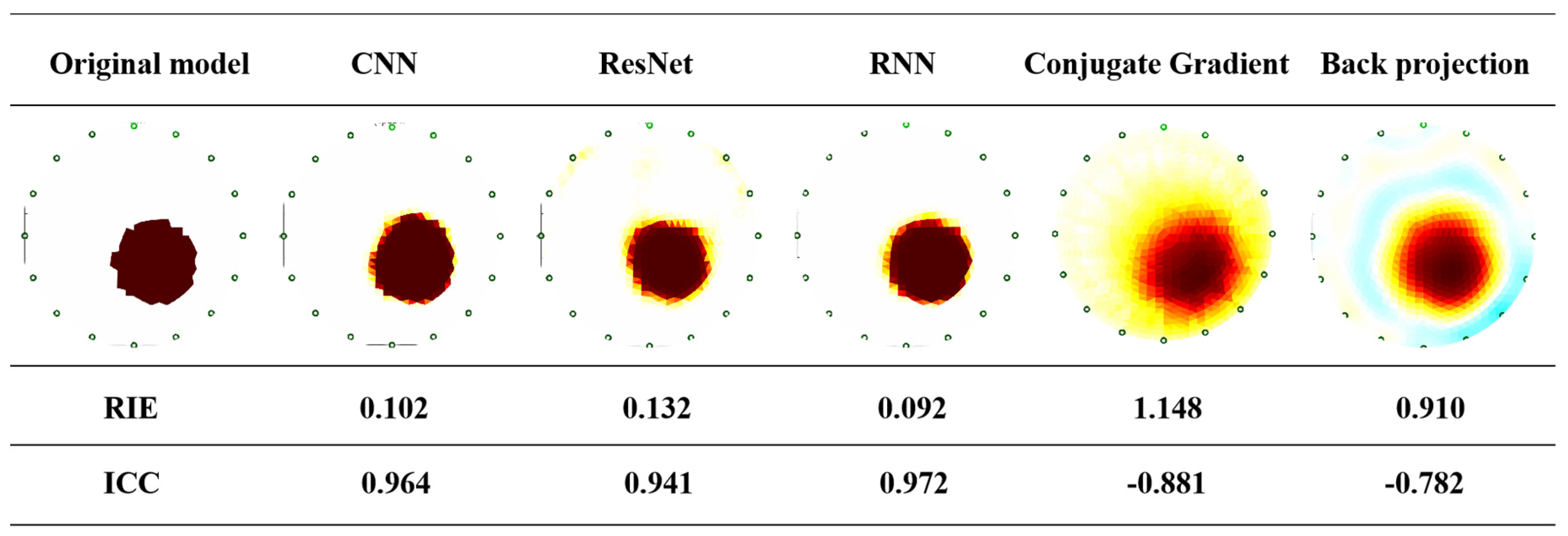
4.1. Comparison of Neural Networks and Traditional Image Reconstruction Algorithms for Recognizing a Single-Target Body

In comparing the accuracies of different algorithms for single-target recognition, the original single-target model is a good conductor located in the lower right corner. The imaging results and various metrics for the different image reconstruction algorithms are shown in Figure 16.

The relative image errors (RIEs) of traditional image reconstruction algorithms are significantly higher than those of the neural network method, and RNN-FCNN shows the maximum and minimum values of the RIE, indicating that RNN-FCNN has a significant advantage in image reconstruction. For the image correlation coefficient (ICC), RNN-FCNN and the conjugate gradient method show the maximum and minimum ICC values, respectively, which indicates that RNN-FCNN is more capable of maintaining the image quality, whereas image reconstruction algorithms, such as the conjugate gradient method, with ICC values below 0, are still deficient in image recognition tasks.

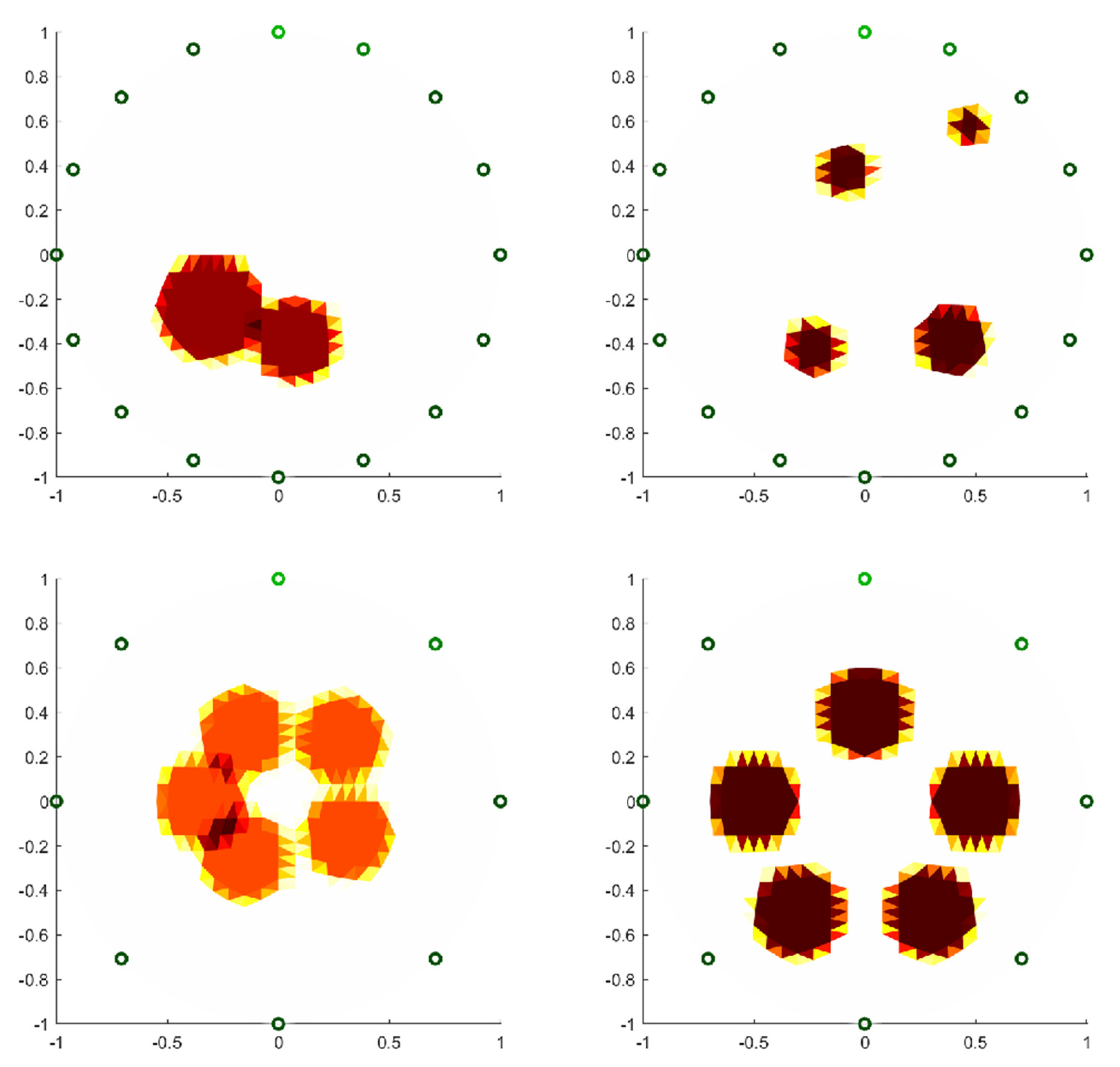
4.2. Comparison of Recognition Performances Between Neural Networks and Traditional Image Reconstruction Algorithms for Multiple Objects

By varying the number of and distance between heterogeneities, we generated dual-heterogeneity samples at different distances, as well as triple- and quintuple-heterogeneity samples. Among these, the recognition performances of the different imaging algorithms for the dual-heterogeneity samples at varying distances are shown in Figure 17.

The analysis of the experimental results shows that various types of image reconstruction algorithms exhibit significant distance correlations when dealing with heterogeneous bodies. Specifically, the algorithms as a whole show higher ICC values and lower RIE values when the heterogeneous bodies are farther apart, while they show lower ICC values and higher RIE values when the heterogeneous bodies are closer together. This indicates that the spatial resolution of the heterogeneous bodies directly affects the accuracy of the target recognition, and the variation in the spacing plays an important role in the quality of the image reconstruction.

When comparing the neural-network-based image reconstruction algorithms with the traditional image reconstruction algorithms, a notable conclusion is that even under the challenging condition of the close spacing of the heterogeneous bodies, the neural network method still exhibits lower RIE values and higher ICC values, demonstrating greater robustness and adaptability. Among them, the overall performance of the RNN-FCNN model is the most prominent, and this model outperforms the other algorithms.

Next, we analyzed the recognition performances of the different image reconstruction algorithms for the triple- and quintuple-heterogeneity targets; the imaging and metric calculation results are shown in Figure 18.

Analyzing the above results, the neural-network-based algorithms perform well in terms of the RIE in the multi-target recognition task and maintain a low overall level. Among them, the RNN-FCNN model performs the best, with the lowest RIE value. In contrast, the RIE value of the traditional algorithm is about ten times that of the neural network method, which is significantly higher than the latter. In terms of the ICC, the neural network method also generally outperforms the traditional image reconstruction algorithms, among which the RNN-FNCC model has the highest average ICC value, demonstrating excellent image reconstruction quality.

In summary, the following conclusions can be drawn: (1) All the image reconstruction algorithms show the optimal reconstruction performance, i.e., the highest ICC value and the lowest RIE value, in single-target detection scenarios. (2) Compared with the traditional image reconstruction algorithms, the neural network image reconstruction algorithms show better overall performances, especially in the case of the close proximity of heterogeneous bodies and irregular shapes, with a generally higher ICC value and a lower RIE value. (3) Among the neural network algorithms, the RNN model has the most outstanding performance; whether in single-target, dual-target, or multi-target reconstruction tasks, its ICC value can reach more than 0.85, and its RIE value is the lowest, which fully proves that the RNN model has the highest reconstruction accuracy and the most stable performance in image reconstruction tasks.

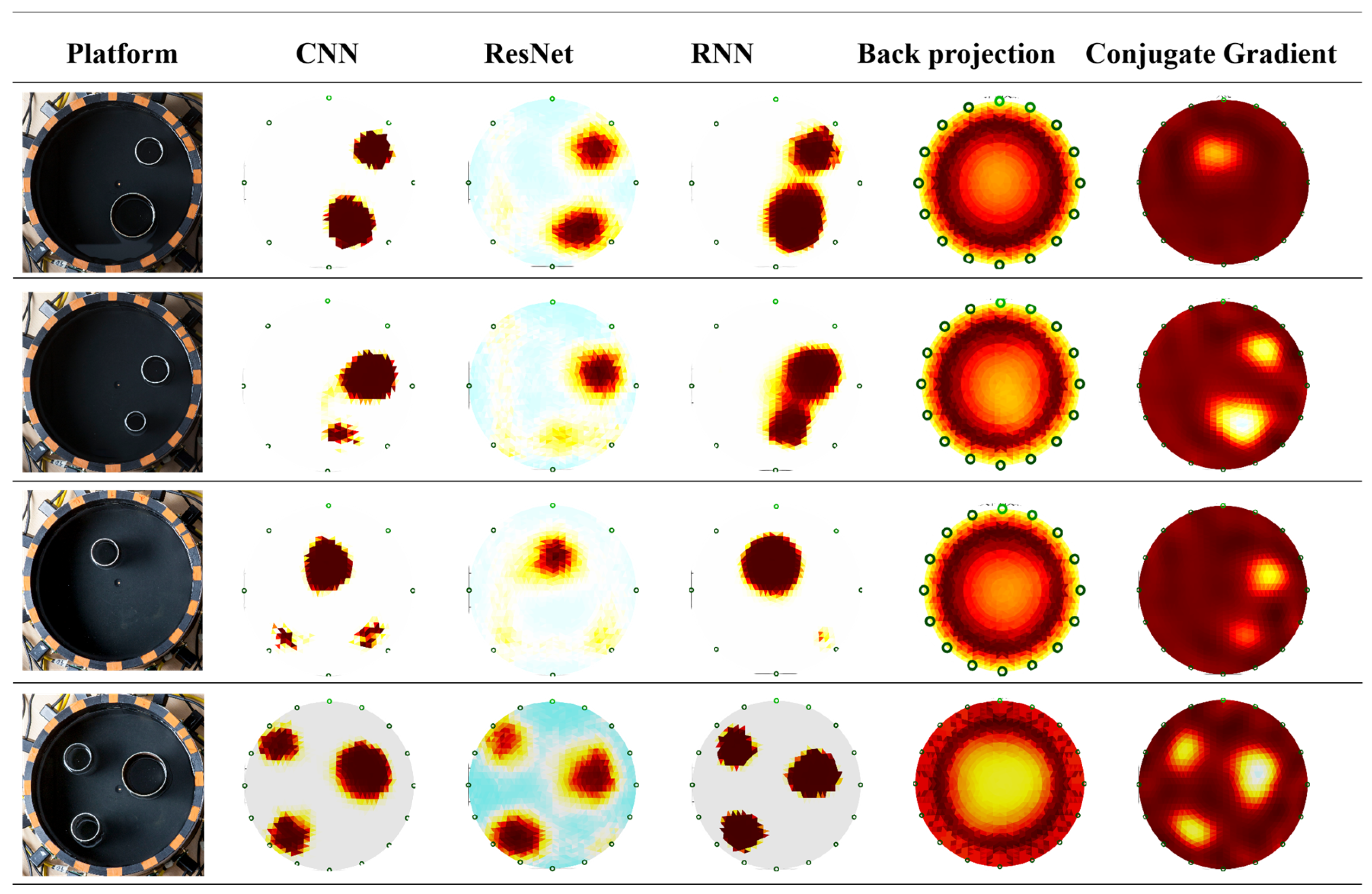
4.3. Phantom Experiment

To further test the performance of the neural-network-based image reconstruction, this study uses data acquired from the Kuopio electrical impedance tomography device (KIT4) [41] to evaluate the trained network.

The KIT4 EIT system was developed by the University of Eastern Finland (UEF). The voltage-controlled current source operates at 15 kHz, with an output impedance of up to 17 MΩ. During long-term experiments, the KIT4 system achieved a signal-to-noise ratio (SNR) of up to 97.5 dB, which is relatively high.

The boundary voltages measured using the KIT4 system were used as input to the network model to predict the conductivity distribution and reconstruct the image. The imaging performances of the conjugate gradient method and the back-projection method were compared with that of the neural network method, as shown in Figure 19.

The results show that the neural network model trained using the simulated dataset is able to correctly identify the shape and position of the target metal object in the KIT4 dataset, and the model has better generalization. Meanwhile, compared with the imaging effect of the traditional algorithm, the neural network imaging results have clearer edge contours, fewer artifacts, and higher imaging quality. Therefore, the neural network image reconstruction algorithm proposed in this paper is capable of the real-time monitoring and imaging of detection targets in different industrial tasks.

5. Conclusions

This study aimed to enhance the precision of electrical resistivity tomography (ERT)-based image reconstruction, providing a novel and effective solution for imaging the growth process of CO₂ hydrates in laboratory experiments. By systematically comparing various ERT image reconstruction algorithms, including traditional iterative methods, back-projection methods, and emerging neural network algorithms, the research evaluated their imaging performances based on key metrics. The goal was to identify algorithms with superior performances and propose optimization recommendations to address their limitations. This will enable ERT technology to provide more reliable and efficient solutions for the dynamic imaging of gas hydrate formation at the microscale. Using both simulated datasets and the KIT4 experimental dataset for sample-imaging analysis, the following conclusions were drawn: 1. Neural network models outperform traditional image reconstruction algorithms in terms of imaging accuracy and reduced artifacts. The neural-network-based image reconstruction algorithm significantly improves the issues of multiple artifacts and blurred edges present in traditional ERT-imaging algorithms, thereby enhancing the quality of the reconstructed images. Compared to traditional algorithms, neural network algorithms show significant advantages in key metrics, such as RIE and ICC, particularly in multi-target recognition tasks, where neural networks are more precise in identifying target positions and sizes. 2. Compared to CNN and ResNet, RNN performs the best, with the highest image reconstruction quality. In the tasks involving different numbers of targets, RNN consistently achieves ICC values of 0.85 or higher and the lowest RIE values, while ResNet exhibits relatively poor imaging performance, with lighter artifacts in the backgrounds of sample images from the KIT dataset.

Based on the comprehensive analysis, future research will focus on the following directions:

• Designing a multi-electrode seabed simulation system based on ERT to measure dynamic data of hydrate formation.
  Design and assemble a multi-layer reactor suitable for ERT research, with embedded electrode plates for voltage measurements during hydrate formation, providing a data foundation for ERT imaging.
• Advancing ERT technology from 2D to 3D.
  By adjusting electrode placements, optimizing algorithmic structures, and developing more precise 3D ERT technology, the system can process large amounts of data more efficiently and generate high-precision resistivity distribution images.
• Exploring fusion strategies between neural networks and traditional image reconstruction algorithms.
  Using the results of traditional algorithms as input to neural networks, this study aims to leverage the prior information of traditional algorithms to enhance the learning capabilities of neural networks, thereby improving the model’s generalization and robustness across different experimental datasets.

References

- Wei, N.; Pei, J.; Li, H.; Zhou, S.; Zhao, J.; Kvamme, B.; Coffin, R.B.; Zhang, L.; Zhang, Y.; Xue, J. Classification of natural gas hydrate resources: Review, application and prospect. Gas Sci. Eng. 2024, 124, 205269. [Google Scholar] [CrossRef]
- Sloan, E.D. Fundamental principles and applications of natural gas hydrates. Nature 2003, 426, 353–359. [Google Scholar] [CrossRef] [PubMed]
- Suess, E.; Torres, M.E.; Bohrmann, G.; Collier, R.W.; Rickert, D.; Goldfinger, C.; Linke, P.; Heuser, A.; Sahling, H.; Heeschen, K.; et al. Sea Floor Methane Hydrates at Hydrate Ridge, Cascadia Margin. In Natural Gas Hydrates: Occurrence, Distribution, and Detection; AGU Publications: Washington, DC, USA, 2001; pp. 87–98. [Google Scholar]
- Song, Y.; Yang, L.; Yang, M. Natural gas hydrate, far beyond a vast resource of natural gas. Innov. Energy 2025, 2, 100074. [Google Scholar] [CrossRef]
- Teng, Y.; Zhang, D. Long-term viability of carbon sequestration in deep-sea sediments. Sci. Adv. 2018, 4, eaao6588. [Google Scholar] [CrossRef]
- White, C.M.; Strazisar, B.R.; Granite, E.; Hoffman, J.S.; Pennline, H.W. Separation and Capture of CO2 from Large Stationary Sources and Sequestration in Geological Formations—Coalbeds and Deep Saline Aquifers. J. Air Waste Manag. Assoc. 2003, 53, 645–715. [Google Scholar] [CrossRef]
- Li, M.; Rojas Zuniga, A.; Stanwix, P.L.; Aman, Z.M.; May, E.F.; Johns, M.L. Insights into CO2-CH4 hydrate exchange in porous media using magnetic resonance. Fuel 2022, 312, 122830. [Google Scholar] [CrossRef]
- Zhang, L.; Yang, L.; Wang, J.; Zhao, J.; Dong, H.; Yang, M.; Liu, Y.; Song, Y. Enhanced CH4 recovery and CO2 storage via thermal stimulation in the CH4/CO2 replacement of methane hydrate. Chem. Eng. J. 2017, 308, 40–49. [Google Scholar] [CrossRef]
- Sun, L.; Meng, X.; Wang, J.; Li, G.; Kan, G.; Liu, B.; Lu, D. Research on the sediment acoustic properties based on a water coupled laboratory measurement system. Mar. Georesour. Geotechnol. 2019, 38, 595–603. [Google Scholar] [CrossRef]
- Zhao, J.; Xu, K.; Song, Y.; Liu, W.; Lam, W.; Liu, Y.; Xue, K.; Zhu, Y.; Yu, X.; Li, Q. A Review on Research on Replacement of CH4 in Natural Gas Hydrates by Use of CO2. Energies 2012, 5, 399–419. [Google Scholar] [CrossRef]
- Koh, D.-Y.; Kang, H.; Lee, J.-W.; Park, Y.; Kim, S.-J.; Lee, J.; Lee, J.Y.; Lee, H. Energy-efficient natural gas hydrate production using gas exchange. Appl. Energy 2016, 162, 114–130. [Google Scholar] [CrossRef]
- Boswell, R.; Hancock, S.H.; Yamamoto, K.; Collett, T.S.; Pratap, M.; Lee, S.-R.J. Natural Gas Hydrates; Elsevier: Amsterdam, The Netherlands, 2020. [Google Scholar]
- Kumar, A.; Maini, B.; Bishnoi, P.R.; Clarke, M.; Zatsepina, O.; Srinivasan, S. Experimental determination of permeability in the presence of hydrates and its effect on the dissociation characteristics of gas hydrates in porous media. J. Pet. Sci. Eng. 2010, 70, 114–122. [Google Scholar] [CrossRef]
- Lin, S.; Chang, X.; Wang, K.; Yang, C.; Guo, Y. Swelling damage characteristics induced by CO2 adsorption in shale: Experimental and modeling approaches. J. Rock Mech. Geotech. Eng. 2024; in press. [Google Scholar] [CrossRef]
- Rahman, M.J.; Fawad, M.; Chan Choi, J.; Mondol, N.H. Effect of overburden spatial variability on field-scale geomechanical modeling of potential CO2 storage site Smeaheia, offshore Norway. J. Nat. Gas Sci. Eng. 2022, 99, 104453. [Google Scholar] [CrossRef]
- Zhang, L.; Ge, K.; Wang, J.; Zhao, J.; Song, Y. Pore-scale investigation of permeability evolution during hydrate formation using a pore network model based on X-ray CT. Mar. Pet. Geol. 2020, 113, 104157. [Google Scholar] [CrossRef]
- Simonetti, A.; Knapp, J.H.; Sleeper, K.; Lutken, C.B.; Macelloni, L.; Knapp, C.C. Spatial distribution of gas hydrates from high-resolution seismic and core data, Woolsey Mound, Northern Gulf of Mexico. Mar. Pet. Geol. 2013, 44, 21–33. [Google Scholar] [CrossRef]
- Kuang, Y.; Zhang, L.; Zheng, Y. Enhanced CO2 sequestration based on hydrate technology with pressure oscillation in porous medium using NMR. Energy 2022, 252, 124082. [Google Scholar] [CrossRef]
- Hassanpouryouzband, A.; Joonaki, E.; Vasheghani Farahani, M.; Takeya, S.; Ruppel, C.; Yang, J.; English, N.; Schicks, J.; Edlmann, K.; Mehrabian, H.; et al. Gas hydrates in sustainable chemistry. Chem. Soc. Rev. 2020, 49, 5225–5309. [Google Scholar] [CrossRef]
- Geselowitz, D.B. An Application of Electrocardiographic Lead Theory to Impedance Plethysmography. IEEE Trans. Biomed. Eng. 1971, BME-18, 38–41. [Google Scholar] [CrossRef]
- Isaksen, O.; Nordtvedt, J.E. A new reconstruction algorithm for process tomography. Meas. Sci. Technol. 1993, 4, 1464. [Google Scholar] [CrossRef]
- Buddo, I.; Misyurkeeva, N.; Shelokhov, I.; Chuvilin, E.; Chernikh, A.; Smirnov, A. Imaging Arctic Permafrost: Modeling for Choice of Geophysical Methods. Geosciences 2022, 12, 389. [Google Scholar] [CrossRef]
- Priegnitz, M.; Thaler, J.; Spangenberg, E.; Schicks, J.M.; Abendroth, S. Spatial resolution of gas hydrate and permeability changes from ERT data in LARS simulating the Mallik gas hydrate production test. In EGU General Assembly Conference Abstracts; EGU General Assembly: Vienna, Austria, 2014. [Google Scholar]
- Li, Y.; Sun, H.; Meng, Q.; Liu, C.; Chen, Q.; Xing, L. 2-D electrical resistivity tomography assessment of hydrate formation in sandy sediments. Nat. Gas Ind. B 2020, 7, 278–284. [Google Scholar] [CrossRef]
- Zhao, J.; Liu, C.; Chen, Q.; Zou, C.; Liu, Y.; Bu, Q.; Kang, J.; Meng, Q. Experimental Investigation into Three-Dimensional Spatial Distribution of the Fracture-Filling Hydrate by Electrical Property of Hydrate-Bearing Sediments. Energies 2022, 15, 3537. [Google Scholar] [CrossRef]
- Liu, Y.; Chen, Q.; Li, S.; Wang, X.; Zhao, J.; Zou, C. Characterizing spatial distribution of ice and methane hydrates in sediments using cross-hole electrical resistivity tomography. Gas Sci. Eng. 2024, 128, 205378. [Google Scholar] [CrossRef]
- Zhou, B. Electrical Resistivity Tomography: A Subsurface-Imaging Technique. In Applied Geophysics with Case Studies on Environmental, Exploration and Engineering Geophysics; IntechOpen: London, UK, 2018. [Google Scholar]
- Mojica, A.; Pérez, T.; Toral, J.; Miranda, R.; Franceschi, P.; Calderón, C.; Vergara, F. Shallow electrical resistivity imaging of the Limón fault, Chagres River Watershed, Panama Canal. J. Appl. Geophys. 2017, 138, 135–142. [Google Scholar] [CrossRef]
- Ducut, J.D.; Alipio, M.; Go, P.J.; Concepcion, R., II; Vicerra, R.R.; Bandala, A.; Dadios, E. A Review of Electrical Resistivity Tomography Applications in Underground Imaging and Object Detection. Displays 2022, 73, 102208. [Google Scholar] [CrossRef]
- Aleardi, M.; Vinciguerra, A.; Hojat, A. A convolutional neural network approach to electrical resistivity tomography. J. Appl. Geophys. 2021, 193, 104434. [Google Scholar] [CrossRef]
- Huang, S.M.; Xie, C.G.; Beck, M.S.; Thorn, R.; Snowden, D. Design of sensor electronics for electrical capacitance tomography. IEE Proc. G (Circuits Devices Syst.) 1992, 139, 83–88. [Google Scholar] [CrossRef]
- Wang, Q.; Wang, H.; Cui, Z.; Xu, Y.; Yang, C. Fast reconstruction of electrical resistance tomography (ERT) images based on the projected CG method. Flow Meas. Instrum. 2012, 27, 37–46. [Google Scholar] [CrossRef]
- Tan, C.; Lv, S.; Dong, F.; Takei, M. Image Reconstruction Based on Convolutional Neural Network for Electrical Resistance Tomography. IEEE Sens. J. 2019, 19, 196–204. [Google Scholar] [CrossRef]
- Yang, W.; Tan, C.; Dong, F. Electrical Resistance Tomography Image Reconstruction Based on Res2net4 Network. In Proceedings of the 2021 40th Chinese Control Conference (CCC), Shanghai, China, 26–28 July 2021; pp. 6459–6465. [Google Scholar]
- Ammaiappan, S.; Liang, G.; Tan, C.; Dong, F. A Priority-Based Adaptive Firefly Optimized Conv-BiLSTM Algorithm for Electrical Resistance Image Reconstruction. IEEE Sens. J. 2024, 24, 624–634. [Google Scholar] [CrossRef]
- Xiao, L.Q. Finite Element Model and Image Reconstruction Algorithm for Electrical Resistance Tomography; Finite Element Model and Image Reconstruction Algorithm for Electrical Resistance Tomography. Ph.D. Thesis, Tianjin University, Tianjin, China, 2014. (In Chinese). [Google Scholar]
- Rao, S. Electrical Impedance Tomography Image Reconstruction using MATLAB based freeware EIDORS. MATLAB Central File Exchange. 2025. Available online: https://www.mathworks.com/matlabcentral/fileexchange/59263-electrical-impedance-tomography-image-reconstruction-using-matlab-based-freeware-eidors (accessed on 15 June 2025).
- Wu, Y.; Tahmasebi, P.; Liu, K.; Lin, C.; Kamrava, S.; Liu, S.; Fagbemi, S.; Liu, C.; Chai, R.; An, S. Modeling the physical properties of hydrate-bearing sediments: Considering the effects of occurrence patterns. Energy 2023, 278, 127674. [Google Scholar] [CrossRef]
- Lyu, C.; Sun, Q.; Li, G.; Lyu, W.; Xie, P.; Hu, J.; Sun, W.; Cong, C. P-wave velocity evolution and interpretation of seepage mechanisms during CO2 hydrate formation in quartz sands: Perspective of hydrate pore habits. Energy 2024, 306, 132536. [Google Scholar] [CrossRef]
- Ye, J.; Wei, J.; Liang, J.; Lu, J.; Lu, H.; Zhang, W. Complex gas hydrate system in a gas chimney, South China Sea. Mar. Pet. Geol. 2019, 104, 29–39. [Google Scholar] [CrossRef]
- Kourunen, J.; Savolainen, T.; Lehikoinen, A.; Vauhkonen, M.; Heikkinen, L. Suitability of a PXI platform for an electrical impedance tomography system. Meas. Sci. Technol. 2008, 20, 015503. [Google Scholar] [CrossRef]
- Tong, W.G.; Zeng, S.C.; Zhang, L.F. Electrical Resistance Tomography and Flow Pattern Identification Method Based on Deep Residual Neural Network. J. Syst. Simul. 2022, 34, 2028–2036. [Google Scholar]
- He, K.; Zhang, X.; Ren, S.; Sun, J. Deep Residual Learning for Image Recognition. In Proceedings of the 2016 IEEE Conference on Computer Vision and Pattern Recognition (CVPR), Las Vegas, NV, USA, 27–30 June 2016; pp. 770–778. [Google Scholar]
- Mienye, I.D.; Swart, T.G.; Obaido, G.J.I. Recurrent Neural Networks: A Comprehensive Review of Architectures, Variants, and Applications. Information 2024, 15, 517. [Google Scholar] [CrossRef]
- Cho, K.; Merrienboer, B.v.; Gülçehre, Ç.; Bahdanau, D.; Bougares, F.; Schwenk, H.; Bengio, Y. Learning Phrase Representations using RNN Encoder–Decoder for Statistical Machine Translation. In Proceedings of the Conference on Empirical Methods in Natural Language Processing, Doha, Qatar, 25–29 October 2014. [Google Scholar]
- Zuo, C.L.; Li, J. Study on Electrical Impedance Imaging Based on Hybrid Total Variation Regularization Algorithm. J. Sens. Microsyst. 2021, 40, 40–43+46. (In Chinese) [Google Scholar]