A Novel Trajectory Repairing Model Based on the Artificial Potential Field-Enhanced A* Algorithm for Small Coastal Vessels

Abstract

High-completeness ship trajectory data are critical for analyzing navigation behavior characteristics and enhancing effective maritime management. To address the common issues of prolonged AIS data loss for small coastal vessels in nearshore waters, an intelligent trajectory repairing model based on the artificial potential field-enhanced A* algorithm (APF-A*) has been proposed. Kernel density estimation was utilized to quantify the distribution characteristics of vessels, thereby constructing an attractive potential field based on historical trajectories and a repulsive potential field based on coastal terrain. Speed distribution characteristics were extracted from historical trajectory points in different regions; on the basis of this, the A* algorithm, integrated with attractive and repulsive fields, was proposed to repair missing trajectory segments. Based on the speed distribution characteristics, time intervals, and distance information, the temporal information of the vessel trajectories was effectively reconstructed. The present study fills the research gap in AIS data reconstruction for small coastal vessels in complex coastal waters. A case study has been conducted in Luoyuan Bay, Fujian Province, China, to further validate the proposed model. The results demonstrate that the trajectory repairing model based on the artificial potential field-enhanced A* algorithm outperformed other models. More specifically, the Hausdorff Distance and Dynamic Time Warping (DTW) metrics decreased by 81.67% and 91.56%, respectively. The present study shares useful insights into intelligent maritime management and further supports accident prevention in coastal waters.

1. Introduction

Small coastal vessels originally referred to transportation vessels operated by township enterprises and individual owners. With the rapid development of standardization, non-commercial vessels (e.g., artisanal fishing boats and self-use boats) and recreational boats have gradually become mainstream [1]. Recently, both subsistence fishing vessels and agricultural-use boats have been included in the scope of maritime safety supervision. The current definition of small coastal vessels encompasses both commercial transport ships and non-commercial livelihood vessels (including both motorized and non-motorized vessels). The latter are widely used for household activities, agricultural and sideline production, and recreational activities in scenic waterways [2]. At present, the management of small coastal vessels faces two main challenges. Firstly, many crew members have not received formal maritime education and training. Therefore, in the process of maritime operations, some non-standard operations often occur, resulting in the potential risk escalation of water traffic safety [3]. Secondly, most small coastal vessels use solar-powered positioning terminals. Due to limitations in battery endurance and sunlight conditions, the AIS data transmission frequency is generally low. This situation makes maritime safety supervision difficult and, to a certain extent, hinders the risk assessment and analysis of vessel behavior after accidents [4].

While improving operator competency requires long-term education and outreach, the issue of low AIS data transmission frequency is already an issue of concern. In general, given sparse AIS trajectories, various data processing methods (e.g., interpolation or prediction) have been adopted to reconstruct trajectories and enhance data completeness for analytical purposes [5]. However, AIS data from small coastal vessels often suffer from prolonged and extensive gaps, and the quality of historical trajectory data is poor. In some cases, reconstructed trajectories may even erroneously cross land masses [6]. Therefore, traditional interpolation and prediction methods may introduce factual inaccuracies. To address this issue appropriately, a trajectory repairing model based on the APF-A* algorithm has been proposed, thereby handling long-term data loss in AIS records. The main contributions are summarized as follows:

• Introduction of the A* algorithm for path planning, overcoming the impact of prolonged AIS data loss.
• Proposal of an improved A* algorithm integrated with an artificial potential field (APF-A*) model. Historical distribution characteristics of small coastal vessel trajectories are utilized to ensure the repaired paths align with actual navigation behavior.
• Development of a trajectory reconstruction method that considers vessel speed characteristics. Missing timestamps, planned route length, and speed ratios are incorporated to reconstruct temporal information in AIS records.

The remainder of this paper is structured as follows: Section 2 provides a comprehensive literature review on trajectory repairing. The methodology is introduced in Section 3. The results and discussion are provided in Section 4. The final concluding remarks are presented in Section 5.

2. Literature Review

Trajectory repairing refers to the process of filling in, correcting, and optimizing incomplete or missing trajectory data through technical means. Its core objective is to restore, as accurately as possible, the vessel’s true navigation path and behavioral patterns, even when the original data are sparse, discontinuous, or erroneous [7]. Current research on trajectory repairing focuses on road traffic and waterway transportation [8]. Technically, trajectory repairing methods can be divided into two categories—classical methods and artificial intelligent methods.

2.1. Classical Trajectory Repairing Methods

Classical trajectory repairing methods refer to the foundational algorithms that were developed early on to address the issues of missing, noisy, or anomalous trajectory data. These methods aim to fill or correct discontinuous trajectory points using mathematical modeling or rule-based constraints, producing physically plausible and contextually accurate trajectories. Both interpolation-based and Kalman filter-based methods have been widely adopted.

Interpolation-based methods use mathematical interpolation to infer the positions of missing points based on the spatiotemporal information of adjacent trajectory points [9]. Du et al. [10] proposed a polynomial interpolation algorithm that incorporates vessel dynamics, including speed, heading, and acceleration. By establishing polynomial equations of latitude, longitude, and time, the missing information was filled with improved accuracy. An experimental study in the Yangtze River verified the algorithm’s robustness. It is worth noting that the algorithm is sensitive to acceleration variations. Zhang et al. [11] introduced a multi-state trajectory reconstruction model that includes outlier removal, navigational state estimation (anchored vs. sailing), and trajectory fitting. Their method adopted linear regression and B-spline filtering to reconstruct different navigational states, thereby improving reconstruction accuracy. A case study at Singapore Port showed that the model yields smoother and more accurate ship trajectories. However, the influence of vessel speed was ignored. To address this issue, Guo et al. [12] proposed an Improved Kinematic Interpolation (IKI) method, which featured the integration of preprocessing, interval analysis, outlier removal, and kinematic interpolation. By considering speed, acceleration, and additional forward/backward trajectory points, IKI improves acceleration estimation and outperforms traditional kinematic interpolation methods. Following the validation at Zhoushan Port, the method showed a higher accuracy than that of linear and cubic spline interpolation. Notably, the high time complexity of the IKI method may limit its scalability for large datasets. In recent years, hybrid models combining interpolation with other techniques have emerged as a new trend. Lin et al. [13] proposed a method combining cubic spline interpolation and Seq2Seq modeling. Firstly, anomalies were detected and preliminarily repaired using time, speed, and position features. Secondly, composite metrics based on Pearson’s correlation, Spearman’s rank correlation, and normalized mutual information entropy were used to identify key features. Finally, a Seq2Seq structure (e.g., BiGRU) captured sequential dependencies in the trajectory, enabling high-precision secondary repairing. However, the method performance declines with longer missing intervals and is thus unsuitable for long-term trajectory reconstruction.

Kalman filter-based methods use dynamic system models and observation noise to correct trajectory data, primarily by fusing heterogeneous data sources. Early studies focused on optimizing single-sensor data. Kim et al. [14] introduced a sensor fusion approach based on Extended Kalman Filters (EKFs). By analyzing the error characteristics of radar and LiDAR at varying distances, they designed a reliability function to enhance fusion and improve vehicle tracking accuracy. Real-world vehicle tests produced smoother post-fusion trajectories, especially in long-distance scenarios, compared to traditional interpolation. To further reduce manual intervention, Zhao et al. [15] proposed an Automatic Trajectory Recovery (ATR) framework based on movement trends (e.g., speed changes, travel distance, and recovery distance). By leveraging a normalized trend scoring function and dynamic programming, the framework computes optimal recovery paths without manual parameter tuning. However, the method has a high time complexity and ignores speed variations. In view of the significant role of environmental factors, some researchers have attempted to incorporate their contribution to reduce reconstruction errors. Luo et al. [16] proposed a multi-step post-processing method based on geometric maps, including trajectory reconnection, representative point optimization, and virtual trajectory supplementation. By applying a representative point optimization algorithm that adjusts sparse data based on bounding box translation from complete frames and supplementing missing data through linear interpolation, the completeness in dense intersections would be further improved.

In summary, interpolation-based methods are well-suited for short-term local reconstruction and have a low time complexity. However, their performance degrades with long gaps in the dataset, and they typically ignore environmental contexts. Kalman filter-based methods dynamically track vessel movement and integrate environmental features but require multi-sensor data to ensure repairing accuracy and depend on sensor coverage at all trajectory points.

2.2. Artificial Intelligent Trajectory Repairing Methods

Artificial intelligent trajectory repairing methods are mainly categorized as neural network-based and traditional machine learning-based approaches. The former methods focus on predictive reconstruction using historical trajectories, while machine learning approaches primarily rely on clustering and trajectory similarity computation.

Neural network-based methods explore the spatiotemporal features of historical data to predict and reconstruct missing segments. Gao et al. [17] proposed an innovative MP-LSTM method based on AIS data. This approach integrates the physical constraints framework of TPNet and LSTM’s temporal modeling capabilities. The data are preprocessed with cubic spline interpolation, and reference trajectories are generated using historical data. Support and target points are introduced to reduce model complexity. Xue et al. [18] proposed an RBF neural network trajectory reconstruction method based on Fractional Order Gradient Descent Momentum (FOGDM-RBF). By introducing fractional calculus, the method optimizes traditional momentum gradient descent, preserving historical gradient information to accelerate convergence and improve stability. Convergence was formally proven, and experiments in Denmark and Xiamen ports demonstrated a strong performance in oscillatory trajectory reconstruction. However, parameter tuning is required, which has a high computational cost. Zhang et al. [19] developed a Generative Adversarial Network (GAN)-based AIS data reconstruction model called TLGAN, which combines Temporal Convolutional Networks (TCNs) and Bi-directional LSTM (BiLSTM). They proposed a self-attention mechanism for feature fusion and AIS data reconstruction. The experiments showed an excellent performance in high-missing-rate scenarios, although the method is dependent on historical data quality.

Differing from neural network methods, traditional machine learning-based approaches emphasize feature engineering and rule design. Wu et al. [20] proposed a predictive repair strategy (LFPR) combining reconstruction and transfer mechanisms. It includes two methods, namely LFPRH and LFPRC, which use different strategies to determine whether predictive repair should be performed. The experiments showed that LFPR significantly reduced the average repair time, particularly in cold data distributed clusters. However, it has high requirements for data quality and a relatively limited generalization ability. Xia et al. [21] developed a three-stage data mining framework integrating automatic identification systems, optimized clustering, and trajectory repair. The repair phase uses similarity-based clustering to reconstruct incomplete trajectories based on the extracted features. The model performance in complex waterway scenarios remains uncertain. Liang et al. [22] proposed a data-driven framework that incorporates historical trajectory features. It adopts statistical methods to detect noise and missing data, as well as employing a model combining Geohash and Dynamic Time Warping (DTW) to reconstruct trajectories. It is important to stress that this method relies heavily on the completeness of historical data.

In summary, traditional machine learning methods typically overlook the combined impact of environmental factors and historical trajectories. On the other hand, neural network-based reconstruction algorithms have high demands for computational power and data quality, making them unsuitable for scenarios like small coastal vessels. Thus, a novel trajectory repairing model based on the APF-A* algorithm has been proposed. Both environmental features and historical AIS data are effectively integrated to achieve more accurate and reliable trajectory repairing.

3. Methodology

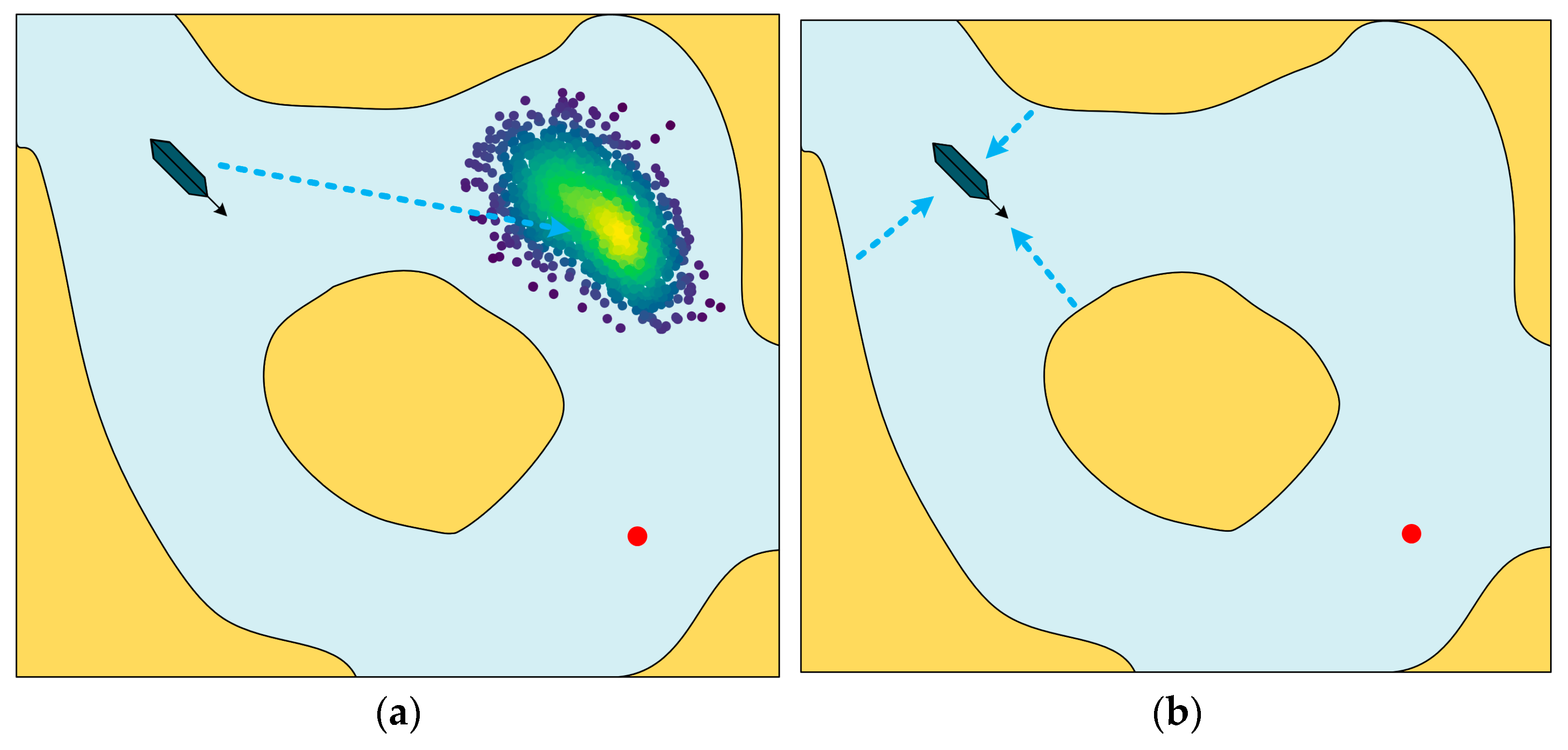
3.1. Artificial Potential Field Model

The artificial potential field model is a path planning method based on a virtual force field, which is inspired by the concept of the electric potential field or magnetic field in physics [23]. Its core idea is to guide the object to move safely and efficiently from the starting point to the end point by simulating the superposition of attraction and repulsion.

3.1.1. Gravitational Potential Field

The gravitational potential field is mainly related to the distance between the object and the target point. The greater the distance, the greater the potential energy value of the object, and vice versa. The calculation process of the gravitational potential field is shown in Equation (1):

$${\mathrm{U}}_{att}\left(\mathrm{q}\right)={\displaystyle \frac{1}{2}}\eta {\rho }^2\left(\mathrm{q},{\mathrm{q}}_{\mathrm{g}}\right)$$

(1)

where η is the gain coefficient of the proportional control term; ${\rho }^2\left(\mathrm{q},{\mathrm{q}}_{\mathrm{g}}\right)$ is a vector representing the Euclidean distance between the position q of the object and the position q_g of the target point.

Gravity ${\mathrm{F}}_{att}\left(\mathrm{q}\right)$ is the negative gradient of the gravitational field, representing the fastest changing direction of the gravitational potential field function 000. The calculation process of gravity is expressed as follows:

$${\mathrm{F}}_{att}\left(\mathrm{q}\right)=-\nabla {\mathrm{U}}_{att}\left(\mathrm{q}\right)=-\eta \rho \left(\mathrm{q},{\mathrm{q}}_{\mathrm{g}}\right)$$

(2)

3.1.2. Repulsive Potential Field

The repulsive potential field ensures that the object stays away from the obstacle. When the object does not enter the influence range of the obstacle, the potential energy value received is zero. As the object enters the influence range of the obstacle, the greater the distance, the smaller the potential energy value the object receives, and vice versa. The calculation process of the repulsive potential field is shown in Equation (3).

$${\mathrm{U}}_{req}\left(\mathrm{q}\right)=\left\{\begin{array}{c}{\displaystyle \frac{1}{2}}\mathrm{k}{\left({\displaystyle \frac{1}{\mathrm{p}\left(\mathrm{q},{\mathrm{q}}_0\right)}}-{\displaystyle \frac{1}{{\mathrm{p}}_0}}\right)}^2,0\le \mathrm{p}\left(\mathrm{q},{\mathrm{q}}_0\right)\le {\mathrm{p}}_0\\ 0,\mathrm{p}\left(\mathrm{q},{\mathrm{q}}_0\right)\ge {\mathrm{p}}_0\end{array}\right.$$

(3)

Here, k is the proportional coefficient; $\mathrm{p}\left(\mathrm{q},{\mathrm{q}}_0\right)$ is a vector representing the influence of obstacles on the movement of objects; and ${\mathrm{p}}_0$ denotes a constant of the maximum influence range. The calculation principle of the repulsive force is shown as follows:

$${\mathrm{F}}_{req}\left(\mathrm{q}\right)=\left\{\begin{array}{c}\mathrm{k}\left({\displaystyle \frac{1}{\mathrm{p}\left(\mathrm{q},{\mathrm{q}}_0\right)}}-{\displaystyle \frac{1}{{\mathrm{p}}_0}}\right){\displaystyle \frac{1}{{\mathrm{p}}^2\left(\mathrm{q},{\mathrm{q}}_0\right)}},0\le \mathrm{p}\left(\mathrm{q},{\mathrm{q}}_0\right)\le {\mathrm{p}}_0\\ 0,\mathrm{p}\left(\mathrm{q},{\mathrm{q}}_0\right)\ge {\mathrm{p}}_0\end{array}\right.$$

(4)

3.1.3. Resultant Potential Field

For a moving object, it is mainly affected by the gravitational potential field and the repulsive potential field. The combined potential field is written as is shown in Equation (5).

$$\mathrm{U}\left(\mathrm{q}\right)={\mathrm{U}}_{att}\left(\mathrm{q}\right)+{\mathrm{U}}_{req}\left(\mathrm{q}\right)$$

(5)

The magnitude of the resultant force is shown in Equation (6).

$$\mathrm{F}\left(\mathrm{q}\right)=-\nabla \mathrm{U}\left(\mathrm{q}\right)={\mathrm{F}}_{att}\left(\mathrm{q}\right)+{\mathrm{F}}_{req}\left(\mathrm{q}\right)$$

(6)

3.2. Introduction of A* Algorithm

As a heuristic search algorithm, the A* algorithm (A-Star Algorithm) has been widely adopted to obtain the shortest path from the starting point to the end point in a graph structure or grid map [24]. It combines the completeness of the breadth-first search (BFS) with the efficiency of the greedy algorithm, prioritizing the expansion of the most promising nodes by dynamically evaluating the path cost. The evaluation function is the critical part of the path planning, as shown in Equation (7):

$$F(n)=G(n)+H(n)$$

(7)

where G(n) is the actual cost from the starting node to node n in the state space. In general, Euclidean distance is used as the standard, and the calculation principle is demonstrated in Equation (8). H(n) is the heuristic estimated cost function from node n to the end point. In general, Manhattan distance is used as the heuristic function, and the calculation principle is expressed as is shown in Equation (9):

$$G(n)=\sqrt{{(X_n-X_{Start})}^2+{(Y_n-Y_{Start})}^2}$$

(8)

$$H(n)=\sqrt{{(X_n-X_{Goal})}^2+{(Y_n-Y_{Goal})}^2}$$

(9)

where (X_n, Y_n) is the current point; (X_Start, Y_Start) is the starting point; and (X_Goal, Y_Goal) denotes the target point.

3.3. A* Algorithm Integrated with Artificial Potential Field Model (APF-A*)

The traditional A* algorithm reduces the total mileage by approaching obstacles when planning the path, which leads to the occurrence of many inflection points. It differs with the navigation characteristics of small coastal vessels [25]. In the present study, the artificial potential field model has been introduced to optimize the A* algorithm, thereby generating the path and achieving trajectory repairing for small coastal vessels. The implementation of the APF-A* algorithm is shown in Figure 1, followed by a comprehensive description in Section 3.3.1, Section 3.3.2, Section 3.3.3, Section 3.3.4 and Section 3.3.5.

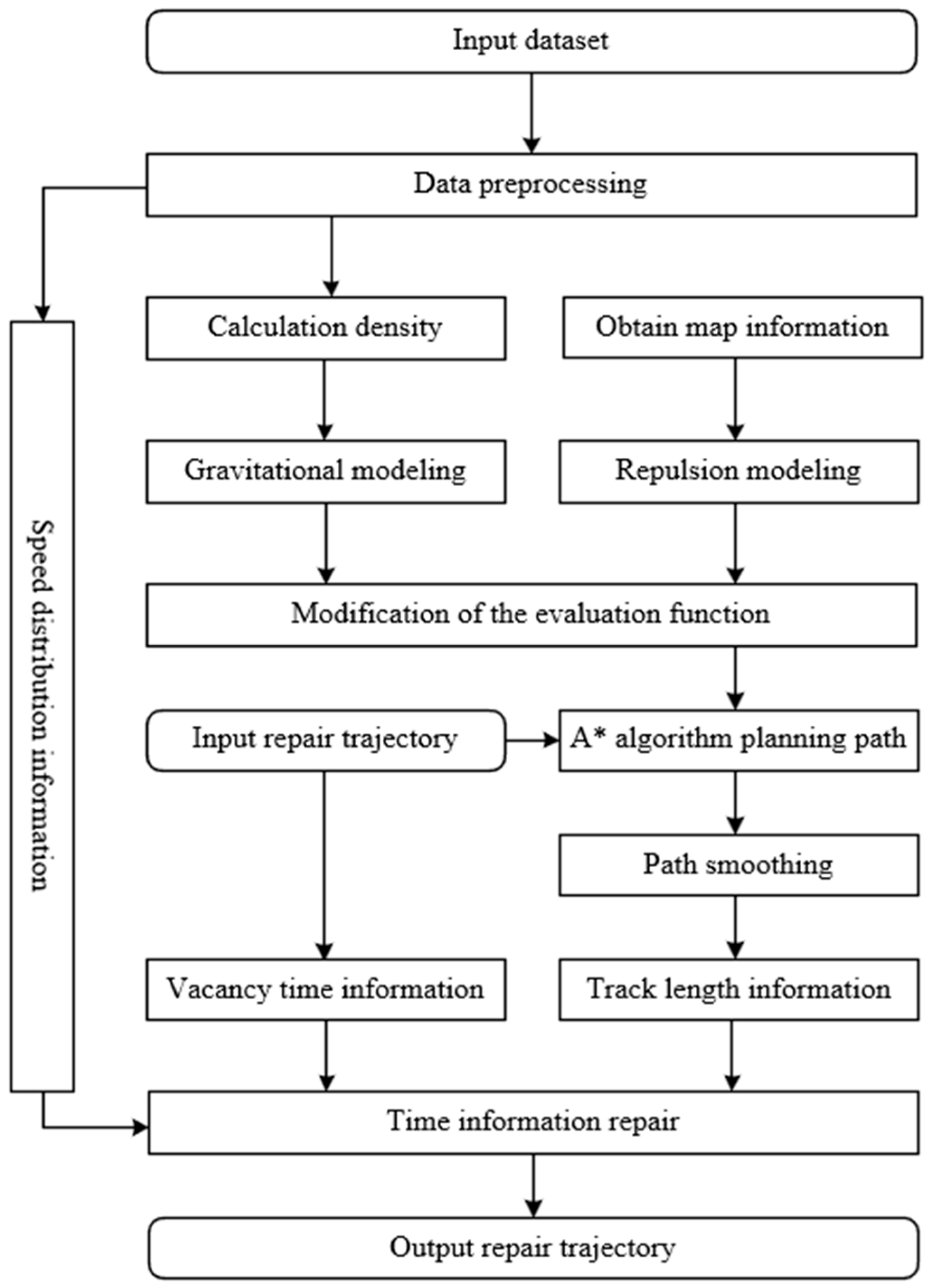
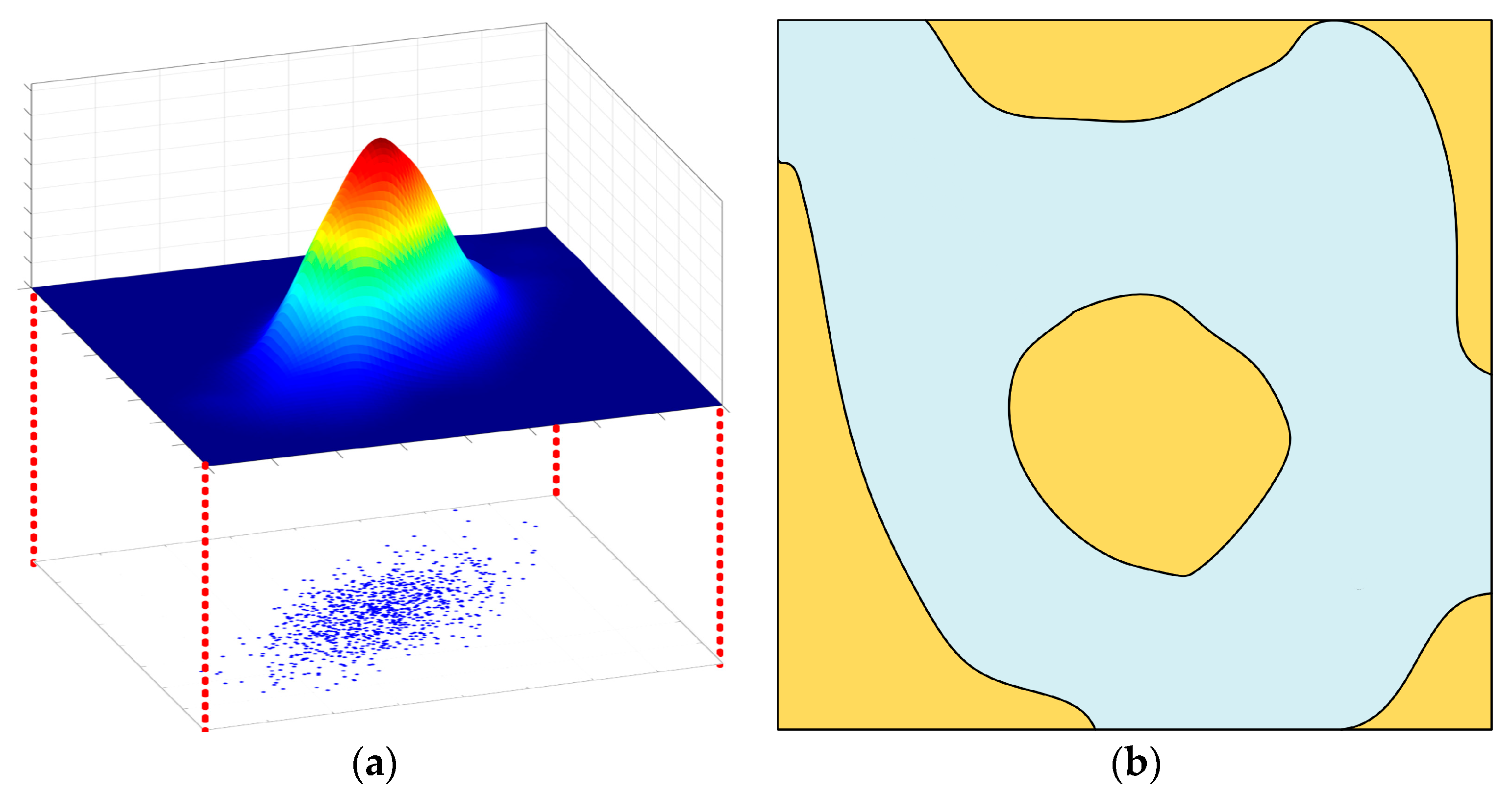
3.3.1. Data Preprocessing and Potential Field Construction

The core of ship trajectory repair is to restore the ship’s movement path. Therefore, anchoring data are generally excluded. The AIS data density field is then generated based on the ship’s movement point data. The density calculation is depicted in Equation (10). The density field generation process is shown in Figure 2a, where the raised part denotes areas with a higher density. The geographic constraint field is illustrated in Figure 2b, where light-blue and yellow areas represent navigable water and land, respectively.

$$Density(x,y)={\displaystyle \sum _{i=1}^N\exp \left(-\frac{{(x-x_i)}^2+{(y-y_i)}^2}{2{\sigma }^2}\right)}$$

(10)

3.3.2. Potential Field Function Reconstruction

In the artificial potential field algorithm, the gravitational potential field and gravitational magnitude of the potential field function are determined according to the position of the current point and the target point. The greater the distance, the greater the gravitational force. The algorithm proposed in this paper has been further optimized by setting the target of the gravitational field to the AIS data density field obtained in Section 3.3.1, and by setting the gravitational direction points to the direction of the density gradient increase. Meanwhile, the truncation function is adopted to avoid the excessive influence of the gravitational potential field on the path. The gravitational potential field size is calculated using Equation (11), and the truncation function is written as is shown in Equation (12).

$$U_{att}^{AIS}(x,y)=-k_{att}\cdot D{(x,y)}^{\gamma }+\lambda \cdot \Vert \nabla D(x,y)\Vert$$

(11)

$$U_{att}(x,y)=\left\{\begin{array}{cc}{U}_{att}^{AIS}(x,y)& U_{att}^{AIS}(x,y)>-{\displaystyle \frac{1}{\alpha }}\\ -{\displaystyle \frac{1}{\alpha }}& U_{att}^{AIS}(x,y)\le -{\displaystyle \frac{1}{\alpha }}\end{array}\right.$$

(12)

where k_att is the gravitational coefficient; D(x, y) is the trajectory point density value; $\nabla D(x,y)$ denotes the fastest changing direction of the density; γ is the nonlinear scaling factor; $\lambda$ represents the density gradient bootstrap weight; and α is the weight of the ensemble potential field in the evaluation function of the A* algorithm. Given the constant repulsive potential field, the ensemble potential field is represented by U(x, y) and its computational principle is demonstrated in Equation (13). The influence of the gravitational field is illustrated in Figure 3a. Differing from the artificial potential field algorithm, the closer the gravitational field is set in this paper, the stronger the gravitational force. The repulsive field is consistent with the artificial potential field method, and the direction is presented in Figure 3b.

$$U\left(x,y\right)=U_{att}\left(x,y\right)+U_{req}\left(x,y\right)$$

(13)

where U_att and U_req denote the gravitational and repulsive potential field, respectively.

3.3.3. Reconstruction of A* Algorithmic Evaluation Function

Generally, the traditional A* algorithm only considers the actual distance with the estimated cost. The algorithm for artificial potential field optimization is achieved by adding combined potential field, and the result is obtained as follows:

$$F(n)=G(n)+H(n)+\alpha U(x,y)$$

(14)

where α denotes the input parameter and U(x, y) is the ensemble potential field.

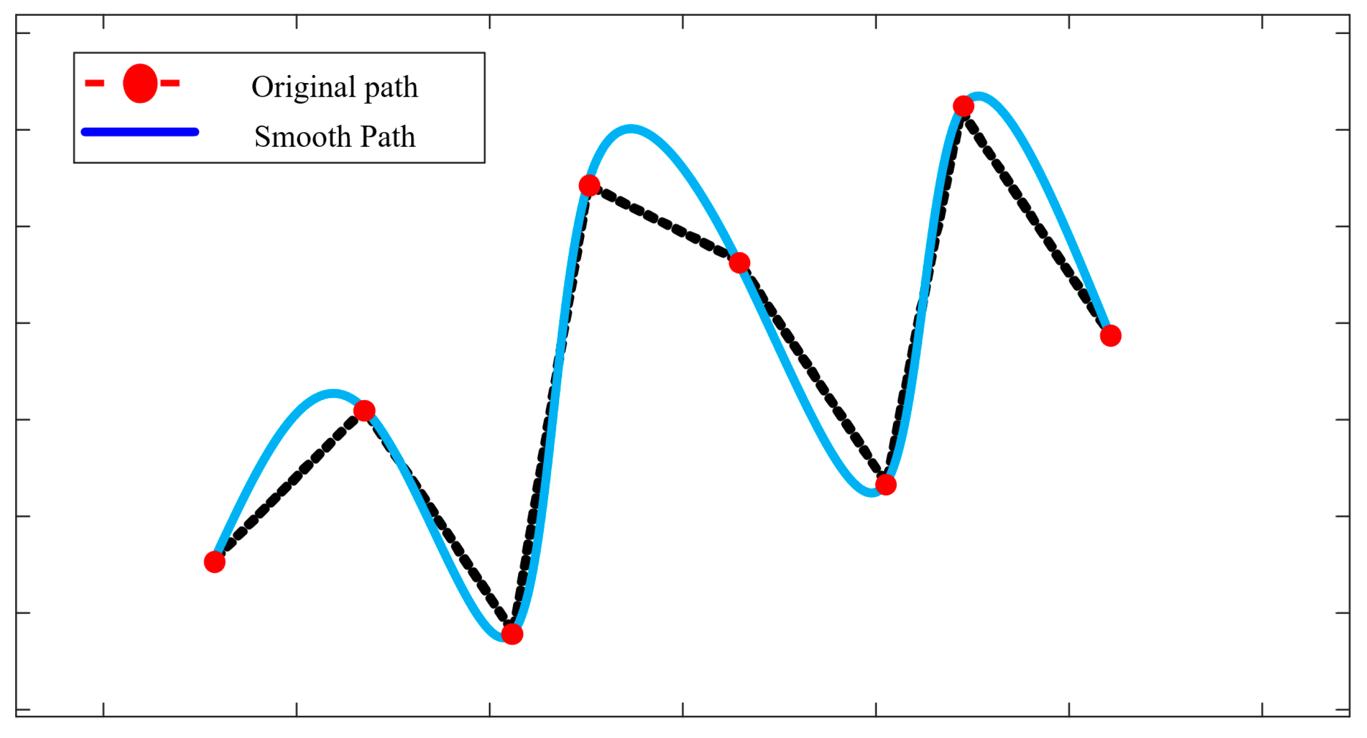
3.3.4. Path Smoothing

The paths obtained using the A* algorithm show obvious steering patterns, which differ greatly from the actual trajectories. As a result, the classical B spline curve [26] is introduced for path smoothing, as shown in Equation (15). The path shape can be further adjusted to conform with the ship motion trajectory (Figure 4).

$$\mathrm{p}(u)={\displaystyle \sum _{i=0}^n{q}_i{N}_{i,k(u)}}$$

(15)

where q_i denotes the control vertex coordinates and N_i,k(u) is the spline basis function. The Cox–deBoor model has been widely used, with the maximum number of times being denoted by k.

3.3.5. Temporal Information Repairing

Aimed at addressing the spatial–temporal coupling characteristics of AIS data, this study proposes a spatial–temporal collaborative repair mechanism based on the speed feature partition. As shown in Figure 5a–c, the method implementation contains the following three key stages: (1) Navigation feature partitioning is achieved based on the improved k-means++ algorithm [27]. The optimal number of clusters k is determined as 4 according to the contour coefficient method, and the parameters are input into the algorithm to obtain the four clusters shown in Figure 5a. (2) The navigation speed distribution is further characterized using a robust box-and-line plot using the graph-based method. The median sailing speed in each partition is selected as the typical feature value, and the horizontal coordinates in Figure 5b represent the different clusters. (3) The finalization of basin boundary optimization guided by expert knowledge is completed, as shown in Figure 5c, and the AIS time series of different regions are calculated based on the time information in the original data, the total sailing distance derived from the A* algorithm, and the typical feature values in the box-and-line diagrams.

4. Experimental Results

In this section, an experimental study was conducted to resolve the trajectory repair problem, and the experiment design contains the following key aspects: (1) a description of the experimental area; (2) a characterization of the dataset; (3) vessel speed feature extraction; and (4) trajectory repair based on the improved path planning algorithm. All numerical experiments were completed on a workstation configured with an Intel^® Core^TM i5-14600KF processor and an NVIDIA GeForce RTX 4060 graphics card. The workstation is equipped with 64 GB of RAM and a 4TB hard drive. The algorithm framework is constructed and implemented based on a Python 3.8 environment and scientific computing libraries (e.g., NumPy) to optimize matrix operations.

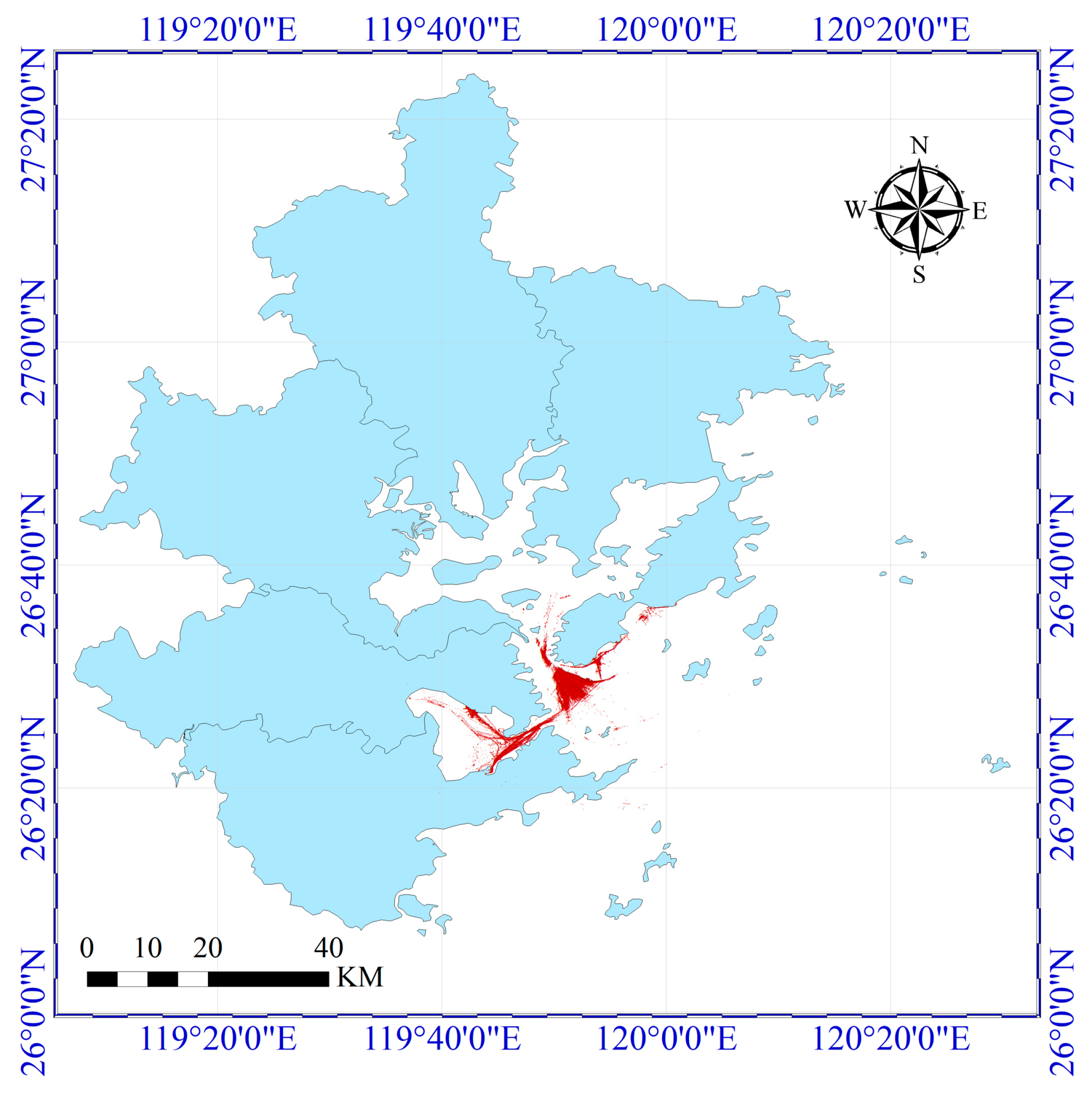
4.1. Description of the Study Area

Luoyuan Bay, which is located in Fujian Province, China, is a natural deep-water harbor on the coast of the East China Sea and is one of the six deep-water harbors in Fujian Province. It is surrounded by mountains on three sides, with a total area of about 230 square kilometers and a coastline of 129 km. The experimental data are derived from October to November 2023, ranging from 26.30 N to 26.65 N and from 119.6 E to 120.1 E. A total of 3538 ship trajectories and 5,728,509 data points are obtained. After data preprocessing, data of small coastal ships are extracted according to the ship type and size—specifically, ships with a length of less than 30 are firstly screened, and then the data are screened again according to the ship type with the AIS digital code, as shown in

Table 1. Ship types and corresponding digital codes.

Vessel Type	AIS Digital Coding
Fishing Boat	3
Self-use vessels	0, 1
Ferry	2
Agricultural transport ships	1, 19
Tourist sightseeing boats	7, 14
Law enforcement vessel	10
Engineering vessels	17, 20

. Finally, 988 ship trajectories with 96,596 data points are obtained, as shown in Figure 6, where the red color denotes the ship trajectory points.

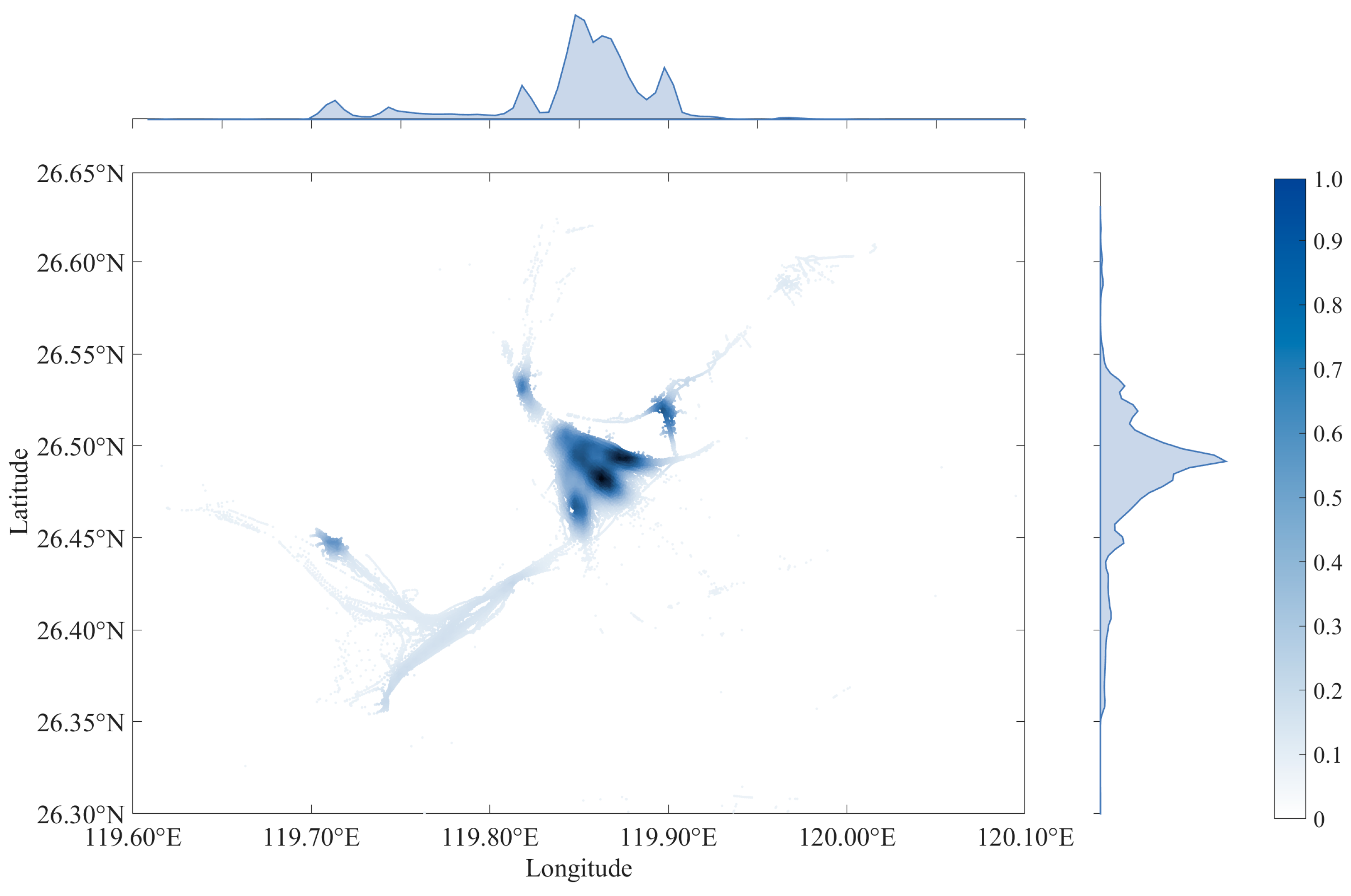
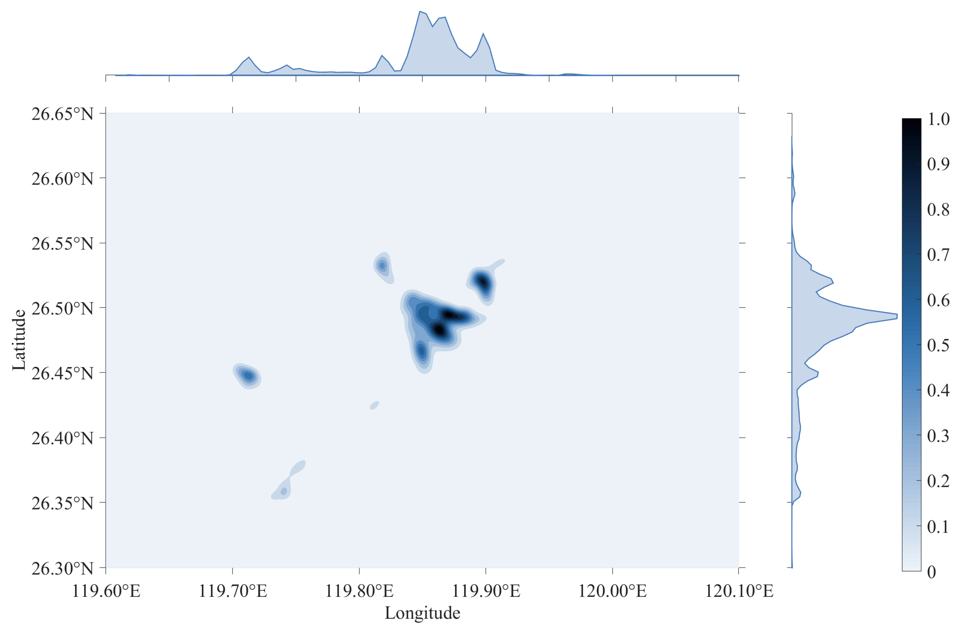
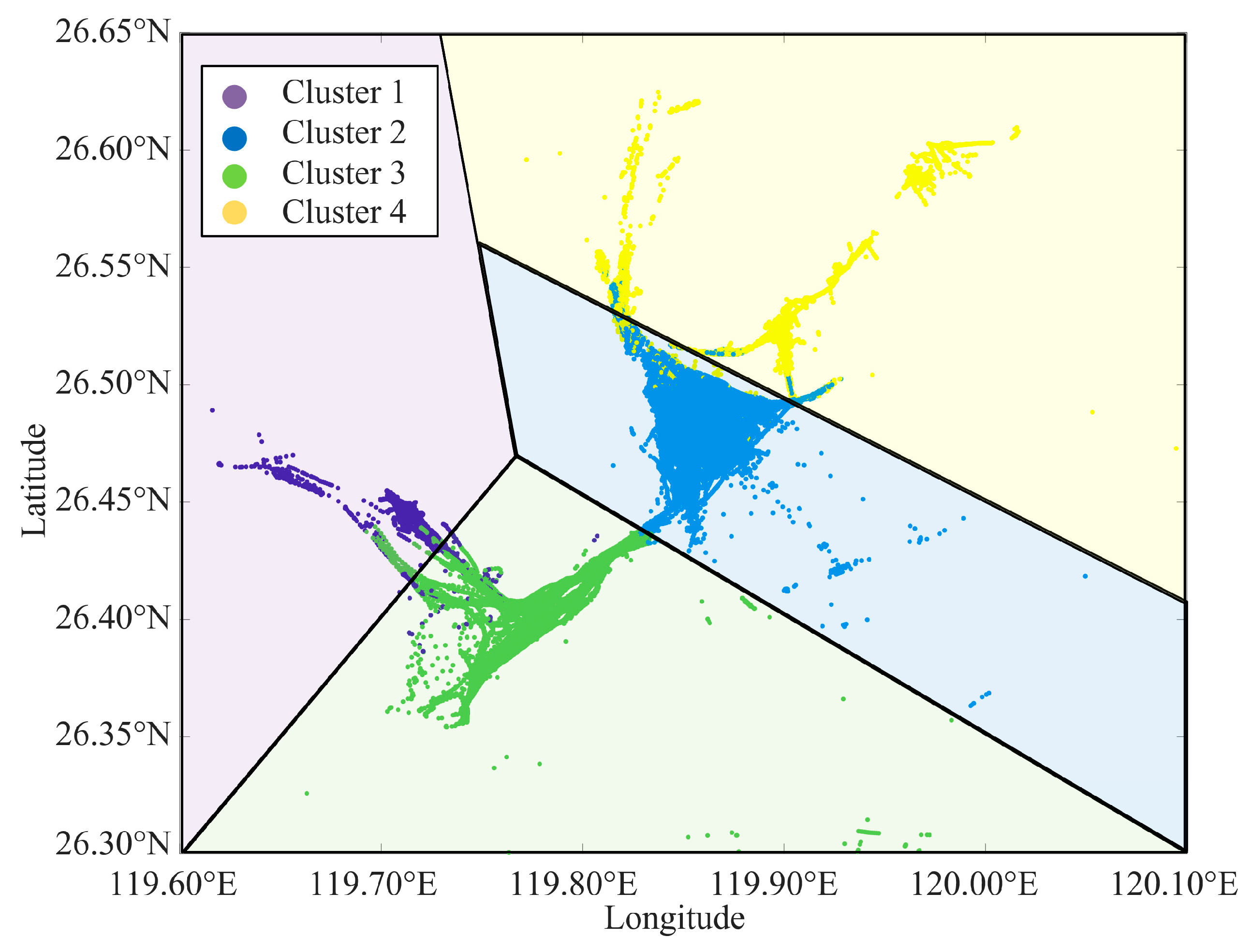
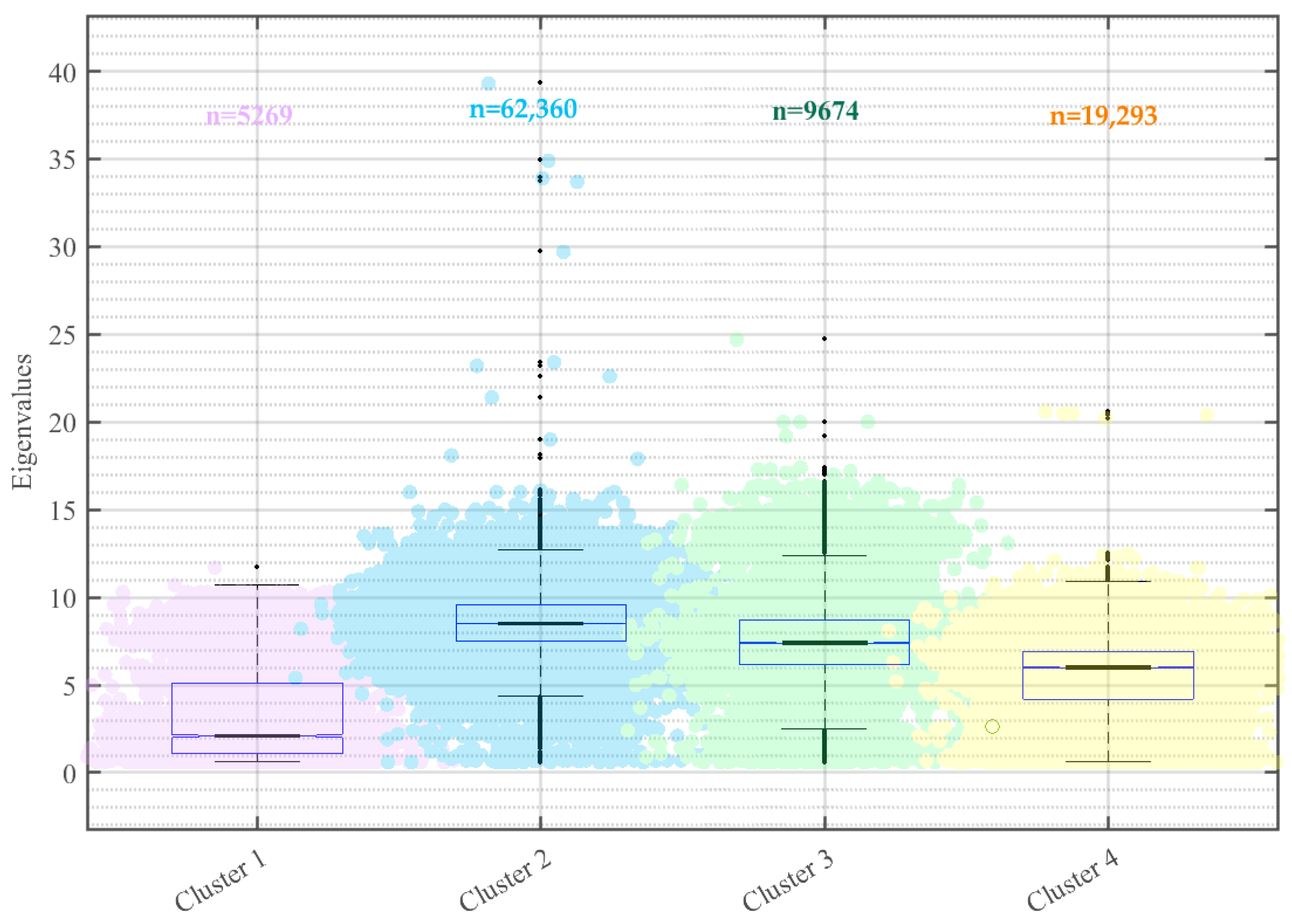
4.2. Density Calculation for Small Coastal Vessels

To achieve the goal of restoring the motion paths of small coastal vessels, a gravitational field model based on trajectory point density has been established. The latitude and longitude data are initially normalized, followed by kernel density estimation, with a grid size of 0.04 × 0.02 and a default bandwidth of 0.2975. As shown in Figure 7, the spatial distribution of vessel trajectory points exhibits a significant clustering pattern, with a particularly high point density in the outer waters of Luoyuan Bay. The horizontal and vertical axes represent the vessels’ longitude and latitude, respectively, providing an intuitive visualization of the spatial aggregation patterns of vessel activities. The density of data points at different locations is represented using different colors. The scatter density diagram reveals that the central region has a higher density compared to the surrounding areas. To enhance the visualization of spatial patterns, the scatter density diagram is converted into a contour map (Figure 8). By filtering out low-density noise, the gradient variations in the density of key navigation points are effectively highlighted. This optimized visualization significantly enhances the stratification and spatial structure of the data distribution, allowing for a clearer distinction between core high-density zones and peripheral low-density zones in vessel movement patterns. The contour map reveals distinctly concentrated areas of high trajectory density, which will be highly beneficial for the subsequent trajectory repairing process.

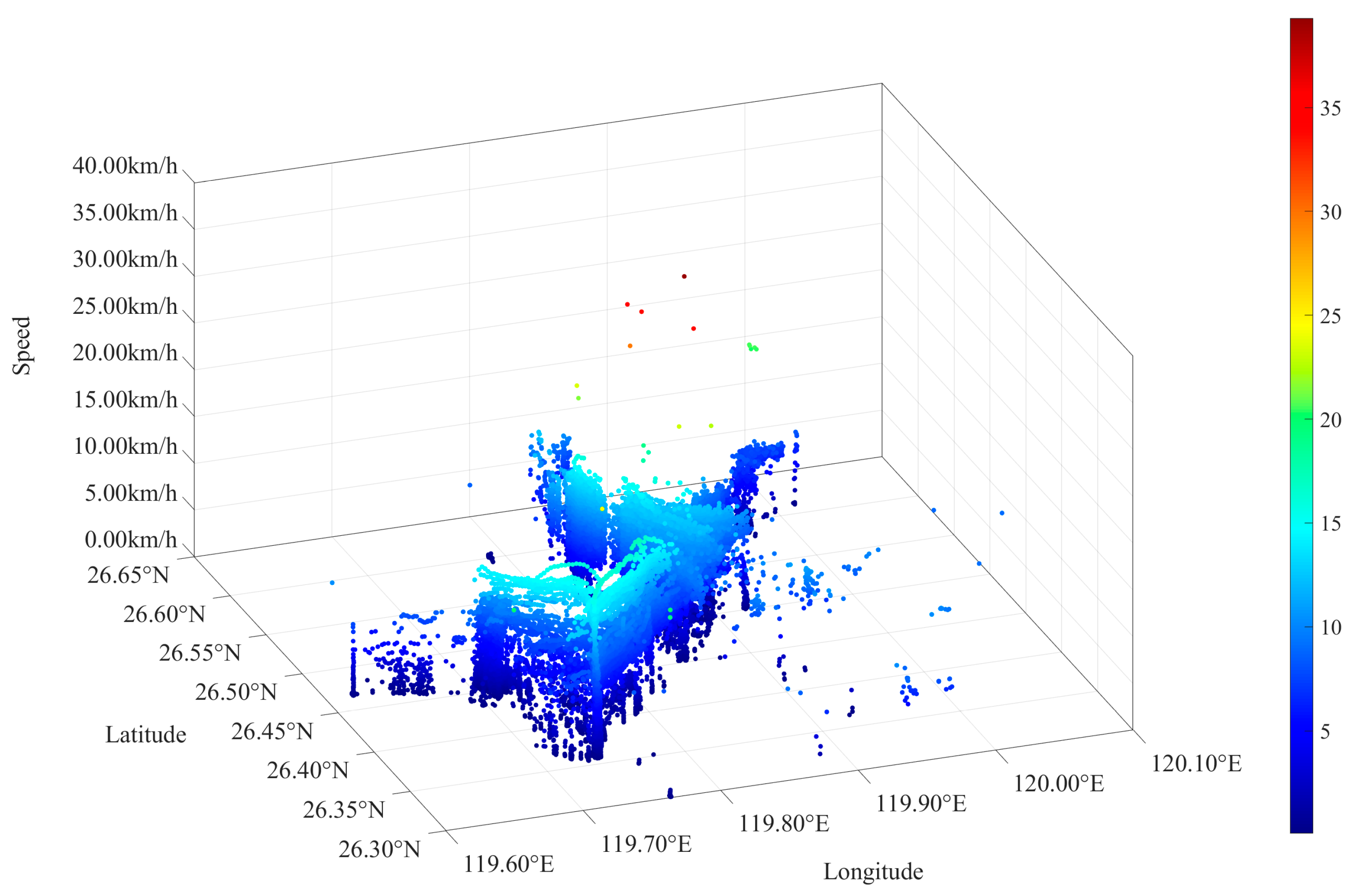
4.3. Feature Extraction of Vessel Speed

The vessel speed characteristics are critical to recovering trajectory time information. For small coastal vessels, sailing area and ship type are identified as key influencing factors of vessel speed. Therefore, the information of ship location (i.e., latitude and longitude), speed, and ship type are integrated to obtain a stepped distribution chart, as shown in Figure 9. The sensitivity of different information is balanced by normalization and is then clustered using the k-means++ algorithm. The number of clusters is optimized by using profile coefficients. The clustering and region division results are provided in Figure 10.

Meanwhile, boxplots were adopted to visualize the characteristics of vessel speeds across different regions (as shown in Figure 11). The horizontal axis represents the number of clusters, while the vertical axis indicates the speed features. The scatter point colors are consistent with the clustering results. Accordingly, the characteristic speeds for four navigational regions are identified as follows: the characteristic speed in the first type of navigation area is 2.1 km/h; it equals to 8.5 km/h, 7.5 km/h, and 6 km/h for the second, third, and fourth navigation areas. The vessel speed characteristics mainly represent the variation part rather than the absolute values. Therefore, the time information of the input trajectory points and the corresponding travel distance should be further processed.

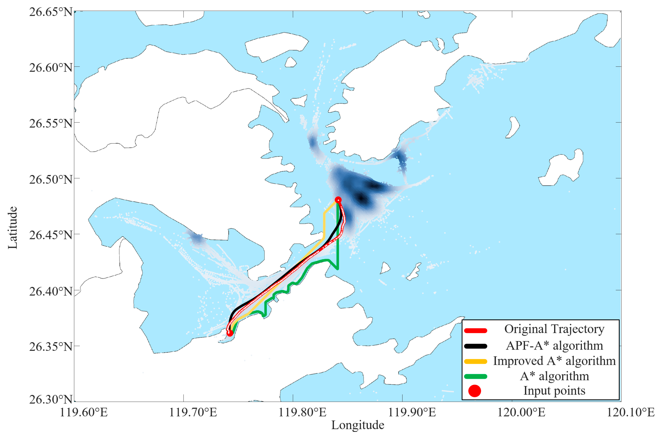
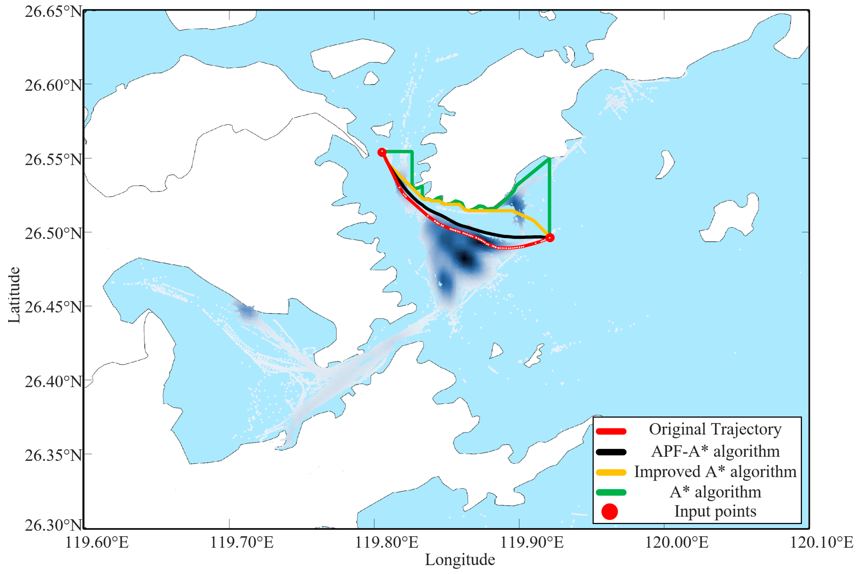
4.4. Comparative Study of Trajectory Repairing

To verify the effectiveness of the proposed trajectory repair algorithm, two small coastal vessels with representative navigational characteristics have been selected for comparative study. The first case involved trajectory data generated by the vessel with MMSI 336869665 between 11:43 and 13:44 on 19 October 2023. The second case corresponds to the vessel with MMSI 200008266, collected between 07:45 and 08:45 on 21 October 2023. In the present study, extreme input conditions were simulated; only the starting and ending trajectory points were retained as model inputs. The reconstruction of the entire missing segment was explored and evaluated. Two different path planning algorithms were introduced as baselines. The A* algorithm [28] is a classical path planning method that relies entirely on input data points and environmental constraints. It adopts the neighborhood search rule. Meanwhile, the Manhattan distance and the actual travel distance are incorporated as the heuristic and cost function, respectively. An improved A* algorithm, which was proposed by Kaklis et al. [29], enhances the A* method by incorporating historical AIS data and utilizing a convex hull algorithm to define navigable regions. Finally, the proposed APF-A* algorithm was evaluated. The experimental results are demonstrated in Figure 12 and Figure 13.

Case 1, as shown in Figure 12, provides a typical navigation scenario involving a vessel entering and exiting Luoyuan Bay. The results indicate that the trajectory generated using the traditional A* algorithm (green line) exhibits a significant spatial deviation from the reference trajectory, with the path closely hugging the shoreline. This topological pattern is inconsistent with actual vessel maneuvering characteristics and raises safety concerns. The improved A* algorithm (yellow line) achieves local conformity to the reference trajectory but still shows an unsafe proximity to the shore in certain segments, reflecting the limitations of relying solely on navigational region constraints. In contrast, the APF-A* algorithm (black line) demonstrates superior global topological alignment. Its heading angle sequence closely matches that of the reference trajectory, and its spatial configuration yields the highest structural similarity. The results of Case 2, presented in Figure 13, show a consistent trend with those of Case 1. Both the traditional A* and improved A* algorithms suffer from systematic near-shore deviations, failing to meet the 0.5 nautical mile safety margin recommended by the International Maritime Organization (IMO). The APF-A* algorithm, through repulsive force modeling in the potential field, effectively maintains a safe navigational envelope. However, its geometric fidelity to the original trajectory slightly decreases compared to that of Case 1, primarily due to the convergent variations induced by the gravitational field magnitude constraints. With the aid of the artificial potential field optimization framework, the APF-A* algorithm would produce more accurate geometric characteristics for real-world navigation paths.

4.5. Discussion

In the quantitative evaluation of vessel trajectory reconstruction performance, this study adopts a three-dimensional assessment framework to facilitate objective comparison. Specifically, Hausdorff Distance (HD) [30], Dynamic Time Warping (DTW) [31], and an Improved Distance Loss (DL) metric are selected as the core evaluation indicators. HD is employed to measure the spatial deviation between the reconstructed trajectory and the ground truth trajectory. DTW captures the shape similarity between trajectory sequences by leveraging its nonlinear time alignment mechanism. DL quantifies the geometric integrity of the reconstructed path by computing the absolute difference in total path length. The mathematical definitions and calculation formulas of these metrics are provided in Equations (16)–(18). This multi-perspective evaluation system enables a comprehensive characterization of the trajectory repairing quality in terms of spatial distribution, temporal dynamics, and geometric consistency.

For two discrete trajectories T₁ = {a₁, …, a_m} and T₂ = {b₁, …, b_n}, the Hausdorff Distance is defined as follows:

$$\left.H(T_1,T_2)=\max \left\{\underset{a\in T_1}{\max }\underset{b\in T_2}{\min }d(a,b),\underset{b\in T_2}{\max }\underset{a\in T_1}{\min }d(a,b)\right.\right\}$$

(16)

Dynamic Time Warping is defined as follows:

$$\mathrm{DTW}(T_1,T_2)=\underset{\pi \in \mathsf{\Pi }}{\min }\sum _{(i,j)\in \pi }\parallel a_i-b_j{\parallel }_2$$

(17)

where Π denotes the combination satisfying the shortest move matrix.

Distance Loss is defined as follows:

$$\mathrm{Loss}(T_1,T_2)=\left|\sum _{i=2}^m\parallel a_i-a_{i-1}{\parallel }_2-\sum _{j=2}^n\parallel b_j-b_{j-1}{\parallel }_2\right|$$

(18)

where ${\displaystyle \sum _{i=2}^m}\parallel a_i-a_{i-1}{\parallel }_2$ denotes the cumulative value of the trajectory T₁; ${\displaystyle \sum _{j=2}^n}\parallel b_j-b_{j-1}{\parallel }_2$ represents the cumulative value of the trajectory T₂.

The calculation results of all performance indicators are shown in

Table 2. Calculation results of various performance indicators.

Experiments	Algorithms	HD	DTW	DL
Case 1	APF-A*	0.0033	2.5468	0.1035
	Improve A*	0.0180	12.3136	0.1192
	A*	0.0229	35.7881	0.2230
Case 2	APF-A*	0.0352	10.9357	0.1154
	Improve A*	0.0947	129.5199	0.1098
	A*	0.1873	320.3494	0.1930

, where the bold font represents the optimal performance values.

With regard to two-dimensional trajectory data, the Hausdorff Distance (HD) represents the maximum spatial deviation between the repaired and reference trajectories. Dynamic Time Warping (DTW) distance reflects the similarity in trajectory shape, and Distance Loss (DL) measures the degree of variation in the trajectory length. As shown in Table 1, the evaluation results are generally consistent with the visual analysis shown in Figure 12 and Figure 13. The APF-A* algorithm consistently outperforms the other methods across multiple metrics. In Case 1, the DTW values are relatively low overall (ranging from 2.5468 to 35.7881). Notably, the DTW score of the APF-A* algorithm (2.5468) accounts for only 7.12% of the conventional A* algorithm, indicating that the path smoothing effect in complex turning regions effectively mitigates trajectory distortion. From the perspective of spatial accuracy, the HD of the APF-A* algorithm (0.0033) is reduced by 81.67% and 85.59% compared to the improved A* and traditional A* algorithms, respectively. This improvement stems from the obstacle-avoidance optimization embedded in the artificial potential field (APF) framework. In terms of DL, although the APF-A* algorithm (0.1035) differs from the improved A* (0.1192) by approximately 13.4%, it achieves a 53.58% improvement over the conventional A*, highlighting the effectiveness of the proposed method in controlling trajectory length. The expanded scenario in Case 2 further validates the distinctions among different algorithms. The APF-A* algorithm continues to lead with an HD of 0.0352 and a DTW of 10.9357, representing improvements of 81.20% and 96.59% over the A* algorithm, respectively. Particularly, the DTW metric reveals an order-of-magnitude difference, with the shape fidelity of the APF-A* trajectory reaching 11.84 times that of the improved A* algorithm. This can be attributed to the potential field mechanism introduced in APF-A*, which enhances conformity to realistic vessel motion patterns. Interestingly, the improved A* algorithm achieves a slightly lower DL value (0.1098) than the APF-A* (0.1154)—a 0.56% margin—possibly due to a coincidental similarity in total trajectory length when the curvature directions counterbalance each other. To summarize, the APF-A* algorithm presents significant advantages in HD and DL metrics, outperforming the traditional A* algorithm by an average of 85.38% in HD (from 0.0196 in Case 1 to 0.1521 in Case 2) and achieving order-of-magnitude improvements in DTW (from 33.2413 in Case 1 to 309.4137 in Case 2). The comparative study validates the strong adaptability of the APF-A* algorithm under complex navigational scenarios.

In conclusion, the proposed APF-A* algorithm exhibits clear advantages in minimizing trajectory deviation (HD) and path length variation (DL). Most notably, it achieves a superior shape similarity (DTW), owing to the integration of repulsive potential fields, which align with the maritime navigational habits of avoiding proximity to shorelines.

5. Conclusions

The present study addresses the issue of AIS data loss for small coastal vessels operating in nearshore waters by proposing a trajectory repairing model based on the artificial potential field-enhanced A* algorithm (APF-A*). By integrating kernel density estimation with potential field theory, the model constructs an attractive potential field derived from historical trajectories and a repulsive potential field considering topographic constraints. Additionally, it incorporates speed distribution characteristics and spatiotemporal constraints to achieve the joint optimization of both the spatial structure and temporal attributes of the repaired trajectories. An experimental study was conducted in Luoyuan Bay, Fujian Province, and the results demonstrate that the APF-A* algorithm significantly outperforms conventional approaches. Specifically, it reduces the Hausdorff Distance (HD) by an average of 85.38% compared to the traditional A* algorithm, as well as achieving order-of-magnitude improvements in the Dynamic Time Warping (DTW) with reductions of 91.56% in Case 1 and 96.59% in Case 2. The proposed model innovatively integrates historical AIS data into the path reconstruction process, enabling the effective restoration of both speed and timestamp information.

These findings fill the research gap in the field of trajectory repairing for small coastal vessels and provide a promising tool for enhancing maritime safety administration. However, certain limitations still remain. The computational complexity increases as historical data are adopted to construct the attractive potential field. The current framework does not fully account for dynamic speed variations throughout the entire voyage, overlooking the impact of speed changes caused by weather, currents, and vessel-specific factors. Meanwhile, the present study focuses on the small coastal vessels in Luoyuan Bay. Future work will explore trajectory clustering based on origin–destination pairs to identify relevant historical trajectory datasets. The accuracy of vessel speed recovery could be enhanced by incorporating navigation environment conditions and vessel characteristics. The robustness of the proposed algorithm can be validated on widely collected datasets, thus providing guidance for accident prevention in coastal waters.

References

1. Shipton, M.; Obradović, J.; Mišković, N.; Diamant, R. Underwater Radiated Noise Characteristics of Small Vessels—An Analysis of the HearMyShip Database. Mar. Pollut. Bull. 2025, 216, 117903. [Google Scholar] [CrossRef] [PubMed]
2. Smith, T.A.; Grech La Rosa, A.; Wood, B. Underwater Radiated Noise from Small Craft in Shallow Water: Effects of Speed and Running Attitude. Ocean Eng. 2024, 306, 118040. [Google Scholar] [CrossRef]
3. Alves, C.L.; Garcia, O.D.; Kramer, R.A. Fisher Perceptions of Belize’s Managed Access Program Reveal Overall Support but Need for Improved Enforcement. Mar. Policy 2022, 143, 105192. [Google Scholar] [CrossRef]
4. Zhang, H.; Li, K. Assessment of Fishing Vessel Vulnerability to Pure Loss of Stability Using a Self-Developed Program. J. Mar. Sci. Eng. 2024, 12, 527. [Google Scholar] [CrossRef]
5. Xiao, G.; Yang, D.; Xu, L.; Li, J.; Jiang, Z. The Application of Artificial Intelligence Technology in Shipping: A Bibliometric Review. J. Mar. Sci. Eng. 2024, 12, 624. [Google Scholar] [CrossRef]
6. Ahn, S.; Pomeroy, R. Evaluating the Economic Impact of Distant Water Fleet Activities on Small-Scale Fishers in the South China Sea. Mar. Policy 2024, 168, 106324. [Google Scholar] [CrossRef]
7. Zhang, L.; Zhu, Y.; Valdez Banda, O.A.; Du, L.; Gan, L.; Li, X. Navigational Risk Assessment of Inland Waters Based on Bi-Directional PSO-LSTM Algorithm and Ship Maneuvering Characteristics. Ocean Eng. 2024, 310, 118628. [Google Scholar] [CrossRef]
8. Wen, Z.; Zhang, X.; Liu, S.; Zheng, Z.; Zhang, T.; Liao, Z.; Xia, X.; Li, Y. Multi-Level Localization Trajectory Alignment and Repairing in Complex Environment. Int. J. Appl. Earth Obs. Geoinf. 2024, 131, 103945. [Google Scholar] [CrossRef]
9. Zaman, B.; Marijan, D.; Kholodna, T. Interpolation-Based Inference of Vessel Trajectory Waypoints from Sparse AIS Data in Maritime. J. Mar. Sci. Eng. 2023, 11, 615. [Google Scholar] [CrossRef]
10. Du, H.; Xiao, Y.; Duan, L.; Gao, S. An Algorithm for Vessel’s Missing Trajectory Restoration Based on Polynomial Interpolation. In Proceedings of the 2017 4th International Conference on Transportation Information and Safety (ICTIS), Banff, AB, Canada, 8–10 August 2017; IEEE: New York, NY, USA, 2017; pp. 825–830. [Google Scholar] [CrossRef]
11. Zhang, C.; Liu, S.; Guo, M.; Liu, Y. A Novel Ship Trajectory Clustering Analysis and Anomaly Detection Method Based on AIS Data. Ocean Eng. 2023, 288, 116082. [Google Scholar] [CrossRef]
12. Guo, S.; Mou, J.; Chen, L.; Chen, P. Improved Kinematic Interpolation for AIS Trajectory Reconstruction. Ocean Eng. 2021, 234, 109256. [Google Scholar] [CrossRef]
13. Ye, L.; Chen, X.; Liu, H.; Zhang, R.; Li, J.; Lu, C.; Zhao, Y. A Study of Multi-Step Sparse Vessel Trajectory Restoration Based on Feature Correlation. Appl. Sci. 2024, 14, 4057. [Google Scholar] [CrossRef]
14. Kim, T.; Park, T.-H. Extended Kalman Filter (EKF) Design for Vehicle Position Tracking Using Reliability Function of Radar and Lidar. Sensors 2020, 20, 4126. [Google Scholar] [CrossRef] [PubMed]
15. Zhao, P.; Zhang, A.; Zhang, C.; Li, J.; Zhao, Q.; Rao, W. ATR: Automatic Trajectory Repairing With Movement Tendencies. IEEE Access 2020, 8, 4122–4132. [Google Scholar] [CrossRef]
16. Luo, Q.; Xu, Z.; Zhang, Y.; Igene, M.; Bataineh, T.; Soltanirad, M.; Jimee, K.; Liu, H. Vehicle Trajectory Repair Under Full Occlusion and Limited Datapoints with Roadside LiDAR. Sensors 2025, 25, 1114. [Google Scholar] [CrossRef]
17. Gao, D.; Zhu, Y.; Zhang, J.; He, Y.; Yan, K.; Yan, B. A Novel MP-LSTM Method for Ship Trajectory Prediction Based on AIS Data. Ocean Eng. 2021, 228, 108956. [Google Scholar] [CrossRef]
18. Xue, H. Fractional-Order Gradient Descent with Momentum for RBF Neural Network-Based AIS Trajectory Restoration. Soft Comput. 2021, 25, 869–882. [Google Scholar] [CrossRef]
19. Zhang, W.; Jiang, W.; Liu, Q.; Wang, W. AIS Data Repair Model Based on Generative Adversarial Network. Reliab. Eng. Syst. Saf. 2023, 240, 109572. [Google Scholar] [CrossRef]
20. Wu, Y.; Liu, D.; Tan, Y.; Duan, M.; Luo, L.; Wang, W.; Chen, X. LFPR: A Lazy Fast Predictive Repair Strategy for Mobile Distributed Erasure Coded Cluster. IEEE Internet Things J. 2023, 10, 704–719. [Google Scholar] [CrossRef]
21. Xia, Z.; Wang, W.; Guo, Z.; Peng, Y.; Tian, Q.; Xu, X. Navigation Mode Extraction and Trajectory Repair of Complex Waters in Multi-Harbor Port: An Optimal Semi-Supervised Clustering Method. Ocean Eng. 2024, 313, 119439. [Google Scholar] [CrossRef]
22. Liang, M.; Su, J.; Liu, R.W.; Lam, J.S.L. AISClean: AIS Data-Driven Vessel Trajectory Reconstruction under Uncertain Conditions. Ocean Eng. 2024, 306, 117987. [Google Scholar] [CrossRef]
23. Suo, Y.; Chen, X.; Yue, J.; Yang, S.; Claramunt, C. An Improved Artificial Potential Field Method for Ship Path Planning Based on Artificial Potential Field—Mined Customary Navigation Routes. J. Mar. Sci. Eng. 2024, 12, 731. [Google Scholar] [CrossRef]
24. He, Z.; Liu, C.; Chu, X.; Negenborn, R.R.; Wu, Q. Dynamic Anti-Collision A-Star Algorithm for Multi-Ship Encounter Situations. Appl. Ocean Res. 2022, 118, 102995. [Google Scholar] [CrossRef]
25. Huang, Y.; Zhao, S.; Zhao, S. Ship Trajectory Planning and Optimization via Ensemble Hybrid A* and Multi-Target Point Artificial Potential Field Model. J. Mar. Sci. Eng. 2024, 12, 1372. [Google Scholar] [CrossRef]
26. Ni, Q.; Xie, C. Stretch-Energy-Minimizing B-Spline Interpolation Curves and Their Applications. Mathematics 2023, 11, 4534. [Google Scholar] [CrossRef]
27. Ran, X.; Suyaroj, N.; Tepsan, W.; Ma, J.; Zhou, X.; Deng, W. A Hybrid Genetic-Fuzzy Ant Colony Optimization Algorithm for Automatic K-Means Clustering in Urban Global Positioning System. Eng. Appl. Artif. Intell. 2024, 137, 109237. [Google Scholar] [CrossRef]
28. Chatzisavvas, A.; Dossis, M.; Dasygenis, M. Optimizing Mobile Robot Navigation Based on A-Star Algorithm for Obstacle Avoidance in Smart Agriculture. Electronics 2024, 13, 2057. [Google Scholar] [CrossRef]
29. Kaklis, D.; Kontopoulos, I.; Varlamis, I.; Emiris, I.Z.; Varelas, T. Trajectory Mining and Routing: A Cross-Sectoral Approach. J. Mar. Sci. Eng. 2024, 12, 157. [Google Scholar] [CrossRef]
30. Chang, S.-C.; Jeng, J.-T. Interval Generalized Improved Fuzzy Partitions Fuzzy C-Means Under Hausdorff Distance Clustering Algorithm. Int. J. Fuzzy Syst. 2025, 27, 834–852. [Google Scholar] [CrossRef]
31. Herrmann, M.; Webb, G.I. Amercing: An Intuitive and Effective Constraint for Dynamic Time Warping. Pattern Recognit. 2023, 137, 109333. [Google Scholar] [CrossRef]
Figure 1. Implementation flowchart of the APF-A* algorithm.
Jmse 13 01200 g001
Figure 2. Schematic diagram of potential field setup. (a) Gravity potential field setting principle; (b) repulsion potential field setting principle.
Jmse 13 01200 g002
Figure 3. Potential field diagram. (a) Gravitational potential field; (b) repulsive potential field.
Jmse 13 01200 g003
Figure 4. Schematic diagram of path smoothing.
Jmse 13 01200 g004
Figure 5. Spatial–temporal collaborative repairing mechanism. (a) Navigational feature partitioning using the k-means++ algorithm. (b) Box-and-line diagram of sailing speed distribution. (c) Expert knowledge-guided watershed boundary optimization.
Jmse 13 01200 g005
Figure 6. The location of Luoyuan Bay, Fujian Province, and small coastal vessel data distribution.
Jmse 13 01200 g006
Figure 7. Scatter density distribution of small coastal vessels.
Jmse 13 01200 g007
Figure 8. Contour map of spatial distribution patterns for small coastal vessels.
Jmse 13 01200 g008
Figure 9. Longitude and latitude speed distribution charts.
Jmse 13 01200 g009
Figure 10. Results of K-means++ clustering and region delineation.
Jmse 13 01200 g010
Figure 11. Voyage speed distribution results for different clusters.
Jmse 13 01200 g011
Figure 12. Experiment results for Case 1.
Jmse 13 01200 g012
Figure 13. Experiment results for Case 2.
Jmse 13 01200 g013