Enhancing Fault Detection in AUV-Integrated Navigation Systems: Analytical Models and Deep Learning Methods

Abstract

In complex underwater environments, the stability of navigation for autonomous underwater vehicles (AUVs) is critical for mission success. To enhance the reliability of the AUV-integrated navigation system, fault detection technology was investigated. Initially, the causes and classifications of faults within the integrated navigation system were analyzed in detail, and these faults were categorized as either abrupt or gradual, based on variations in sensor output characteristics under fault conditions. To overcome the limitations of the residual chi-square method in detecting gradual faults, a cumulative residual detection approach with error coefficient amplification was proposed. The algorithm enhances gradual fault detection by using eigenvalue analysis and constructing fault-frequency-based error amplification coefficients with non-parametric techniques. Furthermore, to improve the detection of gradual faults, artificial intelligence-based fault detection methods were also explored. Specifically, the particle swarm optimization (PSO) algorithm was employed to optimize the hyperparameters of a long short-term memory (LSTM) neural network, leading to the development of a PSO-LSTM fault detection model. In this model, the fault detection function was formulated by comparing the predictions generated by the PSO-LSTM model with those derived from the Kalman filter. The experimental results demonstrated that the fault detection function formulated by PSO-LSTM exhibited enhanced sensitivity to gradual faults and enabled the timely isolation of faulty sensors. In unfamiliar marine regions, the PSO-LSTM method demonstrates greater stability and avoids the need to recalibrate detection thresholds for each sea area—an important advantage for AUV autonomous navigation in complex environments.

1. Introduction

As the operating range and mission duration of autonomous underwater vehicles (AUVs) continue to expand, the dynamic underwater environment may compromise the stability of output values from various subsystems in the AUV’s integrated navigation system, consequently reducing the accuracy of information fusion. Therefore, the implementation of efficient fault detection techniques for AUV navigation and positioning systems is considered one of the critical factors in ensuring the success of their missions.

Fault detection in AUV-integrated navigation systems is associated with numerous challenges [1,2]. Key challenges include the underwater environment’s complexity, real-time constraints, sensor failures, energy limitations, modeling uncertainties, low system adaptability, and a lack of historical data. Addressing these challenges requires fault detection algorithms that can identify various sensor faults accurately, operate in real time, and use minimal energy in unpredictable underwater conditions. Fault detection functions help identify faults in the navigation system and support timely corrective actions. Currently, three commonly used fault detection methods are as follows:

Analytical model-driven fault detection techniques are employed to extract fault information from a system under the assumption that its mathematical model is known. This technique may be categorized into distinct types, including state observation methods, parameter estimation methods, and equivalent space methods [3,4]. The state estimation method is implemented within the framework of a Kalman filter system and utilizes residual or state observers for fault detection [4]. Liu et al. utilized t-test and decoupling matrix methods to identify faults in gyroscopes and accelerometers [5,6]. Zhu et al. employed the chi-square test to exclude abnormal values from external sensors in integrated navigation systems [7]. Chu et al. developed a sliding mode observer, which was applied to fault reconstruction in underwater thrusters [8]. The parameter estimation method is primarily used to identify faults by analyzing the statistical characteristics of changes in system inputs and model output parameters. Mu et al. utilized variational Bayesian theory to estimate the measurement error covariance of t the Doppler velocity log (DVL) within an integrated INS-DVL navigation system and employed Euclidean distance to identify abnormal measurements [9]. Jin et al. proposed a tightly coupled approach employing an adaptive Kalman filter to dynamically estimate observation noise [10]. Yao et al. utilized statistical similarity measures to quantify the similarity between two random vectors derived from the DVL, developing a cost function to retain measurement information [11]. The equivalent space method detects faults by categorizing abnormal data. However, fault detection in real-time navigation systems requires continuous monitoring, but the equivalent space method depends on offline data from the integrated navigation system, rendering it unsuitable for real-time applications and thereby limiting its practical utility. Analytical model-based fault detection algorithms are commonly used in integrated navigation systems, although these methods depend on the accuracy of model parameters, and their detection thresholds are typically determined through engineering heuristics.

Signal processing-based fault detection algorithms are used to detect faults through the analysis of statistical characteristics of signals. In integrated navigation systems, the feature extraction process for time domain signals is centered on values such as extrema, root mean square values, and mean errors. Abid et al. developed an enhanced sequential SPRT fault detection algorithm aimed at addressing potential sensor faults in integrated navigation systems. Utilizing a sliding window to reset values to zero, the algorithm addresses the detection delay issue in conventional SPRT methods and demonstrates effectiveness in detecting both gradual and sudden faults [12]. Wang Gang et al. introduced a multi-view feature selection scheme incorporating information complementarity and consensus, which efficiently identifies relevant features for fault diagnosis [13].

With the development of artificial intelligence (AI) technologies, knowledge-based fault detection methods have gained significant attention. These methods primarily rely on convolutional neural networks (CNNs) and recurrent neural networks (RNNs). A key advantage of these methods is their ability to perform fault detection without requiring precise mathematical models of the detected objects, relying instead on extensive datasets derived from the objects. Zhu et al. utilized machine learning to estimate the innovation of the filtering model, integrating it with the chi-square test to construct a fault detection model [14]. Xia et al. introduced a fault diagnosis approach for underwater robots, leveraging deep learning and attention mechanisms [15]. Davari et al. developed a deep learning-based method for real-time anomaly detection utilizing a hybrid artificial neural network approach [16]. These fault detection methods rely on datasets of fault-free systems and fault data to train the models, and studies have demonstrated their superior detection accuracy compared to traditional methods. To enhance fault detection performance, Zhu et al. combined Gaussian process regression with particle swarm optimization to construct a fault detection system [17]. Ji et al. introduced an innovative model-free fault detection method utilizing convolutional neural networks to extract both global and local features from the data, further classifying these features into different fault types [18]. A fault detection method based on GAF and parallel CNNs has been proposed for multisensor fusion navigation systems. It achieves 96.9% classification accuracy and can isolate faults and issue integrity warnings within 5 s [19].

To improve fault diagnosis under limited data conditions, a data-driven method using LSTM and transfer learning has been proposed for effective anomaly detection and localization [20,21].

Compared to traditional algorithms, this method reduces computation time and improves fault detection accuracy.

In the field of fault detection for AUV-integrated navigation systems, research has been directed toward achieving greater integration and enhanced adaptability. Among these, fault detection schemes that combine analytical model-based methods with AI technologies have emerged as a significant focus of development. This paper aims to enhance the capability of detecting gradual faults in AUV-integrated navigation systems. The main contributions are as follows:

• An analysis of common fault causes in AUV-integrated navigation systems is presented, where fault causes are classified into two categories, sudden faults and gradual faults, according to their characteristics.
• A study of analytical model-based fault detection methods is conducted, in which a cumulative residual detection method, incorporating error coefficient amplification, is proposed to improve the detection capability of analytical models for gradual faults in integrated navigation systems.
• A study of AI-based fault detection techniques is undertaken, involving the construction of a fault detection model utilizing particle swarm optimization (PSO) and long short-term memory (LSTM).

The structure of the paper is as follows. The causes of failures in the AUV-integrated navigation system are analyzed and classified based on their characteristics in Section 2. In Section 3, the cumulative residual detection method with error coefficient amplification and the PSO-LSTM fault detection model proposed herein are introduced. The proposed algorithm is validated in Section 4. Finally, the research is summarized, and potential future work is outlined in Section 5.

2. Fault Causes and Classification in AUV-Integrated Navigation Systems

The AUV-integrated navigation system utilizes information fusion technology to optimize sensor data, thereby enhancing navigation accuracy. However, during actual operations, the system is subject to various faults. These faults can be categorized into two primary types based on their causes: external factors and internal factors.

External faults are those induced by environmental conditions in which the AUV operates, affecting the reliability, stability, and maintenance of the integrated navigation system. These factors primarily involve climatic influences on the strapdown inertial navigation system (SINS), which can result in increased errors in internal gyroscopes and accelerometers; impacts, swings, and other unpredictable disturbances that exacerbate sensor errors; and changes in the electromagnetic and electrical environments, potentially causing sensor failures.

Internal faults are attributed to issues originating within the AUV-integrated navigation system. These primarily include inadequate structural design, circuit design flaws, suboptimal sensor selection, and sensor quality deficiencies, all of which contribute to unstable operating conditions.

An analysis of fault sources in the integrated navigation system indicates that when external or internal factors trigger system faults, the sensor output data may exhibit the following abnormal conditions:

(1)

The sensor output completely stagnates, with a value of zero.

(2)

The sensor output intermittently interrupts.

(3)

The sensor output error exceeds the prescribed range.

(4)

The sensor output value drifts over time.

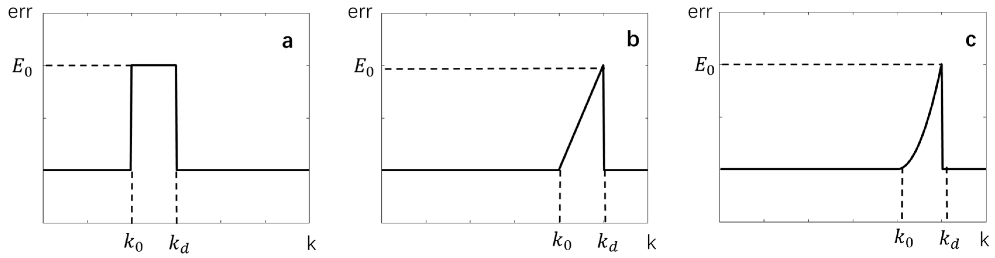
Among these conditions, (1), (2), and (3) are classified as sudden faults, characterized by abrupt and significant deviations in the sensor output. Condition (4) is classified as a gradual fault, wherein the sensor error progressively increases over time.

Assuming that the sensor output signal is denoted during normal operation of the integrated navigation system and under fault conditions, the abnormal behavior of the sensor can be described as follows:

$$B_e(k)=B(k)+err(k)$$

(1)

When a sudden fault occurs,

$$err(k)=\left\{\begin{array}{l}f(k),\hspace{1em}{k}_0\le k<k_d\\ 0,\hspace{1em}{k}_0>k,k\ge k_d\end{array}\right.$$

(2)

where $k_0$ denotes the moment when the fault occurs, and $k_d$ denotes the moment when the fault is resolved.

As shown in Figure 1a, when a sudden fault occurs at $f(k)=E_0$, the value of $E_0$ remains constant. When a gradual fault occurs,

$$err(k)=\left\{\begin{array}{l}S(k-k_0)\hspace{1em}or\hspace{1em}S{(k-k_0)}^2,\hspace{1em}{k}_0\le k<k_d\\ 0,\begin{array}{ccc}{k}_0>k& or& k\ge k_d\end{array}\end{array}\right.$$

(3)

When $err(k)=S(k-k_0)$ occurs, the gradual fault is referred to as a linear gradual fault, as illustrated in Figure 1b, where the sensor fault value demonstrates a linear relationship with fault time. When $err(k)=S{(k-k_0)}^2$ occurs, the fault progression is depicted in Figure 1c, representing a quadratic function gradual fault, where the fault value varies with time according to a quadratic function.

As shown in Figure 1, when a sudden fault occurs, the sensor fault signal undergoes a significant step-change, which serves as a distinguishing characteristic for fault detection. However, when a gradual fault occurs, the sensor fault signal progressively increases over time, particularly in the early stages, where the sensor output error develops at a relatively slow rate. This gradual change complicates the detection process. Therefore, particular emphasis must be placed on detecting gradual faults when conducting fault detection in AUV-integrated navigation systems.

3. The Cumulative Residual Detection Method with Error Coefficient Amplification

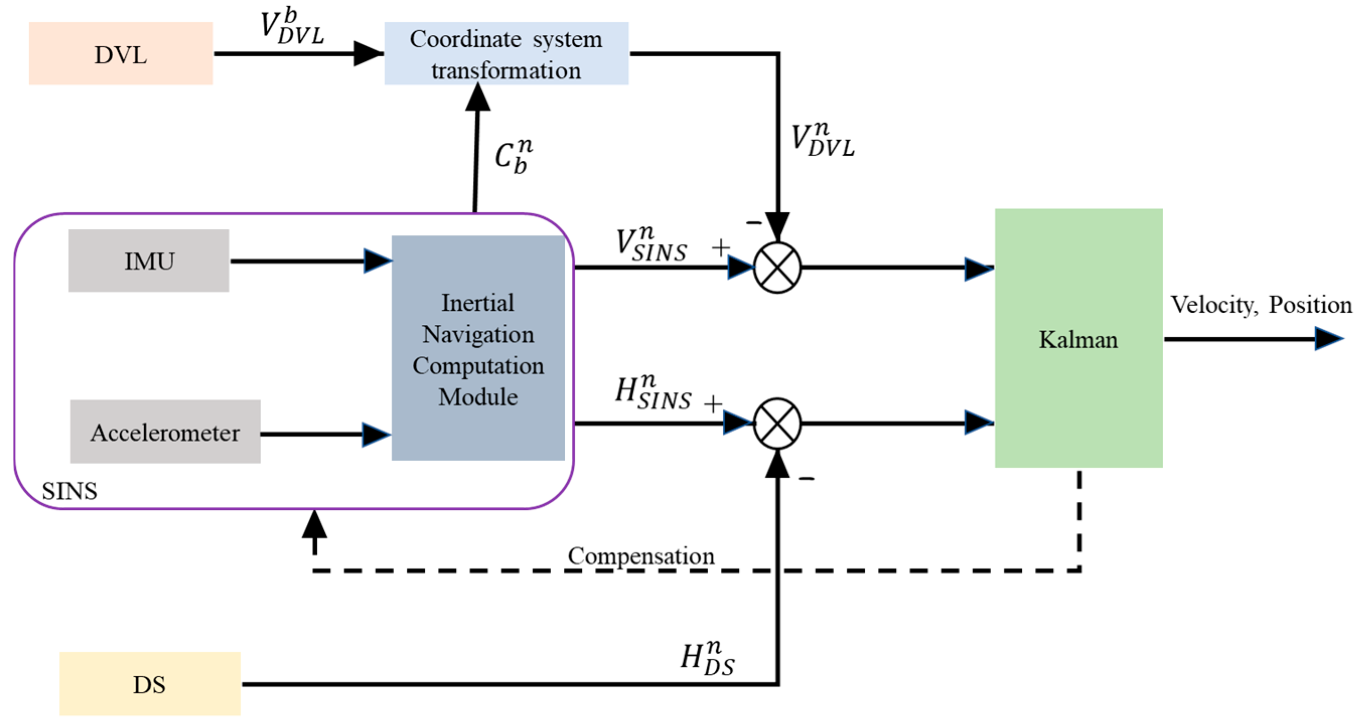
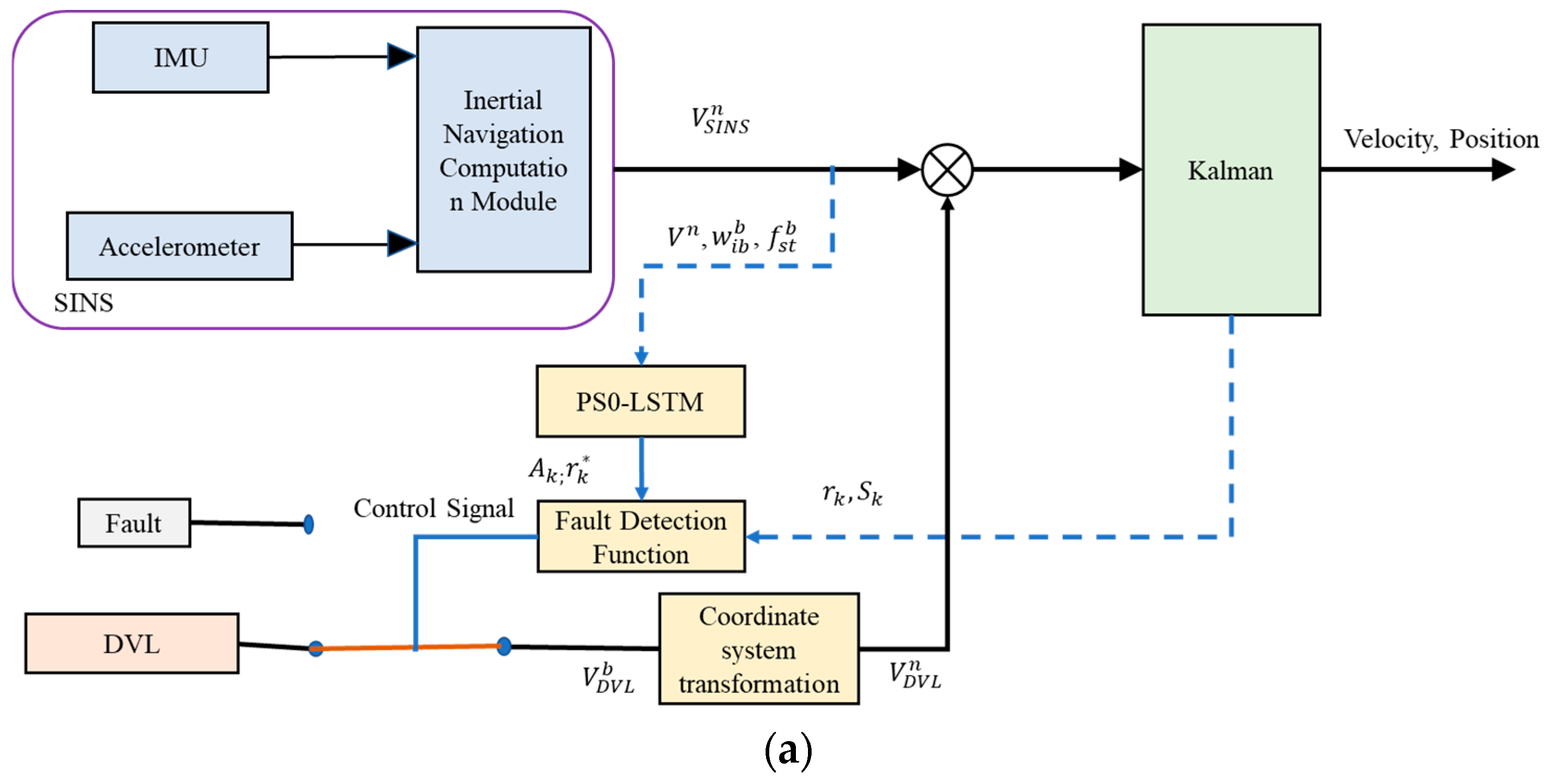
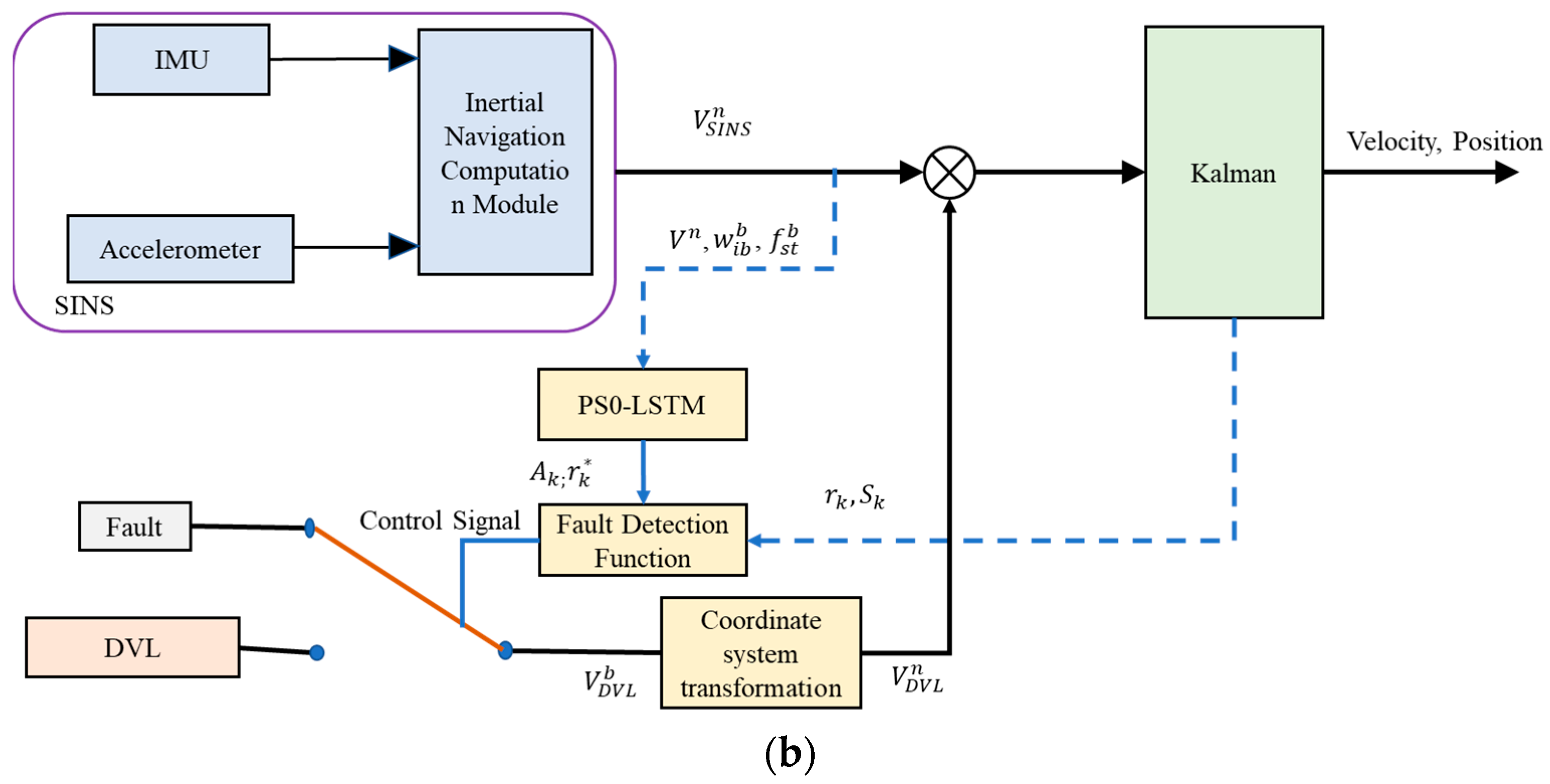
When SINS and the DVL are applied in the loosely integrated navigation model, observations from the DVL comprise velocity measurements of the AUV in the body coordinate system, while the depth sensor (DS) supplies depth data. The loosely integrated model of SINS, DVL, and DS is shown in Figure 2. SINS offers continuous information on velocity, attitude, and position relative to the n-coordinate system. The information collected by the DVL includes three-dimensional velocity measurements in the body coordinate system b, which are transformed into the n-coordinate system using a coordinate transformation matrix. The inputs to the Kalman filter observation equations include the differences between velocity values derived from SINS and the DVL, along with the differences between depth values from SINS and the DS.

In the loosely integrated structure of SINS, DVL, and DS, the selected state variables are as follows.

$$\begin{array}{l}{\mathit{X}}_k=[{\varphi }_x,{\varphi }_y,{\varphi }_z,\delta V_E^n,\delta V_N^n,\delta V_U^n,\delta \lambda ,\delta L,\delta h,{\nabla }_x,{\nabla }_y,{\nabla }_z,{\xi }_x,{\xi }_y,{\xi }_z,\\ \hspace{1em}\hspace{1em} \delta V_{DVL},\delta \Delta ,\delta C,\delta h_{DS}{]}^T\end{array}$$

(4)

where ${\varphi }_x,{\varphi }_y,{\varphi }_z$ denote the attitude angle errors of SINS along the east, north, and up directions, respectively; the unit is radians. Similarly, $\delta V_E^n,\delta V_N^n,\delta V_U^n$ indicate the velocity errors of SINS along the east, north, and up directions; the unit is m/s. $\delta \lambda ,\delta L,\delta h$ represents the errors in latitude, longitude, and depth; the units are radians and meters, respectively. ${\nabla }_x,{\nabla }_y,{\nabla }_z$ denote the constant offset of the accelerometer along the three axes in the body coordinate system, and the unit is $\mathrm{m}/{\mathrm{s}}^2$, while ${\xi }_x,{\xi }_y,{\xi }_z$ denotes the gyro biases along the three axes in the body coordinate system; the unit is radians. Finally, $\delta h_{DS}$ represents the measurement depth error; the unit is m.

For the AUV-integrated navigation system, the state equation and measurement equation in the Kalman filtering process are as follows:

$$\left\{\begin{array}{l}{\mathit{X}}_k={\mathsf{\varphi }}_{k,k-1}{\mathit{X}}_{k-1}+{\mathit{W}}_{k-1}\\ {\mathit{Z}}_k={\mathit{H}}_k{\mathit{X}}_k+{\mathit{V}}_k\end{array}\right.$$

(5)

In the equation, ${\mathsf{\varphi }}_{k,k-1}$, ${\mathit{H}}_k$ is the state transition matrix, and ${\mathit{W}}_{k-1}$, ${\mathit{V}}_k$ is the noise vector. The specific expression of ${\mathsf{\varphi }}_{k,k-1}$, ${\mathit{H}}_k$ can be found in references [22,23].

If the system is fault-free before time $k-1$, then the estimate ${\mathit{X}}_{k-1}$ at time $k-1$ within the Kalman filtering process is considered accurate. According to Equation (5), the system state at time $k$ can be expressed as follows:

$${\widehat{\mathit{X}}}_{k,k-1}={\mathsf{\varphi }}_{k,k-1}{\widehat{\mathit{X}}}_{k-1}$$

(6)

The predicted measurement value of the system at time $k$ is

$${\widehat{\mathit{Z}}}_{k,k-1}={\mathit{H}}_k{\widehat{\mathit{X}}}_{k,k-1}$$

(7)

The innovation, also known as the residual, in the Kalman filtering process is defined as the difference between ${\mathit{Z}}_k$ and ${\widehat{\mathit{Z}}}_{k,k-1}$, and can be expressed as follows:

$${\mathit{r}}_k={\mathit{Z}}_k-{\widehat{\mathit{Z}}}_{k,k-1}$$

(8)

According to Kalman filtering theory, when the system is fault-free, the residual ${\mathit{r}}_k$ is characterized as zero-mean Gaussian white noise. Therefore, the variance can be expressed as follows:

$${\mathit{S}}_k={\mathit{H}}_k{\mathit{P}}_{k,k-1}{\mathit{H}}_k^T+{\mathit{r}}_k$$

(9)

When a fault occurs in the system, the residual mean deviates from zero. Therefore, this characteristic can be utilized to monitor the residual and assess the operational status of the system.

In integrated navigation systems, the residual chi-square detection method [24,25] is widely utilized for its simplicity and effectiveness in detecting significant fault information. The core of this method involves computing the filter innovation and residuals, excelling at detecting sudden faults. However, when a gradual fault occurs, the changes in the early stages are subtle and challenging to detect. Consequently, the residual chi-square detection method is not effective in identifying gradual faults. To overcome this limitation, this paper proposes a cumulative residual detection method with error coefficient amplification based on the concept of cumulative sum.

Cumulative sum (CUSUM) is a statistical concept originally proposed by Page in 1954, with its fundamental principle being the continuous accumulation of data-derived information [26]. When the data exhibits small changes, the CUSUM algorithm amplifies these subtle changes through the cumulative process, thereby increasing the significance of the outcomes.

Under normal system conditions, the probability distribution of the residual is $P_0(r_k)$. In the presence of a fault, the probability distribution of the residual becomes $P_1(r_k)$, and the logarithmic likelihood ratio of the residual probability distribution, $f(r_k)$ is expressed as follows:

$$f(r_k)={\log }_e{\displaystyle \frac{P_1(r_k)}{P_0(r_k)}}$$

(10)

Let the initial value of the cumulative sum be $F_0=0$; then, the CUSUM is

$$F_k=\left\{\begin{array}{cc}\hfill 0,& F_{k-1}+f({\mathit{r}}_k)<0\hfill \\ \hfill F_{k-1}+f({\mathit{r}}_k),& F_{k-1}+f({\mathit{r}}_k)\ge 0\hfill \end{array}\right.$$

(11)

In practice, $P_0(r_k)$ and $P_1(r_k)$ may be unknown parameters, and their calculation can be complex.

The non-parametric CUSUM algorithm operates under the assumption that, under normal conditions, the mean of the random variable is negative and exhibits a tendency to shift toward positive values [27]. The non-parametric CUSUM is constructed without losing any statistical properties. Under typical conditions, the mean of the random sequence is assumed to be biased toward negative values but exhibits a positive trend. To replace the above $f({\mathit{r}}_k)$, $m(k)$ is proposed.

$$m(k)=‖{\mathit{r}}_k‖-\beta$$

(12)

Let $m(k)$ represent the detection sequence in the CUSUM algorithm, with $\beta$ defined as a constant. When the system is fault-free, Equation (12) is negative; therefore, the mean value $E(m(k))$ of $m(k)$ must be less than zero. To ensure that $E(m(k))$ is less than zero, the value of $\beta$ must be determined according to the operational conditions of the integrated navigation system and is typically defined as a constant. Assuming the system’s residual is $\sigma$, the value of $\beta$ can be set near $3\sigma$, ensuring that the majority of $m(k)$ values remain below zero. Equation (11) can then be transformed into Equation (13).

$$F_k=\left\{\begin{array}{cc}\hfill 0,& F_{k-1}+m(k)<0\hfill \\ \hfill F_{k-1}+m(k),& F_{k-1}+m(k)\ge 0\hfill \end{array}\right.$$

(13)

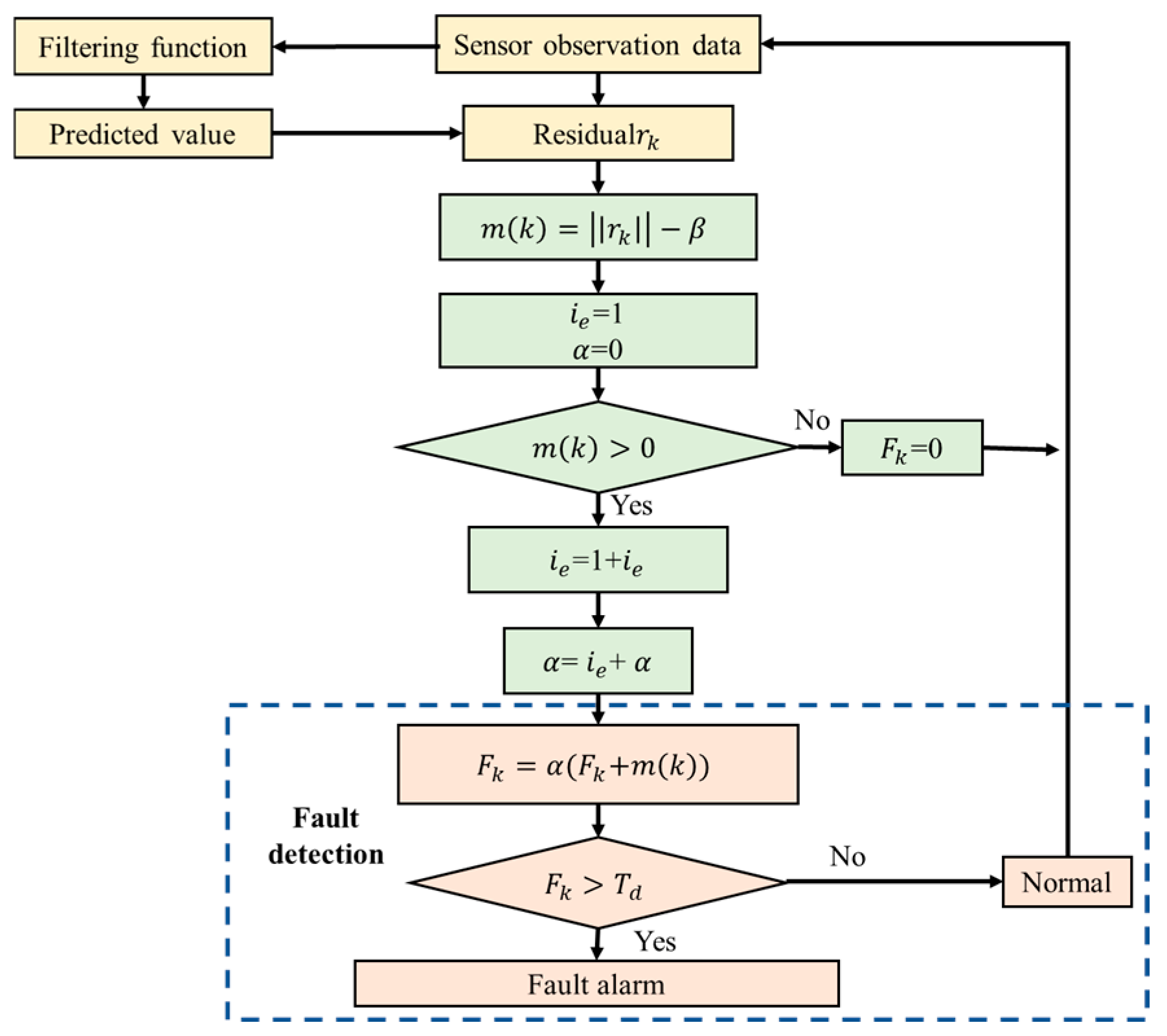
As analyzed in Section 2 regarding the causes of faults, the initial errors in gradual faults are typically small, leading to a slow accumulation of changes in the $F_k$ process within the CUSUM algorithm. To enhance the CUSUM algorithm’s capability to detect gradual faults, an error amplification coefficient $\alpha$ has been incorporated into the original CUSUM algorithm.

$$\begin{array}{l}\alpha =0\\ \chi =\alpha +i_e\\ \alpha =\chi \end{array}$$

(14)

where $\alpha$ starts with an initial value of 0, $i_e$ denotes the count of abnormal occurrences for $F_k$, and its initial value is set to 1.

$$F_k=\left\{\begin{array}{cc}\hfill 0,& F_{k-1}+m(k)<0\hfill \\ \hfill \alpha (F_{k-1}+m(k)),& F_{k-1}+m(k)\ge 0\hfill \end{array}\right.$$

(15)

Set the detection threshold $T_d$.

$$\left\{\begin{array}{l}\mathrm{Error}:F_k>T_d\\ \mathrm{Normal}:F_k\le T_d\end{array}\right.$$

(16)

The fault detection threshold $T_d$ must be carefully adjusted to strike a balance between the false alarm rate and the missed detection rate. The false alarm rate is defined as the probability of an incorrect fault indication in the absence of an actual fault, whereas the missed detection rate denotes the probability of failing to identify a fault when one is present. An excessively high detection threshold tends to result in a higher missed detection rate; conversely, a threshold that is too low increases the likelihood of false alarms.

The detailed procedure of the cumulative residual fault detection method with error coefficient amplification is illustrated in Figure 3.

4. Fault Detection Method Based on PSO-LSTM

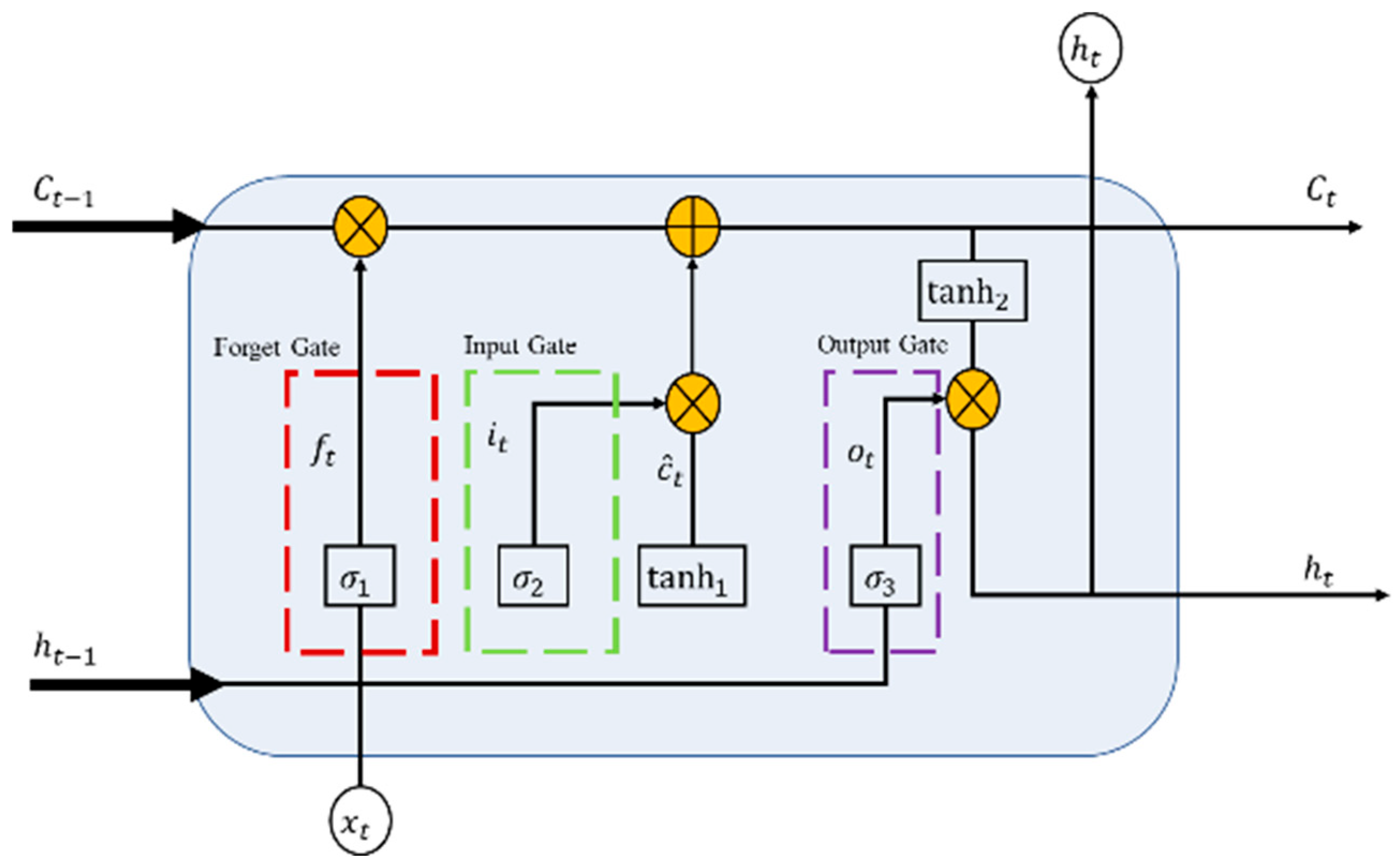
LSTM networks were first proposed by Hochreiter et al. [28]. The network is characterized by three gate structures, providing the hidden layers with a more complex architecture. This design allows LSTM to learn the features of input signals more easily. As shown in Figure 4, a standard LSTM module is primarily composed of an input gate, an output gate, and a forget gate [29,30].

(1)

Input Gate $i_t$

The input gate is utilized to introduce the latest data and regulates the extent of data integration. Let $x_t$ denote the signal entering at time $\mathit{t}$, $h_t$ the output at time $\mathit{t}$, and $W_t$ the weight associated with the output gate, while $b_i$ represents the bias of the input gate. The result $i_t$ for the input gate is expressed as follows:

$$i_t=\sigma (W_i\ast [h_{t-1},x_t]+b_i)$$

(17)

(2)

Forget Gate $f_t$

The forget gate is utilized to regulate the stored information. Information meeting specific criteria is retained, while information failing to meet the criteria is discarded and excluded from further processing. The expression for the forget gate is as follows:

$$f_t=\sigma (W_f\ast [h_{t-1},x_t]+b_f)$$

(18)

(3)

Output Gate $O_t$

The output gate is utilized to determine the unit state to be output. It is governed by the input signal $x_t$ at time $\mathit{t}$ and the output $h_{t-1}$ from the hidden layer’s previous time step. The expression for the output gate is as follows:

$$O_t=\sigma (W_o\ast [h_{t-1},x_t]+b_o)$$

(19)

In the equation, $W_o$ is the weight of the input gate, and $b_o$ is the bias of the input gate.

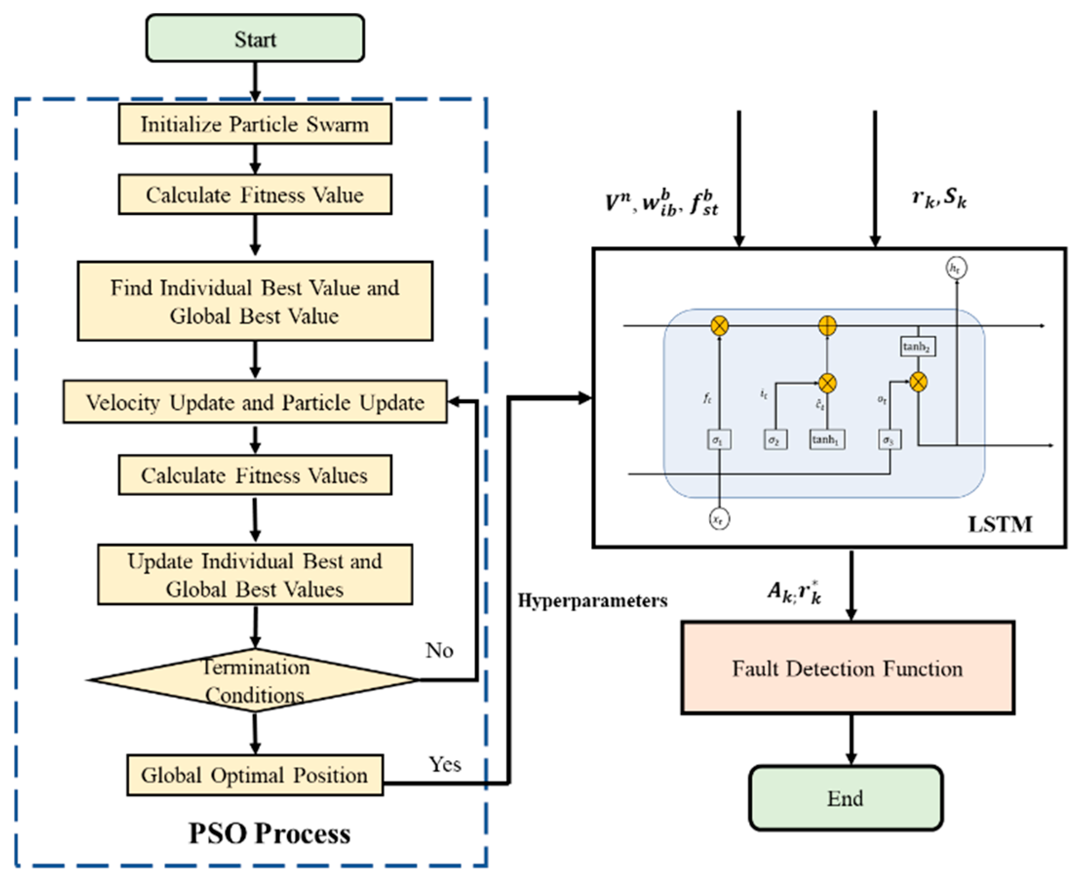
As shown in Figure 5, the fault detection method based on LSTM comprises two primary stages: model training and fault detection. Typically, constructing an efficient deep learning model is complex and time-consuming, requiring the determination of model structure and hyperparameters, such as batch size and learning rate, both of which have a substantial impact on model performance. The goal of hyperparameter optimization is to identify the optimal parameters that align with the model’s requirements. However, for complex models, determining the appropriate hyperparameters often poses a significant challenge. In this study, the PSO algorithm has been employed to optimize the LSTM hyperparameters, with the objective of enhancing the performance of the error detection model [31].

In the model training phase, the PSO-LSTM model is trained on the Kalman filter’s innovation and variance obtained under normal operating conditions of the integrated navigation system, along with the sensor data from the SINS. In the fault detection phase, the trained LSTM model is employed to predict the innovation and variance based on the SINS sensor data. The LSTM-predicted results are then compared with the Kalman filter’s innovation and variance and subsequently input into the fault detection function to evaluate the system status and generate corresponding control signals. Using Equations (8) and (9), the Kalman filter’s innovation ${\mathit{r}}_k$ and variance ${\mathit{S}}_k$, as well as the LSTM-predicted innovation ${\mathit{r}}_k^{*}$ and variance ${\mathit{A}}_k$, are derived.

The LSTM algorithm is effective in capturing temporal dependencies and nonlinear dynamic features in time series and is capable of learning the long-term operational patterns of integrated navigation systems. The Kalman filter algorithm is capable of providing real-time state estimation and effectively suppressing Gaussian noise. PSO is a global optimization algorithm that facilitates the optimization of model parameters to enhance overall performance. The fusion of these methods enables simultaneous exploitation of LSTM’s memory capability, KF’s noise suppression, and PSO’s optimization strength, thereby improving the overall accuracy of the model.

Before the LSTM model can be used to predict innovation and variance, the model must undergo training, as shown in Figure 6. During the training process of the LSTM fault detection model, two primary processes are involved: the selection of hyperparameters and the determination of input feature parameters. To improve the efficiency of model training, a PSO algorithm is employed to optimize the hyperparameter selection for the LSTM prediction model. In the selection of feature parameters, the feature parameters from the fault-free integrated navigation system are chosen as both the input and output features of the model. For the output, the innovation from the fault-free Kalman filter system is designated as the model’s output sample. As for the input features, three primary input features are currently identified:

• The velocity output from the SINS serves as the training sample.
• The attitude, position, velocity, and specific force outputs from the SINS constitute the input samples.
• The incremental errors of attitude, velocity, position, and specific force from the SINS are selected as the training samples.

For artificial intelligence algorithms, the number of input training variables influences both the model’s training speed and the accuracy of its output. Therefore, careful selection of model inputs is essential. In the integrated navigation system, the velocity of the AUV at a certain moment is represented as follows [32]:

$${\mathit{V}}^n={\tilde{\mathit{V}}}^n+\Delta {\mathit{V}}_{sf}^n+\Delta {\mathit{V}}_{cor/g}^n$$

(20)

where ${\tilde{\mathit{V}}}^n$ represents the velocity at the previous time step, and $\Delta {\mathit{V}}_{sf}^n$ and $\Delta {\mathit{V}}_{cor/g}^n$ can be expressed as follows:

$$\begin{array}{l}\Delta {\mathit{V}}_{sf}^n={\mathit{C}}_b^n\Delta {\mathit{V}}_k-{\displaystyle \frac{1}{2}}{\mathit{w}}_{in}^n\times {\mathit{T}}_b^n\Delta \mathit{v}\\ \hspace{1em}\hspace{1em} +{\mathit{C}}_b^n({\displaystyle \frac{1}{2}}\Delta \mathsf{\theta }\times \Delta \mathit{v}+{\displaystyle \frac{1}{2}}\Delta \mathsf{\theta }\times {\mathit{f}}_{st}^b+\Delta {\mathit{V}}_k\times {\mathit{w}}_{ib}^b)\\ \hspace{1em}\hspace{1em} \Delta {\mathit{V}}_{cor/g}^n=-\left[2{\mathit{w}}_{ie}^n+{\mathit{w}}_{en}^n\right]\times {\mathit{V}}^n+{\mathit{g}}^n\end{array}$$

(21)

where ${\mathit{w}}_{ie}^n$ represents the Earth’s angular velocity, ${\mathit{w}}_{en}^n$ represents the angular velocity of the n-frame relative to the e-frame, and ${\mathit{w}}_{in}^n={\mathit{w}}_{ie}^n+{\mathit{w}}_{en}^n$, ${\mathit{w}}_{ib}^b$ and ${\mathit{f}}_{st}^b$ represent the angular velocity and specific force in the b-frame. $\Delta \mathsf{\theta }$ and $\Delta \mathit{v}$ represent the discrete integrals of the gyroscope and accelerometer over a brief time interval, and they can be expressed as follows:

$$\begin{gathered} \Delta \mathsf{\theta }={\displaystyle \int {\mathit{w}}_{ib}^{b}dt} \\ \Delta v={\displaystyle \int {\mathit{f}}_{st}^{b}dt} \end{gathered}$$

(22)

From the above analysis, it is evident that the speed of the AUV is primarily influenced by the velocity, angular velocity, specific force, and attitude angles of the inertial navigation system. Therefore, these parameters are chosen as the input features for the LSTM model. The root mean square error (RMSE) is defined as the fitness function for the PSO. The hyperparameters of the LSTM model are optimized using PSO. Once the LSTM model is trained, it acquires the ability to make predictions. By using the velocity, angular velocity, specific force, and attitude angles of the inertial navigation system as inputs, the corresponding Kalman filter residuals ${\mathit{r}}_k^{*}$ and their variances ${\mathit{A}}_k$ are predicted.

In the LSTM model, define variable ${\mathit{L}}_k$ as follows:

$${\mathit{L}}_k={\mathit{r}}_k-{\mathit{r}}_k^{*}$$

(23)

Since the innovation ${\mathit{r}}_k$ and the LSTM-predicted innovation ${\mathit{r}}_k^{*}$ are independent of each other, the variance of ${\mathit{L}}_k$ is given by the following:

$${\mathit{A}}_k={\mathit{S}}_k+\mathrm{cov}(r_k^{*})$$

(24)

If the system is operating normally, the signal ${\mathit{L}}_k$ is expected to exhibit zero-mean Gaussian white noise properties. However, if the system experiences an anomaly, the mean of signal ${\mathit{L}}_k$ deviates from zero. For the signal ${\mathit{L}}_k$, two opposing hypotheses are defined as follows:

$$\left\{\begin{array}{l}{\mathrm{H}}_0(\mathrm{Normal}):E({\mathit{L}}_k)=0,E({\mathit{L}}_k{\mathit{L}}_k^T)={\mathit{A}}_k\\ {\mathrm{H}}_1(\mathrm{Error}):E({\mathit{L}}_k)=\mathsf{\mu },E(({\mathit{L}}_k-\mathsf{\mu }){(L_k-\mathsf{\mu })}^T)={\mathit{A}}_k\end{array}\right.$$

(25)

The following probability density functions are then defined:

$$P_r(L|H_0)={\displaystyle \frac{1}{\sqrt{2\pi ·\left|{\mathit{A}}_k\right|}}}\exp (-{\displaystyle \frac{1}{2}}{\mathit{L}}_k^T{\mathit{A}}_k^{-1}{\mathit{L}}_k)$$

(26)

$$P_r(L|H_1)={\displaystyle \frac{1}{\sqrt{2\pi ·\left|{\mathit{A}}_k\right|}}}\exp (-{\displaystyle \frac{1}{2}}{({\mathit{L}}_k-\mathsf{\mu })}^T{\mathit{A}}_k^{-1}({\mathit{L}}_k-\mathsf{\mu }))$$

(27)

where $\left|{\mathit{A}}_k\right|$ represents the determinant of matrix ${\mathit{A}}_k$.

The Neyman-Pearson theorem states that among tests conducted at the same significance level, the likelihood ratio test achieves the highest statistical power. Therefore, the log-likelihood ratio between $P_r(L|H_1)$ and $P_r(L|H_0)$ can be calculated.

$${\Lambda }_k=\ln {\displaystyle \frac{P_r(L|H_1)}{P_r(L|H_0)}}={\displaystyle \frac{1}{2}}\left[{\mathit{L}}_k^T{\mathit{A}}_k^{-1}{\mathit{L}}_k-{({\mathit{L}}_k-\mathsf{\mu })}^T{\mathit{A}}_k^{-1}({\mathit{L}}_k-\mathsf{\mu }))\right]$$

(28)

When $\mathsf{\mu }={\mathit{L}}_k$ is reached, the log-likelihood ratio ${\mathbf{\Lambda }}_k$ reaches its maximum value. Therefore, the fault detection function (FDF) based on the LSTM model is defined as follows:

$$F_k={\mathit{L}}_k^T{\mathit{A}}_k^{-1}{\mathit{L}}_k={({\mathit{r}}_k-{\mathit{r}}_k^{*})}^T{\left[\mathrm{cov}({\mathit{r}}_k)+\mathrm{cov}({\mathit{r}}_k^{*})\right]}^{-1}({\mathit{r}}_k-{\mathit{r}}_k^{*})$$

(29)

When the system experiences an abnormal condition, the noise ${\mathit{L}}_k$ no longer exhibits zero-mean Gaussian white noise properties, resulting in an intensified signal $F_k$. This change can serve as the basis for fault diagnosis, with the specific detection criterion as follows:

$$\left\{\begin{array}{l}\mathrm{Normal}:\hspace{1em}{F}_k\le T_d\\ \mathrm{Error}:\hspace{1em}{F}_k>T_d\end{array}\right.$$

(30)

where $T_d$ is the detection threshold.

Based on the aforementioned modeling process, it can be inferred that the proposed PSO-LSTM fault detection method is theoretically feasible. First, LSTM networks possess strong capabilities for modeling time series data and are able to capture the nonlinear dynamic behavior of integrated navigation systems with adequate training. Second, the PSO algorithm is capable of effectively optimizing the network architecture and parameters of the LSTM, thereby enhancing its prediction accuracy. Finally, by statistically analyzing the predicted residuals, statistically significant differentiation can be achieved in the presence of faults. Therefore, at the theoretical level, this method is theoretically capable of achieving a high-precision and robust fault detection capability for integrated navigation systems.

5. Verification and Analysis

To verify the feasibility of the proposed algorithm, experimental data, gathered by the underwater robot Snapir from a designated sea area, were utilized for validation [33]. The underwater robot Snapir is outfitted with various sensors, such as the VN-100 inertial navigation component, DVL, depth sensor, and hydrophone. The fault detection experiment employed a combined navigation system, comprising the inertial navigation component and DVL, to evaluate the fault detection algorithm’s effectiveness. The key sensor parameter information is provided in

Table 1. Main parameters of the sensor.

Sensor	Parameter	Parameter Value
IMU	Bias Stability	<${10}^{°}$/h
	Noise Density	${0.0035}^{°}/\mathrm{s}/\sqrt{\mathrm{H}\mathrm{z}}$
	Bias Error	${\pm 0.05}^{°}$
Accelerometer	Bias Stability	<$0.04 \mathrm{m}\mathrm{g}$
	Noise Density	$0.14 \mathrm{m}\mathrm{g}/\sqrt{\mathrm{H}\mathrm{z}}$
	Bias Error	${\pm 0.05}^{°}$
DVL	Velocity Range	$\pm 10 \mathrm{m}/\mathrm{s}$
	Velocity Resolution	$0.1 \mathrm{c}\mathrm{m}/\mathrm{s}$

.

5.1. Analysis of the Detection Performance of the Cumulative Residual Error Detection Method with Error Coefficient Amplification

To analyze the fault detection performance of the cumulative residual error detection method with error coefficient amplification, experimental data collected over 6000 s by an underwater robot were analyzed. Considering both the false alarm rate and the missed detection rate, the amplification factor $\beta$ of the cumulative residual error detection method was set to 0.3, with the corresponding detection threshold $T_d$ set to 0.2. Additionally, the detection threshold $T_d$ in the residual chi-square detection method was set to 18. Fault detection capabilities were compared by introducing diverse fault scenarios into 6000 s of experimental data collected by an underwater robot.

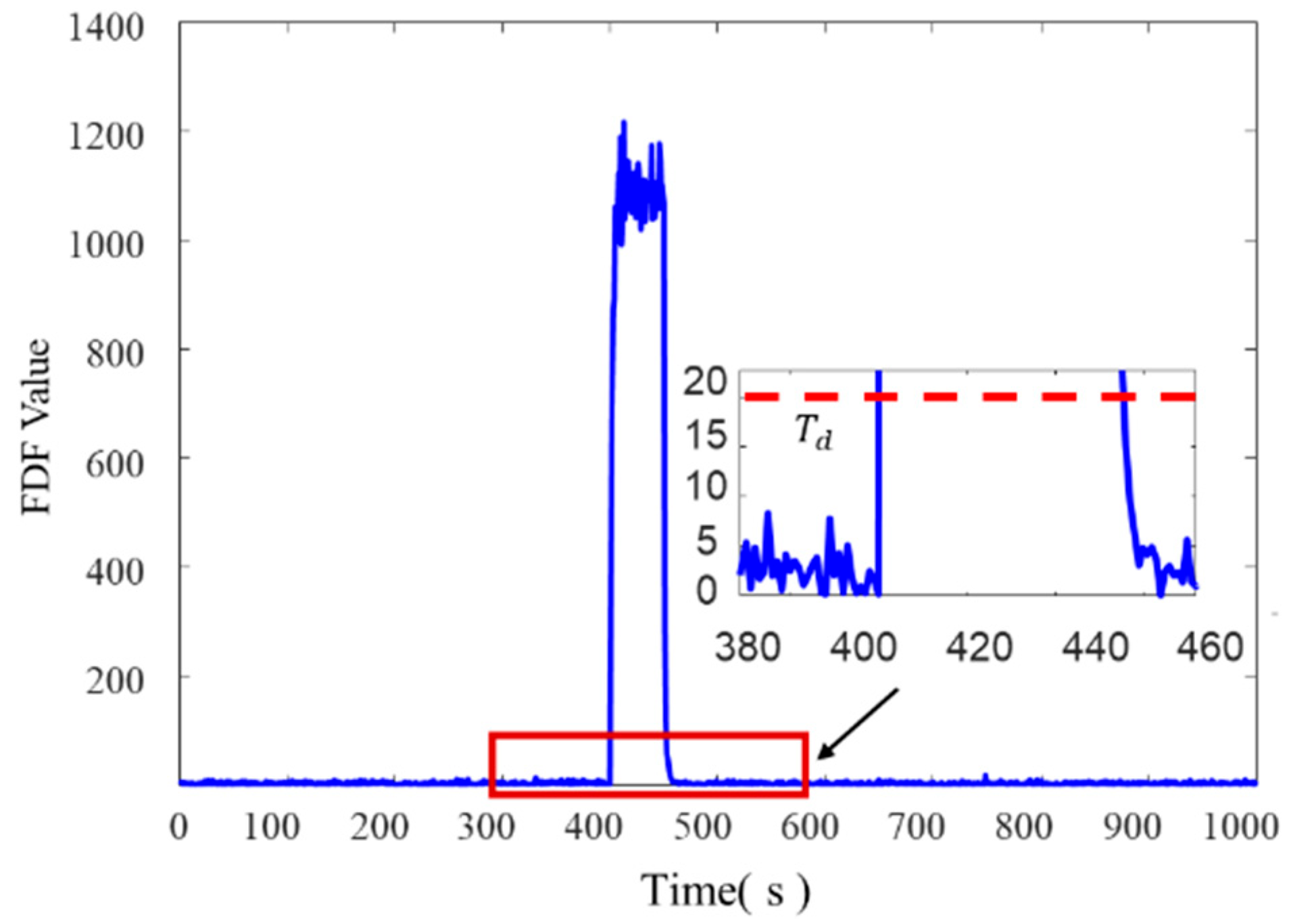
In the detection of sudden faults in the integrated navigation system, a sudden fault of 1 m/s was introduced into DVL experimental data between 400 and 450 s, with the fault detection results presented in Figure 7 and Figure 8. Due to the sudden increase in the data collected by the DVL, the FDF values for both fault detection methods exhibited rapid and significant variations. Both methods successfully detected the fault at 400 s, indicating strong capabilities of both methods for detecting sudden faults.

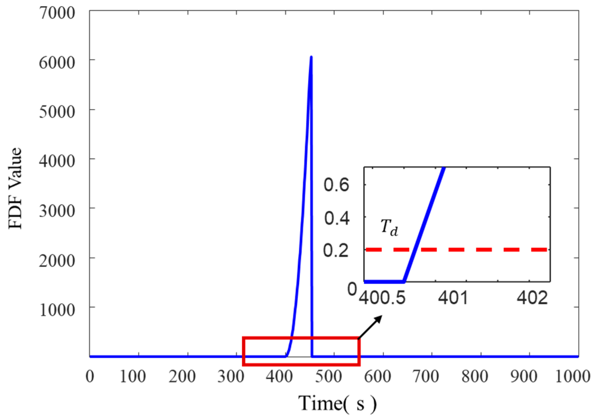
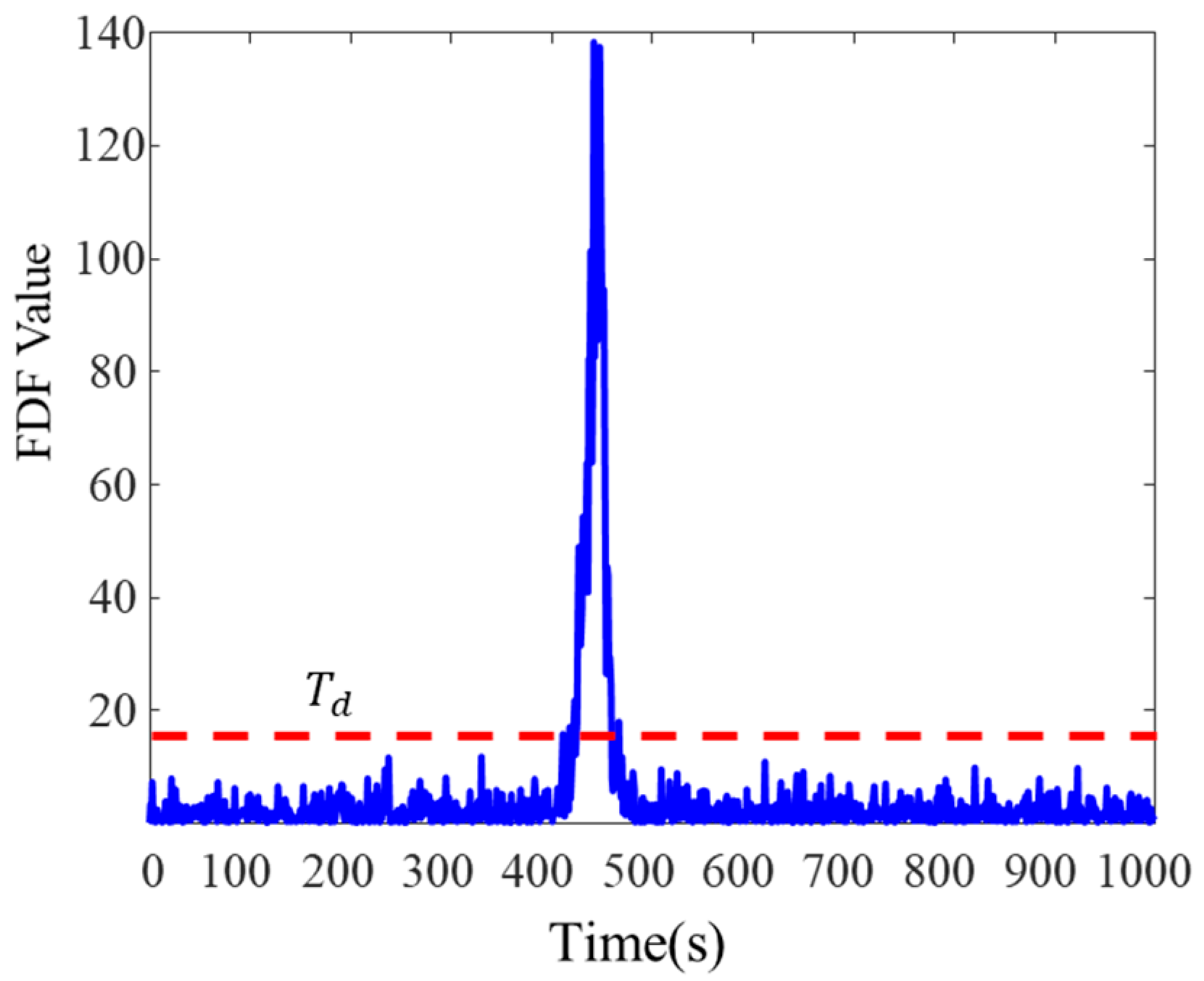
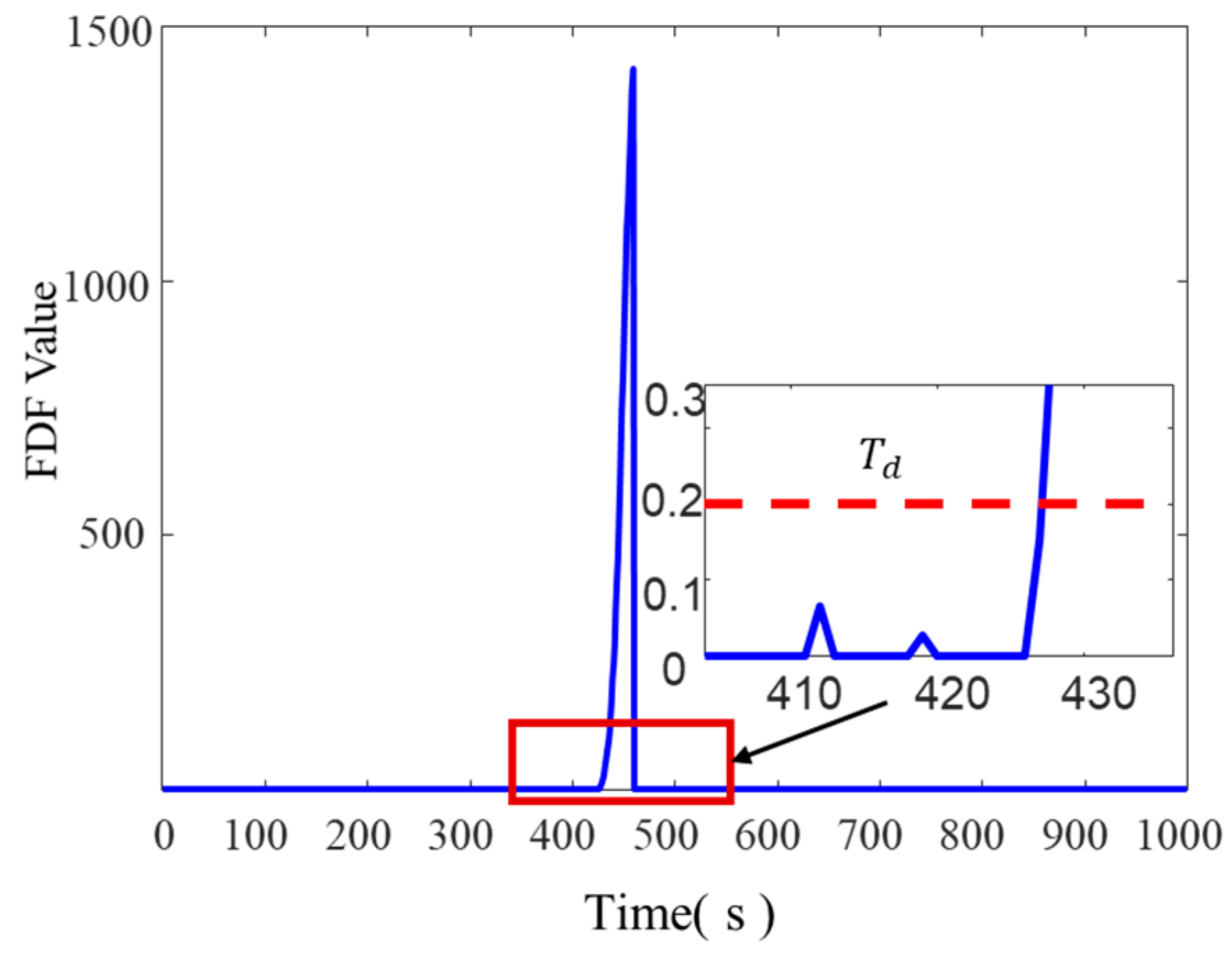
The performance of the integrated navigation system in detecting gradient-type faults was evaluated by introducing a simulated linear gradient fault into the DVL data between 400 s and 450 s. The fault detection capabilities of two algorithms were evaluated, with the corresponding results presented in Figure 9 and Figure 10. Compared to sudden faults, both methods demonstrated lower sensitivity in identifying gradual deviations. The residual chi-square detection method identified the fault at 434 s, while the error coefficient amplification cumulative residual detection method identified it earlier at 427 s, indicating improved responsiveness. These results suggest that the proposed error coefficient amplification cumulative residual detection algorithm provides enhanced performance in identifying slowly varying faults in navigation sensor data.

To further compare the fault detection capabilities of the two methods for gradient faults, a $f=0.001\times (t-t_e)$ linear gradient fault, lasting 50 s, was introduced into the DVL data at intervals of 100 s throughout the 6000 s experimental dataset, where $t_e$ represents the fault occurrence time. Through the incorporation of fault data into the DVL, 40 fault segments and 40 fault-free segments were generated in the integrated navigation system. During fault-free periods, data from the acoustic positioning system was employed to compensate for accumulated errors caused by the inertial navigation unit during fault occurrences, ensuring that each fault segment began under stable fault conditions. The final false alarm and missed detection results for both the error coefficient amplification cumulative residual detection method and the residual chi-square detection method are presented in

Table 2. Comparison of detection results.

Fault Detection Method	False Alarm Rate (%)	Missed Detection Rate (%)
Residual Chi-Square Detection Method	7.5	37.5
Amplified Error Coefficient Cumulative Residual Detection Method	5	12.5

.

As shown in Table 2, the false alarm rate and missed detection rate of the residual chi-square detection method exceed those observed in the error coefficient amplification cumulative residual detection method. Specifically, the false alarm rate of the residual chi-square detection method exceeds that of the error coefficient amplification cumulative residual detection method by 2%, and its missed detection rate exceeds it by 25%. This discrepancy is primarily attributed to the detection threshold of the residual chi-square detection method, which is substantially higher than that of the error coefficient amplification cumulative residual detection method, thereby reducing its detection capability for gradient faults. Additionally, differences in FDF values, as illustrated in Figure 8 and Figure 9, indicate that the error coefficient amplification cumulative residual detection method, through the construction of a non-parametric β value, ensures that, during stable operation of the integrated navigation system, the FDF value remains less than or equal to 0, thereby mitigating an increase in the false alarm rate caused by a small calibration threshold. In terms of FDF value variation, the error coefficient amplification cumulative residual detection method effectively amplifies gradient fault values through the use of an error amplification factor associated with the number of faults, producing an FDF value that is substantially higher than that of the residual chi-square method. This amplification enhances its detection capability for gradient faults and reduces the missed detection rate.

In terms of computational complexity, the cumulative residual detection method with error coefficient amplification does not require complex computations, and the internal storage parameters are reset during each iteration. Simulation results indicate that, under the same computational environment, this method exhibits comparable computation time to the chi-square detection method.

From the above analysis, it is concluded that the error coefficient amplification fault detection method demonstrates superior performance compared to the residual fault detection method. However, both methods are based on analytical models that depend on model parameters and the adjustment of function thresholds based on experimental data. Consequently, challenges arise in defining appropriate thresholds for unknown scenarios during the operation of integrated navigation systems. Accordingly, the subsequent section will emphasize intelligent detection algorithms.

5.2. Analysis of the Fault Detection Performance of the PSO-LSTM Fault Detection Method

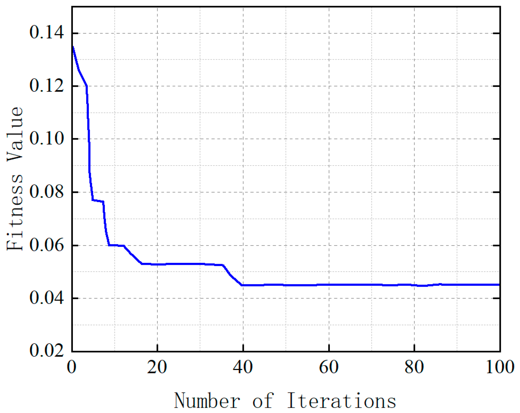
To construct the PSO-LSTM fault detection model, the innovation ${\mathit{r}}_{\mathit{k}}$ and variance ${\mathit{S}}_{\mathit{k}}$ of the 6000 s experimental dataset collected by the underwater robot Snapir under normal operating conditions were computed, where 80% of the data was allocated for training, and the remaining 20% was allocated for validation. The activation function of the fully connected layer in the LSTM model is LeakyReLU, and the loss function employed is the Mean Squared Error (MSE). Additionally, the learning rate decay factor for the LSTM model is set to 0.5. The population size for the PSO algorithm is set to 20, and the training dataset is utilized to optimize the PSO-LSTM model. The fitness function for the PSO algorithm is defined as the root mean square error of the predictions. The PSO algorithm parameters are set as follows: the inertia weight is 0.6, with the learning factors $c_1$ and $c_2$ both set to 2, and the optimization process comprises 100 iterations. The optimization targets the three core parameters of the LSTM model: learning rate, the number of neurons in the hidden layer, and the total number of iterations.

Figure 11 illustrates the iterative process for optimizing LSTM hyperparameters through the PSO algorithm. The stabilization of the fitness value after the 40th iteration suggests that the optimization algorithm has likely converged to a near-optimal solution. At this stage, the particle swarm exhibits minimal variation in fitness improvement across successive iterations, indicating that the search process has approached a local or global optimum in the solution space. Further iterations yield diminishing returns, reflecting a balance between exploration and exploitation. Thus, the learning rate is set to 0.01, and the number of hidden neurons is determined to be 128.

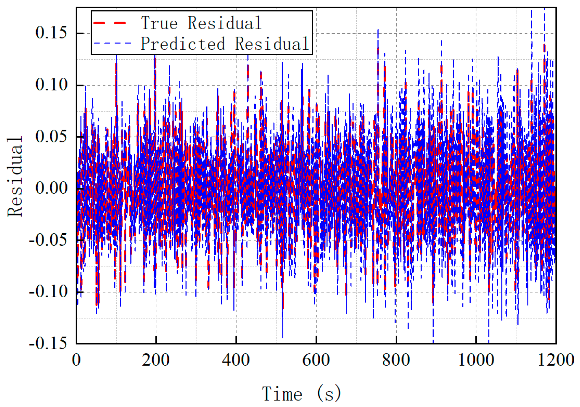
The LSTM model was trained using the hyperparameters optimized by the PSO algorithm, and its prediction results on the test set are presented in Figure 12. As shown in Figure 12, the predicted residuals produced by the trained model are in close agreement with the actual residuals derived from the test set, with both sets exhibiting a consistent temporal trend. The high degree of overlap between the two curves suggests that the model has successfully captured the temporal and statistical characteristics of the residual signal during training. This close alignment not only demonstrates the model’s accuracy in reproducing system behavior under nominal conditions but also indicates its strong generalization capability to previously unseen data. The consistency in both amplitude and phase of the residuals further supports the suitability of the model for reliable anomaly or fault detection in practical navigation scenarios.

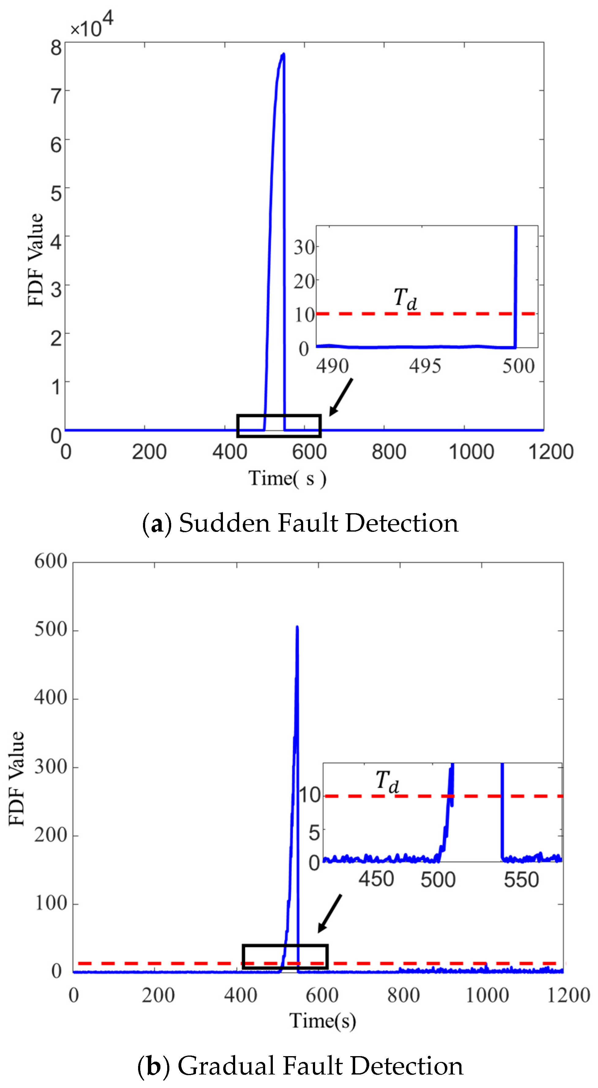
To evaluate the fault detection capability of the PSO-LSTM model for both abrupt and gradual faults, the detection threshold is set to $T_d$ = 10. During the 400–450 s interval of the validation set’s DVL sensor data, a 1 m/s abrupt fault and a gradual linear fault of $f=0.001\times (t-400)$ were introduced. The fault detection results, as reflected by the FDF values, are presented in Figure 13.

As shown in Figure 13, when an abrupt fault occurs in the integrated navigation system, the FDF value associated with the PSO-LSTM fault detection method exhibits a significant increase, enabling the detection of the fault at 400 s, similar to the residual chi-square and error coefficient-amplified cumulative residual methods. When a gradual fault occurs in the integrated navigation system, the PSO-LSTM fault detection method demonstrates a greater variation in FDF values relative to the residual chi-square method. This improvement enhances its capacity to detect gradual faults, allowing the PSO-LSTM method to identify the fault at 17 s.

To further validate the performance and applicability of the PSO-LSTM fault detection method, an additional 1000 s dataset, collected by the underwater robot Snapir in the same water area, was utilized. Fault data from

Table 3. Simulated fault parameters of the DVL system.

No.	Fault Time Interval (s)	Fault Value (m/s)	Fault Type
1	100–120	1	Sudden Fault
2	150–200	0.001 × $\left(\mathrm{t}-150\right)$	Gradual Fault
3	300–350	0.001 × $\left(\mathrm{t}-300\right)$	Gradual Fault
4	500–600	0.001 × $\left(\mathrm{t}-500\right)$	Gradual Fault
5	700–800	0.001 × $\left(\mathrm{t}-700\right)$	Gradual Fault
6	900–1000	0.001 × $\left(\mathrm{t}-900\right)$	Gradual Fault

was introduced into the DVL of the SINS/DVL-integrated navigation system for simulation experiments, comparing the PSO-LSTM model with the residual chi-square and error coefficient-amplified cumulative residual methods in detecting gradual faults. Since the experimental data were collected in the same water area, the detection thresholds for all methods were uniformly set as previously defined. During the fault detection effectiveness testing, when a fault is detected in the integrated navigation system, fault isolation is conducted, leveraging the underwater acoustic positioning data from the Snapir.

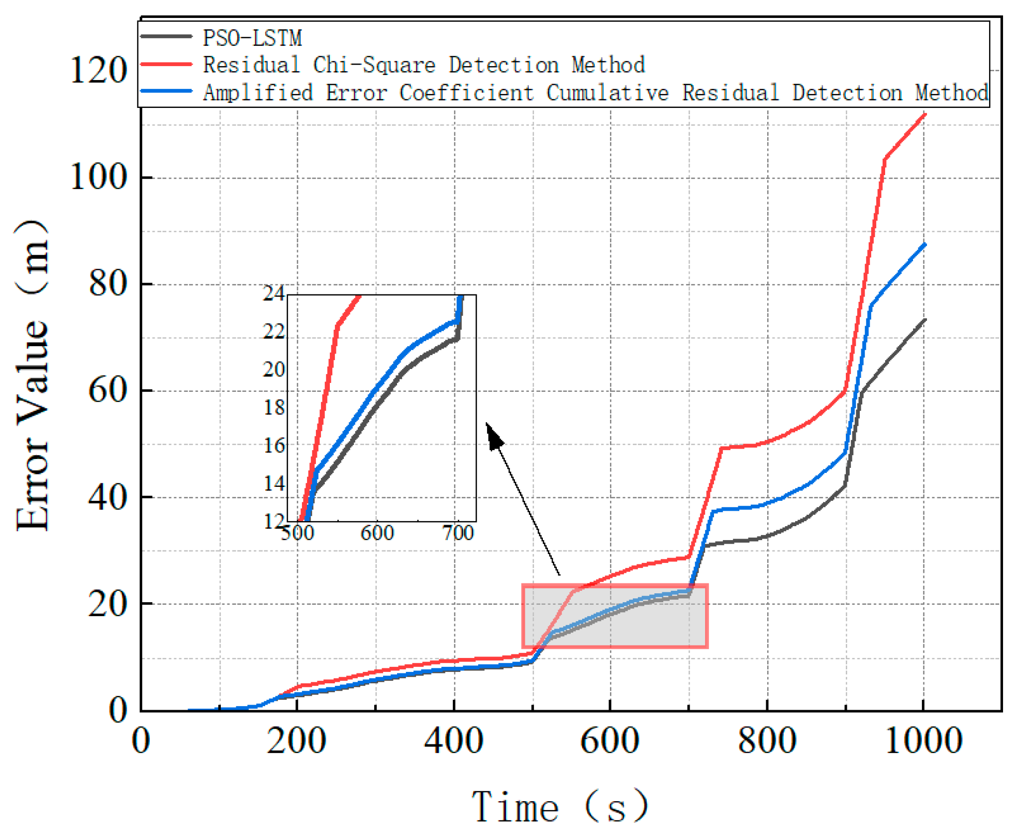
As shown in Figure 14, when an abrupt fault is introduced into the SINS/DVL integrated navigation system between 100 and 120 s, all three fault detection methods quickly isolate the fault and transition to the acoustic positioning system, thereby preventing the introduction of significant positional errors in the overall system. As subsequent gradual faults are added to the DVL data, the path deviation associated with the residual chi-square method increases over time, primarily due to its longer detection latency for gradual faults and its inability to promptly isolate the fault. In contrast, the error coefficient-amplified cumulative residual method and the PSO-LSTM fault detection method promptly detect gradual fault information, maintaining the stability of the positioning system. Additionally, compared to the error coefficient-amplified cumulative residual method, the PSO-LSTM fault detection method demonstrates a reduced positional error deviation. This is primarily because the PSO-LSTM method is trained on extensive data collected from the original sea area and constructs the fault detection function by calculating the difference between the new innovation from Kalman filtering and that predicted by the PSO-LSTM model. It does not require an accurate mathematical model of the system being monitored, which improves the adaptability of threshold settings and enhances fault detection performance. The above analysis demonstrates that, under the same application conditions, the trained PSO-LSTM fault detection method demonstrates superior detection performance for gradual faults.

6. Conclusions

This study examined the causes of faults in the AUV-integrated navigation system and categorized them into two distinct types based on numerical changes observed during fault occurrence: abrupt faults and gradual faults. In fault detection methods based on analytical models, a cumulative residual detection method with an error amplification coefficient has been proposed to address the limitations of the residual chi-square method in detecting gradual faults. This method utilizes the cumulative sum concept to formulate a non-parametric cumulative residual detection function, integrating an error amplification coefficient associated with fault frequency to enhance detection capability for gradual faults. The experimental results demonstrated that the error coefficient-amplified cumulative residual fault detection method outperforms the residual chi-square method regarding detection accuracy. To further improve detection capability for gradual faults, an artificial intelligence-based fault detection method was investigated. Specifically, a PSO-LSTM-based intelligent fault detection method was introduced. The integrated navigation system’s parameters, including velocity, angular velocity, specific force, and attitude angles, were derived from the fault-free system and served as input samples, while the Kalman filter innovations from the fault-free system were utilized as output samples for training the LSTM model. The PSO algorithm was employed to assist in determining the three hyperparameters of the LSTM model learning rate, number of hidden neurons, and iteration count, thereby preventing the LSTM model from converging to local optima during training. The predicted innovations from the PSO-LSTM model and the Kalman filter innovations of the integrated navigation system were subsequently compared to formulate a novel fault detection function. The experimental results revealed that the PSO-LSTM fault detection method exhibited superior sensitivity to gradual faults compared to both the residual chi-square and the error coefficient-amplified cumulative residual methods. Under expanded operational conditions for the AUV, the PSO-LSTM fault detection method is capable of promptly isolating faulty sensors, thereby mitigating their impact on the integrated navigation system and maintaining overall stability and reliability. However, the PSO-LSTM fault detection model relies on the training dataset. When the system encounters faults that are not present in the training data, these faults are difficult to detect, and the model demonstrates limited scalability.

The research on the fault detection algorithm in this paper is based on the assumption that the SINS is fault-free. In subsequent research, the superposition of faults of SINS gyroscopes, accelerometers, and other sensors can be further studied, and the effectiveness of the algorithm can be further verified through real-time sea trials.