
Understanding Wave Attenuation Across Marshes: Insights from Numerical Modeling

 , ,
, ,  , ,
, ,
Abstract
1. Introduction
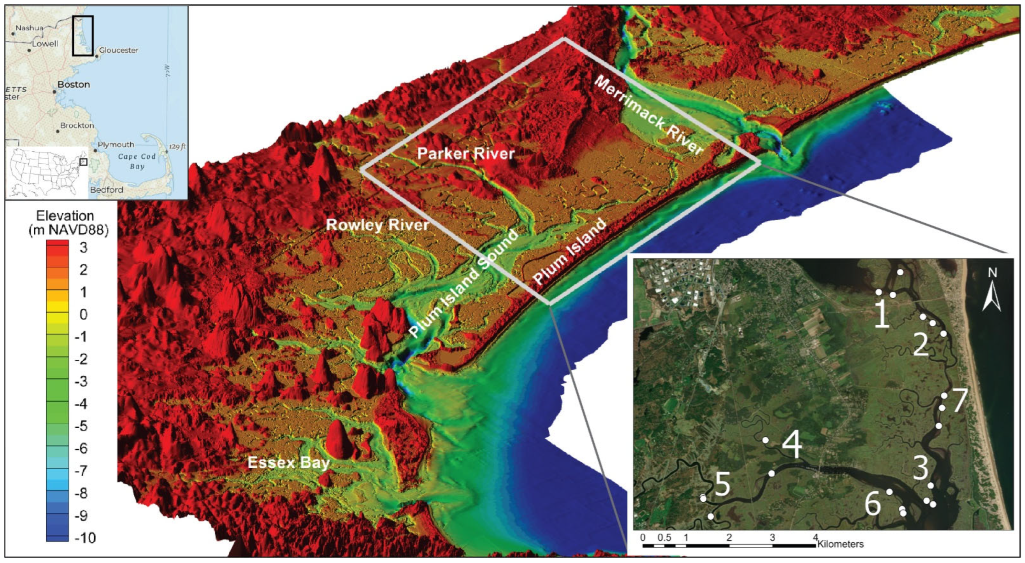
Physical Setting
2. Methods
2.1. Data, Observations, and Analysis
2.1.1. Bathymetry and Topography
2.1.2. Vegetation
2.2. Regional Hydrodynamic Modeling
2.2.1. Boundary Conditions
2.2.2. Calibration and Validation
2.2.3. Storm Characterization and Analysis
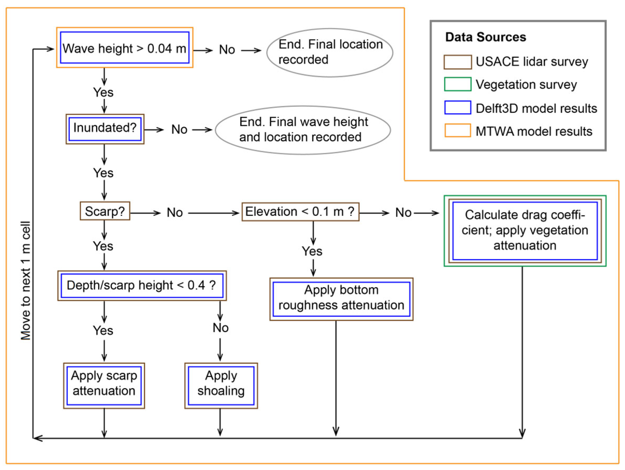
2.3. Marsh Transect Wave Attenuation Modeling
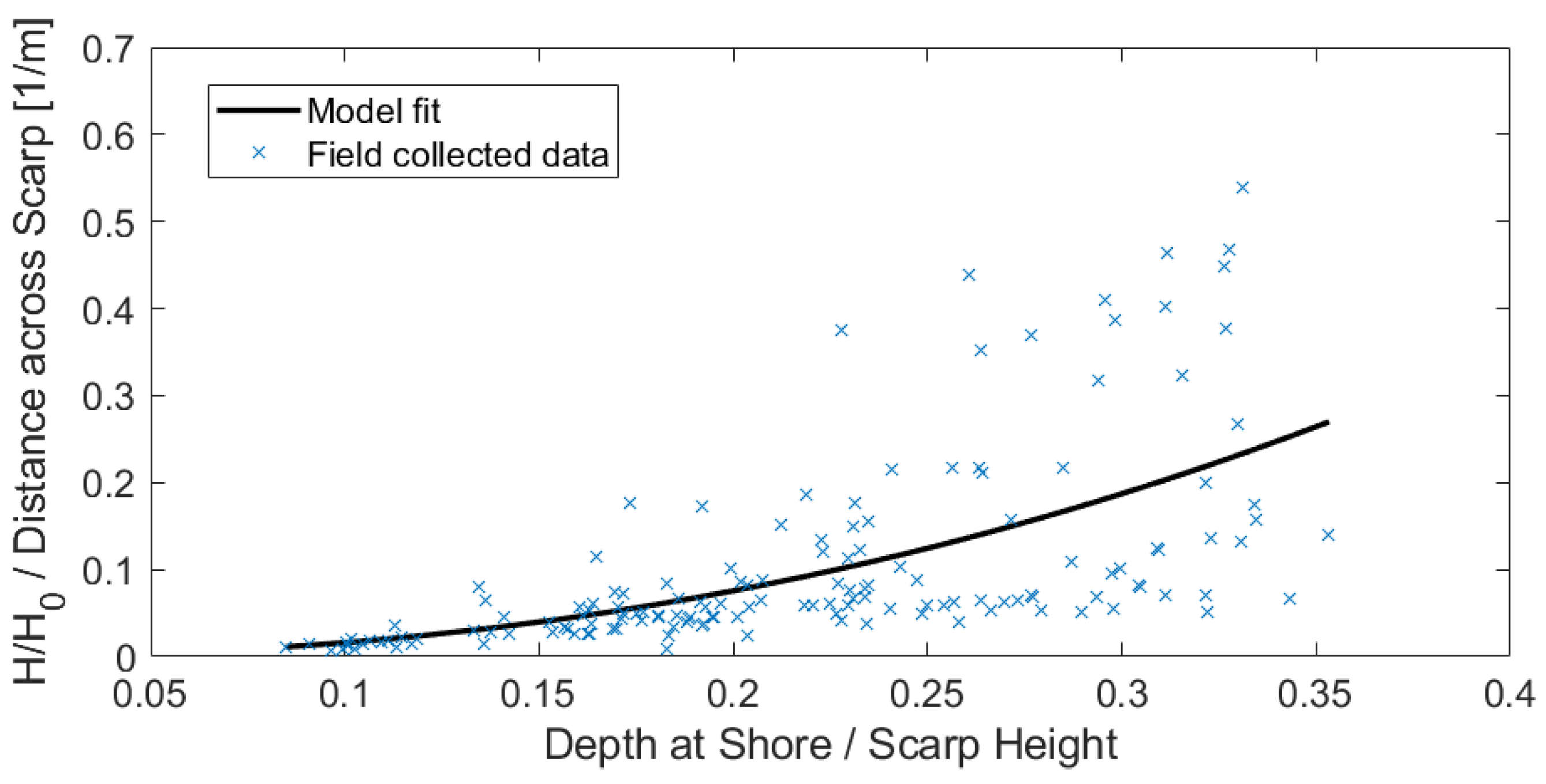
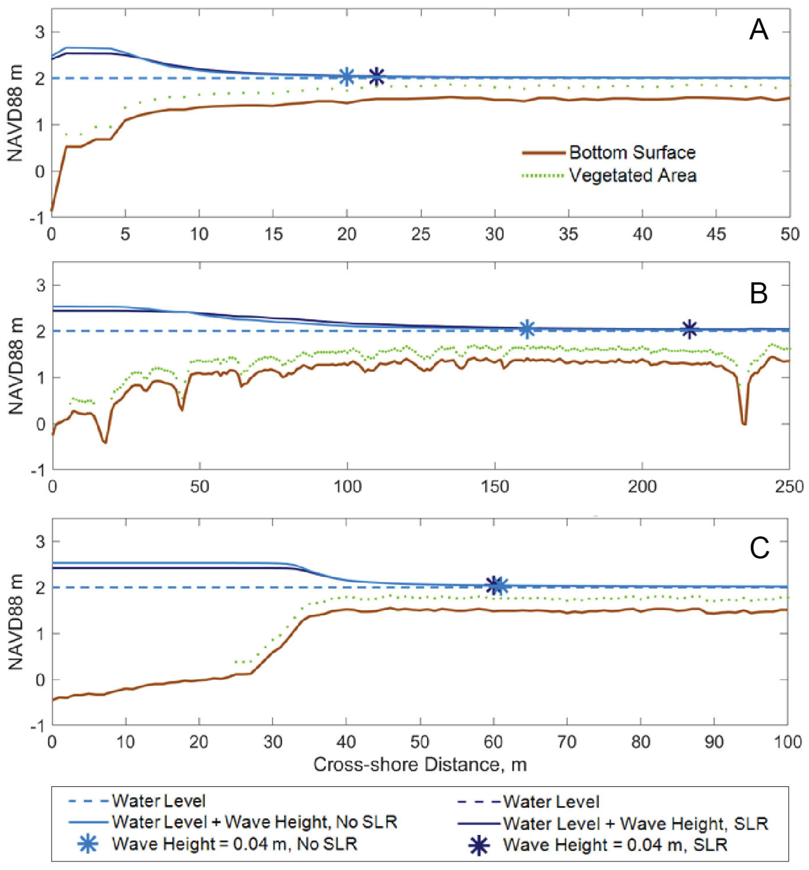
2.3.1. Interactions with Scarps and Shoaling
2.3.2. Bottom Roughness
2.3.3. Drag Due to Vegetation
2.4. Model Runs
2.4.1. Environmental Scenarios
2.4.2. Adjustment of Marsh Platform Due to Sea Level Rise
3. Results
3.1. Largest Wave Heights at the Marsh Edge
3.2. Wave Attenuation
3.2.1. Sea Level Rise
3.2.2. Vegetation Type
3.2.3. Conversion to Tidal Flat
3.2.4. Conversion to Tidal Flat with Lower Elevation
3.2.5. Lower Marsh Platform Elevation
3.2.6. Filling in Ditches
4. Discussion
4.1. Incident Wave Energy a Function of Tidal Regime and SLR
4.2. Effects of Vegetation
4.3. Shoreline Wave Heights Impacted by Loss of Elevation
4.4. Conservative Nature of Presented Modeling Approach
4.5. Wave Transformation over Scarped Edges Is Not Well Constrained
5. Conclusions
Supplementary Materials
Author Contributions
Funding
Data Availability Statement
Acknowledgments
Conflicts of Interest
References
- Shepard, C.C.; Crain, C.M.; Beck, M.W. The Protective Role of Coastal Marshes: A Systematic Review and Meta-Analysis. PLoS ONE 2011, 6, e27374. [Google Scholar] [CrossRef] [PubMed]
- Resio, D.T.; Westerink, J.J. Modeling the Physics of Storm Surges. Phys. Today 2008, 61, 33–38. [Google Scholar] [CrossRef]
- Mcowen, C.; Weatherdon, L.; Bochove, J.-W.; Sullivan, E.; Blyth, S.; Zockler, C.; Stanwell-Smith, D.; Kingston, N.; Martin, C.; Spalding, M.; et al. A Global Map of Saltmarshes. Biodivers. Data J. 2017, 5, e11764. [Google Scholar] [CrossRef]
- Petry, M.; Rogers, D. Nor’easter Slams into Greater Newburyport. The Daily News, 4 April 2024. [Google Scholar]
- Colle, B.A.; Zhang, Z.; Lombardo, K.A.; Chang, E.; Liu, P.; Zhang, M. Historical Evaluation and Future Prediction of Eastern North American and Western Atlantic Extratropical Cyclones in the CMIP5 Models during the Cool Season. J. Clim. 2013, 26, 6882–6903. [Google Scholar] [CrossRef]
- Zhang, Z.; Colle, B.A. Impact of Dynamically Downscaling Two CMIP5 Models on the Historical and Future Changes in Winter Extratropical Cyclones along the East Coast of North America. J. Clim. 2018, 31, 8499–8525. [Google Scholar] [CrossRef]
- FitzGerald, D.M.; Hughes, Z.J.; Georgiou, I.Y.; Black, S.; Novak, A. Enhanced, Climate-Driven Sedimentation on Salt Marshes. Geophys. Res. Lett. 2020, 47, e2019GL086737. [Google Scholar] [CrossRef]
- Leonardi, N.; Fagherazzi, S. How Waves Shape Salt Marshes. Geology 2014, 42, 887–890. [Google Scholar] [CrossRef]
- Leonardi, N.; Carnacina, I.; Donatelli, C.; Ganju, N.K.; Plater, A.J.; Schuerch, M.; Temmerman, S. Dynamic Interactions between Coastal Storms and Salt Marshes: A Review. Geomorphology 2018, 301, 92–107. [Google Scholar] [CrossRef]
- Houttuijn Bloemendaal, L.J.; FitzGerald, D.M.; Hughes, Z.J.; Novak, A.B.; Phippen, P. What Controls Marsh Edge Erosion? Geomorphology 2021, 386, 107745. [Google Scholar] [CrossRef]
- Bloemendaal, L.J.H.; FitzGerald, D.M.; Hughes, Z.J.; Novak, A.B.; Georgiou, I.Y. Reevaluating the Wave Power-Salt Marsh Retreat Relationship. Sci. Rep. 2023, 13, 2884. [Google Scholar] [CrossRef]
- Moeller, I.; Spencer, T.; French, J.R. Wind Wave Attenuation over Saltmarsh Surfaces: Preliminary Results from Norfolk, England. J. Coast. Res. 1996, 12, 1009–1016. [Google Scholar]
- Foster-Martinez, M.R.; Lacy, J.R.; Ferner, M.C.; Variano, E.A. Wave Attenuation across a Tidal Marsh in San Francisco Bay. Coast. Eng. 2018, 136, 26–40. [Google Scholar] [CrossRef]
- Feagin, R.A.; Innocenti, R.A.; Bond, H.; Wengrove, M.; Huff, T.P.; Lomonaco, P.; Tsai, B.; Puleo, J.; Pontiki, M.; Figlus, J.; et al. Does Vegetation Accelerate Coastal Dune Erosion during Extreme Events? Sci. Adv. 2023, 9, eadg7135. [Google Scholar] [CrossRef]
- NOAA National Oceanic and Atmospheric Administration. Available online: https://tidesandcurrents.noaa.gov/stationhome.html?id=8419870 (accessed on 1 June 2018).
- Vallino, J.J.; Hopkinson, C.S., Jr. Estimation of Dispersion and Characteristic Mixing Times in Plum Island Sound Estuary. Estuar. Coast. Shelf Sci. 1998, 46, 333–350. [Google Scholar] [CrossRef]
- Zhao, L.; Chen, C.; Vallino, J.; Hopkinson, C.; Beardsley, R.C.; Lin, H.; Lerczak, J. Wetland-estuarine-shelf Interactions in the Plum Island Sound and Merrimack River in the Massachusetts Coast. J. Geophys. Res. Ocean. 2010, 115, 2009JC006085. [Google Scholar] [CrossRef]
- Wilson, C.A.; Hughes, Z.J.; FitzGerald, D.M.; Hopkinson, C.S.; Valentine, V.; Kolker, A.S. Saltmarsh Pool and Tidal Creek Morphodynamics: Dynamic Equilibrium of Northern Latitude Saltmarshes? Geomorphology 2014, 213, 99–115. [Google Scholar] [CrossRef]
- Valentine, V.; Hopkinson, C., Jr. NCALM LIDAR: Plum Island, Massachusetts, USA: 18–19 April 2005. Elevation data and products produced by NSF-Supported National Center for Airborne Laser Mapping (NCALM) for Plum Island Ecosystems Long Term Ecological Research (PIE-LTER) Project. 2005. Available online: https://portal.edirepository.org/nis/metadataviewer?packageid=knb-lter-pie.422.1 (accessed on 1 June 2018).
- Millette, T.L.; Argow, B.A.; Marcano, E.; Hayward, C.; Hopkinson, C.S.; Valentine, V. Salt Marsh Geomorphological Analyses via Integration of Multitemporal Multispectral Remote Sensing with LIDAR and GIS. J. Coast. Res. 2010, 265, 809–816. [Google Scholar] [CrossRef]
- Chen, W.; Staneva, J.; Jacob, B.; Sánchez-Artús, X.; Wurpts, A. What-If Nature-Based Storm Buffers on Mitigating Coastal Erosion. Sci. Total Environ. 2024, 928, 172247. [Google Scholar] [CrossRef]
- Marino, M.; Nasca, S.; Alkharoubi, A.I.; Cavallaro, L.; Foti, E.; Musumeci, R.E. Efficacy of Nature-Based Solutions for Coastal Protection under a Changing Climate: A Modelling Approach. Coast. Eng. 2025, 198, 104700. [Google Scholar] [CrossRef]
- Cooperative Institute for Research in Environmental Sciences. Continuously Updated Digital Elevation Model (CUDEM)—1/9 Arc-Second Resolution Bathymetric-Topographic Tiles; Cooperative Institute for Research in Environmental Sciences: Boulder, CO, USA, 2014. [Google Scholar]
- OCM Partners 2014 USACE NAE Topobathy Lidar DEM: Newbury, MA, USA. Available online: https://www.fisheries.noaa.gov/inport/item/64731 (accessed on 1 June 2018).
- FitzGerald, D.M.; Hein, C.J.; Connell, J.E.; Hughes, Z.J.; Georgiou, I.Y.; Novak, A.B. Largest Marsh in New England near a Precipice. Geomorphology 2021, 379, 107625. [Google Scholar] [CrossRef]
- Shi, F.; Kirby, J.T.; Harris, J.C.; Geiman, J.D.; Grilli, S.T. A High-Order Adaptive Time-Stepping TVD Solver for Boussinesq Modeling of Breaking Waves and Coastal Inundation. Ocean. Model. 2012, 43–44, 36–51. [Google Scholar] [CrossRef]
- Shi, F.; Malej, M.; Smith, J.M.; Kirby, J.T. Breaking of Ship Bores in a Boussinesq-Type Ship-Wake Model. Coast. Eng. 2018, 132, 1–12. [Google Scholar] [CrossRef]
- Kirby, J.T. Chapter 1 Boussinesq Models and Applications to Nearshore Wave Propagation, Surf Zone Processes and Wave-Induced Currents. In Elsevier Oceanography Series; Elsevier: Amsterdam, The Netherlands, 2003; Volume 67, pp. 1–41. ISBN 978-0-444-51149-2. [Google Scholar]
- Collins, P.; MacMahan, J.; Thornton, E.; Benbow, C.; Jessen, P. Beach and Backward Bragg Sea-Swell Wave Reflection Across Rocky and Sandy Shores. J. Geophys. Res. Ocean. 2024, 129, e2023JC020177. [Google Scholar] [CrossRef]
- Xu, W.; Chen, C.; Htet, M.H.; Sarkar, M.S.I.; Tao, A.; Wang, Z.; Fan, J.; Jiang, D. Experimental Investigation on Bragg Resonant Reflection of Waves by Porous Submerged Breakwaters on a Horizontal Seabed. Water 2022, 14, 2682. [Google Scholar] [CrossRef]
- Gao, J.; Ma, X.; Dong, G.; Chen, H.; Liu, Q.; Zang, J. Investigation on the Effects of Bragg Reflection on Harbor Oscillations. Coast. Eng. 2021, 170, 103977. [Google Scholar] [CrossRef]
- Lesser, G.R.; Roelvink, J.A.; van Kester, J.A.T.M.; Stelling, G.S. Development and Validation of a Three-Dimensional Morphological Model. Coast. Eng. 2004, 51, 883–915. [Google Scholar] [CrossRef]
- Booij, N.; Ris, R.C.; Holthuijsen, L.H. A Third-generation Wave Model for Coastal Regions: 1. Model Description and Validation. J. Geophys. Res. Ocean. 1999, 104, 7649–7666. [Google Scholar] [CrossRef]
- Hanegan, K.C.; FitzGerald, D.M.; Georgiou, I.Y.; Hughes, Z.J. Long-Term Sea Level Rise Modeling of a Basin-Tidal Inlet System Reveals Sediment Sinks. Nat. Commun. 2023, 14, 7117. [Google Scholar] [CrossRef]
- Georgiou, I.Y.; Messina, F.; Sakib, M.M.; Zou, S.; Foster-Martinez, M.; Bregman, M.; Hein, C.J.; Fenster, M.S.; Shawler, J.L.; McPherran, K.; et al. Hydrodynamics and Sediment-Transport Pathways along a Mixed-Energy Spit-Inlet System: A Modeling Study at Chincoteague Inlet (Virginia, USA). J. Mar. Sci. Eng. 2023, 11, 1075. [Google Scholar] [CrossRef]
- Sullivan, J.C.; Torres, R.; Garrett, A.; Blanton, J.; Alexander, C.; Robinson, M.; Moore, T.; Amft, J.; Hayes, D. Complexity in Salt Marsh Circulation for a Semienclosed Basin. J. Geophys. Res. Earth Surf. 2015, 120, 1973–1989. [Google Scholar] [CrossRef]
- Liu, K.; Chen, Q.; Hu, K.; Xu, K.; Twilley, R.R. Modeling Hurricane-Induced Wetland-Bay and Bay-Shelf Sediment Fluxes. Coast. Eng. 2018, 135, 77–90. [Google Scholar] [CrossRef]
- Caldwell, R.L.; Edmonds, D.A. The Effects of Sediment Properties on Deltaic Processes and Morphologies: A Numerical Modeling Study. J. Geophys. Res. Earth Surf. 2014, 119, 961–982. [Google Scholar] [CrossRef]
- Mukai, A.Y.; Westerink, J.J.; Luettich, R.A. Guidelines for Using Eastcoast 2001 Database of Tidal Constituents Within Western North Atlantic Ocean, Gulf of Mexico and Caribbean Sea; US Army Engineer Research and Development Center, Coastal and Hydraulics Laboratory: Vicksburg, MS, USA, 2002. [Google Scholar]
- Cialone, M.A.; Bocamazo, L.M.; Nadal-Caraballo, N.C.; Massey, T.C.; Melby, J.A. North Atlantic Coast Comprehensive Study (Naccs) Storm Simulation and Statistical Analysis: Part I–Overview. In The Proceedings of the Coastal Sediments 2015; World Scientific: San Diego, CA, USA, 2015. [Google Scholar]
- USACE (US Army Corps of Engineers). Wave Information Study (WIS); USACE: Wiesbaden, Germany, 2023. [Google Scholar]
- Foster-Martinez, M.R.; Alizad, K.; Hagen, S.C. Estimating Wave Attenuation at the Coastal Land Margin with a GIS Toolbox. Environ. Model. Softw. 2020, 104788. [Google Scholar] [CrossRef]
- Hijuelos, A.C.; Dijkstra, J.T.; Carruthers, T.J.B.; Heynert, K.; Reed, D.J.; van Wesenbeeck, B.K. Linking Management Planning for Coastal Wetlands to Potential Future Wave Attenuation under a Range of Relative Sea-Level Rise Scenarios. PLoS ONE 2019, 14, e0216695. [Google Scholar] [CrossRef]
- Dean, R.G.; Dalrymple, R.A. Water Wave Mechanics for Engineers and Scientists; World Scientific Publishing Co., Inc.: Singapore, 1991; Volume 2. [Google Scholar]
- Nielsen, P. Coastal Bottom Boundary Layers and Sediment Transport; World Scientific Publishing Co., Inc.: Singapore, 1992; Volume 4. [Google Scholar]
- Kopp, R.E.; Kemp, A.C.; Bittermann, K.; Horton, B.P.; Donnelly, J.P.; Gehrels, W.R.; Hay, C.C.; Mitrovica, J.X.; Morrow, E.D.; Rahmstorf, S. Temperature-Driven Global Sea-Level Variability in the Common Era. Proc. Natl. Acad. Sci. USA. 2016, 113, E1434–E1441. [Google Scholar] [CrossRef]
- Donnelly, J.P.; Bertness, M.D. Rapid Shoreward Encroachment of Salt Marsh Cordgrass in Response to Accelerated Sea-Level Rise. Proc. Natl. Acad. Sci. 2001, 98, 14218–14223. [Google Scholar] [CrossRef]
- Maza, M.; Lara, J.L.; Losada, I.J. Experimental Analysis of Wave Attenuation and Drag Forces in a Realistic Fringe Rhizophora Mangrove Forest. Adv. Water Resour. 2019, 131, 103376. [Google Scholar] [CrossRef]
- Augustin, L.N.; Irish, J.L.; Lynett, P. Laboratory and Numerical Studies of Wave Damping by Emergent and Near-Emergent Wetland Vegetation. Coast. Eng. 2009, 56, 332–340. [Google Scholar] [CrossRef]
- Anderson, M.E.; Smith, J.M. Wave Attenuation by Flexible, Idealized Salt Marsh Vegetation. Coast. Eng. 2014, 83, 82–92. [Google Scholar] [CrossRef]
- Blackmar, P.J.; Cox, D.T.; Wu, W.-C. Laboratory Observations and Numerical Simulations of Wave Height Attenuation in Heterogeneous Vegetation. J. Waterw. Port Coast. Ocean. Eng. 2014, 140, 56–65. [Google Scholar] [CrossRef]
- Rupprecht, F.; Möller, I.; Paul, M.; Kudella, M.; Spencer, T.; van Wesenbeeck, B.K.; Wolters, G.; Jensen, K.; Bouma, T.J.; Miranda-Lange, M.; et al. Vegetation-Wave Interactions in Salt Marshes under Storm Surge Conditions. Ecol. Eng. 2017, 100, 301–315. [Google Scholar] [CrossRef]
- Ozeren, Y.; Wren, D.G.; Wu, W. Experimental Investigation of Wave Attenuation through Model and Live Vegetation. J. Waterw. Port Coast. Ocean Eng. 2014, 140, 04014019. [Google Scholar] [CrossRef]
- Paul, K.I.; Roxburgh, S.H.; Chave, J.; England, J.R.; Zerihun, A.; Specht, A.; Lewis, T.; Bennett, L.T.; Baker, T.G.; Adams, M.A.; et al. Testing the Generality of Above-ground Biomass Allometry across Plant Functional Types at the Continent Scale. Glob. Change Biol. 2016, 22, 2106–2124. [Google Scholar] [CrossRef]
- Van Veelen, T.J.; Fairchild, T.P.; Reeve, D.E.; Karunarathna, H. Experimental Study on Vegetation Flexibility as Control Parameter for Wave Damping and Velocity Structure. Coast. Eng. 2020, 157, 103648. [Google Scholar] [CrossRef]
- Cassalho, F.; De Lima, A.D.S.; Coleman, D.J.; Henke, M.; Miesse, T.W.; Coelho, G.D.A.; Ferreira, C.M. Projecting Future Wave Attenuation by Vegetation from Native and Invasive Saltmarsh Species in the United States. Reg. Stud. Mar. Sci. 2023, 68, 103264. [Google Scholar] [CrossRef]
- Lara, J.L.; Maza, M.; Ondiviela, B.; Trinogga, J.; Losada, I.J.; Bouma, T.J.; Gordejuela, N. Large-Scale 3-D Experiments of Wave and Current Interaction with Real Vegetation. Part 1: Guidelines for Physical Modeling. Coast. Eng. 2016, 107, 70–83. [Google Scholar] [CrossRef]
- Maza, M.; Lara, J.L.; Losada, I.J. Tsunami Wave Interaction with Mangrove Forests: A 3-D Numerical Approach. Coast. Eng. 2015, 98, 33–54. [Google Scholar] [CrossRef]
- Möller, I.; Kudella, M.; Rupprecht, F.; Spencer, T.; Paul, M.; van Wesenbeeck, B.K.; Wolters, G.; Jensen, K.; Bouma, T.J.; Miranda-Lange, M.; et al. Wave Attenuation over Coastal Salt Marshes under Storm Surge Conditions. Nat. Geosci 2014, 7, 727–731. [Google Scholar] [CrossRef]
- Paul, M.; Kerpen, N.B. Erosion Protection by Winter State of Salt Marsh Vegetation. J. Ecohydraul. 2022, 7, 144–153. [Google Scholar] [CrossRef]
- Poppema, D.W.; Willemsen, P.W.; de Vries, M.B.; Zhu, Z.; Borsje, B.W.; Hulscher, S.J. Experiment-Supported Modelling of Salt Marsh Establishment. Ocean. Coast. Manag. 2019, 168, 238–250. [Google Scholar] [CrossRef]
- Knutson, P.L.; Brochu, R.A.; Seelig, W.N.; Inskeep, M. Wave Damping in Spartina alterniflora Marshes. Wetlands 1982, 2, 87–104. [Google Scholar] [CrossRef]
- Jadhav, R.S.; Chen, Q. Field Investigation of Wave Dissipation over Salt Marsh Vegetation During Tropical Cyclone. Int. Conf. Coastal. Eng. 2012, 1, 41. [Google Scholar] [CrossRef]
- Paquier, A.-E.; Haddad, J.; Lawler, S.; Ferreira, C.M. Quantification of the Attenuation of Storm Surge Components by a Coastal Wetland of the US Mid Atlantic. Estuaries Coasts 2016, 40, 930–946. [Google Scholar] [CrossRef]
- Wu, W.; Ozeren, Y.; Wren, D.; Chen, Q.; Zhang, G.; Holland, M.; Ding, Y.; Kuiry, S.; Zhang, M.; Jadhav, R.; et al. SERRI Project: Investigations of Surge and Wave Reduction by Vegetation; SERRI Report 80037-01; National Center for Computational Hydroscience and Engineering, University of Mississippi: Oxford, MS, USA, 2011. [Google Scholar]
- Park, R.A.; Armentano, T.V.; Cloonan, C.L. Predicting the Effects of Sea Level Rise on Coastal Wetlands. Eff. Changes Stratos. Ozone Glob. Clim. 1986, 4, 129–152. [Google Scholar]
- Clough, J.; Park, R.A.; Fuller, R. SLAMM 6 Beta Technical Documentation; Warren Pinnacle: Waitsfield, VT, USA, 2010; p. 49. [Google Scholar]
- Bolle, A.; Mercelis, P.; Roelvink, D.; Haerens, P.; Trouw, K. Application and Validation of XBeach for Three Different Field Sites. Coast. Eng. Proc. 2011, 1, 40. [Google Scholar] [CrossRef]
- Harley, M.; Armaroli, C.; Ciavola, P. Evaluation of XBeach Predictions for a Real-Time Warning System in Emilia-Romagna, Northern Italy. J. Coast. Res. 2011, 1861–1865. Available online: https://www.jstor.org/stable/26482499 (accessed on 25 April 2025).
- van Rooijen, A.A.; van Thiel de Vries, J.S.M.; McCall, R.T.; van Dongeren, A.R.; Roelvink, J.A.; Reniers, A.J.H.M. Modeling of Wave Attenuation by Vegetation with XBeach. In Proceedings of the E-Proceedings of the 36th IAHR World Congress, The Hague, The Netherlands, 28 June–3 July 2015; IAHR: Madrid, Spain, 2015; Volume 2016, p. 6. [Google Scholar]
- Taylor-Burns, R.; Nederhoff, K.; Lacy, J.R.; Barnard, P.L. The Influence of Vegetated Marshes on Wave Transformation in Sheltered Estuaries. Coast. Eng. 2023, 184, 104346. [Google Scholar] [CrossRef]
- de Ridder, M.P.; Smit, P.B.; van Dongeren, A.R.; McCall, R.T.; Nederhoff, K.; Reniers, A.J. Efficient Two-Layer Non-Hydrostatic Wave Model with Accurate Dispersive Behaviour. Coast. Eng. 2021, 164, 103808. [Google Scholar] [CrossRef]
- Van Rooijen, A.; McCall, R.; Van Thiel de Vries, J.; Van Dongeren, A.; Reniers, A.; Roelvink, J. Modeling the Effect of Wave-Vegetation Interaction on Wave Setup. J. Geophys. Res. Ocean. 2016, 121, 4341–4359. [Google Scholar] [CrossRef]
- Alizad, K.; Hagen, S.C.; Morris, J.T.; Bacopoulos, P.; Bilskie, M.V.; Weishampel, J.F.; Medeiros, S.C. A Coupled, Two-Dimensional Hydrodynamic-Marsh Model with Biological Feedback. Ecol. Model. 2016, 327, 29–43. [Google Scholar] [CrossRef]
- Alizad, K.; Hagen, S.C.; Medeiros, S.C.; Bilskie, M.V.; Morris, J.T.; Balthis, L.; Buckel, C.A. Dynamic Responses and Implications to Coastal Wetlands and the Surrounding Regions under Sea Level Rise. PLoS ONE 2018, 13, e0205176. [Google Scholar] [CrossRef] [PubMed]
- Garzon, J.L.; Maza, M.; Ferreira, C.M.; Lara, J.L.; Losada, I.J. Wave Attenuation by Spartina Saltmarshes in the Chesapeake Bay under Storm Surge Conditions. J. Geophys. Res. Ocean. 2019, 124, 5220–5243. [Google Scholar] [CrossRef]
- Wiberg, P.L.; Sherwood, C.R. Calculating Wave-Generated Bottom Orbital Velocities from Surface-Wave Parameters. Comput. Geosci. 2008, 34, 1243–1262. [Google Scholar] [CrossRef]
- Kobayashi, N.; Raichle, A.W.; Asano, T. Wave Attenuation by Vegetation. J. Waterw. Port Coast. Ocean Eng. 1993, 119, 30–48. [Google Scholar] [CrossRef]
- Mendez, F.J.; Losada, I.J. An Empirical Model to Estimate the Propagation of Random Breaking and Nonbreaking Waves over Vegetation Fields. Coast. Eng. 2004, 51, 103–118. [Google Scholar] [CrossRef]
- Foster-Martinez, M.; FitzGerald, D.; Georgiou, I.; Hughes, Z. Assessing Storm Energy Reduction by the Vegetated Salt Marsh Platform in Newbury, MA, Pressure Timeseries. Zenodo 2025. [Google Scholar] [CrossRef]
- Foster-Martinez, M.; Georgiou, I. Marsh Transect Wave Attenuation (MTWA) Model. Zenodo 2025. [Google Scholar] [CrossRef]


| Event | Date | Time (UTC) | (m) | (s) | * |
|---|---|---|---|---|---|
| 4 | 16 January 1980 | 12:00 | 6.37 | 12.79 | 80.0 |
| 5 | 14 March 2010 | 15:00 | 6.11 | 12.08 | 99.0 |
| 6 | 12 December 1992 | 08:00 | 6.08 | 12.77 | 93.0 |
| 7 | 9 February 2013 | 03:00 | 5.86 | 10.81 | 61.0 |
| Scenario | Parameters Used and/or Altered |
|---|---|
| 1. Base | Average vegetation characteristics; unaltered DEM |
| 2. All Spartina alterniflora | Spartina alterniflora characteristics; unaltered DEM |
| 3. All Spartina patens | Spartina patens characteristics; unaltered DEM |
| 4. Tidal flat | Vegetation drag switched off; unaltered DEM |
| 5. Tidal flat, lower elevation | Vegetation drag switched off; DEM lowered |
| 6. Lower elevation | Average vegetation characteristics; DEM lowered |
| 7. Ditches filled | Average vegetation characteristics; elevation of ditches increased |
Disclaimer/Publisher’s Note: The statements, opinions and data contained in all publications are solely those of the individual author(s) and contributor(s) and not of MDPI and/or the editor(s). MDPI and/or the editor(s) disclaim responsibility for any injury to people or property resulting from any ideas, methods, instructions or products referred to in the content. |
© 2025 by the authors. Licensee MDPI, Basel, Switzerland. This article is an open access article distributed under the terms and conditions of the Creative Commons Attribution (CC BY) license (https://creativecommons.org/licenses/by/4.0/).
Share and Cite
Foster-Martinez, M.R.; Georgiou, I.Y.; FitzGerald, D.M.; Hughes, Z.J.; Novak, A.; Sakib, M.M. Understanding Wave Attenuation Across Marshes: Insights from Numerical Modeling. J. Mar. Sci. Eng. 2025, 13, 1188. https://doi.org/10.3390/jmse13061188
Foster-Martinez MR, Georgiou IY, FitzGerald DM, Hughes ZJ, Novak A, Sakib MM. Understanding Wave Attenuation Across Marshes: Insights from Numerical Modeling. Journal of Marine Science and Engineering. 2025; 13(6):1188. https://doi.org/10.3390/jmse13061188
Chicago/Turabian StyleFoster-Martinez, Madeline R., Ioannis Y. Georgiou, Duncan M. FitzGerald, Zoe J. Hughes, Alyssa Novak, and Md Mohiuddin Sakib. 2025. "Understanding Wave Attenuation Across Marshes: Insights from Numerical Modeling" Journal of Marine Science and Engineering 13, no. 6: 1188. https://doi.org/10.3390/jmse13061188
APA StyleFoster-Martinez, M. R., Georgiou, I. Y., FitzGerald, D. M., Hughes, Z. J., Novak, A., & Sakib, M. M. (2025). Understanding Wave Attenuation Across Marshes: Insights from Numerical Modeling. Journal of Marine Science and Engineering, 13(6), 1188. https://doi.org/10.3390/jmse13061188