Hydrodynamic Calculation and Analysis of a Complex-Shaped ROV Moving near the Wall Based on CFDs

Abstract

Remotely operated vehicles (ROVs) face challenges in maneuvering and rapidly detecting and repairing large offshore platforms. The accurate research on the hydrodynamics of the ROV, which moves close to the wall, is of great significance for its maneuverability. This study uses computational fluid dynamics (CFDs) to analyze the hydrodynamic characteristics of an ROV when it is moving near the wall, considering factors such as structural asymmetry, speed, and distance from the wall. This study applies multiple linear regression to extract relevant hydrodynamic coefficients and develops a mathematical model that simulates the impact of these factors on ROV performance. The results indicate that the wall’s influence on hydrodynamic forces is significant. Total resistance increases as the ROV moves closer to the wall, and the effect becomes more pronounced at higher speeds. Pressure differential resistance is the dominant factor affecting ROV performance, while viscous resistance remains low and is mostly unaffected by wall proximity. These findings provide valuable insights into calculating hydrodynamic coefficients and modeling the dynamics of ROVs with complex shapes operating near the wall.

1. Introduction

With the widespread application of remotely operated vehicles (ROVs) in fields such as deep-sea exploration [1], oil platform maintenance [2], and subsea pipeline inspection [3], their hydrodynamic performance in near-wall environments has become a critical factor influencing their maneuverability and operational efficiency [4,5]. When ROVs approach such surfaces, significant changes occur in the surrounding flow characteristics. These changes can profoundly affect several aspects of ROV operation, including control performance, energy efficiency, and overall stability. For instance, boundary layer effects become more pronounced, leading to increased pressure drag and variations in viscous drag. Such phenomena not only complicate the control algorithms required for precise navigation but also increase the energy demand placed on the vehicle’s propulsion systems. Consequently, conducting in-depth studies into the hydrodynamic characteristics of ROVs during near-wall motion and developing accurate dynamic models are of great practical significance. These efforts contribute directly to improving the design, manipulation, and control of ROVs, ultimately enhancing their effectiveness in challenging underwater environments.

In recent years, the swift advancement of computational fluid dynamics (CFDs) technology has enabled researchers to more precisely simulate and analyze the hydrodynamic performance of ROVs, thereby estimating hydrodynamic coefficients. Valencia et al. [6] used CFDs tools to model and simulate an ROV aimed at surveillance and inspection tasks within port facilities, emphasizing the importance of reliable visual information and the role of CFDs in achieving this goal. Building upon this foundation, Ramírez-Macías et al. [7] focused on hydrodynamic modeling of an inspection-class ROV, employing a viscous-flow solver to accurately predict maneuvering coefficients essential for control, and highlighted the importance of detailed geometric modeling and viscous flow analysis in capturing the ROV’s hydrodynamic performance. Katsui et al. [8] investigated the flow around a crawler-driven ROV on the seafloor, using CFDs to evaluate hydrodynamic forces and better understand the vehicle’s interaction with its environment. Baital et al. [9] investigated pressure and drag forces on a low-cost mini ROV, providing valuable data for hardware and material selection. The CFDs method, through numerical simulations of fluid–object interactions, has provided a powerful tool for the hydrodynamic analysis of ROVs. Particularly, the motion of ROVs near walls or the seafloor involves complex fluid dynamics phenomena such as boundary layer effects, pressure drag, and variations in viscous drag. Investigating these phenomena facilitates the optimization of ROV structural design and enhances their maneuverability.

In research on the hydrodynamics of ROVs moving near walls, a significant amount of the literature has explored the fluid dynamics of underwater robots under various conditions, indicating that the hydrodynamic performance is highly sensitive to boundary effects [10,11]. Du et al. [12] used CFDs simulations to study unmanned underwater vehicles (UUVs) approaching the seafloor, finding that both the seafloor distance and attack angle significantly affect drag, lift, and pitch moment, with attraction forces increasing as distance decreases, highlighting the importance of precise control mechanisms to counteract these effects. Mitra et al. [13] conducted both experimental and numerical studies on the hydrodynamic characteristics of autonomous underwater vehicles (AUVs) in complex seabed topographies, showing that seafloor slope and fluid conditions significantly impact performance, especially in narrow channels and complex terrains. Li et al. [14] proposed a new hydrodynamic model to analyze the hydrodynamic behavior of ROVs near walls, showing that wall effects significantly altered the total drag, with drag and pitch moment increasing as the proximity to the wall decreased. Liu et al. [15] further explored the hydrodynamic performance of UUVs moving near the seafloor and proposed computational models related to seabed distance and Reynolds number. Wu et al. [16] used CFDs methods to study the hydrodynamics of the DARPA SUBOFF model near a level bottom. They found that drag increased nonlinearly as cruising altitude decreased due to changes in pressure and viscous effects. The study also explored how Reynolds number and attack angle affected flow patterns and drag characteristics. Validation against experimental data confirmed the accuracy of their findings. This work provides valuable insights for designing efficient underwater vehicle systems. In summary, the above studies demonstrate that the boundary effects exerted by the wall significantly influence the hydrodynamic performance of underwater vehicles, such as drag, lift, moment changes, and flow pattern variations, emphasizing the importance of boundary conditions in near-wall movement.

Existing research has revealed the complexity and diversity of the hydrodynamic characteristics of ROVs and other underwater robots in near-wall motion, with CFDs methods providing strong support for such studies. However, a significant challenge remains: ROVs are typically more asymmetric and complex in structure compared to typical streamlined structures, which makes their hydrodynamic behavior more complicated. That is, the impact of structural asymmetry on hydrodynamics needs to be discussed. For instance, Xu et al. [17] conducted experimental analyses on the hydrodynamic behavior of a novel asymmetric-shaped ROV. Their study revealed unique flow patterns and interactions that arise due to the vehicle’s unconventional geometry. These findings underscore the importance of considering asymmetry in the design phase to optimize performance and stability. Similarly, Zhang et al. [18] explored the relationship between structural asymmetry and pressure resistance, demonstrating that the asymmetrical designs of ROVs lead to a notable difference in pressure resistance during forward versus backward sailing, as well as ascending and descending movements and this difference becomes substantially more pronounced with an increase in velocity. Zan et al. [19] employed a combination of experiments and numerical simulations to conduct a comprehensive analysis of the ROV’s movements in different directions. The study revealed that the asymmetric design of the ROV had a significant and differentiated impact on the forces and torques it experienced during longitudinal, vertical, and oblique movements. This means that the flow field around the vehicle becomes uneven, resulting in unbalanced forces such as drag and lift. Such imbalances can compromise the vehicle’s stability and control, especially in dynamic environments where precise navigation is essential. By addressing these challenges, researchers and engineers can develop more robust hydrodynamic models and improve the overall performance of ROVs in near-wall operations.

Although several studies have investigated various factors affecting the hydrodynamics of ROVs, the majority have not thoroughly examined the performance of asymmetrical ROV shapes in dynamic near-wall environments. This gap in research is significant, as the behavior of ROVs in such environments can differ substantially from their performance in open water. For instance, when an ROV operates close to a wall or seabed, the interaction between the vehicle and the boundary layer can lead to complex flow patterns. These interactions may result in increased drag, altered lift forces, and changes in stability, all of which can impact the vehicle’s maneuverability and energy efficiency. Moreover, the near-wall hydrodynamics of ROVs have not been quantified in detail, leaving uncertainties in predicting how these vehicles will behave in confined spaces. Without precise quantification, it becomes challenging for engineers to design ROVs that can operate effectively in environments where walls or other structures are present.

In view of this, the current research seeks to employ CFDs methods to systematically investigate the hydrodynamic characteristics of complex-shaped ROVs during near-wall motion. Particular attention is given to how structural asymmetry, cruising velocity, and proximity to the wall influence hydrodynamic performance. By establishing hydrodynamic mathematical models adapted to near-wall environments, this study will comprehensively analyze the flow field characteristics under various conditions and their interactions with the wall. These findings are expected to contribute novel insights and robust methodologies for advancing hydrodynamic model formulation and improving the accuracy of hydrodynamic calculations.

2. Structure and Hydrodynamic Model of ROV

2.1. Structure

The research object in this paper is an open-frame ROV equipped with a mechanical arm, a brush, and an observation device. This ROV is designed for damage detection, repair, and routine inspections of large marine structures, with a designed water depth of 500 m. Its frame size is 1.8 m × 1.8 m × 1.07 m (length × width × height), and its weight is 904.9 kg. The ROV is equipped with a sophisticated propulsion system consisting of eight thrusters, which are strategically arranged to provide comprehensive control over the vehicle’s movement. Specifically, there are four horizontal thrusters and four vertical thrusters. This specific configuration of thrusters on the ROV allows it to achieve highly precise maneuverability across all six degrees of freedom, which is essential for effective underwater operations. The six degrees of freedom include pitch, roll, yaw, sway, heave, and surge. These thrusters exhibit significant cross-coupling.

The ROV features a removable track mechanism, which can be adjusted to suit various structural and seabed surfaces in different working environments and can be installed or removed according to sea conditions and weight requirements. The buoyancy material is installed on the top of the body, but the metacentric height needs to be noted to ensure that the device can roll under the action of the recovery moment. The 3D model of the ROV is presented in Figure 1a.

2.2. Hydrodynamic Model

For a clearer description of the ROV’s motion, two coordinate systems are defined [20]: a fixed coordinate system E-x₀y₀z₀ and a moving coordinate system G-x_by_bz_b, as illustrated in Figure 1b. The origin of the fixed system is located at any point on Earth. This system serves as a global reference frame that allows us to track the absolute position and orientation of the ROV in relation to the surrounding environment. The origin of the moving system aligns with the ROV’s center of mass. This system provides a local perspective, enabling detailed analysis of the vehicle’s motion relative to its own body.

In the fixed coordinate system, the ROV’s position and orientation are denoted by the vector: η = [x y z ϕ θ ψ]^T.

Within the moving coordinate system, velocity is represented by the vector: V = [u v w p q r]^T, while the forces and moments acting on the ROV are described by the vector: F = [X Y Z K M N]^T.

Detailed definitions of the motion under various degrees of freedom are provided in

Table 1. The notation of ROV motion.

Degree of Freedom	Positions and Euler Angles	Linear and Angular Velocity	Forces and Moments
1 (Surge)	x (m)	u (m/s)	X (N)
2 (Sway)	y (m)	v (m/s)	Y (N)
3 (Heave)	z (m)	w (m/s)	Z (N)
4 (Roll)	ϕ (rad)	p (rad/s)	K (N·m)
5 (Pitch)	θ (rad)	q (rad/s)	M (N·m)
6 (Yaw)	ψ (rad)	r (rad/s)	N (N·m)

. This table serves as a valuable reference, offering precise descriptions of each parameter and its significance in the overall kinematic and dynamic model of the ROV. By utilizing these coordinate systems and associated vectors, researchers and engineers can achieve a clearer and more accurate description of the ROV’s complex motion patterns in underwater environments.

By using the transformation of the kinematics matrix, which links the vehicle’s velocity in the moving coordinate system to its position in the fixed coordinate system, the equation of motion can be expressed as follows [21]:

$$\left(\begin{array}{c}\dot{x}\\ \dot{y}\\ \dot{z}\end{array}\right)=\left(\begin{array}{ccc}\cos \theta \cos \psi & \sin \varphi \sin \theta \cos \psi -\cos \varphi \sin \psi & \cos \varphi \sin \theta \cos \psi +\sin \varphi \sin \psi \\ \cos \theta \sin \psi & \sin \varphi \sin \theta \sin \psi +\cos \varphi \cos \psi & \cos \varphi \sin \theta \sin \psi -\sin \varphi \cos \psi \\ -\sin \theta & \sin \varphi \cos \theta & \cos \varphi \cos \theta \end{array}\right)\left(\begin{array}{c}u\\ v\\ w\end{array}\right)$$

(1)

$$\left(\begin{array}{c}\dot{\varphi }\\ \dot{\theta }\\ \dot{\psi }\end{array}\right)=\left(\begin{array}{ccc}1& \sin \varphi \tan \theta & \cos \varphi \tan \theta \\ 0& \cos \varphi & -\sin \varphi \\ 0& \sin \varphi \sec \theta & \cos \varphi \sec \theta \end{array}\right)\left(\begin{array}{c}\mathit{p}\\ q\\ r\end{array}\right)$$

(2)

In order to simplify the motion equation and better analyze the dynamic behavior of a remotely operated vehicle (ROV), the origin of the moving coordinate system is strategically placed at the ROV’s center of gravity. This selection guarantees that the three coordinate axes are approximately oriented along the principal inertia axes, thereby reducing coupling effects among various degrees of freedom. Such alignment simplifies the mathematical representation of rotational and translational motions by reducing unnecessary cross terms in the equations.

By applying Newton’s second laws and Euler’s rotational equations, the resulting six-degrees-of-freedom dynamic equation for the ROV can be derived as follows:

$$M_{\mathrm{RB}}\dot{V}+C_{\mathrm{RB}}\left(V\right)V=F$$

(3)

where M_RB represents the mass matrix of the ROV, which encapsulates the inertial properties of the vehicle in terms of its mass distribution and C_RB denotes the Coriolis and centripetal force matrix, which depends on the ROV’s velocity components. These forces arise due to the relative motion of the ROV within its own coordinate frame and play a critical role in accurately modeling the nonlinear dynamics of the system. Additionally, F = [X Y Z K M N]^T represents the total external force (moment) acting on the ROV.

Through expanding this model, the force and moment equations can be expressed explicitly in terms of their respective components. By transforming these equations into the fixed coordinate system, the complete dynamic equations of the ROV can be obtained as follows:

$$\begin{array}{l}m\cdot (\dot{u}-vr+wq)=X\\ m\cdot (\dot{v}-wp+ur)=Y\\ m\cdot (\dot{w}-uq+vp)=Z\\ I_x\dot{p}+(I_z-I_y)qr=K\\ I_y\dot{q}+(I_x-I_z)rp=M\\ I_z\dot{r}+(I_y-I_x)pq=N\end{array}$$

(4)

where m represents the mass of the ROV; X, Y, Z, K, M, and N indicate external forces and moments acting on the ROV; and I_x, I_y and I_z refer to the mass moment of inertia of the ROV about its three principal axes.

Overall, the forces (and moments) acting on the ROV (F) can typically be categorized into a few main types: the hydrostatic force F_G; the hydrodynamic force F_H; the thruster thrust F_Thr; and the cable tension F_C. Each of these forces contributes uniquely to the overall dynamics of the ROV. Precise computation and evaluation of these forces form the cornerstone of effective ROV motion control and maneuvering simulation. Accurate modeling allows engineers to predict how the ROV will behave under various operating conditions, optimize its design for specific tasks, and develop robust control algorithms that ensure safe and efficient operation.

The dynamic model of the ROV can be expressed as follows:

$$M_{\mathrm{RB}}\dot{V}+C_{\mathrm{RB}}\left(V\right)V=F_{\mathrm{H}}+F_{\mathrm{G}}+F_{\mathrm{Thr}}+F_{\mathrm{C}}$$

(5)

This study focuses solely on calculating the hydrodynamic force (F_H) of the ROV and temporarily disregards other forces. The resistance to the ROV’s motion caused by fluid is termed hydrodynamic force (F_H). F_H is a function of the motion parameters and can be categorized into inertial hydrodynamics (F_I) and viscous hydrodynamics (F_D) based on its sources. Additionally, when the ROV moves near a wall, the wall’s obstruction generates wall-induced hydrodynamics (F_W). Hence, the F_H on the ROV is composed of F_I and F_D calculated under open-water conditions, as well as the F_W arising from motion near the wall.

Moreover, since the ROV’s motion near the wall typically occurs at low speeds, low accelerations, and steady states, the effect of inertial forces is neglected when calculating the wall hydrodynamic force (F_W). Therefore, the primary focus is on the viscous components generated by the near-wall motion.

Therefore, F_I is shape-dependent and is a function related to acceleration, while F_D is a polynomial function of velocity, angular velocity, and their cross-coupling terms. And F_W is also a polynomial function but depends on both the velocity of the object and the distance between the ROV and a nearby wall. Considering the influence of the wall, the ROV’s hydrodynamics force (and moment) can be expressed as follows:

$$F_{\mathrm{H}}=F_{\mathrm{I}}+F_{\mathrm{D}}+F_{\mathrm{W}}$$

(6)

Since the ROV structure exhibits near symmetry along its left–right axis, and the roll motion generated during operation is minimal and can be considered negligible, it becomes feasible to simplify the dynamic equations governing the ROV’s behavior. This simplification allows for a reduction in complexity while retaining sufficient accuracy for most practical applications. Consequently, the dynamic equations for the ROV can be effectively simplified into a 5-DOF model.

The inertial hydrodynamic force (F_I) and viscous hydrodynamic force (F_D) are based on the model proposed by Jiang et al. [22] This hydrodynamic model takes into account the asymmetry of the structure, and employs higher-order terms to represent large drift and attack angle motions, which aligns with the highly maneuverable motion characteristics of the ROV studied in this work. The wall hydrodynamic force (F_W) is the focal point of this study and will be computed and analyzed in detail in Section 3 and Section 4.

$$F_I={[\begin{array}{ccccc}{X}_{\mathrm{I}}& Y_{\mathrm{I}}& Z_{\mathrm{I}}& M_{\mathrm{I}}& N_{\mathrm{I}}\end{array}]}^{\mathrm{T}}=\left[\begin{array}{ccccc}{X}_{\dot{u}}& 0& 0& 0& 0\\ 0& Y_{\dot{v}}& 0& 0& Y_{\dot{r}}\\ 0& 0& Z_{\dot{w}}& Z_{\dot{q}}& 0\\ 0& 0& M_{\dot{w}}& M_{\dot{q}}& 0\\ 0& N_{\dot{v}}& 0& 0& N_{\dot{r}}\end{array}\right]\left[\begin{array}{c}\dot{u}\\ \dot{v}\\ \dot{w}\\ \dot{q}\\ \dot{r}\end{array}\right]$$

(7)

$$\begin{array}{l}{F}_D={[\begin{array}{ccccc}{X}_{\mathrm{D}}& Y_{\mathrm{D}}& Z_{\mathrm{D}}& M_{\mathrm{D}}& N_{\mathrm{D}}\end{array}]}^{\mathrm{T}}\\ \left\{\begin{array}{l}{X}_{\mathrm{D}}=X_{u\left|u\right|}u\left|u\right|+X_{ww}{w}^2+X_{w\left|w\right|}w\left|w\right|+X_{u\left|v\right|}u\left|v\right|+X_{uw}uw+X_{u\left|w\right|}u\left|w\right|+X_{rr}{r}^2+X_{r\left|r\right|}r\left|r\right|+X_{vr}vr+X_{q}q\\ Y_{\mathrm{D}}=Y_{v\left|v\right|}v\left|v\right|+Y_{uv}uv+Y_{uuv}{u}^{2}v+Y_{uuvvv}{u}^2{v}^3+Y_{rr}{r}^2+Y_{v\left|r\right|}v\left|r\right|\\ Z_{\mathrm{D}}=Z_{uu}{u}^2+Z_{vv}{v}^2+Z_{w\left|w\right|}w\left|w\right|+Z_{u\left|v\right|}u\left|v\right|+Z_{uw}uw+Z_{u\left|w\right|}u\left|w\right|+Z_{uww}u{w}^2+Z_{rr}{r}^2+Z_{vr}vr+Z_{v\left|r\right|}v\left|r\right|+Z_{q}q\\ M_{\mathrm{D}}=M_{u\left|u\right|}u\left|u\right|+M_{vv}vv+M_{u\left|v\right|}u\left|v\right|+M_{uw}uw+M_{u\left|w\right|}u\left|w\right|+M_{uuw}{u}^{2}w+M_{uuwww}{u}^2{w}^3+M_{ww}{w}^2+\\ M_{w\left|w\right|}w\left|w\right|+M_{rr}{r}^2+M_{r\left|r\right|}r\left|r\right|+M_{q}q+M_{vr}vr+M_{v\left|r\right|}v\left|r\right|\\ N_{\mathrm{D}}=N_{v\left|v\right|}v\left|v\right|+N_{uv}uv+N_{uuv}{u}^{2}v+N_{uuvvv}{u}^2{v}^3+N_{rr}{r}^2+N_{r\left|r\right|}r\left|r\right|+N_{vr}vr\end{array}\right.\end{array}$$

(8)

where $X_{\dot{u}}$, $Y_{\dot{v}}$, …, $N_{\dot{r}}$ are the inertial hydrodynamic coefficients (additional mass coefficients) and X_u|u|, X_ww, …, N_vr are the viscous hydrodynamic coefficients.

3. Numerical Simulation Methods and Model Validation

3.1. Governing Equations

This study adopts the commercial computational fluid dynamics (CFD) software Star-CCM+ (Version 18.02) for simulations, a tool that has been extensively and successfully employed in the hydrodynamic analysis of ROVs. During the simulation, the Reynolds Averaged Navier–Stokes (RANS) equations are utilized to calculate the flow field properties and pressure distribution surrounding the ROV. RANS equations are widely adopted in steady-state analyses due to their computational efficiency and ability to model turbulent flows effectively. The control equation is as follows:

$${\displaystyle \frac{\partial \rho }{\partial t}}+\nabla \cdot \left(\rho \overline{v}\right)=0$$

(9)

$${\displaystyle \frac{\partial }{\partial t}}\left(\rho \overline{v}\right)+\nabla \cdot \left(\rho \overline{v}\otimes \overline{v}\right)=-\nabla \cdot \left(\overline{p}E\right)+\nabla \cdot O+f_b$$

(10)

where ρ is the density of fluid; $\overline{v}$ and $\overline{p}$ are the average velocity and pressure of the fluid, respectively; O is the viscous stress tensor; E is the unit tensor; ∇ is the gradient operator; and f_b is the net force of the volume force.

Turbulence modeling plays a critical role in CFDs simulations, particularly when solving the RANS equations. These models aim to provide solutions for the term of Reynolds stresses, which are essential for achieving closure of the RANS equations. Among the available models, the SST k-ω turbulence model is favored due to its ability to accurately capture near-wall effects and separation phenomena, accurately capturing wall shear stress critical for ROV frictional drag calculation. While the SST k-ω model effectively captures near-wall flow features for this study, it is important to acknowledge the inherent limitations of the RANS framework, particularly when analyzing transient wall-bounded flows around asymmetric ROV geometries. RANS relies on time-averaging of instantaneous flow variables, which inherently smooths out unsteady phenomena with time scales shorter than the averaging period. For asymmetric structures, this limitation manifests in three key ways [23,24]: anisotropic turbulence misrepresentation, transient flow feature omission, and grid–model coupling challenges. Despite these limitations, the SST k-ω model remains well-suited for this study. Its strengths in capturing near-wall effects and separation phenomena align with our focus on steady-state hydrodynamic coefficients. Additionally, the model’s computational efficiency—critical for parametric studies of ROV—outweighs the need for transient resolution, as our research targets time-averaged performance metrics rather than unsteady flow dynamics.

All simulations in this study adopt the SST k-ω model in combination with the RANS method. To solve the governing Navier–Stokes equations, the Semi-Implicit Method for Pressure-Linked Equations (SIMPLE) algorithm is employed. The SIMPLE algorithm is used to handle the pressure–velocity coupling problem, which is robust and efficient in incompressible flow simulations. Meanwhile, the spatial discretization schemes for momentum, turbulent kinetic energy, and turbulent dissipation rate are based on the second-order upwind scheme. At the same time, convergence criteria are strictly set. When the scaled residuals of all variables are lower than 1.0E-04, convergence is considered achieved, thereby ensuring the accuracy and reproducibility of the simulation results.

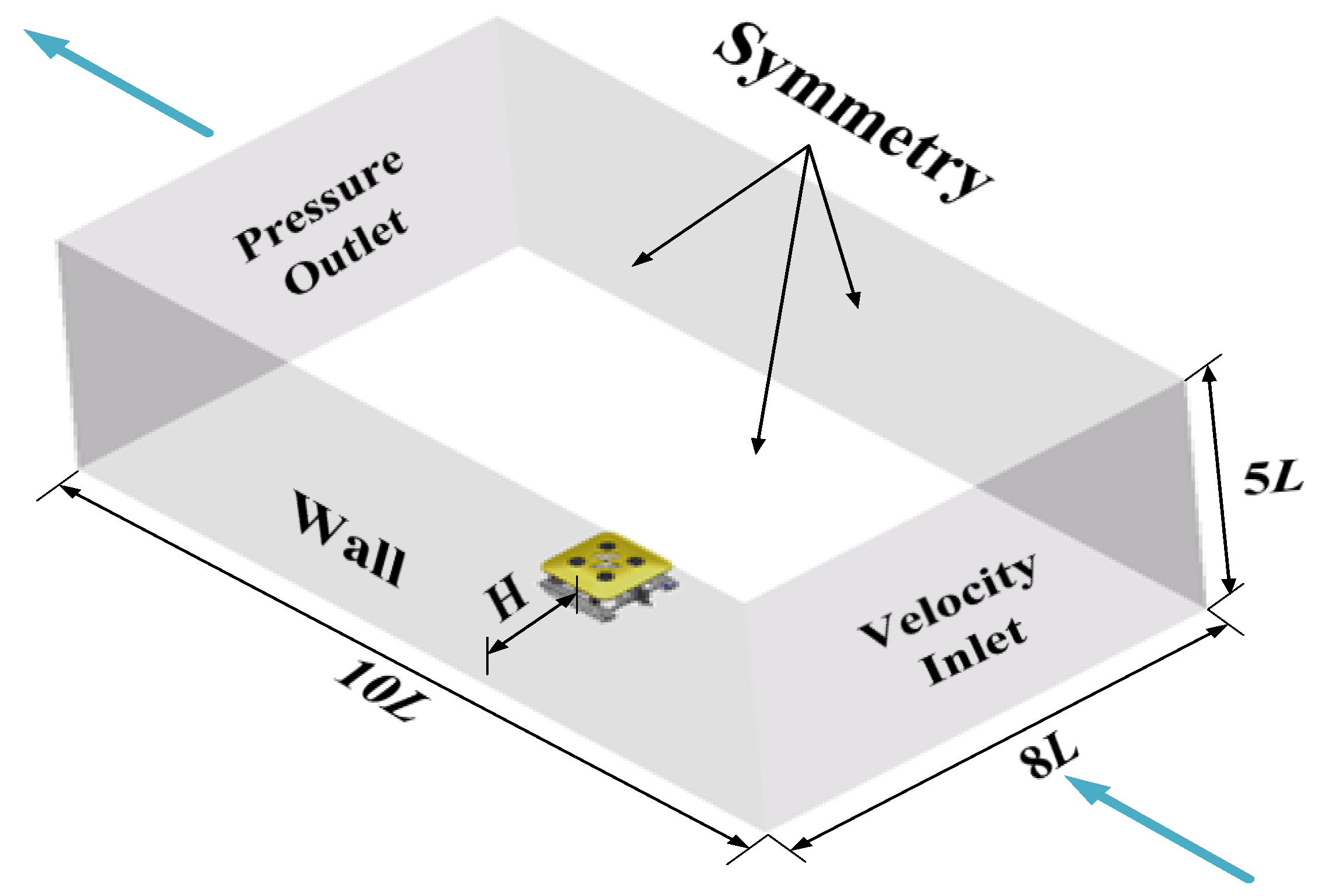
3.2. Computational Model

For the numerical study of the flow field around the ROV, a virtual boundary is constructed to define the computational domain. This boundary acts as a container for the simulation, encapsulating the region where the fluid dynamics are analyzed and the RANS equations are solved. Therefore, boundary conditions must be specified for the spatial domain. This study uses a hexahedral computational domain for simulation, as shown in Figure 2. Assuming the maximum length of the ROV’s structure is L, the fluid domain dimensions are set to 10 L × 8 L × 5 L (length × width × height). The boundary conditions are as follows: the inlet is set as a velocity inlet; the outlet is set as a pressure outlet; the ROV surface and the one side surface are no-slip walls; the remaining boundaries are set as symmetry planes. H is the distance between the wall and the ROV, which can be adjusted to study its influence on the hydrodynamic force.

In the initial phase of hydrodynamic analysis, the primary objective is to understand the interaction between the hull structure and water flow. A critical aspect of this process involves developing a simplified yet accurate propeller model to ensure computational precision and efficiency. Propeller rotation significantly modifies the local flow field, leading to complex phenomena such as high-speed rotation and nonlinear fluid dynamics. To simplify the modeling process while accounting for potential structural- and support-induced disturbances that may introduce additional resistance and flow perturbations, it is common practice to treat the propeller as static when calculating hydrodynamic coefficients. This assumption mitigates the complexities introduced by propeller rotation, thereby facilitating the computation of fundamental hydrodynamic coefficients and aiding in the establishment of a robust hydrodynamic benchmark database. The effects of the propulsion system will be addressed separately in subsequent stages.

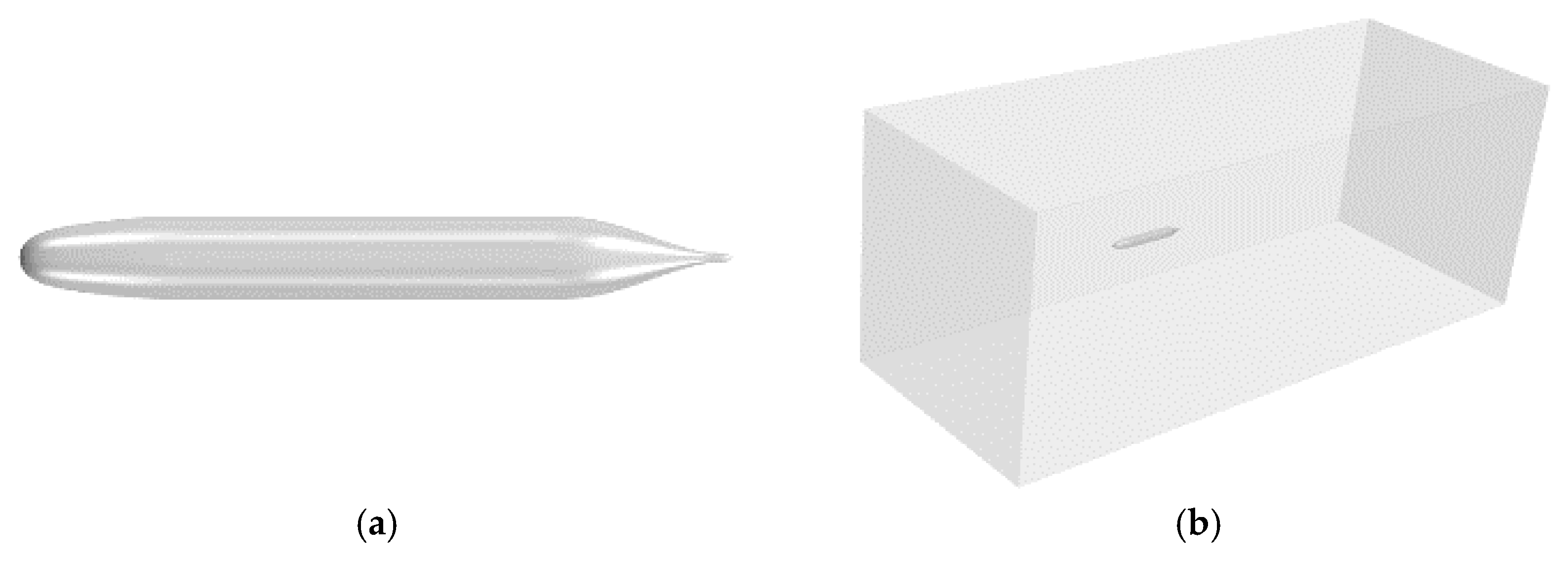
3.3. Grid Generation

The mesh quality has a direct impact on the convergence, precision, and viability of numerical simulations. Structured meshes are advantageous due to their ease of density adjustment and relatively low memory requirements. They also offer significant benefits in addressing boundary layer issues, thereby enhancing the accuracy and reliability of the simulation results. For these reasons, this study employs a hexahedral structured mesh.

The generated mesh is gradually refined as it transitions from the boundary wall toward the ROV surface, which reduces computational time while ensuring simulation accuracy. To capture the boundary layer flow effectively, a prismatic layer mesh is implemented on both the ROV surface and the boundary walls. In all simulation runs, the dimensionless distance (y⁺) of the initial prismatic layer around the ROV and boundary walls is maintained below 1, guaranteeing adequate resolution of the viscous sublayer and precise estimation of the forces and moments exerted on the ROV.

The number of mesh is one of the important factors affecting the accuracy of simulation results and should be given priority after determining the type and size of the meshes in the computational domain. Figure 3 shows the mesh sensitivity analysis results of the longitudinal forces (X) when the ROV moves forward at a speed of 1 m/s with H = 0.4 m. The research indicates that as the number of meshes in the area close to the surface of the ROV increases, the simulation results gradually stabilize. When the total number of meshes reaches 18.8 million, the change of the X tends to be gentle. At this time, the height of the first layer of grids is set to 0.5 mm, and the growth rate is 1.2. After the mesh convergence analysis, the entire computational domain is divided into 18.8 million meshes, and the mesh quality score exceeds 0.5, indicating that the selected meshes have excellent quality characteristics. Figure 4 shows the grid distribution in the area around the ROV when the distance between the ROV and the wall is 0.4 m.

3.4. Validation of the CFDs Method

For the purpose of verifying the CFDs method utilized in our motion simulations, the SUBOFF AFF-1 model provided by DRAPA is adopted as a reference model. This is because the data from the physical towing tests can be retrieved from a comprehensive set of experiments carried out during the research [25]. These data serve as a benchmark for comparing the outcomes of our CFDs simulations, thereby assessing the precision of the CFDs approach. The 3D representation of the SUBOFF model and its flow domain is presented in Figure 5, while the validation outcomes are summarized in

Table 2. Comparison of the total resistance between numerical and experimental results [25] at different speeds.

Speed (m/s)	Our Results (N)	Experimental Results (N)	Error (%)
3.046	85.13	87.4	2.6
5.144	232.54	242.2	4.0
6.091	328.96	332.9	1.2
7.161	445.88	451.5	1.2
8.231	558.62	576.9	3.2

.

In summary, the simulation data align well with the experimental results, exhibiting a relative error of 2–4%, which meets the project’s actual standards. Analysis of the SUBOFF AFF-1 straight-line simulation confirms compliance with engineering standards and verifies the rationality and reliability of the computational theory, meshing approach, and calculation model presented in this paper. Thus, this calculation method is suitable for broader application and can be effectively utilized in future simulation experiments.

4. Wall Hydrodynamic Calculation and Model Establishment for the Complex-Shaped ROV

Considering the influence of the structural asymmetry, cruising speed, and near-wall distance on the hydrodynamic characteristics of the open-frame ROV, this study employs the CFDs method to investigate near-wall motion and determine the wall’s influence range. The multiple linear regression method is used to process the data and extract the relevant wall hydrodynamic coefficients, which are then optimized through parameter sensitivity analysis. A corresponding hydrodynamic mathematical model is established to simulate the effect of the structural asymmetry and near-wall motion on hydrodynamic performance.

4.1. Calculation Condition

In this section, the CFDs method is used to simulate and analyze the hydrodynamic forces acting on an ROV during near-wall motion in the horizontal plane and the vertical plane, respectively. Such research is of great significance for optimizing ROV design, enhancing operational efficiency, and ensuring safety in complex environments.

The main factors influencing the wall hydrodynamic force (F_W) include two key variables: the distance from the wall (H) and the speed of the ROV (V). Specifically, when the ROV approaches the wall, the flow field undergoes significant changes due to the boundary layer effect, leading to variations in the hydrodynamic force. Additionally, the speed of the ROV directly affects the fluid force on the structure. Therefore, the wall hydrodynamic force (F_W) can be regarded as a function of speed (V) and distance (H), i.e., F_W = f(V, H).

To describe this relationship more accurately, we conducted detailed numerical simulations of the ROV’s motion under various conditions. These simulation conditions are summarized in

Table 3. Model simulation cases.

Motion Direction	Primary Factors	Conditions	Case Number
Horizontal plane	The wall distances (H/m)	0.03, 0.05, 0.1, 0.2, 0.4, 0.6, 0.8, 1.0, 1.2, 1.4, 1.7, 2.0, 2.3	130
	The flow velocities (u/m·s−1)	±0.2, ±0.4, ±0.6, ±0.8, ±1.0
Vertical plane	The wall distances (H/m)	0.03, 0.05, 0.1, 0.2, 0.4, 0.6, 0.8, 1.0, 1.2, 1.4, 1.7, 2.0, 2.3	130
	The flow velocities (w/m·s−1)	±0.2, ±0.4, ±0.6, ±0.8, ±1.0

, including key information such as the ROV’s motion direction, speed range, and distance from the wall. Notably, the calculation of positive and negative speeds takes into account the asymmetry of the ROV structure. This asymmetry may cause the ROV to experience different hydrodynamic forces during forward and backward motion, thus requiring separate modeling and analysis.

To validate the proposed method’s effectiveness, we selected a specific case, namely, the near-wall motion of the ROV in the horizontal plane. Through CFDs simulation, we can clearly observe the regular changes in the hydrodynamic force as the ROV’s speed and distance from the wall vary. The specific analysis process for vertical plane motion shares certain similarities with that of the horizontal plane. To avoid repetition, we will not elaborate on it here. The specific numerical results are summarized in

Table 4. Wall hydrodynamic coefficients.

WXu|u|	WXuH	WXuuuH	WXuuuHH	WXww	WXwH	WXwww	WXwwH
−52.25	7.98	52.80	−16.60	−4.82	5.47	−6.74	2.78
WYuu	WYuuH	WYuuHH	WYw	WYH	WYww	WYwH	WYwww
−35.85	75.37	−53.03	−56.49	18.43	−110.17	88.69	−28.23
WZuu	WZuuH	WZuuHH	WZuuHHH	WZw	WZwww	WZwHH	WYwwH
−102.11	278.34	−218.72	51.49	−102.11	−110.04	19.60	52.94
WMuuu	WMuuuH	WMuuuHH	WMw	WMww	WMwH	WMwww	WMwwH
22.63	−36.53	11.79	−2.27	−4.33	5.67	−4.25	1.95
WNuuu	WNuuuH	WNuuuHH	WNwww	WNwwwH	WMwHH
−20.02	22.83	−6.98	−0.93	0.95	−1.57

. By combining theoretical analysis with numerical simulation, we have successfully revealed the variation patterns of the hydrodynamic forces acting on the ROV during near-wall motion. These research findings provide important references for the future design optimization and practical application of ROVs.

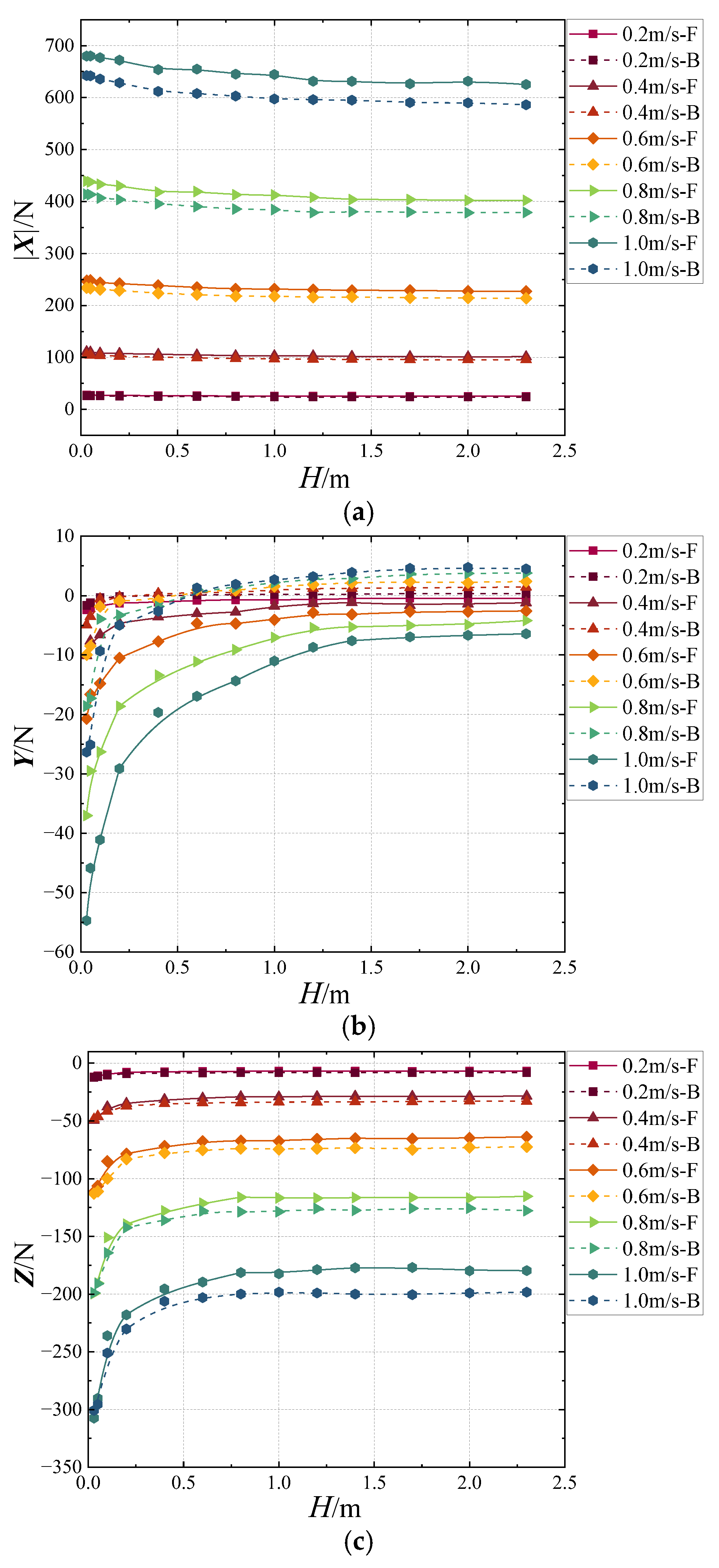
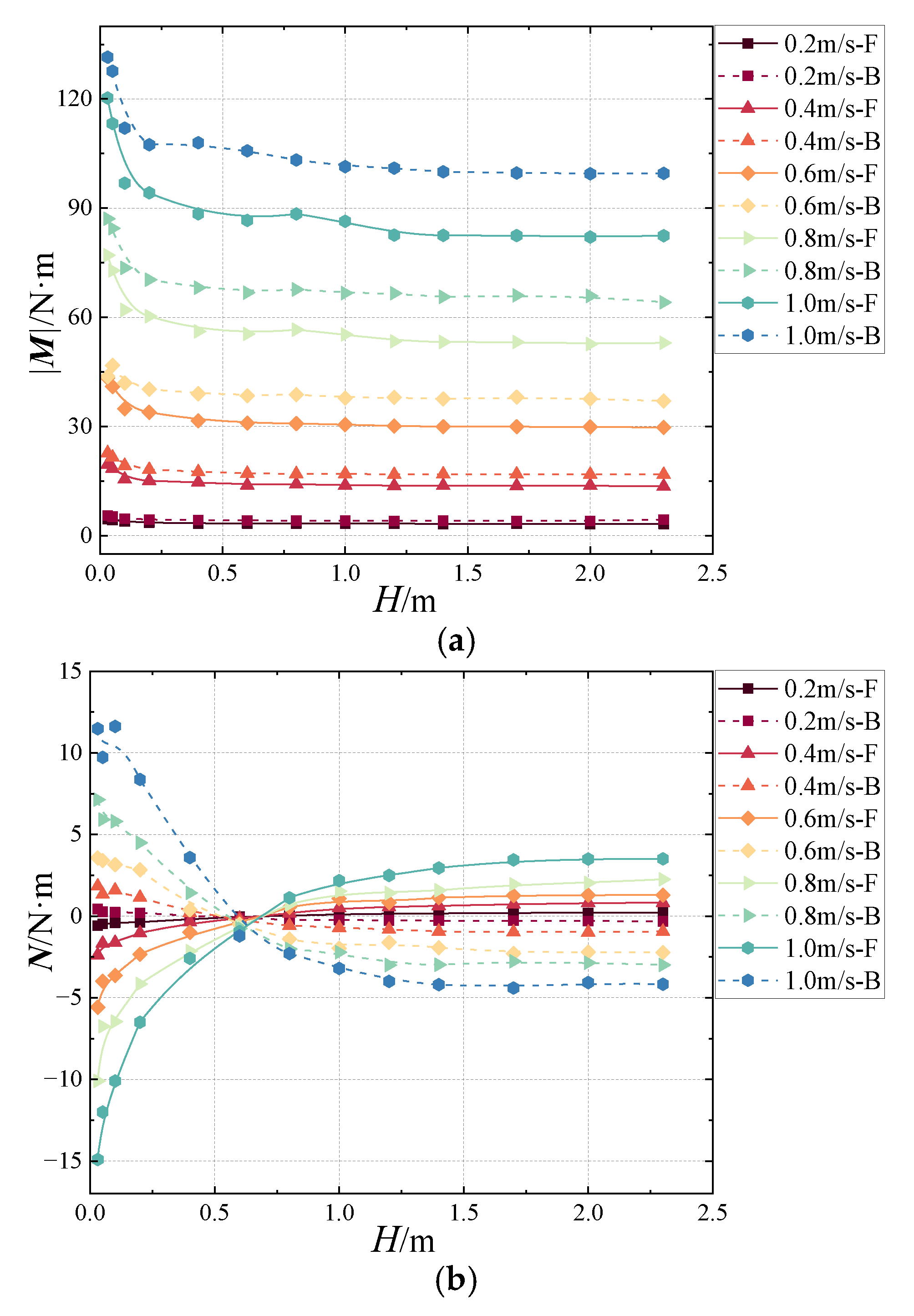
4.2. Calculation Results and Analysis

Figure 6 shows the relationship between the hydrodynamic forces and distance (H) from the wall at various velocities. In this figure, the solid line represents forward motion (denoted as F in the legend), while the dashed line corresponds to backward motion (denoted as B in the legend).

As shown in Figure 6a, the wall has a larger effect on the longitudinal forces (X) for H ≤ 1.4 m. Generally, the X increases markedly as the distance H decreases. This trend can be attributed to the interplay between pressure forces and viscous forces. As depicted in Figure 10, the pressure force rises markedly with decreasing H, whereas the viscous force remains relatively stable. For example, at a velocity of u = 0.4 m/s and a distance of H = 1.4 m, we have X_V = −4.084 N, X_P = −97.866 N (where X_V is the viscous resistance, X_P is the differential pressure resistance); while at the same velocity but with a distance of H = 0.05 m, values are recorded as follows: X_V = −4.361 N, X_P = −106.081 N. These results highlight that the pressure force is highly sensitive to changes in H, whereas the viscous resistance exhibits minimal variation with respect to H. On the other hand, the viscous resistance remains at a low level, it increases with the velocity but is almost independent of H.

In addition to the longitudinal forces, the vertical forces (Z) are also influenced by the proximity to the wall. As illustrated in Figure 6c, the wall exerts a stronger effect on the Z when H ≤ 1.0 m. Similar to the X, the absolute value of Z increases noticeably as H decreases. The underlying mechanism driving this change in the Z mirrors that of the X: the pressure force dominates the variations, while the viscous force plays a secondary role. This observation reinforces the importance of considering wall effects in the design and operation of underwater vehicles, particularly in confined spaces where these forces become more pronounced.

It can be seen from Figure 6b that lateral force (Y) exists from the wall when H ≤ 1.7 m and its absolute value increases rapidly as H decrease. The reason can be found in the velocity contours (Figure 7). At H = 2 m, the velocity field around the ROV is nearly symmetrically distributed in the horizontal plane. This symmetry implies that the flow on either side of the ROV is relatively balanced, resulting in minimal Y acting on the vehicle. However, as the ROV moves closer to the wall, such as at H = 0.05 m, the presence of the wall significantly alters the velocity field. The wall disrupts the flow symmetry, leading to an asymmetric distribution of velocities around the ROV. This asymmetry plays a critical role in generating the lateral force observed in the simulations.

The explanation for this behavior can be derived from Bernoulli’s equation, which relates pressure and velocity in fluid dynamics. As the ROV operates near the wall, the interaction between the wall and the ROV leads to the formation of a high-pressure zone adjacent to the wall. As a result, a pressure differential arises across the ROV, where the pressure on the left side is lower than that on the right side. This pressure disparity creates a lateral force pushing the ROV toward the left (in the opposite direction of the pressure gradient). In the simulation results, this force is indicated by a negative value, as shown in Figure 6b.

To further validate this explanation, we can examine the surface pressure contours of the ROV presented in Figure 8. These contours reveal that when H = 0.05 m, the pressure on the right side of the ROV is significantly higher than the pressure on the left side. Moreover, the pressure on the right side at this proximity is also greater than the pressure observed on the same side when H = 2 m. This indicates that the lateral pressure differential resistance becomes more pronounced as the ROV approaches the wall. In essence, this pressure difference causes the lateral force acting on the ROV to become negative when it operates in close proximity to the wall, as clearly demonstrated in Figure 6b.

In summary, the lateral force experienced by the ROV near the wall is a result of the complex interplay between the wall, the velocity field, and the pressure distribution around the ROV. This phenomenon highlights the importance of considering wall effects in the design and operation of underwater vehicles, particularly in confined environments where these forces can significantly impact maneuverability and stability. Understanding and accurately predicting such forces are essential for optimizing the performance of ROVs in real-world applications.

Figure 9 illustrates the relation between the moments and distance H at different velocities. As shown in Figure 9a, there is a great impact on the pitch moment (M) when H ≤ 1.4 m, with a noticeable increase in M as H decreases. The variation in M follows a similar pattern to the vertical force (Z), as the non-concentration of Z at the centroid results in an increased absolute value of M with decreasing H. The underlying mechanism involves the asymmetry in pressure distribution caused by the proximity to the wall, which generates a torque about the pitch axis.

Similarly, Figure 9b demonstrates that the wall has a large effect on the yaw moments (N) for H ≤ 1.7 m. The absolute value of N typically increases significantly as H decreases. Due to similar reasons as M, both longitudinal and lateral forces not concentrating at the centroid result in an increased absolute value of N with decreasing H. This indicates that the wall’s influence extends beyond translational forces, impacting the rotational stability of the ROV as well.

In addition, as H decreases, the total resistance increases. The effect of the wall on the hydrodynamics of the ROV is also affected by the velocity; specifically, as velocity increases, the resistance caused by changes in distance becomes more significant. This suggests that higher-speed operations near walls require careful consideration of hydrodynamic interactions to ensure stable and efficient performance.

The total resistance acting on the ROV comprises two primary components: pressure difference resistance (Fx) and viscous resistance (Fv). Research indicates that the pressure difference resistance is the main factor influencing the hydrodynamic performance of the ROV (Figure 10a). Conversely, viscous resistance remains at a lower level and increases with velocity, and is almost independent of H, as shown in Figure 10b. This distinction highlights the differing contributions of pressure and viscous forces to the overall resistance experienced by the ROV.

Figure 10. The simulated (a) pressure and (b) viscous resistance of the ROV with different surging velocity at different heights.

Figure 10. The simulated (a) pressure and (b) viscous resistance of the ROV with different surging velocity at different heights.

4.3. Wall Hydrodynamic Mathematical Model

The preceding section demonstrates that the wall force (and moment) is influenced by two primary factors: the velocity (V) and the distance (H) between the ROV and the wall, as mathematically expressed in the equation provided.

$$F_{\mathrm{W}}\left(V,H\right)=F_{\mathrm{H}}-F_{\mathrm{I}}-F_{\mathrm{D}}={\left[\begin{array}{cccccc}{X}_{\mathrm{W}}& Y_{\mathrm{W}}& Z_{\mathrm{W}}& K_{\mathrm{W}}& M_{\mathrm{W}}& N_{\mathrm{W}}\end{array}\right]}^{\mathrm{T}}$$

(11)

Based on the computational results obtained from simulations conducted in both the horizontal and vertical planes, the wall force (and moment) function, along with the associated wall hydrodynamic coefficients, has been derived using the multiple linear regression method. These coefficients are summarized in Table 4. Consequently, a wall hydrodynamic model can be established.

However, it is important to note that not all coefficients contribute equally to the system’s behavior. Some coefficients have a significant impact on the overall dynamics of the ROV, while others exert minimal influence. Therefore, evaluating the effect of coefficient variations on the system becomes crucial. To achieve this, it is necessary to quantify the influence of each coefficient on the system through a numerical metric. This amount is called the coefficient sensitivity. Sensitivity analysis of the hydrodynamic coefficients is subsequently performed to assess their individual contributions to the system’s performance. The sensitivity index serves as a foundation for simplifying the hydrodynamic model, ensuring that only the most influential coefficients are retained.

Sensitivity can be defined in various ways. In this research, since estimations are based on velocities, the change of velocities to the change of a coefficient is defined as the sensitivity of the coefficients. This definition allows for a systematic evaluation of how variations in each coefficient affect the motion parameters of the ROV. The sensitivity relationship is determined through the following structured stages [26]:

• Baseline simulation: perform a simulation of the rotation maneuver using the original set of coefficients without any perturbations and save the resulting data as the baseline reference.
• Coefficient perturbation: Select a specific coefficient, denoted as c_i, and perturb its value by increasing it to (100 + Δ)% of its original value, where Δ = 10%. Then, simulate the rotation maneuver again under these modified conditions.
• Restoration: restore c_i back to its original value to ensure consistency in subsequent steps.
• Repetition: repeat steps (2)–(3) for each coefficient in the model, saving the results for comparison.
• Error calculation: compute the sum of the squares of the differences between the unperturbed baseline data (from step 1) and the perturbed data (from step 2) over the entire simulation time, $\sum (V_P^2-V_{Unp}^2)$.
• Baseline Variance: calculate the sum of the squares of the unperturbed baseline data over the simulation time, $\sum V_{Unp}^2$.
• Sensitivity Index: divide the result from step (5) by the result from step (6) to obtain the sensitivity index for the coefficient under consideration.

$$\mathrm{Sensitivity}={\displaystyle \frac{{\displaystyle \sum \left(V_P^2-V_{Unp}^2\right)}}{{\displaystyle \sum V_{Unp}^2}}}$$

(12)

where V_P and V_Unp are perturbed and unperturbed kinematic parameters of motion, respectively.

The results of sensitivity analysis are illustrated in Figure 11. It is found that some hydrodynamic coefficients have very low sensitivity in this motion state, such as WX_uH, WX_uuuHH, WX_wH, WX_wwH, WY_uuHH, WZ_uuHH, WZ_uuHHH, WZ_wHH, WM_uuuHH, WM_wH, WM_wwH, WM_wHH, WN_uuuHH, and WN_wwwH. Due to their negligible small impact on the ROV’s movement, these coefficients can either be roughly estimated or omitted entirely from the model. This simplification reduces the computational workload significantly while maintaining an acceptable level of accuracy.

Consequently, the viscous hydrodynamic model can be further simplified by retaining only the coefficients with substantial sensitivity. The simplified results are expressed in Equation (13), offering a more efficient and manageable representation of the ROV’s hydrodynamic interactions with the wall. This streamlined model facilitates more accurate predictions and enhances the overall efficiency of motion simulations, particularly in scenarios involving close proximity to walls or boundaries.

$$\begin{array}{l}{X}_W=W{X}_{u\left|u\right|}u\left|u\right|+W{X}_{uuuH}{u}^{3}H+W{X}_{ww}ww+W{X}_{www}{w}^3\\ Y_W=W{Y}_{uu}{u}^2+W{Y}_{uuH}{u}^{2}H+W{Y}_{w}w+W{Y}_{H}H+W{Y}_{ww}{w}^2+W{Y}_{wH}wH+W{Y}_{www}{w}^3+W{Y}_{wwH}^{’}{w}^{2}H\\ Z_{\mathrm{W}}=W{Z}_{uu}{u}^2+W{Z}_{uuH}{u}^{2}H+W{Z}_{w}w+W{Z}_{www}{w}^3\\ M_W=W{M}_{uuu}{u}^3+W{M}_{uuuH}{u}^{3}H+W{M}_{ww}{w}^2+W{M}_{w}w+W{M}_{www}{w}^3\\ N_W=W{N}_{uuu}{u}^3+W{N}_{uuuH}{u}^{3}H+W{N}_{www}{w}^3\end{array}$$

(13)

5. Conclusions

For ROVs equipped with capabilities such as underwater damage detection and repair, autonomous wall-following, and composite drive modes, their maneuvering modes are highly flexible and varied and involve near-wall motion. Furthermore, the influence of complex asymmetric structures on hydrodynamic performance should also be taken into account. To precisely control ROV movement, this study uses CFDs numerical simulation methods to simulate the motion of an asymmetric-structured ROV at different wall distances and speeds. Then, by subtracting the hydrodynamic values of the ROV moving near the wall and the ROV moving in the open water, the wall hydrodynamics caused by the wall effect are obtained. Finally, the hydrodynamic coefficients of the wall are quantified and fitted by multiple linear regression method, and a hydrodynamic model considering the wall hydrodynamic coefficients and the ROV’s structural asymmetry is established.

The results show that during near-wall motion, the wall hydrodynamic force is a major component of the hydrodynamic model and cannot be ignored. When H < 1.4 m, the longitudinal force (X) is significantly influenced by the wall, mainly caused by the change in pressure force, while the influence of viscous resistance is relatively small. The vertical force (Z) and lateral force (Y) increase as H decreases, which is due to the asymmetry of the flow velocity field when close to the wall. According to Bernoulli’s equation, the generation of the lateral force can be attributed to the pressure difference on both sides of the ROV. Additionally, the pitch moment (M) and yaw moment (N) are also affected by the proximity of the wall, and their values increase as H decreases. The total resistance increases with the decrease of H and the increase of speed, where the pressure difference resistance is the dominant factor. In summary, for ROVs moving close to the wall, predicting the wall hydrodynamic force is crucial, especially during the design stage.

References

1. Li, M.; Zhou, H.; Gong, L. Comprehensive Review of ROV Underwater Obstacle Detection and Avoidance Technology. Comput. Eng. Appl. 2024, 60, 34–47. [Google Scholar]
2. Jiang, Z.; Zhao, Y.; Huang, J.; Wang, F.; Chen, Y.; Luo, C.; Luo, G. Development and trends of underwater robots for inspection, maintenance and repair for offshore oil and gas platforms: A review. Sci. Technol. Rev. 2024, 42, 6–15. [Google Scholar]
3. McLean, D.L.; Partridge, J.C.; Bond, T.; Birt, M.J.; Bornt, K.R.; Langlois, T.J. Using industry ROV videos to assess fish associations with subsea pipelines. Cont. Shelf Res. 2017, 141, 76–97. [Google Scholar] [CrossRef]
4. Zhu, A.J.; Ying, L.M.; Zheng, H. Resistance test method on underwater vessel operating close to the bottom or the surface. J. Ship Mech. 2012, 16, 368–374. [Google Scholar]
5. Dunbabin, M.; Roberts, J.; Usher, K.; Winstanley, G.; Corke, P. A hybrid AUV design for shallow water reef navigation. In Proceedings of the 2005 IEEE International Conference on Robotics and Automation, Barcelona, Spain, 18–22 April 2005; pp. 2105–2110. [Google Scholar]
6. Valencia, R.A.; Ramirez, J.A.; Gutierrez, L.B.; Garcia, M.J. Modeling and simulation of an underwater remotely operated vehicle (ROV) for surveillance and inspection of port facilities using CFD tools. In Proceedings of the 27th International Conference on Offshore Mechanics and Archtic Engineering, Estoril, Portugal, 15–20 June 2008; Volume 4, pp. 329–338. [Google Scholar]
7. Ramírez-Macías, J.A.; Brongers, P.; Rúa, S.; Vásquez, R.E. Hydrodynamic modelling for the remotely operated vehicle Visor3 using CFD. IFAC PapersOnLine 2016, 49, 187–192. [Google Scholar] [CrossRef]
8. Katsui, T.; Kajikawa, S.; Inoue, T. Numerical investigation of flow around a rov with crawler based driving system. In Proceedings of the ASME 31st International Conference on Ocean, Offshore and Artic Engineering, Rio de Janeiro, Brazil, 1–6 July 2012; Volume 7, pp. 23–30. [Google Scholar]
9. Baital, M.; Mangkusasmito, F.; Rahmawaty, M.A. Specification Design and Performances Using Computational Fluid Dynamics for Mini-Remotely Operated Underwater Vehicle. Ultim. Comput. J. Sist. Komputer. 2022, 14, 20–27. [Google Scholar] [CrossRef]
10. Rumson, A.G. The application of fully unmanned robotic systems for inspection of subsea pipelines. Ocean. Eng. 2021, 235, 109214. [Google Scholar] [CrossRef]
11. Wang, Z.; Liu, X.; Huang, H. Development of an autonomous underwater helicopter with high maneuverability. Appl. Sci. 2019, 9, 4072. [Google Scholar] [CrossRef]
12. Du, X.X.; Wang, H.; Hao, C.Z. Analysis of hydrodynamic characteristics of unmanned underwater vehicle moving close to the sea bottom. Def. Technol. 2014, 10, 76–81. [Google Scholar] [CrossRef]
13. Mitra, A.; Pandal, J.P.; Warrior, H.V. Experimental and numerical investigation of the hydrodynamic characteristics of Autonomous Underwater Vehicles over sea-beds with complex topography. Ocean. Eng. 2019, 198, 106978. [Google Scholar] [CrossRef]
14. Li, Z.; Tao, J.; Sun, H. Hydrodynamic calculation and analysis of a complex-shaped underwater robot based on computational fluid dynamics and prototype test. Adv. Mech. Eng. 2017, 9, 1–10. [Google Scholar] [CrossRef]
15. Li, X.D.; Hu, Y.L.; Mao, Z.Y.; Tian, W.L. Numerical Simulation of the Hydrodynamic Performance and Self-Propulsion of a UUV near the Seabed. Appl. Sci. 2022, 12, 6975. [Google Scholar] [CrossRef]
16. Wu, B.S.; Xing, F.; Kuang, X.F.; Miao, Q.M. Investigation of hydrodynamic characteristics of submarine moving close to the sea bottom with CFD methods. J. Ship Mech. 2005, 9, 19–28. (In Chinese) [Google Scholar]
17. Xu, S.J.; Han, D.F.; Ma, Q.W. Hydrodynamic forces and moments acting on a remotely operate vehicle with an asymmetric shape moving in a vertical plane. Eur. J. Mech.—B/Fluids 2022, 54, 1–9. [Google Scholar] [CrossRef]
18. Zhang, D.; Zhao, B.; Zhang, Y.; Zhou, N. Numerical simulation of hydrodynamics of ocean-observation-used remotely operated vehicle. Front. Mar. Sci. 2024, 11, 1357144. [Google Scholar] [CrossRef]
19. Zan, Y.F.; Guo, R.N.; Yuan, L.H.; Wang, S.P.; Zhang, D.Z.; Xu, S.J.; Wu, Z.H. Experimental and numerical investigations on the hydrodynamic characteristics of the planar motion of an open-frame remotely operated vehicle. J. Mar. Sci. Technol. 2020, 28, 471–479. [Google Scholar]
20. SNAME. Nomenclature for Treating the Motion of a Submerged Body Through a Fluid; Technical Report Bulletin; Society of Naval Architects and Marine Engineers: New York, NY, USA, 1950; Volume 1–5. [Google Scholar]
21. Fossen, T.I. Handbook of Marine Craft Hydrodynamics and Motion Control; John Wiley & Sons: Hoboken, NJ, USA, 2011. [Google Scholar]
22. Jiang, M.J.; Chen, C.H.; Zhang, L.B. Establishment of hydrodynamic model and research on motion simulation of the open-frame ROV. Chin. J. Ship Res. 2024, 1673–3185. [Google Scholar] [CrossRef]
23. Menter, F.R. Performance of popular turbulence models for attached and separated adverse pressure gradient flows. AIAA J. 1992, 30, 2066–2072. [Google Scholar] [CrossRef]
24. Solkeun, J.; Jongwook, J.; Ray, S.L. Toward Cost-Effective Boundary Layer Transition Computations with Large-Eddy Simulation. J. Fluids Eng. 2018, 140, 111201. [Google Scholar]
25. Huang, T.; Liu, H.L. Measurements of Flows over an Axisymmetric Body with Various Appendages in a Wind Tunnel: The DARPA SUBOFF Experimental Program. In Proceedings of the 19th Symposium on Naval Hydrodynamics, Seoul, Republic of Korea, 23–28 August 1992; National Academy Press: Washington, DC, USA, 1994. Session V. p. 321. [Google Scholar]
26. Farhad, S.; Mansour, R.; Mohammad, D. Estimation of hydrodynamic coefficients and simplification of the depth model of an AUV using CFD and sensitivity analysis. Ocean Eng. 2022, 263, 112369. [Google Scholar]
Figure 1. The 3D model (a) and coordinate systems (b) of the ROV.
Jmse 13 01183 g001
Figure 2. Computational model of the ROV moving close to the wall.
Jmse 13 01183 g002
Figure 3. Curve of the longitudinal forces (X) varying with the number of meshes.
Jmse 13 01183 g003
Figure 4. Mesh of ROV surrounding area. (a) Flow domain mesh. (b) Near-wall and ROV local mesh.
Jmse 13 01183 g004
Figure 5. SUBOFF simulations. (a) SUBOFF model. (b) Flow domain.
Jmse 13 01183 g005
Figure 6. Force results of wall hydrodynamic force simulation. (a) Relation between X and H. (b) Relation between Y and H. (c) Relation between Z and H.
Jmse 13 01183 g006
Figure 7. The velocity contours of the axial plane, u = 0.8 m/s. (a) H = 0.05 m. (b) H = 2 m.
Jmse 13 01183 g007
Figure 8. The pressure contours of the ROV, u = 0.8 m/s. (a) H = 0.05 m, right side. (b) H = 0.05 m, left side. (c) H = 2 m, right side. (d) H = 2 m, left side.
Jmse 13 01183 g008
Figure 9. Moment results of wall hydrodynamic force simulation. (a) Relation between M and H. (b) Relation between N and H.
Jmse 13 01183 g009
Figure 11. Sensitivity analysis.
Jmse 13 01183 g011