Spatial Trajectory Tracking of Underactuated Autonomous Underwater Vehicles by Model–Data-Driven Learning Adaptive Robust Control

Abstract

This paper aims to solve the spatial trajectory tracking control problem of underactuated autonomous underwater vehicles (AUVs) in the presence of system parameter uncertainties and complex external disturbances. To accomplish this goal, a model–data-driven learning adaptive robust control (LARC) strategy is introduced for AUVs. Firstly, a serial iterative learning control (ILC) approach is introduced as feedforward compensation, and then the corresponding trajectory tracking error dynamics model, the Feedforward Compensation–Line of Sight (FFC-LOS) guidance law, and the feedforward compensation-based kinematics controller are designed. Secondly, the dynamics controller is designed for AUVs, which consists of a linear feedback term, a nonlinear robust feedback term, an adjustable model compensation term, and a fast dynamic compensation term. In this control framework, the robust control and fast dynamic compensation parts are utilized to deal with nonlinear uncertainties and disturbances, the projection-type adaptive control part solves the influence caused by the uncertainty of system parameters, and the serial ILC part that is a data-driven learning method can further improve the trajectory tracking accuracy for repetitive tasks. Finally, comparative simulations under different scenarios and different types of disturbances are performed to verify the effectiveness of the proposed control strategy for AUVs.

1. Introduction

Autonomous mobile robots are gradually entering the academic and industrial fields. Autonomous underwater vehicles (AUVs) are sophisticated unmanned systems equipped with advanced perception, decision-making, and operational capabilities, fulfilling critical roles across scientific, commercial, and military sectors. Over the past two decades, there has been a notable surge of interest in AUV research. AUVs are employed in a myriad of applications, including the inspection and monitoring of submarine cables and pipelines, exploration of marine topography, underwater rescue operations, and localization of pollution sources. AUVs adeptly perform a variety of underwater tasks that are often beyond human operational capacity [1,2,3]. To fulfill the requirements of diverse operational missions, AUVs need to demonstrate exceptional capability in trajectory tracking or path following within three-dimensional (3D) environments. Nevertheless, the development of high-performance tracking controllers is significantly complicated by the complex dynamics inherent to AUV systems. These challenges include high degrees of freedom, intrinsic nonlinearities, strong internal coupling, model and parameter uncertainties, and a vulnerability to environmental disturbances. Furthermore, the configuration of the prevalent torpedo-shaped AUVs typically exhibits underactuation, that is, the number of equipped actuators is fewer than the system’s degrees of freedom, imposing additional constraints on controller synthesis. Consequently, the development of advanced control methodologies capable of addressing these multifaceted challenges is of critical importance, as it would substantially enhance the performance and robustness of AUV 3D spatial motion control [4,5,6].

Numerous advanced control strategies have been designed to address the trajectory tracking challenges for AUVs. The existing approaches can be broadly categorized into conventional proportional–integral–derivative (PID) control [7,8], sliding mode control (SMC) [9,10], adaptive control [11,12], robust control [13,14], and intelligent neural network and reinforcement learning control [15,16]. Owing to its structural simplicity and straightforward implementation, PID was initially adopted as a control approach for AUVs. Nevertheless, conventional PID controllers exhibit inherent limitations when addressing dynamic model uncertainties and external disturbances, particularly in complex marine environments. In recent years, the SMC strategy has garnered significant attention for its implementation in AUVs, due to its robustness and adaptation to variations in system dynamics. In Xu et al. [17], a dynamic SMC strategy was presented for trajectory tracking of AUVs. This approach synergistically combines the advantages of SMC with the backstepping technique, thereby improving the vehicle’s resilience to internal uncertainties and external disturbances. In Zhou et al. [18], a terminal SMC method with an RBF neural network was introduced for AUV trajectory tracking control, where the terminal sliding mode method was utilized to design the longitudinal and yaw control law and the neural network was used to address the compound disturbances. Nevertheless, a notable drawback of conventional SMC in practical implementations is the chattering phenomenon, which arises from the discontinuous switching component. Furthermore, robust control and adaptive control have garnered considerable interest from researchers. In Mahapatra and Subudhi [19], a novel robust H-infinity state feedback control scheme was developed for steering control and path following of AUVs in the horizontal plane by tackling the Hamilton–Jacobi–Isaacs equation. Similarly, Zhang et al. [20] proposed robust controllers for the velocity, heading, and depth control of AUVs by integrating H-infinity control theory with Riccati equation solution interpolation. Despite these advancements, there remains a paucity of research and practical cases focused on the application of robust control to 3D spatial trajectory tracking for six-degree-of-freedom AUVs. Additionally, adaptive control is frequently employed in conjunction with other control strategies to enhance the system’s ability to handle uncertainties.

As artificial intelligence technology advances, the application of neural network control and reinforcement learning control in AUVs is gradually being studied. In Luo and Cheng [21], an underactuated AUV trajectory tracking control scheme combining neural network compensation and interference rejection was designed. In this framework, the task of the online neural network was to identify unknown dynamics, including derivatives of virtual control and errors caused by input saturation, in order to improve trajectory tracking performance. In Li et al. [22], an adaptive model-free optimal reinforcement learning control scheme is designed for the trajectory tracking control problem of AUVs with input saturation, where the reinforcement learning strategy based on an actor–critic framework is introduced to approximate the Hamilton–Jacobi–Bellman solution. The primary advantage of reinforcement learning control is its capacity to achieve optimal control by interacting with the environment without dependence on the system model. However, this approach is often constrained by the assumption that model parameters remain invariant throughout the operation. Additionally, the need for extensive data processing and interaction elevate the complexity and computational cost of the algorithm, presenting challenges in practice.

In the works of Yao and Tomizuka [23] and Yao [24], a framework of adaptive robust control (ARC) was established to achieve high performance in controlling nonlinear systems. This control framework integrates the benefits of both adaptive control and robust control, providing effective parametric adaptability while maintaining system robustness against nonlinear uncertainties and disturbances. Additionally, this approach, along with its theoretical advancements, has found applications in areas such as linear motor-driven systems and hydraulic manipulators [25,26,27]. Subsequently, an integrated direct/indirect adaptive robust control (DIARC) framework has been proposed, which optimizes ARC control, ensuring the capability of both parameter adaptive and tracking performance [28]. However, although the control robustness of DIARC and ARC have been guaranteed to a certain extent, there is still room for improvement, especially for repetitive tasks that require high control accuracy. Iterative learning control (ILC) is an intelligent control method commonly used for feedforward compensation, which uses information from previous iteration data to produce optimal control inputs [29,30]. The benefit of ILC is it can achieve effective tracking performance without requiring precise dynamic models, making it particularly valuable for controlling nonlinear and complex systems like AUVs. In the past two decades, ILC has been broadened and implemented in electromechanical systems and robotic systems. However, it remains sensitive to non-repetitive and complex disturbances [31,32]. In addition, there is a lack of research on feedforward control for trajectory tracking of AUVs with a high degree of freedom and underactuated characteristic. Nowadays, it is challenging for underactuated AUVs to achieve high-precision and high-robust trajectory tracking control in 3D space under conditions of uncertain dynamics and complex external disturbances. In particular, there is an urgent need for an intelligent control method that is robust to external disturbances, capable of coping with internal parameter uncertainties, and has good control accuracy to complete certain repetitive tasks.

In this paper, a model–data-driven learning adaptive robust control (LARC) strategy is introduced for spatial trajectory tracking of underactuated AUVs. Compared with other algorithms, the performance of the LARC strategy for AUVs is verified by simulation study and analysis. The main contributions are summarized as follows:

(1)

The serial ILC is introduced as feedforward compensation control, and the corresponding trajectory tracking error dynamics, Feedforward Compensation–Line of Sight (FFC-LOS) guidance law, and feedforward compensation-based kinematics controller are proposed, which can significantly improve trajectory tracking performance for repetitive tasks in 3D space.

(2)

In order to solve the problem of uncertain dynamics parameters, the projection-type adaptation law with rate limits is applied, and the parameter estimation process is designed based on the least squares estimation technique. The nonlinear robust feedback control and fast dynamic compensation term are designed to deal with the nonlinear complex external disturbances.

(3)

The proposed LARC strategy for underactuated AUVs includes the data-driven ILC feedforward part, the adaptive control part, and the robust control and fast dynamic compensation part, using the advantages of both model-based control and data-driven control. The stability of the kinematics controller and dynamics controller are ensured by Lyapunov analysis. The effectiveness of the proposed control strategy is verified by comparison and multi-case study.

The remainder of this paper is organized as follows. Section 2 introduces the mathematical models of the underactuated AUV and control objective. Section 3 presents the controller design, including the ILC compensation part, trajectory tracking error dynamics model, kinematics controller design, and dynamics controller design. Section 4 performs the comprehensive simulation study to verify the effectiveness of the proposed control scheme. The conclusion of this work is illustrated in Section 5.

2. Modeling and Control Objective

2.1. Mathematical Models of Underactuated AUV

In this paper, an underactuated AUV with neutral buoyancy will be studied. Prior to developing the mathematical model for the underactuated AUV, it is essential to define the spatial coordinate system. As shown in Figure 1, three coordinate frames, the earth-fixed inertial reference frame, body-fixed frame, and Serret–Frenet frame, are created and named $\left\{I\right\}$, $\left\{B\right\}$, and $\left\{F\right\}$, respectively. Due to the fact that the roll motion of the underactuated AUV cannot usually be directly controlled by any of its actuators and it is assumed that the hydrodynamic restoring force is sufficiently large in the roll direction, the roll direction motion is ignored.

Notations: Throughout this paper, scalars are represented using standard math fonts; vectors and matrices are denoted with bold math fonts. The primary nomenclatures are presented in Appendix A.

The kinematics model can be established as [33]:

$$\left\{\begin{array}{c}\dot{x}=ucos\psi cos\theta -vsin\psi +wcos\psi sin\theta \hfill \\ \dot{y}=usin\psi cos\theta +vcos\psi +wsin\psi sin\theta \hfill \\ \dot{z}=-usin\theta +wcos\theta \hfill \\ \dot{\theta }=q\hfill \\ \dot{\psi }=r/cos\theta \hfill \end{array}\right.$$

(1)

with ${\mathit{\eta }}_{\mathbf{1}}={\left[x,y,z\right]}^T$ and ${\mathit{\eta }}_{\mathbf{2}}={\left[\theta ,\psi \right]}^T$ as the position vector and attitude vector in the frame $\left\{I\right\}$, respectively. The vectors $\mathit{\upsilon }={\left[u,v,w\right]}^T$ and $\mathit{\omega }={\left[q,r\right]}^T$ are the linear velocity and angular velocity in the frame $\left\{B\right\}$, respectively.

The dynamics model of the underactuated AUV can be established as [33,34]:

$$\left\{\begin{array}{c}{m}_{11}\dot{u}=m_{22}vr-m_{33}wq-X_{u}u-X_{u\left|u\right|}u\left|u\right|+{\tau }_1+D_u\hfill \\ m_{22}\dot{v}=-m_{11}ur-Y_{v}v-Y_{v\left|v\right|}v\left|v\right|+D_v\hfill \\ m_{33}\dot{w}=m_{11}uq-Z_{w}w-Z_{w\left|w\right|}w\left|w\right|+D_w\hfill \\ m_{55}\dot{q}=\left(m_{33}-m_{11}\right)uw-M_{q}q-M_{q\left|q\right|}q\left|q\right|-\left(z_{G}W-z_{B}B\right)sin\theta +{\tau }_2+D_q\hfill \\ m_{66}\dot{r}=-\left(m_{22}-m_{11}\right)uv-N_{r}r-N_{r\left|r\right|}r\left|r\right|+{\tau }_3+D_r\hfill \end{array}\right.$$

(2)

where $m_{ii}\left(i=1,2,3,5,6\right)$ denotes the combined terms of inertia and added mass. $X_u$, $Y_v$, $Z_w$, $M_q$, and $N_r$ represent the hydrodynamic coefficients associated with the linear drag terms, while $X_{u\left|u\right|}$, $Y_{v\left|v\right|}$, $Z_{w\left|w\right|}$, $M_{q\left|q\right|}$, and $N_{r\left|r\right|}$ correspond to the coefficients for the nonlinear drag terms. ${\tau }_1$ is the propeller thrust. ${\tau }_2$ and ${\tau }_3$ are the pitch and yaw torques produced by the rudders, respectively. $D_u$, $D_v$, $D_w$, $D_q$, and $D_r$ indicate the oceanic external disturbance.

Assumption 1.

The AUV utilized in this paper features a uniform mass distribution and it is symmetrical about three principal axial planes. Considering that the pitch angle of the AUV cannot be too large during the 3D trajectory tracking process, otherwise it will lose basic stability, the pitch angle is constrained to the range of $-{30}^{\circ }\le \theta \le {30}^{\circ }$. The uncertain disturbances $D_u$, $D_v$, $D_w$, $D_q$, and $D_r$ are bounded with known values.

Assumption 2.

Considering that the actual propeller thrust and rudder torques cannot be too large to meet the actual engineering conditions, the control inputs for the AUV are subject to limitations, which means that there exist positive known constants ${\tau }_{1max}$, ${\tau }_{2max}$, and ${\tau }_{3max}$ such that $0\le {\tau }_1\le {\tau }_{1max}$, $|{\tau }_2| \le {\tau }_{2max}$, and $|{\tau }_3| \le {\tau }_{3max}$.

Assumption 3.

The vehicle velocities, angular velocities, and their derivatives are also bounded to better fit practice, which means that there exist positive known constants ${\epsilon }_{imax}\left(i=1,2,3,5,6\right)$ and ${\nu }_{imax}\left(i=1,2,3,5,6\right)$ such that $0\le u\le {\epsilon }_{1max}$, $\left|v\right|\le {\epsilon }_{2max}$, $\left|w\right|\le {\epsilon }_{3max}$, $\left|q\right|\le {\epsilon }_{5max}$, $\left|r\right|\le {\epsilon }_{6max}$, $|\dot{u}| \le {\nu }_{1max}$, $|\dot{v}| \le {\nu }_{2max}$, $|\dot{w}| \le {\nu }_{3max}$, $|\dot{q}| \le {\nu }_{5max}$, and $|\dot{r}| \le {\nu }_{6max}$.

2.2. Control Objective

In the trajectory tracking task, the underactuated AUV is required to gradually track the predefined trajectory which is bounded and differentiable. Moreover, the reference trajectory only focuses on path kinematics and does not involve path dynamics. As shown in Figure 1, the position of the moving point P on the desired trajectory is denoted as ${\mathit{\eta }}_{\mathbf{1}\mathit{d}}={\left[x_d,y_d,z_d\right]}^T$, and the corresponding route angles at point P are defined as ${\mathit{\eta }}_{\mathbf{2}\mathit{d}}={\left[{\theta }_d,{\psi }_d\right]}^T$ with ${\theta }_d=arctan\left(-{\dot{z}}_d/\sqrt{{\dot{x}}_d^2+{\dot{y}}_d^2}\right)$ and ${\psi }_d=\mathrm{atan}2\left({\dot{y}}_d,{\dot{x}}_d\right)$.

In practice, the elevation angle ${\theta }_b$ of the vehicle also includes the attack angle $\alpha =arctan\left(-w/u\right)$; the course angle ${\psi }_b$ of the vehicle consists of the sideslip angle $\beta =arctan\left(v/\sqrt{u^2+w^2}\right)$ as well, which can be expressed as ${\theta }_b=\theta +\alpha$ and ${\psi }_b=\psi +\beta$. The control objective of spatial trajectory tracking is to develop an effective control law so that the tracking error between the posture of the vehicle and the desired trajectory can be well controlled.

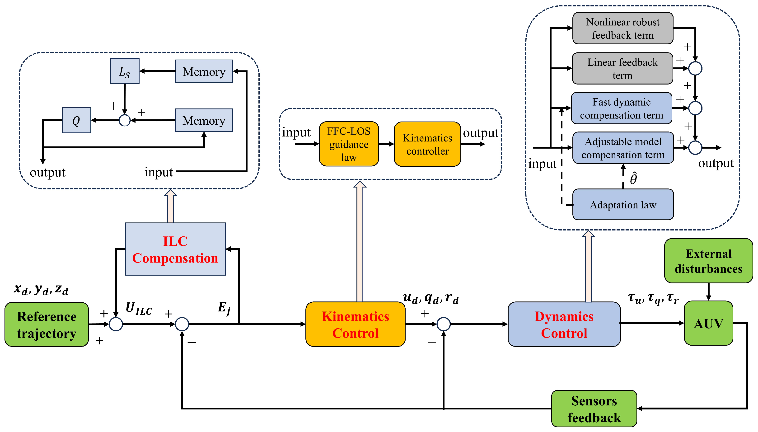
3. Controller Design

In order to accomplish the control goal, the process of the controller design can be decomposed into the two sub-stages. The first sub-stage is to develop a valid virtual control law ${\left[u_d,q_d,r_d\right]}^T$, and the second sub-stage is to design a highly robust control law ${\left[{\tau }_1,{\tau }_2,{\tau }_3\right]}^T$ in the presence of system parameter uncertainties and external disturbances. The proposed LARC scheme for the underactuated AUV in this paper is shown in Figure 2. In kinematics controller design, serial ILC feedforward compensation is adopted. Accordingly, the ILC-based trajectory tracking error dynamics model, the FFC-LOS guidance law, and the corresponding kinematics controller are developed. In dynamics controller design, the projection-type adaptation law and the robust control law for the underactuated AUV are designed to improve the adaptive and anti-disturbance performances of the vehicle. The whole control strategy utilizes the advantages of model-based control and data-driven control.

3.1. ILC Part in Kinematics Controller

ILC provides excellent stable tracking performance without requiring an accurate system model. As illustrated in Figure 2, the serial ILC structure that serves as feedforward compensation iteratively learns to generate inputs to adjust the kinematics controller reference before the closed-loop system.

The tracking error $E_j\left(s\right)$ at the jth iteration of the serial ILC can be expressed as

$$E_j\left(s\right)=R\left(s\right)-C\left(s\right)\left[R\left(s\right)+U_{\mathrm{ILC},j}\left(s\right)\right]$$

(3)

with $C\left(s\right)$ as the closed-loop system transfer function, $R\left(s\right)$ as the reference trajectory, and $U_{\mathrm{ILC},j}\left(s\right)$ as the compensation in the jth iteration.

The serial ILC-based learning law $U_{\mathrm{ILC},j+1}$ for the next iteration can be written as

$$U_{\mathrm{ILC},j+1}\left(s\right)=Q\left(s\right)\left[U_{\mathrm{ILC},j}+L_s{E}_j\left(s\right)\right]$$

(4)

where $L_s\in \left(0,1\right]$ is the learning gain to produce the desired ILC input in the next iteration, and $Q\left(s\right)$ is the Q filter that limits the learning bandwidth to achieve robustness.

Asymptotic stability and convergence of the serial ILC-based learning law described in (4) can be guaranteed and the details have already been presented in Bristow et al. [31].

3.2. Trajectory Tracking Error Dynamics Model

Before designing the kinematics controller, the trajectory tracking error dynamics model embedded by ILC needs to be established. Through the serial ILC, there exists an adjusted desired trajectory ${\left[x_d+x_{\mathrm{ILC}},y_d+y_{\mathrm{ILC}},z_d+z_{\mathrm{ILC}}\right]}^T$ that should be followed by the kinematics controller and dynamics controller. The adjusted trajectory tracking error ${\mathit{\eta }}_{\mathbf{1}\mathit{e}}^{\prime }={\left[x_e^{\prime },y_e^{\prime },z_e^{\prime }\right]}^T$ in the frame $\left\{F\right\}$ can be expressed as

$$\begin{gathered} {\mathit{\eta }}_{\mathbf{1}\mathit{e}}^{\prime }={\mathit{\eta }}_{\mathbf{1}\mathit{e}}-{\mathit{\eta }}_{\mathbf{ILC}}={\left[\begin{array}{ccc}cos{\psi }_{d}cos{\theta }_d& -sin{\psi }_d& cos{\psi }_{d}sin{\theta }_d\\ sin{\psi }_{d}cos{\theta }_d& cos{\psi }_d& sin{\psi }_{d}sin{\theta }_d\\ -sin{\theta }_d& 0& cos{\theta }_d\end{array}\right]}^T\left[\begin{array}{c}x-x_d\\ y-y_d\\ z-z_d\end{array}\right] \\ -{\left[\begin{array}{ccc}cos{\psi }_{d}cos{\theta }_d& -sin{\psi }_d& cos{\psi }_{d}sin{\theta }_d\\ sin{\psi }_{d}cos{\theta }_d& cos{\psi }_d& sin{\psi }_{d}sin{\theta }_d\\ -sin{\theta }_d& 0& cos{\theta }_d\end{array}\right]}^T\left[\begin{array}{c}{x}_{\mathrm{ILC}}\\ y_{\mathrm{ILC}}\\ z_{\mathrm{ILC}}\end{array}\right] \end{gathered}$$

(5)

where $x_e^{\prime }$, $y_e^{\prime }$, and $z_e^{\prime }$ represent the along-track error, cross-track error, and vertical-track error, respectively, ${\mathit{\eta }}_{\mathbf{1}\mathit{e}}={\left[x_e,y_e,z_e\right]}^T$ is the original position tracking error, and ${\mathit{\eta }}_{\mathbf{ILC}}={\left[s_{\mathrm{ILC}},h_{\mathrm{ILC}},e_{\mathrm{ILC}}\right]}^T$ is the compensation term in the frame $\left\{F\right\}$.

Differentiating (5) yields

$${\dot{\mathit{\eta }}}_{\mathbf{1}\mathit{e}}^{\prime }={{\mathit{S}}_{\mathit{F}}}^T\left({\mathit{\eta }}_{\mathbf{1}\mathit{e}}-{\mathit{\eta }}_{\mathbf{ILC}}\right)+{\mathit{R}}_{\mathit{V}}^{\mathit{F}}{\mathit{U}}_{\mathit{V}}-{\mathit{V}}_{\mathit{d}}$$

(6)

with ${\mathit{V}}_{\mathit{d}}={\left[U_d,0,0\right]}^T$ and $U_d=\sqrt{{\dot{x}}_d^2+{\dot{y}}_d^2+{\dot{z}}_d^2}$ as the resultant velocity of the moving point P, and ${\mathit{U}}_{\mathit{V}}={\left[U,0,0\right]}^T$ and $U=\sqrt{u^2+v^2+w^2}$ as the resultant velocity of the vehicle. The skew-symmetric matrix ${\mathit{S}}_{\mathit{F}}$ and rotation matrix ${\mathit{R}}_{\mathit{V}}^{\mathit{F}}$ are calculated as [35]:

$${\mathit{S}}_{\mathit{F}}=\left[\begin{array}{ccc}0& -{\dot{\psi }}_{d}cos{\theta }_d& {\dot{\theta }}_d\\ {\dot{\psi }}_{d}cos{\theta }_d& 0& {\dot{\psi }}_{d}sin{\theta }_d\\ -{\dot{\theta }}_d& -{\dot{\psi }}_{d}sin{\theta }_d& 0\end{array}\right]$$

(7)

$${\mathit{R}}_{\mathit{V}}^{\mathit{F}}=\left[\begin{array}{ccc}cos{\psi }_{e}cos{\theta }_e& -sin{\psi }_e& cos{\psi }_{e}sin{\theta }_e\\ sin{\psi }_{e}cos{\theta }_e& cos{\psi }_e& sin{\psi }_{e}sin{\theta }_e\\ -sin{\theta }_e& 0& cos{\theta }_e\end{array}\right]$$

(8)

In addition, the angle tracking errors can be formulated by

$${\mathit{\eta }}_{\mathbf{2}\mathit{e}}=\left[\begin{array}{c}{\theta }_e\\ {\psi }_e\end{array}\right]=\left[\begin{array}{c}{\theta }_b-{\theta }_d\\ {\psi }_b-{\psi }_d\end{array}\right]$$

(9)

Furthermore, by expanding $\left(6\right)$ and differentiating $\left(9\right)$, the error dynamics model can be written as

$$\left\{\begin{array}{c}{\dot{x}}_e^{\prime }=\left(y_e-h_{\mathrm{ILC}}\right){\dot{\psi }}_{d}cos{\theta }_d-\left(z_e-e_{\mathrm{ILC}}\right){\dot{\theta }}_d+Ucos{\psi }_{e}cos{\theta }_e-U_d\hfill \\ {\dot{y}}_e^{\prime }=\left(-x_e+s_{\mathrm{ILC}}\right){\dot{\psi }}_{d}cos{\theta }_d-\left(z_e-e_{\mathrm{ILC}}\right){\dot{\psi }}_{d}sin{\theta }_d+Usin{\psi }_{e}cos{\theta }_e\hfill \\ {\dot{z}}_e^{\prime }=\left(x_e-s_{\mathrm{ILC}}\right){\dot{\theta }}_d+\left(y_e-h_{\mathrm{ILC}}\right){\dot{\psi }}_{d}sin{\theta }_d-Usin{\theta }_e\hfill \\ {\dot{\theta }}_e=q+\dot{\alpha }-{\dot{\theta }}_d\hfill \\ {\dot{\psi }}_e=r/cos\theta +\dot{\beta }-{\dot{\psi }}_d\hfill \end{array}\right.$$

(10)

The above trajectory tracking error dynamics model is the basis for designing the kinematics controller. It is worth noting that the adjusted desired trajectory mentioned here is used to design a controller with higher control accuracy and robustness. In fact, the control’s purpose is still to render the trajectory of the vehicle as able to track the predefined desired trajectory, which is usually generated by the planning and navigation system, as described in Section 2.2.

3.3. Kinematics Controller Design

The kinematics control law is designed as

$$\left\{\begin{array}{cc}\hfill u_d=& \left[-k_1\left(x_e-s_{\mathrm{ILC}}\right)+U_d\right]{\displaystyle \frac{cos\alpha cos\beta }{cos{\theta }_{e}cos{\psi }_e}}\hfill \\ \hfill q_d=& -\dot{\alpha }+{\dot{\theta }}_d+{\dot{\theta }}_{\mathrm{FFC}-\mathrm{LOS}}-k_2\left({\theta }_e-{\theta }_{\mathrm{FFC}-\mathrm{LOS}}\right)+\left(z_e-e_{\mathrm{ILC}}\right)U{\displaystyle \frac{sin{\theta }_e-sin{\theta }_{\mathrm{FFC}-\mathrm{LOS}}}{{\theta }_e-{\theta }_{\mathrm{FFC}-\mathrm{LOS}}}}\hfill \\ \hfill r_d=& cos\theta \left[-\dot{\beta }+{\dot{\psi }}_d+{\dot{\psi }}_{\mathrm{FFC}-\mathrm{LOS}}-k_3\left({\psi }_e-{\psi }_{\mathrm{FFC}-\mathrm{LOS}}\right)-\left(y_e-h_{\mathrm{ILC}}\right)Ucos{\theta }_e{\displaystyle \frac{sin{\psi }_e-sin{\psi }_{\mathrm{FFC}-\mathrm{LOS}}}{{\psi }_e-{\psi }_{\mathrm{FFC}-\mathrm{LOS}}}}\right]\hfill \end{array}\right.$$

(11)

where $k_1,k_2,k_3>0$ are the designed control parameters. In addition, the following is held for the kinematics controller [36]:

$$\underset{a\to b}{lim}{\displaystyle \frac{sina-sinb}{a-b}}\stackrel{\nabla =a-b}{\to }\underset{\nabla \to 0}{lim}{\displaystyle \frac{sina-sin(a-\nabla )}{\nabla }}=cosa$$

(12)

The designed FFC-LOS guidance law ${\theta }_{\mathrm{FFC}-\mathrm{LOS}}$ and ${\psi }_{\mathrm{FFC}-\mathrm{LOS}}$ can be expressed as

$$\left\{\begin{array}{c}{\theta }_{\mathrm{FFC}-\mathrm{LOS}}=arctan\left({\displaystyle \frac{z_e-e_{\mathrm{ILC}}}{{\mathrm{\Delta }}_z}}\right)\hfill \\ {\psi }_{\mathrm{FFC}-\mathrm{LOS}}=arctan\left({\displaystyle \frac{-y_e+h_{\mathrm{ILC}}}{{\mathrm{\Delta }}_y}}\right)\hfill \end{array}\right.$$

(13)

where ${\mathrm{\Delta }}_z>0$ and ${\mathrm{\Delta }}_y>0$ are the designed guidance gain coefficients. The stability analysis of the kinematics subsystem is shown in Appendix B.

3.4. Dynamics Controller Design

In order to solve the sub-problem of dynamics control, the surge velocity tracking controller, pitch angular velocity tracking controller, and yaw angular velocity tracking controller are designed, respectively, to produce the final control inputs from the propeller and rudders of the vehicle. Herein, the dynamic controller is designed based on DIARC, which simultaneously executes robust control law and adaptive law to improve the vehicle’s ability to resist external disturbances and system parameter uncertainties.

3.4.1. Parameter Adaptation Law

In practice, accurately determining the system parameters of the vehicle is challenging. To mitigate these adverse effects, integrating an adaptation law along with a parameter estimation technique into the design of the control law can be beneficial. In the design of the dynamics controller, the robust controller, adaptation law, and estimation algorithm are synthesized.

Firstly, the adaptation law with rate limits is utilized. For any vector $\mathit{\zeta }$ and pre-set rate limit ${\dot{\theta }}_M$, the saturation function is defined as

$$sa{t}_{{\dot{\theta }}_M}\left(\mathit{\zeta }\right)=s_0\mathit{\zeta },s_0=\left\{\begin{array}{cc}1,\hfill & \parallel \mathit{\zeta }\parallel \le {\dot{\theta }}_M\hfill \\ {\displaystyle \frac{{\dot{\theta }}_M}{\parallel \mathit{\zeta }\parallel }},\hfill & \parallel \mathit{\zeta }\parallel >{\dot{\theta }}_M\hfill \end{array}\right.$$

(14)

Then, the following projection-type adaptation law with rate limits can be expressed as

$${\stackrel{.}{\widehat{\mathit{\theta }}}}_{\mathit{i}}=sa{t}_{{\dot{\theta }}_{Mi}}\left(Pro{j}_{{\widehat{\mathit{\theta }}}_{\mathit{i}}}\left({\mathbf{\Gamma }}_{\mathit{i}}{\mathit{\mu }}_{\mathit{i}}\right)\right),{\widehat{\mathit{\theta }}}_{\mathit{i}}\left(0\right)\in {\mathbf{\Omega }}_{{\mathit{\theta }}_{\mathit{i}}}$$

(15)

where ${\widehat{\mathit{\theta }}}_{\mathit{i}}\left(i=1,2,3\right)$ is the estimation value of ${\mathit{\theta }}_{\mathit{i}}\left(i=1,2,3\right)$, ${\dot{\theta }}_{Mi}\left(i=1,2,3\right)$ is the pre-set rate limit for each ${\mathit{\theta }}_{\mathit{i}}$, ${\mathbf{\Gamma }}_{\mathit{i}}\left(i=1,2,3\right)$ is the positive adaptation rate matrix, and ${\mathit{\mu }}_{\mathit{i}}\left(i=1,2,3\right)$ is the vector of adaptation function to be determined later. In addition, ${\mathit{\theta }}_{\mathit{imax}}\left(i=1,2,3\right)$ and ${\mathit{\theta }}_{\mathit{imin}}\left(i=1,2,3\right)$ are the known maximum and minimum values of ${\mathit{\theta }}_{\mathit{i}}$. Furthermore, the following standard projection mapping is utilized in the adaptation process [37]:

$$Pro{j}_{{\widehat{\mathit{\theta }}}_{\mathit{i}}}\left({\mathit{\zeta }}_{\mathit{i}}\right)=\left\{\begin{array}{c}{\mathit{\zeta }}_{\mathit{i}},\mathrm{if}{\widehat{\mathit{\theta }}}_{\mathit{i}}\in {\overline{\mathbf{\Omega }}}_{{\mathit{\theta }}_{\mathit{i}}}\mathrm{or}\left({\widehat{\mathit{\theta }}}_{\mathit{i}}\in \mathbf{\partial }{\mathbf{\Omega }}_{{\mathit{\theta }}_{\mathit{i}}}\mathrm{and}{{\mathit{n}}_{{\widehat{\mathit{\theta }}}_{\mathit{i}}}}^T{\mathit{\zeta }}_{\mathit{i}}\le 0\right)\hfill \\ \left(\mathit{I}-{\mathbf{\Gamma }}_i{\displaystyle \frac{{\mathit{n}}_{{\widehat{\mathit{\theta }}}_{\mathit{i}}}{{\mathit{n}}_{{\widehat{\mathit{\theta }}}_{\mathit{i}}}}^T}{{{\mathit{n}}_{{\widehat{\mathit{\theta }}}_{\mathit{i}}}}^T{\mathbf{\Gamma }}_{\mathit{i}}{\mathit{n}}_{{\widehat{\mathit{\theta }}}_{\mathit{i}}}}}\right){\mathit{\zeta }}_{\mathit{i}},\mathrm{if}{\widehat{\mathit{\theta }}}_{\mathit{i}}\in \mathbf{\partial }{\mathbf{\Omega }}_{{\mathit{\theta }}_{\mathit{i}}}\mathrm{and}{{\mathit{n}}_{{\widehat{\mathit{\theta }}}_{\mathit{i}}}}^T{\mathit{\zeta }}_{\mathit{i}}>0\hfill \end{array}\right.$$

(16)

where ${\mathit{\zeta }}_{\mathit{i}}\left(i=1,2,3\right)$ is the function to be projected, ${\overline{\mathbf{\Omega }}}_{{\mathit{\theta }}_{\mathit{i}}}\left(i=1,2,3\right)$ and $\mathbf{\partial }{\mathbf{\Omega }}_{{\mathit{\theta }}_{\mathit{i}}}\left(i=1,2,3\right)$ are the interior and boundary of the set ${\mathbf{\Omega }}_{{\mathit{\theta }}_{\mathit{i}}}\left(i=1,2,3\right)$, and ${\mathit{n}}_{{\widehat{\mathit{\theta }}}_{\mathit{i}}}\left(i=1,2,3\right)$ is the outward unit normal vector at ${\widehat{\mathit{\theta }}}_{\mathit{i}}\in \mathbf{\partial }{\mathbf{\Omega }}_{{\mathit{\theta }}_{\mathit{i}}}$.

The parameter estimation error is denoted as ${\tilde{\mathit{\theta }}}_{\mathit{i}}={\widehat{\mathit{\theta }}}_{\mathit{i}}-{\mathit{\theta }}_{\mathit{i}}\left(i=1,2,3\right)$. With the above parameter adaptation law, the following properties can be held [38]:

$$\begin{array}{cc}\hfill & P1:{\widehat{\mathit{\theta }}}_{\mathit{i}}\in {\mathbf{\Omega }}_{{\mathit{\theta }}_{\mathit{i}}}\triangleq \left\{{\widehat{\mathit{\theta }}}_{\mathit{i}}:{\mathit{\theta }}_{\mathit{imin}}\le {\widehat{\mathit{\theta }}}_{\mathit{i}}\le {\mathit{\theta }}_{\mathit{imax}}\right\}\hfill \\ \hfill & P2:{{\tilde{\mathit{\theta }}}_{\mathit{i}}}^T\left[{\mathbf{\Gamma }}_{\mathit{i}}^{-1}Pro{j}_{{\widehat{\mathit{\theta }}}_{\mathit{i}}}\left({\mathrm{\Gamma }}_{\mathit{i}}{\mathit{\mu }}_{\mathit{i}}\right)-{\mathit{\mu }}_{\mathit{i}}\right]\le 0,\forall {\mathit{\mu }}_{\mathit{i}}\hfill \\ \hfill & P3:\parallel {\stackrel{.}{\widehat{\mathit{\theta }}}}_{\mathit{i}}\left(t\right)\parallel \le {\dot{\theta }}_{Mi},\forall t\hfill \end{array}$$

(17)

3.4.2. Velocity Tracking Controller Design

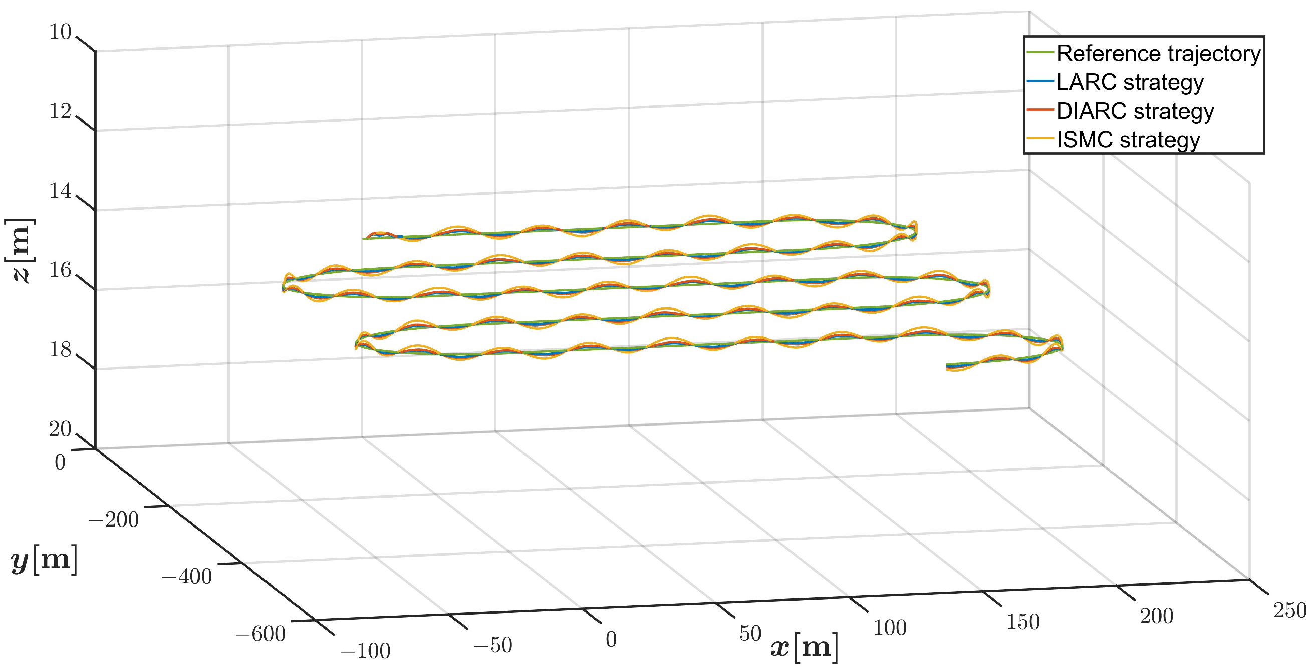
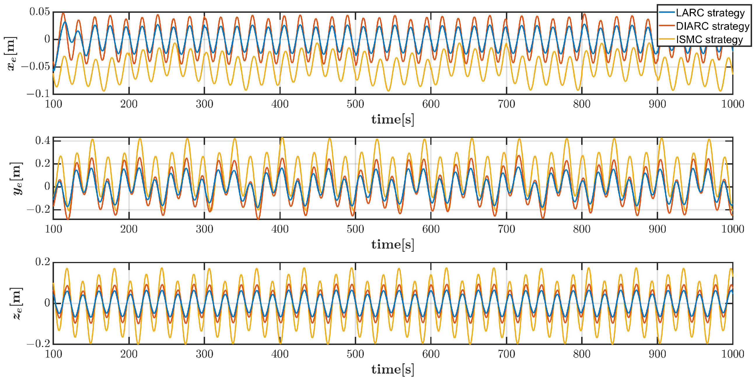
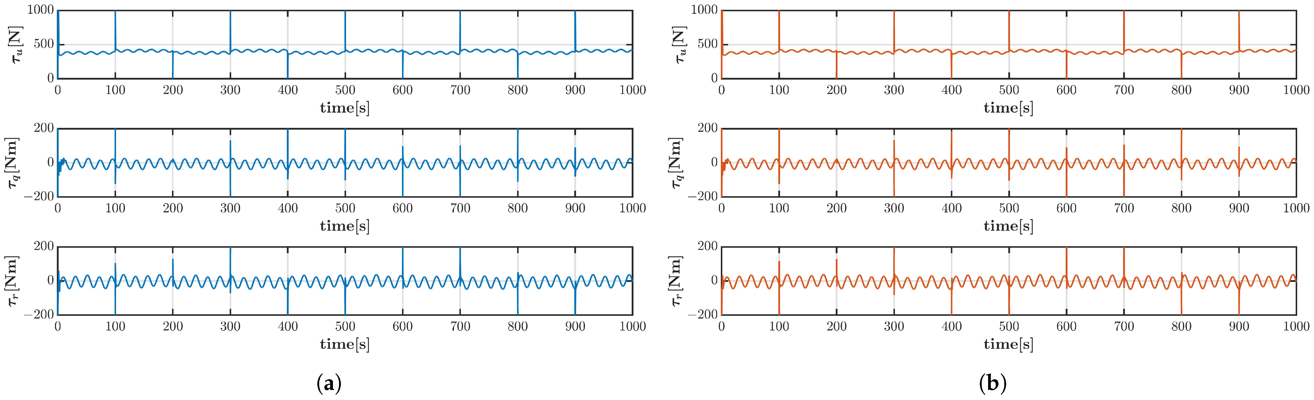
Define the surge velocity tracking error, pitch angular velocity tracking error, and yaw angular velocity tracking error as

$$e_1=u-u_d,e_2=q-q_d,e_3=r-r_d$$

(18)

Then, the dynamics equations of the vehicle can be written in a more compact form:

$$\begin{array}{cc}\hfill & {\theta }_{15}{\dot{e}}_1={\mathit{\varphi }}_{\mathbf{1}}^T{\mathit{\theta }}_{\mathbf{1}}+{\tau }_1+D_u\hfill \\ \hfill & {\theta }_{25}{\dot{e}}_2={\mathit{\varphi }}_{\mathbf{2}}^T{\mathit{\theta }}_{\mathbf{2}}+{\tau }_2+D_q\hfill \\ \hfill & {\theta }_{34}{\dot{e}}_3={\mathit{\varphi }}_{\mathbf{3}}^T{\mathit{\theta }}_{\mathbf{3}}+{\tau }_3+D_r\hfill \end{array}$$

(19)

with the regressor vectors

$$\begin{array}{cc}\hfill & {\mathit{\varphi }}_{\mathbf{1}}={\left[\begin{array}{c}vr,-wq,-u,-u\left|u\right|,-{\dot{u}}_d\end{array}\right]}^T\hfill \\ \hfill & {\mathit{\varphi }}_{\mathbf{2}}={\left[\begin{array}{c}uw,-q,-q\left|q\right|,-sin\theta ,-{\dot{q}}_d\end{array}\right]}^T\hfill \\ \hfill & {\mathit{\varphi }}_{\mathbf{3}}={\left[\begin{array}{c}-uv,-r,-r\left|r\right|,-{\dot{r}}_d\end{array}\right]}^T\hfill \end{array}$$

(20)

and system parameters

$$\begin{gathered} {\mathit{\theta }}_{\mathbf{1}}={\left[\begin{array}{c}{\theta }_{11},{\theta }_{12},{\theta }_{13},{\theta }_{14},{\theta }_{15}\end{array}\right]}^T={\left[\begin{array}{c}{m}_{22},m_{33},X_u,X_{u\left|u\right|},m_{11}\end{array}\right]}^T \\ {\mathit{\theta }}_{\mathbf{2}}={\left[\begin{array}{c}{\theta }_{21},{\theta }_{22},{\theta }_{23},{\theta }_{24},{\theta }_{25}\end{array}\right]}^T={\left[\begin{array}{c}\left(m_{33}-m_{11}\right),M_q,M_{q\left|q\right|},\left(z_{G}W-z_{B}B\right),m_{55}\end{array}\right]}^T \\ {\mathit{\theta }}_{\mathbf{3}}={\left[\begin{array}{c}{\theta }_{31},{\theta }_{32},{\theta }_{33},{\theta }_{34}\end{array}\right]}^T={\left[\begin{array}{c}\left(m_{22}-m_{11}\right),N_r,N_{r\left|r\right|},m_{66}\end{array}\right]}^T \end{gathered}$$

(21)

The proposed dynamics control law in the proposed LARC framework consists of four terms:

$${\mathit{U}}_{\mathit{LARC}}={\mathit{U}}_{\mathit{s}\mathbf{1}}+{\mathit{U}}_{\mathit{a}\mathbf{1}}+{\mathit{U}}_{\mathit{s}\mathbf{2}}+{\mathit{U}}_{\mathit{a}\mathbf{2}}$$

(22)

with ${\mathit{U}}_{\mathit{LARC}}={\left[{\tau }_1,{\tau }_2,{\tau }_3\right]}^T$ as the final control inputs of the vehicle, $U_{s1}$ as the linear feedback term to stabilize the nominal system, and $U_{a1}$ as the adjustable model compensation term to achieve more accurate tracking of the nominal system, and they are in the forms of

$${\mathit{U}}_{\mathit{s}\mathbf{1}}=\left[\begin{array}{c}{U}_{s11}\\ U_{s12}\\ U_{s13}\end{array}\right]=\left[\begin{array}{c}-k_{su}{e}_1\\ -k_{sq}{e}_2\\ -k_{sr}{e}_3\end{array}\right],{\mathit{U}}_{\mathit{a}\mathbf{1}}=\left[\begin{array}{c}{U}_{a11}\\ U_{a12}\\ U_{a13}\end{array}\right]=\left[\begin{array}{c}-{{\mathit{\varphi }}_{\mathbf{1}}}^T{\widehat{\mathit{\theta }}}_{\mathbf{1}}\\ -{{\mathit{\varphi }}_{\mathbf{2}}}^T{\widehat{\mathit{\theta }}}_{\mathbf{2}}\\ -{{\mathit{\varphi }}_{\mathbf{3}}}^T{\widehat{\mathit{\theta }}}_{\mathbf{3}}\end{array}\right]$$

(23)

with $k_{su},k_{sq},k_{sr}>0$ as the proportional feedback gains.

Furthermore, ${\mathit{U}}_{\mathit{a}\mathbf{2}}={\left[U_{a21},U_{a22},U_{a23}\right]}^T={\left[-{\widehat{d}}_{c1},-{\widehat{d}}_{c2},-{\widehat{d}}_{c3}\right]}^T$ is the fast dynamic compensation part and the direct adaptive estimation is applied here to improve the tracking performance. The ${\widehat{d}}_{ci}\left(i=1,2,3\right)$ can be calculated as:

$${\stackrel{.}{\widehat{d}}}_{ci}=sa{t}_{{\dot{\theta }}_{Mci}}\left(Pro{j}_{{\widehat{d}}_{ci}}\left({\Gamma }_{dci}{e}_i\right)\right)$$

(24)

$$Pro{j}_{{\widehat{d}}_{ci}}\left({\Gamma }_{dci}{e}_i\right)\triangleq \left\{\begin{array}{cc}0,\hfill & \mathrm{if}|{\widehat{d}}_{ci}\left(t\right)|>d_{cimax}\hfill \\ {\Gamma }_{dci}{e}_i,\hfill & \mathrm{otherwise}\hfill \end{array}\right.$$

(25)

where $d_{cimax}\left(i=1,2,3\right)$ is the pre-set upper bound for ${\widehat{d}}_{ci}$, ${\dot{\theta }}_{Mci}\left(i=1,2,3\right)$ is the pre-set adaptive rate limit for the compensation term, and ${\Gamma }_{dci}>0\left(i=1,2,3\right)$. The projection mapping in (25) ensures that $|{\widehat{d}}_{ci}\left(t\right)|\le d_{cimax}$.

The nonlinear robust feedback term ${\mathit{U}}_{\mathit{s}\mathbf{2}}={\left[U_{s21},U_{s22},U_{s23}\right]}^T$ that meets the following two conditions can be selected to enhance the robust performance of the closed-loop system [24]:

$$\begin{array}{cc}\hfill & P4:e_i\left(U_{s2i}-{\mathit{\varphi }}_{\mathit{i}}^T{\tilde{\mathit{\theta }}}_{\mathit{i}}-{\widehat{d}}_{ci}+D_i\right)\le {ϵ}_i\hfill \\ \hfill & P5:e_i{U}_{s2i}\le 0\hfill \end{array}$$

(26)

where ${ϵ}_i>0\left(i=1,2,3\right)$ is the designed parameter. Herein, $U_{s2i}\left(i=1,2,3\right)$ is designed as

$$\begin{array}{cc}\hfill & U_{s2i}=-{\displaystyle \frac{1}{4{ϵ}_i}}{h}_i^2{e}_i\hfill \\ \hfill & h_i=|{\mathit{\varphi }}_{\mathit{i}}^T\left|\right|{\mathit{\theta }}_{\mathit{imax}}-{\mathit{\theta }}_{\mathit{imin}}|+|D_{imax}|+d_{cimax}\hfill \end{array}$$

(27)

where $D_{imax}\left(i=1,2,3\right)$ is the maximum value of $D_i\left(i=1,2,3\right)$ with $D_1=D_u$, $D_2=D_q$, and $D_3=D_r$.

Next, the design of the estimator for the parameter estimation process will be discussed. There are a variety of estimation algorithms that can be utilized, and here, based on the least squares estimation algorithm, the estimators for the velocity tracking controller are designed [39]. The prediction error is defined as

$${\sigma }_i=-{{\mathit{\varphi }}_{\mathit{if}}}^T{\widehat{\mathit{\theta }}}_{\mathit{i}}+{\mathrm{\Theta }}_i{\dot{e}}_{if}-{\tau }_i$$

(28)

where ${\mathit{\varphi }}_{\mathit{if}}\left(i=1,2,3\right)$ and ${\dot{e}}_{if}\left(i=1,2,3\right)$ are the output of filtering ${\mathit{\varphi }}_{\mathit{i}}$ and ${\dot{e}}_i$ through a stable filter $H_f\left(s\right)$ with a relative degree of 1, e.g., $H_f\left(s\right)=1/\left({\tau }_{f}s+1\right)$, and $\mathbf{\Theta }={\left[{\mathrm{\Theta }}_1,{\mathrm{\Theta }}_2,{\mathrm{\Theta }}_3\right]}^T={\left[{\theta }_{15},{\theta }_{25},{\theta }_{34}\right]}^T$.

Then, the adaptation function is expressed as

$${\mathit{\mu }}_{\mathit{i}}={\displaystyle \frac{1}{1+v_i{{\mathit{\varphi }}_{\mathit{if}}}^T{\mathbf{\Gamma }}_i{\mathit{\varphi }}_{\mathit{if}}}}{\mathit{\varphi }}_{\mathit{if}}{\sigma }_i$$

(29)

and the adaptation rate matrix is given by

$$\dot{{\mathbf{\Gamma }}_{\mathit{i}}}=\left\{\begin{array}{cc}{\alpha }_i{\mathbf{\Gamma }}_{\mathit{i}}-{\displaystyle \frac{1}{1+v_i{{\mathit{\varphi }}_{\mathit{if}}}^T{\mathbf{\Gamma }}_{\mathit{i}}{\mathit{\varphi }}_{\mathit{if}}}}{\mathbf{\Gamma }}_{\mathit{i}}{\mathit{\varphi }}_{\mathit{if}}{{\mathit{\varphi }}_{\mathit{if}}}^T{\mathbf{\Gamma }}_{\mathit{i}},\hfill & \mathrm{if}{\lambda }_{max}\left({\mathbf{\Gamma }}_i\left(t\right)\right)\le {\rho }_{Mi}\mathrm{and}\parallel Pro{j}_{{\widehat{\mathit{\theta }}}_{\mathit{i}}}\left({\mathbf{\Gamma }}_{\mathit{i}}{\mathit{\mu }}_{\mathit{i}}\right)\parallel \le {\dot{\theta }}_{Mi}\hfill \\ 0,\hfill & \mathrm{otherwise}\hfill \end{array}\right.$$

(30)

with $v_i\ge 0\left(i=1,2,3\right)$, ${\alpha }_i\left(i=1,2,3\right)$ as the forgetting factor, and ${\rho }_{Mi}\left(i=1,2,3\right)$ as the pre-set upper bound for $\left|\right|{\Gamma }_i\left(t\right)\left|\right|$.

Theorem 1.

Using the kinematics control law in (11) and dynamics control law in (22), where the system parameters are updated by the projection-type adaptation law in (15) with the projection mapping in (16), the whole system is stable and all signals in the resulting closed-loop system are bounded, and the positive definite function $V_2$ defined as

$$V_2=V_1+{\displaystyle \frac{1}{2}}{\theta }_{15}{e}_1^2+{\displaystyle \frac{1}{2}}{\theta }_{25}{e}_2^2+{\displaystyle \frac{1}{2}}{\theta }_{34}{e}_3^2$$

(31)

that is bounded by

$$V_2\left(t\right)\le exp\left(-\vartheta t\right)V_2\left(0\right)+{\displaystyle \frac{ϵ}{\vartheta }}\left[1-exp\left(-\vartheta t\right)\right]$$

(32)

with $\vartheta =2\mathit{min}\{k_{su}/{\theta }_{15max},k_{sq}/{\theta }_{25max},k_{sr}/{\theta }_{34max},k_1,k_2,k_3,{\displaystyle \frac{Ucos{\theta }_e}{\sqrt{{{\mathrm{\Delta }}_y}^2+{\left(y_e-h_{\mathrm{ILC}}\right)}^2}}},{\displaystyle \frac{U}{\sqrt{{{\mathrm{\Delta }}_z}^2+{\left(z_e-e_{\mathrm{ILC}}\right)}^2}}}\}$ and $ϵ={ϵ}_1+{ϵ}_2+{ϵ}_3$.

Proof. 

See Appendix C. □

4. Simulation Study

In order to verify the effectiveness and robustness of the proposed model–data-driven LARC strategy for the underactuated AUV, a comparison simulation study with DIARC and integral sliding mode control (ISMC) are performed. Two scenarios with two different external disturbances and system parameter uncertainties, namely the simulation comparison of four cases, are executed. The control algorithms are conducted on the underactuated AUV, whose nominal values of system parameters are presented in Pettersen and Egeland [40]. The control parameters are set as: $k_{su}=2$, $k_{sq}=90$, $k_{sr}=12.5$, ${ϵ}_1={ϵ}_2={ϵ}_3=3000$, $d_{c1max}=10$, $d_{c2max}=20$, $d_{c3max}=10$, $v_1=v_2=v_3=10$, ${\alpha }_1=10$, and ${\alpha }_2={\alpha }_3=1$. The initial adaptation rate matrices are ${\mathbf{\Gamma }}_{\mathbf{1}}={\mathbf{\Gamma }}_{\mathbf{2}}={\mathbf{\Gamma }}_{\mathbf{3}}=\mathit{I}$, and the corresponding pre-set rate limits are ${\dot{\theta }}_{M1}={\dot{\theta }}_{M2}={\dot{\theta }}_{M3}=10$. The adaptation rates for the compensation terms are ${\Gamma }_{dc1}=10$ and ${\Gamma }_{dc2}={\Gamma }_{dc3}=1$, and the corresponding pre-set rate limits are ${\dot{\theta }}_{Mc1}={\dot{\theta }}_{Mc2}=50$ and ${\dot{\theta }}_{Mc3}=100$. The learning gains of feedforward compensation in the x, y, and z directions are set as $0.4$, $0.4$, and $0.3$, respectively. Based on the practical constraints, all the simulation cases below are conducted with a 10% deviation in the combined terms of inertia and added mass of $m_{11}$, $m_{22}$, and $m_{33}$, as well as a 30% deviation in $m_{44}$, $m_{55}$, and other linear and nonlinear hydrodynamic coefficients. The performances and advantages of the designed controllers are studied in the following sections.

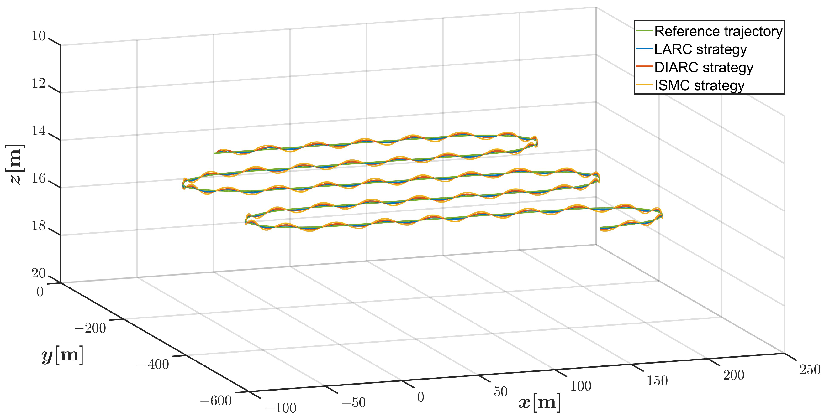
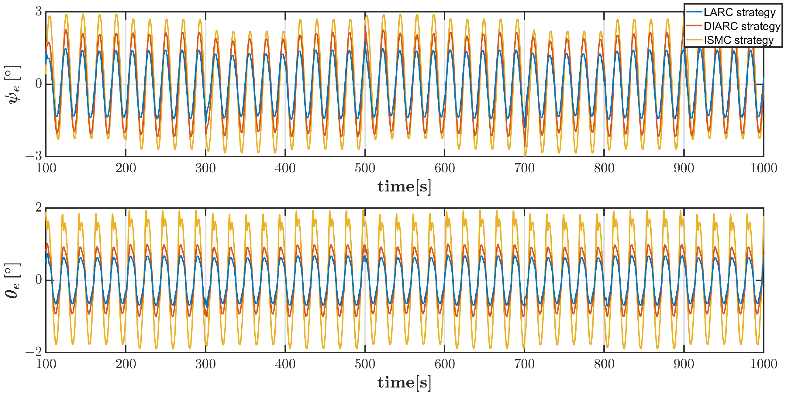
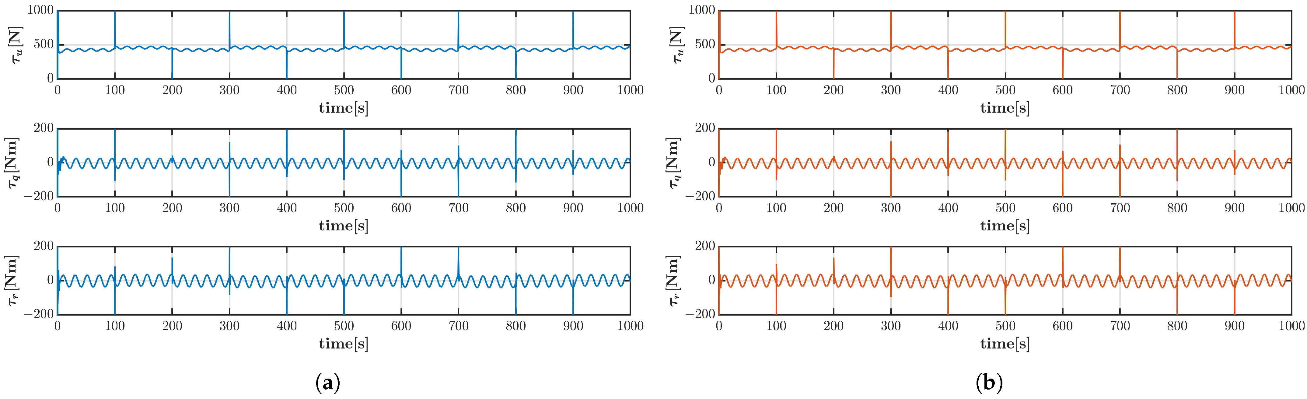
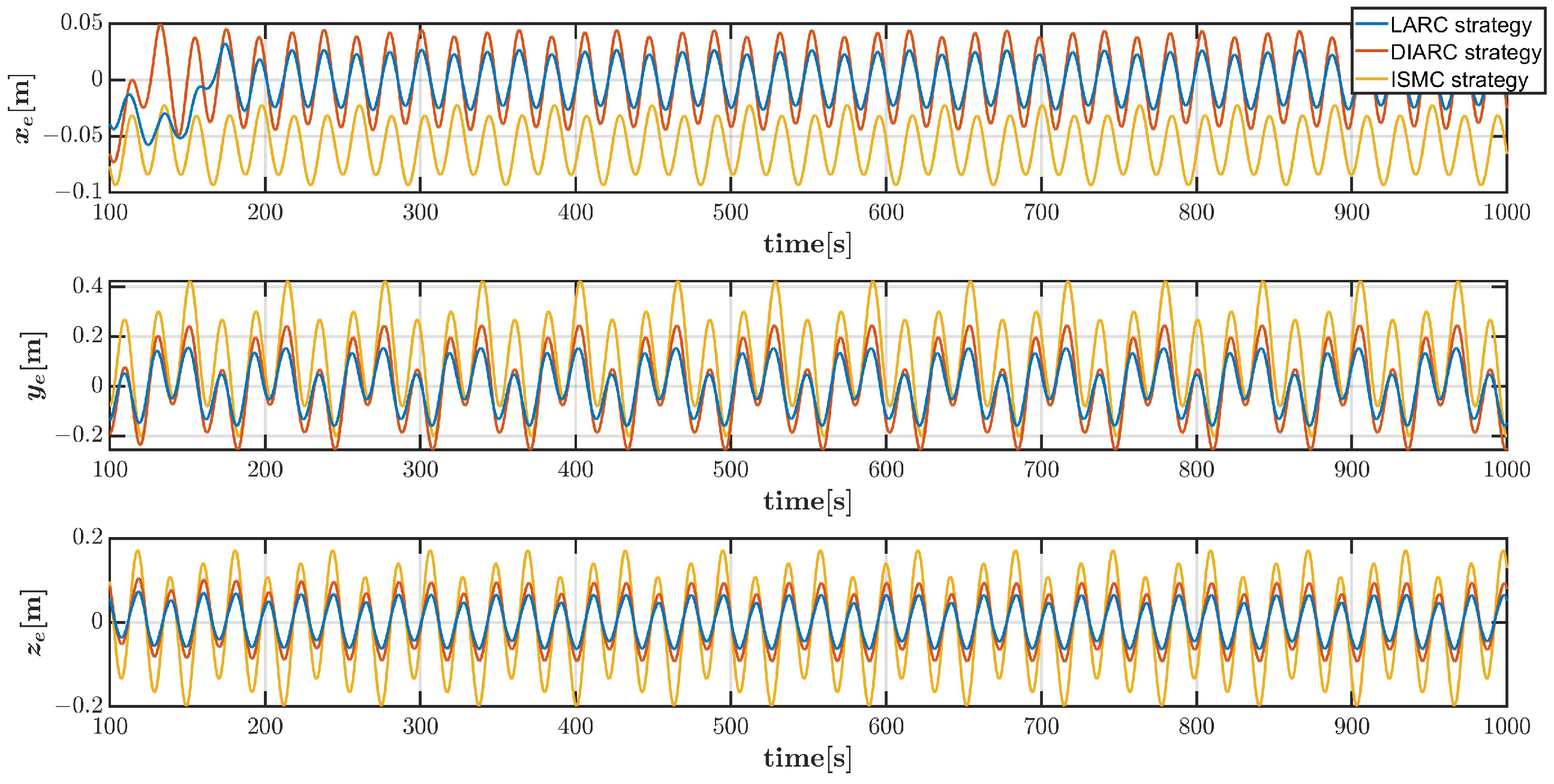
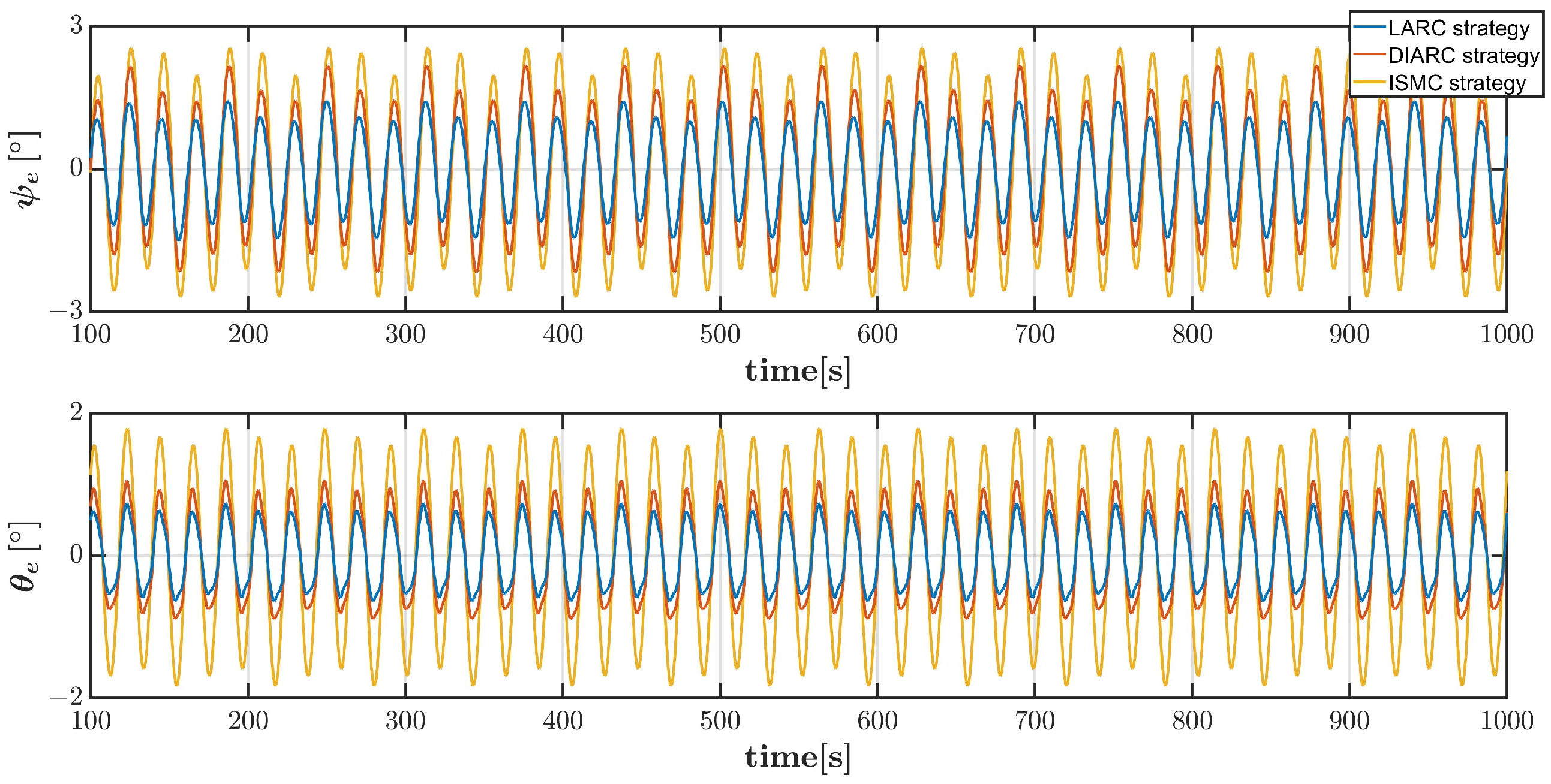
4.1. Combined Reference Trajectory Tracking

The efficacy of the proposed control strategy is initially evaluated through a combined reference trajectory tracking. This trajectory encompasses both linear and curved segments and can be considered for underwater inspection. The details are outlined as follows:

$$\begin{array}{c}{x}_d=\left\{\begin{array}{c}1.5\mathrm{t},0\le \mathrm{t}<100\hfill \\ 50sin\left(0.01\pi \left(\mathrm{t}-100\right)\right)+150,100\le \mathrm{t}<200\hfill \\ -1.5\mathrm{t}+450,200\le \mathrm{t}<300\hfill \\ -50sin\left(0.01\pi \left(\mathrm{t}-300\right)\right),300\le \mathrm{t}<400\hfill \\ 1.5\mathrm{t}-600,400\le \mathrm{t}<500\hfill \\ 50sin\left(0.01\pi \left(\mathrm{t}-500\right)\right)+150,500\le \mathrm{t}<600\hfill \\ -1.5\mathrm{t}+1050,600\le \mathrm{t}<700\hfill \\ -50sin\left(0.01\pi \left(\mathrm{t}-700\right)\right),700\le \mathrm{t}<800\hfill \\ 1.5\mathrm{t}-1200,800\le \mathrm{t}<900\hfill \\ 50sin\left(0.01\pi \left(\mathrm{t}-900\right)\right)+150,900\le \mathrm{t}<1000\hfill \end{array}\right.\hfill \\ y_d=\left\{\begin{array}{c}0,0\le \mathrm{t}<100\hfill \\ 50cos\left(0.01\pi \left(\mathrm{t}-100\right)\right)-50,100\le \mathrm{t}<200\hfill \\ -100,200\le \mathrm{t}<300\hfill \\ 50cos\left(0.01\pi \left(\mathrm{t}-300\right)\right)-150,300\le \mathrm{t}<400\hfill \\ -200,400\le \mathrm{t}<500\hfill \\ 50cos\left(0.01\pi \left(\mathrm{t}-500\right)\right)-250,500\le \mathrm{t}<600\hfill \\ -300,600\le \mathrm{t}<700\hfill \\ 50cos\left(0.01\pi \left(\mathrm{t}-700\right)\right)-350,700\le \mathrm{t}<800\hfill \\ -400,800\le \mathrm{t}<900\hfill \\ 50cos\left(0.01\pi \left(\mathrm{t}-900\right)\right)-450,900\le \mathrm{t}<1000\hfill \end{array}\right.\hfill \\ \hfill z_d=15,0\le \mathrm{t}<1000\hfill \end{array}$$

(33)

The initial conditions of the vehicle are: $x\left(0\right)=1.5$ m, $y\left(0\right)=1$ m, $z\left(0\right)=15$ m, $u\left(0\right)=0.01$ m/s, and $v\left(0\right)=w\left(0\right)=q\left(0\right)=r\left(0\right)=\theta \left(0\right)=\psi \left(0\right)=0$. The number of feedforward compensation iterations is one. In order to verify the control effects under different types of disturbances, two sets of tests with different disturbances are conducted in this scenario, among which Disturbance 1 is related to the velocity and angular velocity states of the vehicle and is time-varying, expressed as:

$$\left\{\begin{array}{c}{D}_u=20sin\left(0.3\mathrm{t}\right)+2cos\left(0.1\mathrm{t}\right)+20u^2+2\mathrm{N}\hfill \\ D_v=15sin\left(0.3\mathrm{t}\right)+1.5cos\left(0.1\mathrm{t}\right)+15v^2+1.5\mathrm{N}\hfill \\ D_w=15sin\left(0.3\mathrm{t}\right)+1.5cos\left(0.1\mathrm{t}\right)+15w^2+1.5\mathrm{N}\hfill \\ D_q=30cos\left(0.3\mathrm{t}\right)+6sin\left(0.1\mathrm{t}\right)+30q^2+6\mathrm{Nm}\hfill \\ D_r=30cos\left(0.3\mathrm{t}\right)+6sin\left(0.1\mathrm{t}\right)+30r^2+6\mathrm{Nm}\hfill \end{array}\right.$$

(34)

Disturbance 2 is also time-varying and set as:

$$\left\{\begin{array}{c}{D}_u=m_{11}\left(0.1sin\left(0.3\mathrm{t}\right)+0.01\right)\mathrm{N}\hfill \\ D_v=0.5m_{22}\left(0.1sin\left(0.3\mathrm{t}\right)+0.01\right)\mathrm{N}\hfill \\ D_w=0.5m_{33}\left(0.1sin\left(0.3\mathrm{t}\right)+0.01\right)\mathrm{N}\hfill \\ D_q=4m_{55}\left(0.1cos\left(0.3\mathrm{t}\right)+0.01\right)\mathrm{Nm}\hfill \\ D_r=4m_{66}\left(0.1cos\left(0.3\mathrm{t}\right)+0.01\right)\mathrm{Nm}\hfill \end{array}\right.$$

(35)

The combined reference trajectory tracking performance of the vehicle by three control strategies under Disturbance 1 is shown in Figure 3, which clearly exhibits that the proposed controller can track the underactuated vehicle to the desired trajectory. In order to demonstrate the tracking performance in the steady state more clearly, the position tracking errors and angle tracking errors under Disturbance 1 after 100 s are shown in Figure 4 and Figure 5, respectively. It can be seen that the error fluctuations generated by the LARC strategy are significantly reduced compared to the DIARC strategy and the ISMC strategy. The control inputs generated by the propeller and rudders by the LARC and DIARC strategies under Disturbance 1 are shown in Figure 6. In addition, the tracking performance under Disturbance 2 is shown in Figure 7, and the corresponding position tracking errors and angle tracking errors after 100 s are shown in Figure 8 and Figure 9, respectively, which also show that the LARC strategy has the best control performance, followed by the DIARC strategy, and then the ISMC strategy. Similarly, the control inputs by the LARC and DIARC strategies under Disturbance 2 are shown in Figure 10. The control inputs under both disturbances indicate that although the discontinuity of the trajectory leads to brief saturation limits at some time points, the overall control inputs are within reasonable ranges.

In order to perform a more quantitative analysis, additional evaluations are carried out on the tracking error data across three different control strategies. The Mean Absolute Error (MAE) and Mean Square Error (MSE) are chosen as the criteria for data assessment, which are widely accepted standards for evaluating tracking errors. The detailed data analysis results under Disturbances 1 and 2 are shown in

Table 1. Performance indices for three control strategies in combined trajectory scenario under system parameter inaccuracies and Disturbance 1.

Performance Indices	LARC	DIARC	ISMC
Total MAE	1.4208	2.0879	3.0263
Total MSE	1.2513	2.5514	4.7696
MAE $\left(x_e\right)$	0.0209	0.0299	0.0536
MSE $\left(x_e\right)$	0.0021	0.0024	0.0045
MAE $\left(y_e\right)$	0.0824	0.1232	0.1715
MSE $\left(y_e\right)$	0.0117	0.0235	0.0461
MAE $\left(z_e\right)$	0.0371	0.0534	0.0995
MSE $\left(z_e\right)$	0.0018	0.0036	0.0126
MAE $\left({\psi }_e\right)$	0.8522	1.2666	1.6016
MSE $\left({\psi }_e\right)$	1.0073	2.0605	3.2048
MAE $\left({\theta }_e\right)$	0.4282	0.6148	1.1001
MSE $\left({\theta }_e\right)$	0.2285	0.4614	1.5015

and

Table 2. Performance indices for three control strategies in combined trajectory scenario under system parameter inaccuracies and Disturbance 2.

Performance Indices	LARC	DIARC	ISMC
Total MAE	1.5013	2.2084	3.4047
Total MSE	1.3958	2.8627	5.4221
MAE $\left(x_e\right)$	0.0214	0.0312	0.2671
MSE $\left(x_e\right)$	0.0020	0.0024	0.0729
MAE $\left(y_e\right)$	0.0833	0.1236	0.1581
MSE $\left(y_e\right)$	0.0110	0.0215	0.0348
MAE $\left(z_e\right)$	0.0382	0.0550	0.1029
MSE $\left(z_e\right)$	0.0018	0.0038	0.0133
MAE $\left({\psi }_e\right)$	0.9137	1.3599	1.6988
MSE $\left({\psi }_e\right)$	1.1365	2.3395	3.6014
MAE $\left({\theta }_e\right)$	0.4447	0.6388	1.1779
MSE $\left({\theta }_e\right)$	0.2444	0.4954	1.6998

, respectively. It can be seen that the control accuracy of the LARC strategy is optimal in all x, y, and z spatial directions, as well as in both pitch and yaw angles. In this scenario, the total MAE created by the LARC strategy is lower than 70% of that of the DIARC strategy and lower than 50% of that of the ISMC strategy, and the corresponding total MSE is lower than 50% of that of the DIARC strategy and lower than 30% of that of the ISMC strategy.

In the LARC strategy, the feedforward compensation ILC part is designed to adjust the optimal reference, which can compensate unmodeled uncertainties to attenuate the tracking error. The projection-type adaptation law with least squares parameter estimation can reduce the tracking errors caused by the uncertainty of system parameters. The nonlinear robust feedback and fast dynamic compensation terms can deal with the nonlinear complex external disturbances and internal uncertainties. Generally, it can be concluded from the above results and analyses that the proposed LARC strategy possesses a high control accuracy and robustness ability for 3D spatial trajectory tracking of an underactuated AUV, and can well meet the high requirements of control performance in repetitive tasks.

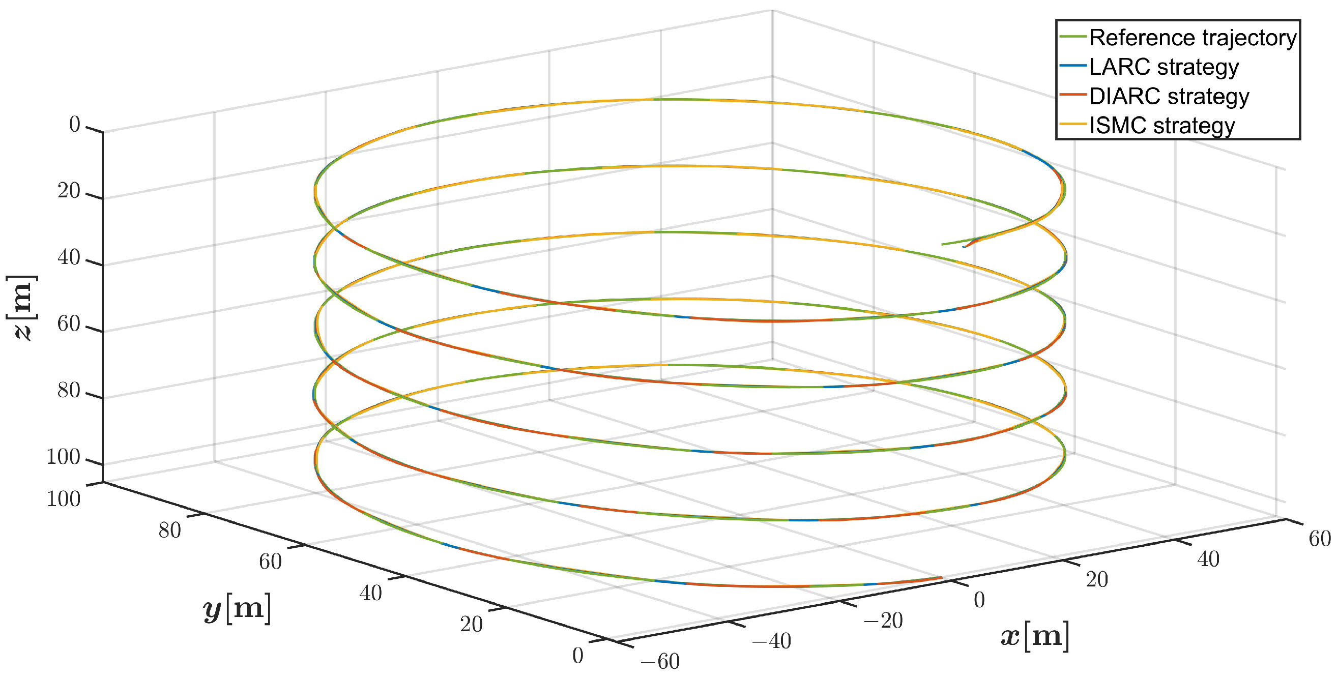
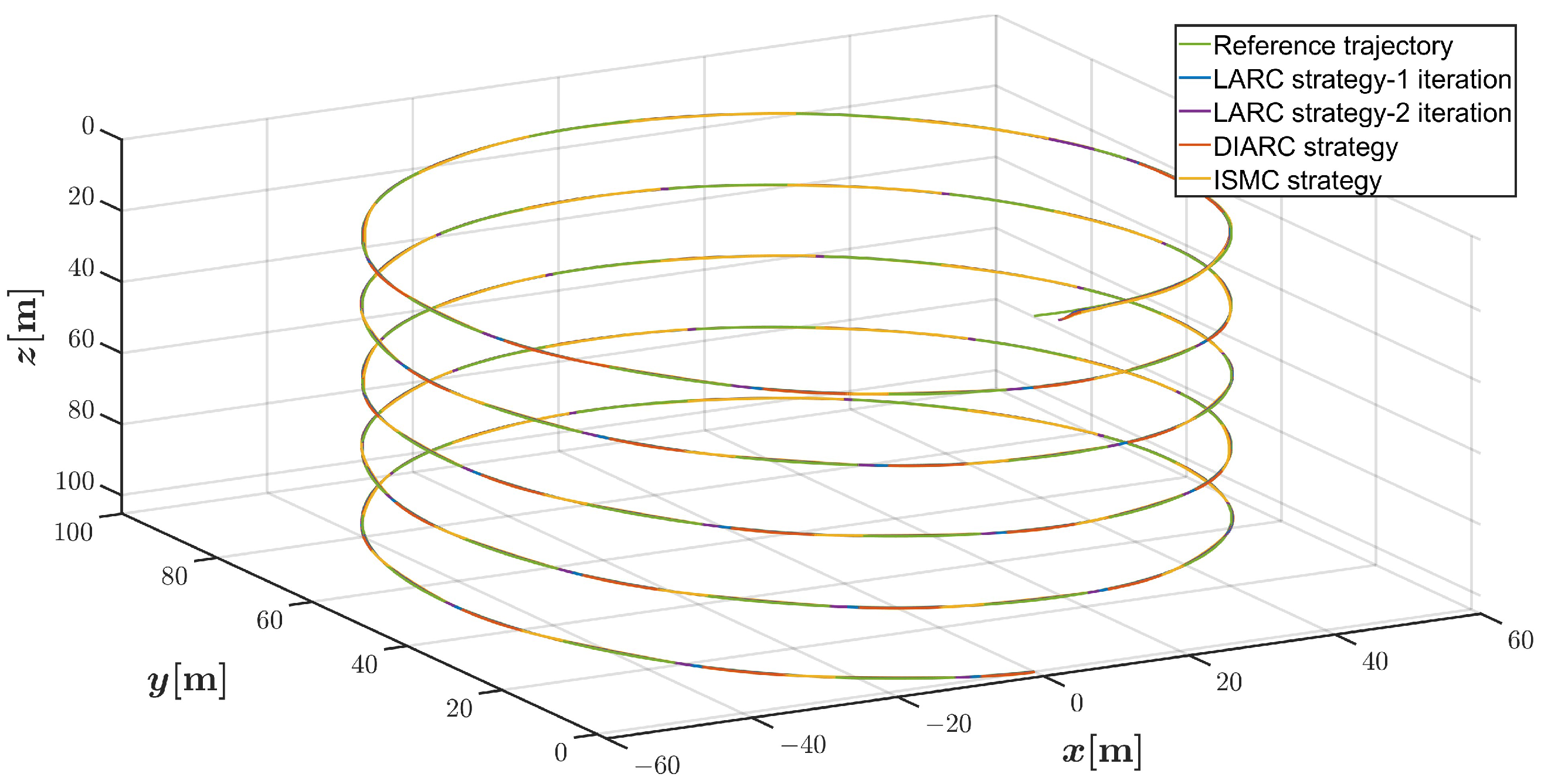
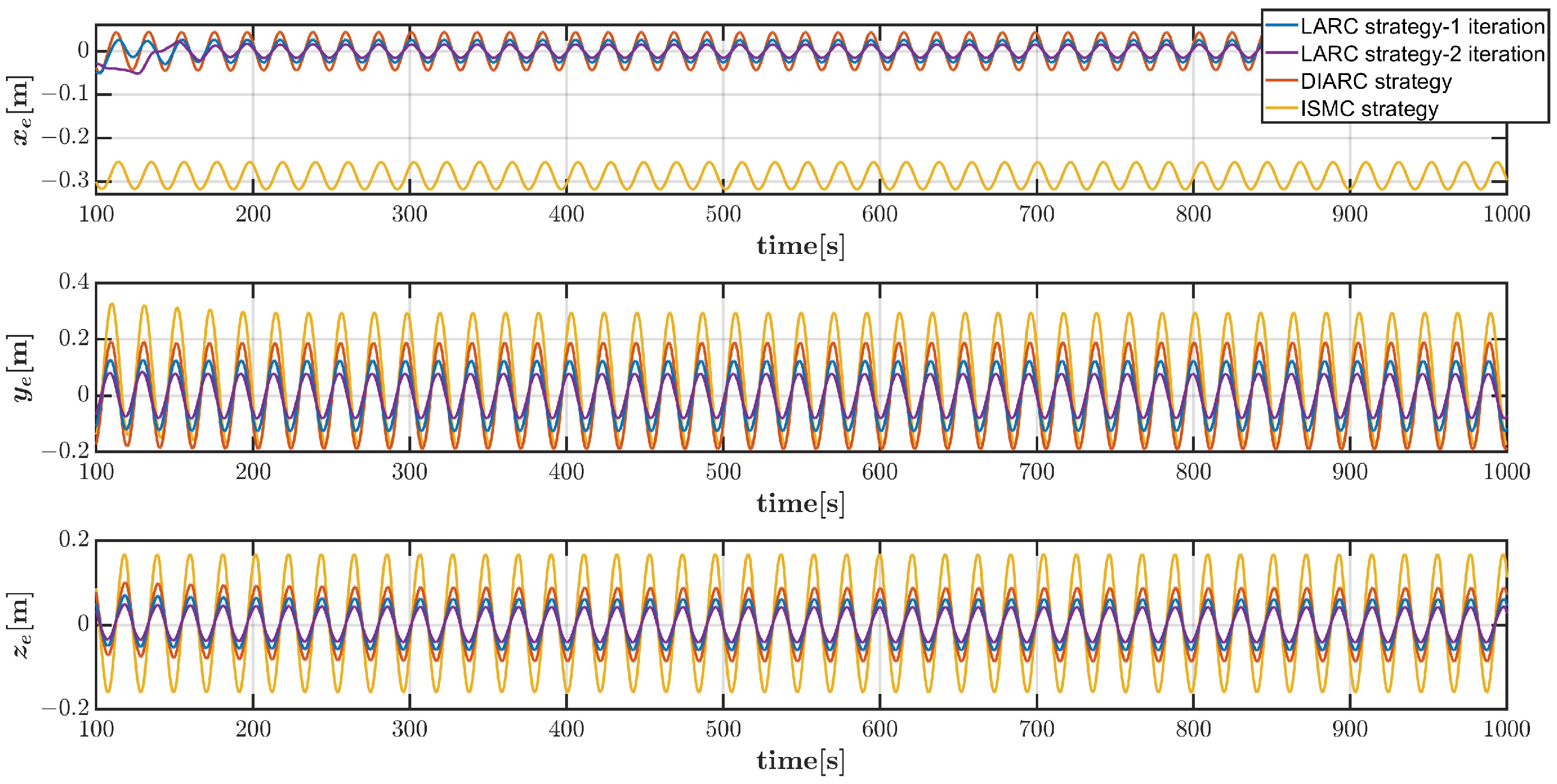
4.2. Helical Dive Reference Trajectory Tracking

The second scenario is the 3D spatial helical dive reference trajectory, which is also a trajectory often used for verification. It can be described as:

$$\left\{\begin{array}{c}{x}_d=50sin\left(0.01\pi t\right)\hfill \\ y_d=-50cos\left(0.01\pi t\right)+50\hfill \\ z_d=0.1t+5\hfill \end{array}\right.$$

(36)

The initial conditions of the vehicle are: $x\left(0\right)=2$ m, $y\left(0\right)=-2$ m, $z\left(0\right)=5.5$ m, $u\left(0\right)=0.01$ m/s, and $v\left(0\right)=w\left(0\right)=q\left(0\right)=r\left(0\right)=\theta \left(0\right)=\psi \left(0\right)=0$. Similarly, in order to verify the control effects under different disturbances, tests are carried out under the same Disturbances 1 and 2 as the combined reference trajectory. Additionally, to visually and quantitatively verify the learning ability of the proposed LARC strategy, when conducting the Disturbance 2 case in this scenario, simulations under the one and two iterations of LARC are carried out.

Figure 11 presents the spatial trajectory tracking performance in the helical dive scenario under Disturbance 1, which illustrates that the proposed controller effectively guides the vehicle along the desired trajectory. The 3D positions and pitch and yaw angles tracking errors after 100 s under Disturbance 1 are exhibited in Figure 12 and Figure 13, respectively. It can be seen that the vehicle controlled by the LARC strategy produces minimal positions and angle fluctuations. Figure 14 displays the control inputs for the LARC and DIARC strategies under Disturbance 1, which exhibits that the control inputs are within the reasonable limits. Accordingly, the spatial tracking performance, 3D positions and angles tracking errors, and control inputs are shown in Figure 15, Figure 16, Figure 17 and Figure 18. The results exhibit that the control error variations by the LARC strategy is still the best under Disturbance 2 in this scenario, and the control inputs are also within the appropriate ranges.

Furthermore, to quantitatively illustrate the effectiveness and robustness of the proposed control strategy in the helical dive scenario, data analyses are conducted utilizing the same evaluation criteria of MAE and MSE.

Table 3. Performance indices for three control strategies in helical dive trajectory scenario under system parameter inaccuracies and Disturbance 1.

Performance Indices	LARC	DIARC	ISMC
Total MAE	1.4609	2.0931	3.0078
Total MSE	2.5752	3.4832	5.2508
MAE $\left(x_e\right)$	0.0232	0.0328	0.0654
MSE $\left(x_e\right)$	0.0044	0.0047	0.0081
MAE $\left(y_e\right)$	0.0879	0.1296	0.1753
MSE $\left(y_e\right)$	0.0199	0.0332	0.0548
MAE $\left(z_e\right)$	0.0379	0.0538	0.0994
MSE $\left(z_e\right)$	0.0021	0.0039	0.0127
MAE $\left({\psi }_e\right)$	0.8517	1.2420	1.5823
MSE $\left({\psi }_e\right)$	1.8165	2.5747	3.6042
MAE $\left({\theta }_e\right)$	0.4602	0.6349	1.0855
MSE $\left({\theta }_e\right)$	0.7324	0.8667	1.5710

and

Table 4. Performance indices in helical dive trajectory scenario under system parameter inaccuracies and Disturbance 2.

Performance Indices	LARC-2 Iteration	LARC-1 Iteration	DIARC	ISMC
Total MAE	1.0766	1.5504	2.2279	3.3942
Total MSE	2.3505	2.6816	3.7884	5.8889
MAE $\left(x_e\right)$	0.0174	0.0234	0.0338	0.2883
MSE $\left(x_e\right)$	0.0041	0.0042	0.0046	0.0855
MAE $\left(y_e\right)$	0.0597	0.0897	0.1316	0.1661
MSE $\left(y_e\right)$	0.0136	0.0197	0.0318	0.0466
MAE $\left(z_e\right)$	0.0280	0.0393	0.0558	0.1026
MSE $\left(z_e\right)$	0.0013	0.0022	0.0041	0.0132
MAE $\left({\psi }_e\right)$	0.6178	0.9214	1.3495	1.6781
MSE $\left({\psi }_e\right)$	1.6288	1.9145	2.8622	3.9934
MAE $\left({\theta }_e\right)$	0.3537	0.4765	0.6571	1.1591
MSE $\left({\theta }_e\right)$	0.7028	0.7411	0.8858	1.7502

demonstrate the detailed performance indices across three control strategies under Disturbances 1 and 2, respectively, which present that the LARC strategy realizes the highest control accuracy across the x, y, and z directions, as well as in the pitch and yaw angles, followed by the DIARC, and then the ISMC. The total MAE produced by the LARC strategy with one iteration is less than 70% of that of the DIARC strategy and less than 50% of that of the ISMC strategy, and the corresponding total MSE is less than 75% of that of the DIARC strategy and less than 50% of that of the ISMC strategy.

In the part of dynamics control, the system parameters of the AUV are often difficult to obtain precisely. The adjustable model compensation term can reduce the tracking error caused by inaccurate parameters to a certain extent. Meanwhile, the AUV is confronted with complex time-varying external disturbances. The nonlinear robust feedback term and fast dynamic compensation term in the proposed control strategy have a good inhibitory effect on the disturbances. Therefore, it can be seen from the above simulation results that the control accuracy of DIARC is superior to that of ISMC. In the part of kinematics control, the ILC feedforward compensation can further reduce the tracking error. Moreover, it can be seen from the Disturbance 2 case of the helical dive trajectory scenario that the LARC strategy iterated twice has a smaller tracking error than the LARC strategy iterated once. This vividly and quantitatively verifies the learning ability of the proposed strategy. From the perspective of computational complexity, the LARC strategy employs an offline learning approach, which eliminates the need for online learning. As a result, the system does not consume online computing resources nor experience failures caused by complex online computations during the AUV trajectory tracking process. This characteristic is beneficial for practical applications. Although the LARC strategy requires offline learning compared with the other control strategies, it is still attractive for significantly improving the control accuracy and robustness of commonly used repetitive tasks. Based on the above simulation results and analyses, the proposed LARC strategy offers significant advantages and options for control methods.

5. Conclusions

In this paper, the LARC strategy was introduced to solve the 3D spatial trajectory tracking control problem of an underactuated AUV in the presence of system parameter uncertainties and complex external disturbances. In the design of the kinematics controller, the serial ILC without requiring an accurate system model was utilized for feedforward compensation to obtain the adjusted desired trajectory, and then the trajectory tracking error dynamics model with ILC trajectory compensation was acquired. Subsequently, the corresponding feedforward-based kinematics controller was introduced and its stability was proved according to Lyapunov’s theorem. In the design of the dynamics controller, the control law is composed of a linear feedback term, a nonlinear robust feedback term, an adjustable model compensation term, and a fast dynamic compensation term, and the projection-type adaptive law was integrated in the control law. According to this control framework, the surge velocity tracking controller, pitch angular velocity tracking controller, and yaw angular velocity tracking controller were designed. The comprehensive simulation study was carried out under different types of disturbances in two scenarios, which showed that the proposed LARC strategy for the underactuated AUV can accurately regulate the vehicle to the predefined trajectory. Quantitative analyses revealed that the MAE and MSE values of the LARC strategy are significantly lower compared to both the DIARC strategy and the ISMC strategy, which greatly improves the trajectory tracking performance and can better meet the high requirements of trajectory tracking accuracy and robustness of repetitive tasks. The results illustrate the effectiveness and advantages of the proposed control strategy. In the future, extending the asymptotic convergence of the controller to fixed-time convergence will be an attractive research direction, and extending this control strategy to the collective behaviors of mobile robots has good research and engineering value.

References

1. Ning, B.; Han, Q.L.; Zuo, Z.; Jin, J.; Zheng, J. Collective behaviors of mobile robots beyond the nearest neighbor rules with switching topology. IEEE Trans. Cybern. 2017, 48, 1577–1590. [Google Scholar] [CrossRef] [PubMed]
2. Li, D.; Du, L. Auv trajectory tracking models and control strategies: A review. J. Mar. Sci. Eng. 2021, 9, 1020. [Google Scholar] [CrossRef]
3. Jawhar, I.; Mohamed, N.; Al-Jaroodi, J.; Zhang, S. An architecture for using autonomous underwater vehicles in wireless sensor networks for underwater pipeline monitoring. IEEE Trans. Ind. Inform. 2018, 15, 1329–1340. [Google Scholar] [CrossRef]
4. Degorre, L.; Fossen, T.I.; Chocron, O.; Delaleau, E. A model-based kinematic guidance method for control of underactuated autonomous underwater vehicles. Control Eng. Pract. 2024, 152, 106068. [Google Scholar] [CrossRef]
5. Zhang, Z.; Lin, M.; Li, D. A double-loop control framework for AUV trajectory tracking under model parameters uncertainties and time-varying currents. Ocean Eng. 2022, 265, 112566. [Google Scholar] [CrossRef]
6. Er, M.J.; Gong, H.; Liu, Y.; Liu, T. Intelligent trajectory tracking and formation control of underactuated autonomous underwater vehicles: A critical review. IEEE Trans. Syst. Man Cybern. Syst. 2023, 54, 543–555. [Google Scholar] [CrossRef]
7. Jalving, B. The NDRE-AUV flight control system. IEEE J. Ocean. Eng. 1994, 19, 497–501. [Google Scholar] [CrossRef]
8. Patil, P.V.; Khan, M.K.; Korulla, M.; Nagarajan, V.; Sha, O.P. Design optimization of an AUV for performing depth control maneuver. Ocean Eng. 2022, 266, 112929. [Google Scholar] [CrossRef]
9. Elmokadem, T.; Zribi, M.; Youcef-Toumi, K. Terminal sliding mode control for the trajectory tracking of underactuated Autonomous Underwater Vehicles. Ocean Eng. 2017, 129, 613–625. [Google Scholar] [CrossRef]
10. Xia, Y.; Huang, Z.; Xu, K.; Xu, G.; Li, Y. Three-Dimensional Trajectory Tracking for a Heterogeneous XAUV via Finite-Time Robust Nonlinear Control and Optimal Rudder Allocation. J. Mar. Sci. Eng. 2022, 10, 1297. [Google Scholar] [CrossRef]
11. Rezazadegan, F.; Shojaei, K.; Sheikholeslam, F.; Chatraei, A. A novel approach to 6-DOF adaptive trajectory tracking control of an AUV in the presence of parameter uncertainties. Ocean Eng. 2015, 107, 246–258. [Google Scholar] [CrossRef]
12. Guerrero, J.; Torres, J.; Creuze, V.; Chemori, A. Trajectory tracking for autonomous underwater vehicle: An adaptive approach. Ocean Eng. 2019, 172, 511–522. [Google Scholar] [CrossRef]
13. Mahapatra, S.; Subudhi, B.; Rout, R.; Kumar, B.K. Nonlinear H∞ control for an autonomous underwater vehicle in the vertical plane. IFAC-PapersOnLine 2016, 49, 391–395. [Google Scholar] [CrossRef]
14. Lapierre, L.; Jouvencel, B. Robust nonlinear path-following control of an AUV. IEEE J. Ocean. Eng. 2008, 33, 89–102. [Google Scholar] [CrossRef]
15. Shojaei, K. Three-dimensional neural network tracking control of a moving target by underactuated autonomous underwater vehicles. Neural Comput. Appl. 2019, 31, 509–521. [Google Scholar] [CrossRef]
16. Hadi, B.; Khosravi, A.; Sarhadi, P. Deep reinforcement learning for adaptive path planning and control of an autonomous underwater vehicle. Appl. Ocean Res. 2022, 129, 103326. [Google Scholar] [CrossRef]
17. Xu, J.; Wang, M.; Qiao, L. Dynamical sliding mode control for the trajectory tracking of underactuated unmanned underwater vehicles. Ocean Eng. 2015, 105, 54–63. [Google Scholar] [CrossRef]
18. Zhou, J.; Zhao, X.; Chen, T.; Yan, Z.; Yang, Z. Trajectory tracking control of an underactuated AUV based on backstepping sliding mode with state prediction. IEEE Access 2019, 7, 181983–181993. [Google Scholar] [CrossRef]
19. Mahapatra, S.; Subudhi, B. Design of a steering control law for an autonomous underwater vehicle using nonlinear H∞ state feedback technique. Nonlinear Dyn. 2017, 90, 837–854. [Google Scholar] [CrossRef]
20. Zhang, W.; Teng, Y.; Wei, S.; Xiong, H.; Ren, H. The robust H-infinity control of UUV with Riccati equation solution interpolation. Ocean Eng. 2018, 156, 252–262. [Google Scholar] [CrossRef]
21. Luo, W.; Cheng, B. Disturbance suppression and NN compensation based trajectory tracking of underactuated AUV. Ocean Eng. 2023, 288, 116172. [Google Scholar] [CrossRef]
22. Li, Z.; Wang, M.; Ma, G. Adaptive optimal trajectory tracking control of AUVs based on reinforcement learning. ISA Trans. 2023, 137, 122–132. [Google Scholar] [CrossRef] [PubMed]
23. Yao, B.; Tomizuka, M. Adaptive robust control of SISO nonlinear systems in a semi-strict feedback form. Automatica 1997, 33, 893–900. [Google Scholar] [CrossRef]
24. Yao, B. High performance adaptive robust control of nonlinear systems: A general framework and new schemes. In Proceedings of the 36th IEEE Conference on Decision and Control, San Diego, CA, USA, 12 December 1997; IEEE: Piscataway, NJ, USA, 1997; Volume 3, pp. 2489–2494. [Google Scholar]
25. Yao, B.; Jiang, C. Advanced motion control: From classical PID to nonlinear adaptive robust control. In Proceedings of the 2010 11th IEEE International Workshop on Advanced Motion Control (AMC), Nagaoka, Japan, 21–24 March 2010; IEEE: Piscataway, NJ, USA, 2010; pp. 815–829. [Google Scholar]
26. Hu, C.; Yao, B.; Wang, Q. Integrated direct/indirect adaptive robust contouring control of a biaxial gantry with accurate parameter estimations. Automatica 2010, 46, 701–707. [Google Scholar] [CrossRef]
27. Mohanty, A.; Yao, B. Indirect adaptive robust control of hydraulic manipulators with accurate parameter estimates. IEEE Trans. Control Syst. Technol. 2010, 19, 567–575. [Google Scholar] [CrossRef]
28. Yao, B. Integrated direct/indirect adaptive robust control of SISO nonlinear systems in semi-strict feedback form. In Proceedings of the Proceedings of the 2003 American Control Conference, Denver, CO, USA, 4–6 June 2003; IEEE: Piscataway, NJ, USA, 2003; Volume 4, pp. 3020–3025. [Google Scholar]
29. Ahn, H.S.; Chen, Y.; Moore, K.L. Iterative learning control: Brief survey and categorization. IEEE Trans. Syst. Man Cybern. Part C (Appl. Rev.) 2007, 37, 1099–1121. [Google Scholar] [CrossRef]
30. Hu, C.; Hu, Z.; Zhu, Y.; Wang, Z.; He, S. Model-data driven learning adaptive robust control of precision mechatronic motion systems with comparative experiments. IEEE Access 2018, 6, 78286–78296. [Google Scholar] [CrossRef]
31. Bristow, D.A.; Tharayil, M.; Alleyne, A.G. A survey of iterative learning control. IEEE Control Syst. Mag. 2006, 26, 96–114. [Google Scholar]
32. Saab, S.S.; Shen, D.; Orabi, M.; Kors, D.; Jaafar, R.H. Iterative learning control: Practical implementation and automation. IEEE Trans. Ind. Electron. 2021, 69, 1858–1866. [Google Scholar] [CrossRef]
33. Fossen, T.I. Handbook of Marine Craft Hydrodynamics and Motion Control; John Willy & Sons Ltd: Hoboken, NJ, USA, 2011. [Google Scholar]
34. Guo, C.; Han, Y.; Yu, H.; Qin, J. Spatial path-following control of underactuated auv with multiple uncertainties and input saturation. IEEE Access 2019, 7, 98014–98022. [Google Scholar] [CrossRef]
35. Breivik, M.; Fossen, T.I. Guidance-based path following for autonomous underwater vehicles. In Proceedings of the OCEANS 2005 MTS/IEEE, Washington, DC, USA, 17–23 September 2005; IEEE: Piscataway, NJ, USA, 2005; pp. 2807–2814. [Google Scholar]
36. Huang, Z.; Xia, Y.; Wang, W.; Xu, G.; Xiang, X.; Xu, K. SHSA-based adaptive roll-safety 3D tracking control of a X-Rudder AUV with actuator dynamics. Ocean Eng. 2022, 265, 112544. [Google Scholar] [CrossRef]
37. Goodwin, G.C.; Mayne, D.Q. A parameter estimation perspective of continuous time model reference adaptive control. Automatica 1987, 23, 57–70. [Google Scholar] [CrossRef]
38. Yao, B.; Palmer, A. Indirect adaptive robust control of SISO nonlinear systems in semi-strict feedback forms. IFAC Proc. Vol. 2002, 35, 397–402. [Google Scholar] [CrossRef]
39. Landau, I.D.; Lozano, R.; M’Saad, M.; Karimi, A. Adaptive Control: Algorithms, Analysis and Applications; Springer Science & Business Media: Berlin/Heidelberg, Germany, 2011. [Google Scholar]
40. Pettersen, K.Y.; Egeland, O. Time-varying exponential stabilization of the position and attitude of an underactuated autonomous underwater vehicle. IEEE Trans. Autom. Control 1999, 44, 112–115. [Google Scholar] [CrossRef]
Figure 1. Spatial trajectory tracking schematic diagram of an AUV.
Jmse 13 01151 g001
Figure 2. Schematic diagram of the proposed LARC strategy for the underactuated AUV.
Jmse 13 01151 g002
Figure 3. Trajectory tracking results in combined trajectory scenario by three control strategies under system parameter inaccuracies and Disturbance 1.
Jmse 13 01151 g003
Figure 4. Vehicle position tracking errors in combined trajectory scenario by three control strategies under system parameter inaccuracies and Disturbance 1.
Jmse 13 01151 g004
Figure 5. Vehicle angle errors in combined trajectory scenario by three control strategies under system parameter inaccuracies and Disturbance 1.
Jmse 13 01151 g005
Figure 6. Control inputs of the vehicle by (a) LARC strategy and (b) DIARC strategy in combined trajectory scenario under system parameter inaccuracies and Disturbance 1.
Jmse 13 01151 g006
Figure 7. Trajectory tracking results in combined trajectory scenario by three control strategies under system parameter inaccuracies and Disturbance 2.
Jmse 13 01151 g007
Figure 8. Vehicle position tracking errors in combined trajectory scenario by three control strategies under system parameter inaccuracies and Disturbance 2.
Jmse 13 01151 g008
Figure 9. Vehicle angle errors in combined trajectory scenario by three control strategies under system parameter inaccuracies and Disturbance 2.
Jmse 13 01151 g009
Figure 10. Control inputs of the vehicle by (a) LARC strategy and (b) DIARC strategy in combined trajectory scenario under system parameter inaccuracies and Disturbance 2.
Jmse 13 01151 g010
Figure 11. Trajectory tracking results in helical dive trajectory scenario by three control strategies under system parameter inaccuracies and Disturbance 1.
Jmse 13 01151 g011
Figure 12. Vehicle position tracking errors in helical dive trajectory scenario by three control strategies under system parameter inaccuracies and Disturbance 1.
Jmse 13 01151 g012
Figure 13. Vehicle angle errors in helical dive trajectory scenario by three control strategies under system parameter inaccuracies and Disturbance 1.
Jmse 13 01151 g013
Figure 14. Control inputs of the vehicle by (a) LARC strategy and (b) DIARC strategy in helical dive trajectory scenario under system parameter inaccuracies and Disturbance 1.
Jmse 13 01151 g014
Figure 15. Trajectory tracking results in helical dive trajectory scenario under system parameter inaccuracies and Disturbance 2.
Jmse 13 01151 g015
Figure 16. Vehicle position tracking errors in helical dive trajectory scenario under system parameter inaccuracies and Disturbance 2.
Jmse 13 01151 g016
Figure 17. Vehicle angle errors in helical dive trajectory scenario under system parameter inaccuracies and Disturbance 2.
Jmse 13 01151 g017
Figure 18. Control inputs of the vehicle by (a) LARC-one iteration and (b) LARC-two iteration in helical dive trajectory scenario under system parameter inaccuracies and Disturbance 2.
Jmse 13 01151 g018