Article

Adaptive Convolution Kernels Construction Based on Unsupervised Learning for Underwater Acoustic Detection

1
State Key Laboratory of Acoustics, Institute of Acoustics, Chinese Academy of Sciences, Beijing 100190, China
2
University of Chinese Academy of Sciences, Beijing 101408, China
*
Author to whom correspondence should be addressed.
J. Mar. Sci. Eng. 2025, 13(6), 1136; https://doi.org/10.3390/jmse13061136
Submission received: 24 April 2025 / Revised: 25 May 2025 / Accepted: 29 May 2025 / Published: 6 June 2025
(This article belongs to the Section Ocean Engineering)

Abstract

:
In the field of Direction of Arrival (DOA) estimation, due to the complexity of ocean noise and the limitations of using array apertures, the bearing time record (BTR) obtained by CBF typically exhibits low signal-to-noise ratio (SNR) and wide mainlobe width. To address this issue, we propose an adaptive 2D convolution kernel construction method that utilizes an improved k-means clustering algorithm to extract adaptive mainlobe visual patterns from historical BTR data as convolution kernels. Experimental results show that our method can effectively reduce noise levels within multiple target environments.

1. Introduction

In underwater passive detection, the bearing time record (BTR), which is a visual tool for tracking the trajectory of underwater targets, plays a crucial role. BTRs are created by plotting the power of beamforming signals using beamforming algorithms like Conventional Beamforming (CBF) or Minimum Variance Distortionless Response (MVDR) over a two-dimensional (2D) plane of time and bearing angle [1,2]. In a BTR, the horizontal axis represents the bearing angle, while the vertical axis represents time. High-intensity regions correspond to strong signal returns from specific directions at particular times, indicating the presence and movement of targets, which can complete the task of target detection and tracking. The primary goal of underwater passive detection is to enhance the capability of detecting weak targets, with the expansion of the detection range being a key pursuit. Long-range detection performance is typically reflected in the identification of low-intensity signals in the BTR. An effective strategy for optimizing the design of acoustic arrays is to increase the number of array elements N while maintaining a constant array aperture L = N d , thereby improving resolution and array gain. According to the classical array gain formula, the theoretical gain is given by AG = 10 log 10 ( N ) [3]. However, indiscriminately increasing the number of elements can result in an excessively long array, raising system design and deployment costs. Additionally, if the element spacing d becomes too small, the assumption of noise orthogonality, E [ n i n j * ] = 0 ( i j ) , may no longer hold, which would degrade the actual array gain and compromise detection performance [4]. Ref. [5] emphasized that effective separation of signal and noise spaces is essential for achieving optimal array gain. Therefore, array design must strike a balance between gain improvement, cost efficiency, and practical deployment to ensure overall system performance.
To reduce noise on the BTR, enhance the visibility of weak targets, and improve feature detectability, image processing techniques have been widely used in passive sonar post-processing for many years. Currently, popular image-denoising methods can be roughly classified into two categories: smoothing filter-based methods and block-based methods. In image processing, convolution operations are commonly employed for image filtering. By convolving an image with a kernel (or filter), the pixel values of the image are adjusted according to the weights of its neighboring pixels, resulting in noise reduction, edge detection, and feature enhancement. Commonly used image kernels include Gaussian filters, mean filters, and median filters [6]. Li et al. [7] proposed a method for processing non-uniform, non-stationary BTR images with noisy backgrounds by combining the median filter and sorted truncated mean for background balancing. However, all of these balancing methods are based on smoothing operations around the image areas, which will cause blurry details and information loss, especially in complex images containing more details. However, these methods are based on the smoothing operation applied to the peripheral areas of the image, which can lead to blurred details and loss of information, especially in complex images containing more detailed features.
The second method is a block-based approach, where the image is divided into blocks according to preset standards. Blocks with smoother textures are selected for matching. Ref. [8] introduced the K-SVD algorithm, which uses an overcomplete dictionary to achieve sparse representation for signal and image compression and denoising. Ref. [9] proposed the NLM (Non-Local Means) algorithm, which leverages non-local information within images to improve denoising while preserving details and texture information. Refs. [10,11] introduced a 3D block matching method (BM3D) that separates noise and signal in higher dimensions, achieving significant feature enhancement. However, all these algorithms require prior estimation of the noise level in the image and are overly dependent on poorly definable preset standards. Ref. [12] proposed a new algorithm framework called Block Matching-Subband Extrema Energy Detection (BM-SEED) for denoising and enhancing the weak targets of BTRs. However, these algorithms require prior estimation of the image noise levels and are heavily reliant on preset standards that are difficult to determine. Ref. [13] proposed a BTR image-denoising method based on principal component analysis (PCA) dimensionality reduction, but this method is unable to effectively enhance weak targets. Referencing [14,
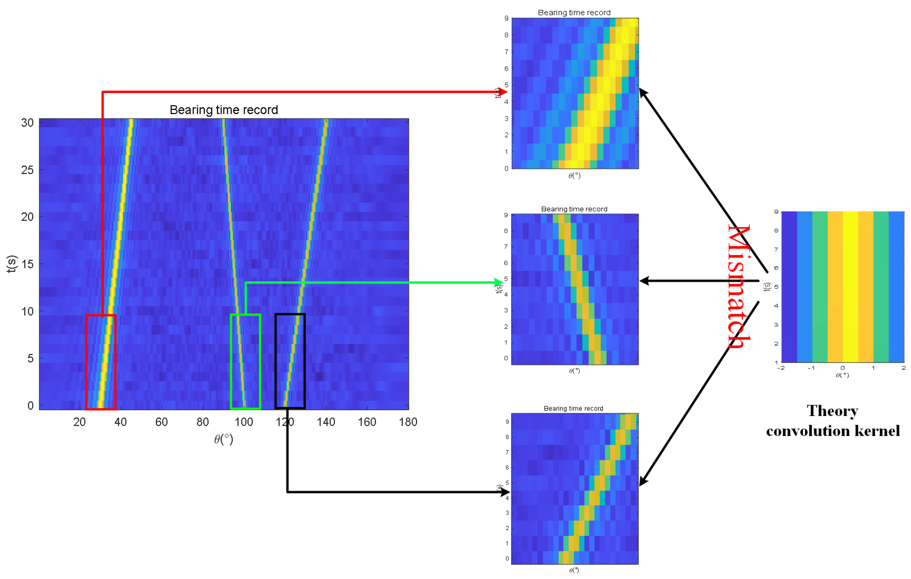
15], a deblurring algorithm is applied to an image via convolution to a uniform linear array (ULA). Deconvolution convention beamforming, which serves as an improved high-resolution algorithm for traditional beamforming, can significantly narrow the main lobe width and reduce the level of side lobes and has been widely used. However, under low signal-to-noise ratio (SNR) conditions, the point spread function (PSF) derived from array information is an idealized, theoretical representation, which may not accurately correspond to the actual noisy beam response. As a result, deconvolution may amplify noise in the original signal due to this mismatch. The BTR is a two-dimensional image, with the horizontal axis representing angles and the vertical axis representing time. Consequently, Ref. [16] proposed extending the one-dimensional PSF into the temporal dimension to develop a 2D PSF with the horizontal axis denoting angles and the vertical axis representing time. This enables 2D deconvolution beamforming to acquire greater temporal gains. However, this approach has disadvantages: when targets undergo high-speed evasive maneuvers, their trajectories may shift in angle. The theoretical 2D PSF, lacking an inherent angular deviation, may not perform adequately if the time window T is insufficient, failing to yield sufficient temporal gain. As a result, its performance may fall short of expectations for ideal temporal gains under rapid maneuvers and could even underperform compared with the CBF algorithm’s beam response.
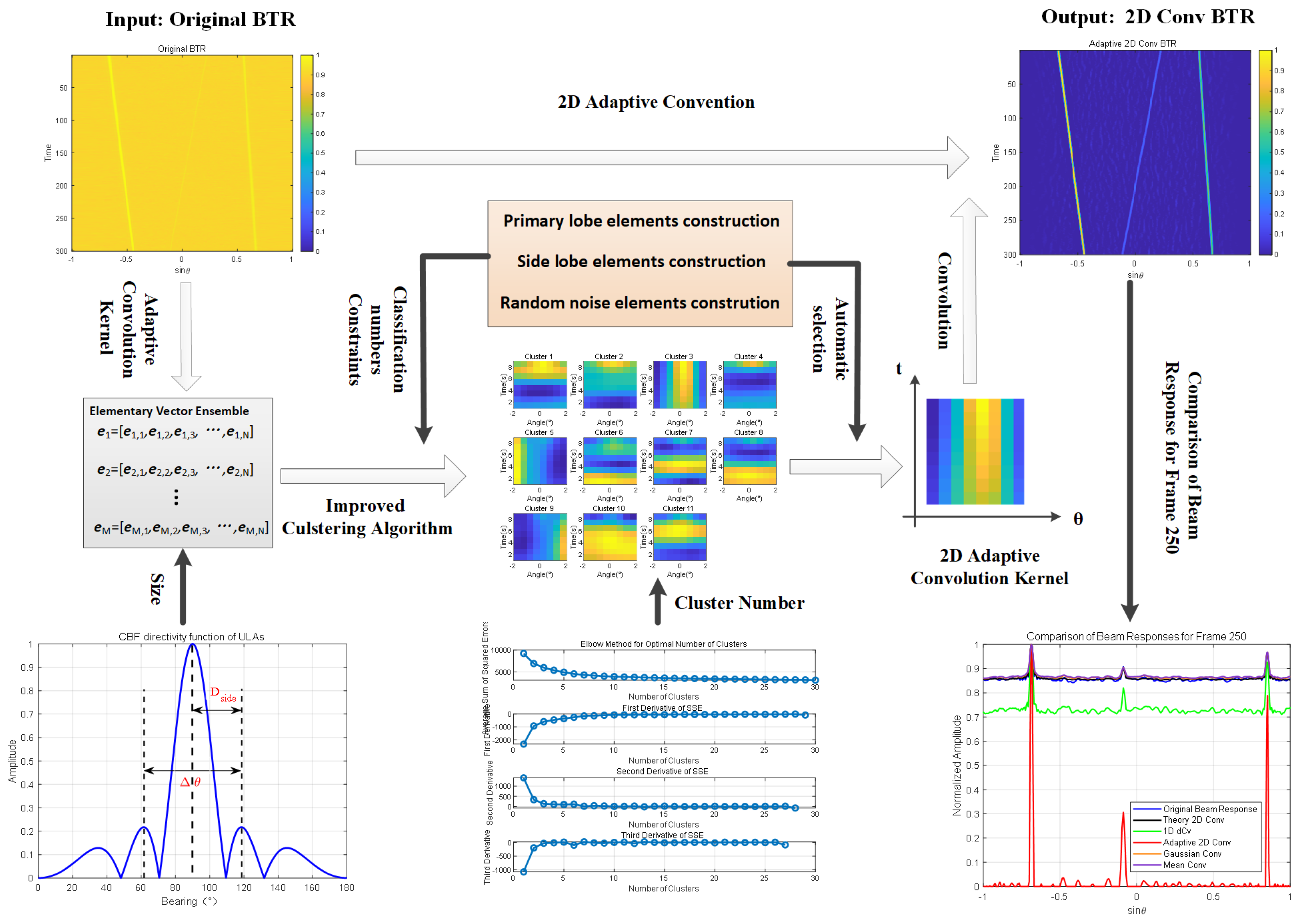
In passive detection, the parameters of the surrounding environment are unknown. To acquire these real-time parameters, we employ an adaptive method to extract the real-time parameters from the BTR. By adopting this approach, we can achieve feature enhancement. The core idea behind this method is to utilize a self-adaptive convolution kernel that matches the stripe pattern present in the current BTR for image processing. In image processing, convolution involves applying a small kernel over local areas of an image to extract features, reduce noise, or achieve other visual effects. The fundamental concept is to replace each pixel in the image with a weighted average value. By selecting appropriate kernel functions, various image processing tasks can be accomplished. Therefore, we construct a visual template representing the main lobe using the K-means algorithm, which serves as our self-adaptive convolution kernel. This approach offers two significant advantages: first, it is an artificial intelligence-based method that maximizes the extraction of real-time parameters from the stripe information on the BTR, avoiding the blind box process; second, it yields a self-adaptive convolution kernel that matches the actual probability statistical characteristics. Experimental results have shown that when compared with convolutional beamforming (CBF), Theory 2D convolution (Theory 2D Conv), 1D deconvolution beamforming (1D dCv), Gaussian convolution (Gaussian Conv), mean convolution (Mean Conv), and median convolution (Median Conv), our proposed Adaptive 2D convolution (adaptive 2D Conv) effectively suppresses background noise and side lobe levels while enhancing weak targets under low SNR conditions and reduces the main lobe width to improve resolution. The remainder of this paper is organized as follows: Section 2 provides a comprehensive review of related work; Section 3 presents the proposed Adaptive 2D Conv in detail; Section 4 and Section 5 analyze the simulation and experiment results, respectively; finally, Section 6 gives the final conclusion of this work.

2. Related Work

The research object of this paper is the BTR, which first receives the noise signal emitted by the ship using a sonar array and estimates the DOA to obtain the spatial spectrum chart. Then, for each snapshot, the spatial spectrum charts are accumulated along the time dimension to form a 2D matrix with the x-coordinate representing the full spatial scale and the y-coordinate representing time. Each pixel point in the matrix only represents the amplitude of the target signal at the current position and time. The visual effect is similar to an image with intersecting trajectories, which can complete the task of target detection and tracking. In recent years, image processing methods have been applied to passive sonar post-processing to reduce background noise levels and improve angular resolution.

2.1. Classical Convolution Kernels for Image Filtering

Convolution operations are commonly used in image processing to filter images. By convolving an image with a kernel (or filter), the pixel values are adjusted according to the weighted average of their neighboring pixels, which results in noise reduction, edge detection, and feature enhancement. Commonly used convolution kernels include Gaussian filters, mean filters, and median filters. However, these methods rely on smoothing operations applied to the surrounding areas of the image, which can blur details and lead to information loss, especially in complex images with intricate features.
Given a BTR matrix B ( θ , t ) of size P × Q and a convolution kernel K ( θ k , t k ) of size p × q , the convolution operation can be expressed as
B ( θ , t ) = ( B K ) ( θ , t ) = θ k = 0 p 1 t k = 0 q 1 B ( θ θ k , t t k ) · K ( θ k , t k )
where i ranges from 0 to p 1 horizontally, and j ranges from 0 to q 1 vertically, representing the position of the convolution kernel K as it slides over the original BTR B. When performing convolution operations, normalization of the kernel K is required to maintain the overall brightness of the image. This ensures that the sum of all elements in K equals 1.

2.1.1. Gaussian Filter

The Gaussian filter uses a 2D Gaussian distribution function to generate the Gaussian kernel K Gaussian . For a Gaussian kernel K Gaussian of size n × n , where n is an odd number, the center position is at n 1 2 , n 1 2 . The weights are calculated using the following formula:
K Gaussian ( θ k , t k ) = 1 2 π σ 2 exp ( θ 2 n 1 2 ) 2 + ( t 2 n 1 2 ) 2 2 σ 2
where σ is the standard deviation of the Gaussian distribution, which controls the degree of smoothing. A larger σ results in more significant smoothing. Gaussian filtering applies a weighted average process to the image, with the central pixel given more weight, which decreases with increasing distance from the center. It effectively suppresses Gaussian noise but is less effective against impulse noise, such as salt-and-pepper noise.

2.1.2. Mean Filter

The mean filter is a linear filtering method that replaces the center pixel with the average value of its neighboring pixels, thus achieving image smoothing and noise reduction. For a mean filter kernel K mean of size p × q , all elements of the kernel are equal, and it can be expressed as
K mean ( θ k , t k ) = 1 p q
For each central pixel, the sum of all neighboring pixels, including itself, is calculated, and the average value is used as the output. Mean filtering is effective for smoothing uniformly distributed noise. However, it is less effective at removing salt-and-pepper noise, as such noise typically appears as isolated extreme points. In this case, the mean filter may spread the noise across the entire neighborhood, potentially degrading image quality.

2.1.3. Median Filter

The median filter is a non-linear filtering method that replaces the center pixel with the median value of its neighboring pixels. It is particularly effective in removing salt-and-pepper noise. For a median filter kernel K median of size p × q , where p and q are typically odd values, let the set of pixel values within the window be denoted as B = { B 1 , B 2 , , B p q } . First, the pixel values are sorted in ascending order, and the middle value is selected as the median filtered pixel value. Median filtering effectively removes salt-and-pepper noise by replacing the central pixel with the median of its neighboring pixels.

2.2. Deconvolved Conventional Beamforming

Ref. [14] introduces a deblurring algorithm for images using convolution, applied to the uniform linear array (ULA), and proposes a CBF method by deconvolution, which utilizes the Richardson–Lucy (R–L) algorithm for iterative solutions based on Bayesian principles [17]. Under the plane wave model, there is only a phase difference between signals received by different array elements due to differences in distance, leading to completely coherent array signals. One primary goal of array signal processing is to suppress incoherent noise through a spatial accumulation process. In deconvolution theory, CBF can be considered as the result of convolving the energy distribution of target sources with the array beam response.
B C B F ( s i n θ ) = 1 1 B p ( s i n θ s i n ϑ ) A ( s i n ϑ ) d s i n ϑ
where s i n ϑ represents the sine value of the incident direction of the target source under far-field conditions, and  s i n θ represents the sine value of the beam response direction. In deconvolution, B p ( θ | ϑ ) is referred to as the PSF, which represents the energy response of the azimuth spectrum to a unit-intensity target at a specific direction ϑ ; obviously, the PSF is determined solely by the array manifold. A ( s i n ϑ ) represents the complete spatial energy distribution of the source signal, which corresponds to the result of DOA estimation, i.e., the estimated beam direction energy. It is known that DOA B C B F ( s i n θ ) can be obtained by deconvolving with the array beam response B p ( s i n θ s i n ϑ ) , which can be calculated using array parameters, and the Bayesian-inspired R–L iterative algorithm is a typical example of spatial deconvolution and has been widely used in this field.
When the observation angle is represented as a sine or cosine value, the PSF in Equation (4) exhibits shift-invariance. Therefore, considering the shift-invariant property of the beam response, it is suggested to convert the horizontal axis of the BTR from linear angular values to their corresponding sine values. This transformation aligns with the directional characteristics of the CBF function, thereby enhancing the accuracy and consistency of directional estimates while preserving the system’s shift invariance.

2.3. Construction of 2D Theory Convolution Kernel

Considering both time and azimuthal information within BTRs, we propose a method to extend the 1D theory convolution kernel K T h e o r y 1 D calculated from array parameters into a 2D theory convolution kernel K T h e o r y 2 D . This extension incorporates the time dimension to achieve greater temporal gain. Assuming K T h e o r y 1 D = B p ( s i n θ s i n ϑ ) , which is calculated from array information, it is typically represented as K T h e o r y 1 D = ( 0 sin θ ) when the incident angle ϑ = 0 ; when extended to a 2D form in the time domain, the resulting kernel is given by Equation (5). However, under high-speed motion conditions, as shown in Figure 1, three targets with varying tilt angles are observed during high-speed maneuvers. Due to the angular changes in the targets during rapid movements, the angle between them is not fixed. The 2D theory convolution kernel K T h e o r y 2 D , extended from one dimension (1D) along the time axis, visually appears as a straight line. As a result, there is a misalignment between the K T h e o r y 2 D and the actual trajectory of the target during high-speed maneuvers. Consequently, the performance of Theory 2D Conv often fails to meet the expected theoretical temporal gain and may even perform worse than the original beam response in practical applications.
K T h e o r y 2 D ( θ k , t k ) = B p ( = sin θ ) B p ( = sin θ ) B p ( = sin θ ) t k = T
To address the limitations of existing methods, we propose an adaptive 2D convolution kernel construction approach, denoted as K A d a p t i v e . By extracting peak values from the BTR and using cluster analysis to identify visual patterns related to the main lobe, side lobes, and random noise, our method dynamically adjusts the convolution kernel construction to achieve lower background noise and higher resolution. The 2D adaptive convolution method (Adaptive 2D Conv) based on the K A d a p t i v e demonstrates significant advantages in low SNR and high-speed target maneuver conditions. It overcomes the limitations of one-dimensional deconvolution beamforming (1D dCv), two-dimensional convolution (Theory 2D Conv), and various smoothing filters (such as Gaussian Conv, Mean Conv, and Median Conv) while significantly improving background noise suppression capability and main lobe resolution. The proposed method achieves three primary objectives: first, it improves detection resolution by narrowing the main lobe width; second, it removes side lobes to reduce false alarms caused by side lobes being misidentified as real targets; and third, it effectively reduces background noise and lowers the chances of background noise being mistaken for real targets.

3. Method

The overall framework of the proposed method is shown in Figure 2. The present work applies to BTR obtained from passive sonar using CBF and proposes an Adaptive 2D Convention (Adaptive 2D Conv) method, which accounts for both time and azimuthal physical dimensions. Initially, the method employs conventional array beamforming for Uniform Linear Arrays (ULA) under the far-field assumption to generate BTR based on time and azimuth. Then, an open peak extraction process is performed on the BTR. During this process, the appropriate element size should be selected based on the directivity function of CBF and the parameters of the receiving array. Subsequently, an enhanced clustering algorithm is employed along with an automatic strategy for determining the number of clusters based on multi-order derivatives of the Sum of Squared Errors (SSE). This approach allows for the extraction of visual templates representing the main lobe, denoted as K A d a p t i v e . Finally, by performing Adaptive 2D Conv between this K A d a p t i v e and BTR, we can obtain the BTR image after convolution. Compared with traditional methods, the proposed method demonstrates better performance.

3.1. 2D Adaptive Convolution Kernel

To construct K A d a p t i v e , we first calculate its size according to the directivity function of CBF in ULA. Then, an improved k-means algorithm is employed to extract the main lobe visual pattern, which serves as K A d a p t i v e .

3.1.1. Size of Adaptive Convolution Kernels

To detect all potential targets in the BTR, we apply an open peak extraction method, where each peak represents valuable physical information. The concept of “element” introduced by [18] is used to construct visual units and establish associations between peaks in the BTR and their underlying physical meanings. It is crucial to select an appropriate element size to avoid misinterpreting isolated, discontinuous, low-intensity noise points as actual targets. In BTRs, target trajectories appear as high-intensity continuous segments, while sidelobes are typically represented by lower but continuous-intensity portions on either side of the main lobe. To minimize interference from the sidelobes and ensure that the main lobe is centered in the visual template, the element width should be set to twice the distance between the main lobe and the first sidelobe.
As shown in Figure 3, to calculate the main-to-sidelobe distance for the CBF method, we identify the position of the maximum value of the first sidelobe. This requires differentiating the directivity function D ( θ ) with respect to θ , neglecting the absolute value and the constant factor A.
d d θ sin ( N π d / λ sin ( θ ) ) N sin ( π d / λ sin ( θ ) ) = π d N cos π N d sin ( θ ) λ sin π N d sin ( θ ) λ tan π d sin ( θ ) λ cos ( θ ) N λ sin π d sin ( θ ) λ
Equation (6) describes the derivative of the directivity function for the CBF algorithm.
The position of the first sidelobe’s maximum value is the first positive root of this equation, which can be solved using specific parameters and numerical methods. The position of the maximum value of the first sidelobe, obtained numerically, is denoted as D s i d e , representing the main-to-sidelobe distance.
The width of element Δ θ is then defined as
Δ θ = 2 D s i d e

3.1.2. Construction of Adaptive Convolution Kernels

The clustering process aims to partition a set of elements { e 1 , e 2 , , e n } into k clusters based on their similarity. The clustering iteration process involves several key steps: element assignment based on correlation coefficients, updating cluster centers, checking for convergence, and finally, outputting the results.
  • Step 1: Element Assignment
Each element e i is assigned to one of the k clusters based on the correlation between the element and the cluster centers. The correlation between an element e i and a cluster center c j ( t ) at iteration t is calculated as
r ( e i , c j ( t ) ) = p = 1 P e i ( p ) c j ( t , p ) p = 1 P ( e i ( p ) ) 2 · p = 1 P ( c j ( t , p ) ) 2 ,
where P is the dimensionality of the elements, and  e i ( p ) and c j ( t , p ) denote the p-th dimension of the element and the cluster center, respectively.
Each element e i is assigned to the cluster j that maximizes the correlation r ( e i , c j ( t ) ) :
y i ( t ) = arg max j r ( e i , c j ( t ) ) ,
where y i ( t ) denotes the cluster label assigned to element e i at iteration t.
  • Step 2: Cluster Center Update
Once all elements are assigned to clusters, the cluster centers are updated based on the mean of the elements in each cluster. The new cluster center c j ( t + 1 ) for cluster j is calculated as:
c j ( t + 1 ) = 1 | S j | i S j e i .
where S j = { i y i ( t ) = j } represents the set of elements assigned to cluster j, and  | S j | is the number of elements in S j .
  • Step 3: Convergence Check
The iteration stops when the cluster centers converge. Convergence is determined by the maximum change in cluster centers between two consecutive iterations:
max j c j ( t + 1 ) c j ( t ) < ε ,
where ε is a small threshold value that defines convergence. If the condition in (10) is not satisfied, the process returns to the element assignment step.
  • Output
Upon convergence, the algorithm outputs the final cluster labels y i ( t ) and cluster centers C ( t ) = { c 1 ( t ) , c 2 ( t ) , , c k ( t ) } .

3.1.3. Automatically Determine the Number of Clusters

Theoretically, the number of visual templates on BTR should correspond to the main lobe V m a i n , left sidelobe V l e f t , right sidelobe V r i g h t , and various modes of random noise. V n o i s e , random noise, can typically be divided into multiple categories, which are orthogonal to each other. The optimal number of these noise categories may depend on the scenario. Our goal is to build an adaptive 2D conventional kernel where V m a i n represents the true target visual element. The elbow method, as a common approach for determining the number of clusters in k-means clustering, fundamentally analyzes the trend of Sum of Squared Errors (SSE) as the number of clusters k varies. However, this method has inherent limitations: when k = 1 , since all data points are assigned to a single cluster, the SSE value becomes significantly large, resulting in an excessive decrease in SSE from k = 1 to k = 2 , which obscures the true optimal number of clusters. Additionally, the SSE curve is sensitive to outliers and noise in the data, affecting the determination of the optimal number of clusters. To address this issue, we propose a strategy called SSE-based automatic determination of optimal cluster number through multi-order derivatives. By comprehensively analyzing the first, second, and third-order derivatives, this strategy can automatically determine an appropriate number of clusters, thereby optimizing the clustering process and ensuring high precision and reliability.
As shown in Algorithm 1, the theoretical basis for this strategy is that a negative first derivative ( SSE ( k ) < 0 ) indicates that as the number of clusters k increases, the SSE decreases. This implies that increasing the number of clusters can better fit the data. A negative second derivative ( SSE ( k ) < 0 ) indicates that the rate of decrease of SSE is accelerating, meaning that the improvement in clustering performance is increasing as k increases. A positive third derivative that is at its maximum ( SSE ( k ) > 0 ) indicates that at this value of k, the rate of decrease of SSE starts to slow down, and this slowing down reaches a relative maximum point. This suggests that although increasing the number of clusters still reduces SSE, the effectiveness of this reduction begins to diminish significantly. Beyond this point, increasing the number of clusters may not provide significant benefits and may even degrade the model’s performance due to over-clustering.   
Algorithm 1: Determining the optimal number of clusters via SSE derivatives
Jmse 13 01136 i001

3.2. 2D Convolution

Given a BTR matrix B ( θ , t ) of size P × Q and the K A d a p t i v e ( θ k , t k ) of size p × q derived through clustering, the 2D convolution operation is performed to achieve convolution. To mitigate boundary effects during the convolution process, mirror padding is applied to B ( θ , t ) .
  • Step 1: Mirror Padding
Mirror padding is applied to the BTR matrix B ( θ , t ) along both the vertical (time) and horizontal (angle) dimensions to extend its boundaries. The padding width is set as w = min ( P , Q ) .
Vertical (Time Dimension) Mirror Padding: The vertically padded matrix B 1 ( θ , t ) is defined as
B 1 ( θ , t ) = B ( w θ + 1 , t ) , θ 1 [ 1 , w ] B ( θ w , t ) , θ 1 [ w + 1 , P + w ] B ( 2 P + w θ + 1 , t ) , θ 1 [ P + w + 1 , P + 2 w ]
Horizontal (Angle Dimension) Mirror Padding: The horizontally padded matrix B 2 ( θ , t ) is derived from B 1 ( θ , t ) as
B 2 ( θ , t ) = B 1 ( θ , w t + 1 ) , y [ 1 , w ] B 1 ( θ , t w ) , y [ w + 1 , Q + w ] B 1 ( θ , 2 Q + w t + 1 ) , y [ Q + w + 1 , Q + 2 w ]
  • Step 2: Kernel Rotation
Before performing convolution, the K A d a p t i v e ( θ k , t k ) is rotated by 180 , ensuring it adheres to the mathematical definition of convolution.
K A d a p t i v e ( θ k , t k ) = K A d a p t i v e ( p θ k + 1 , q t k + 1 ) θ k [ 1 , p ] , t k [ 1 , q ] .
  • Step 3: 2D Convolution
The convolution operation is performed between the padded matrix B 2 ( θ , t ) and the rotated kernel K A d a p t i v e ( θ k , t k ) . The resulting matrix B ( θ , t ) is computed as
B p a d d e d ( θ , t ) = i = p / 2 p / 2 j = q / 2 q / 2 B 2 ( θ + i , t + j ) · K A d a p t i v e ( i , j ) ,
where B p a d d e d ( θ , t ) is the convolution matrix of size ( P + 2 w ) × ( Q + 2 w ) , i , j are offsets from the template center.
  • Step 4: Cropping the Output
To restore the original size of the matrix, the padded boundaries are removed from D ( x , y ) . The final deconvolved matrix D ( x , y ) is defined as
B ( θ , t ) = B p a d d e d ( θ + w , t + w ) , x [ 1 , P ] , y [ 1 , Q ] .
  • Step 5: Summary of Output
The resulting matrix B ( θ , t ) represents the conventional BTR after applying mirror padding and 2D convolution with the adaptive kernel K A d a p t i v e ( θ , t ) , which ensures enhanced boundary handling while maintaining the integrity of the original BTR dimensions.

4. Simulations

In order to validate the algorithm’s performance, we subsequently conducted validation using both simulation data and real sea trial data. In the simulations, we conducted multiple targets under different low SNRs (from 0 dB to −20 dB); the results show that the proposed method performs well in both scenarios. The parameter for one-dimensional for deconvolution RL is 10 iterations.
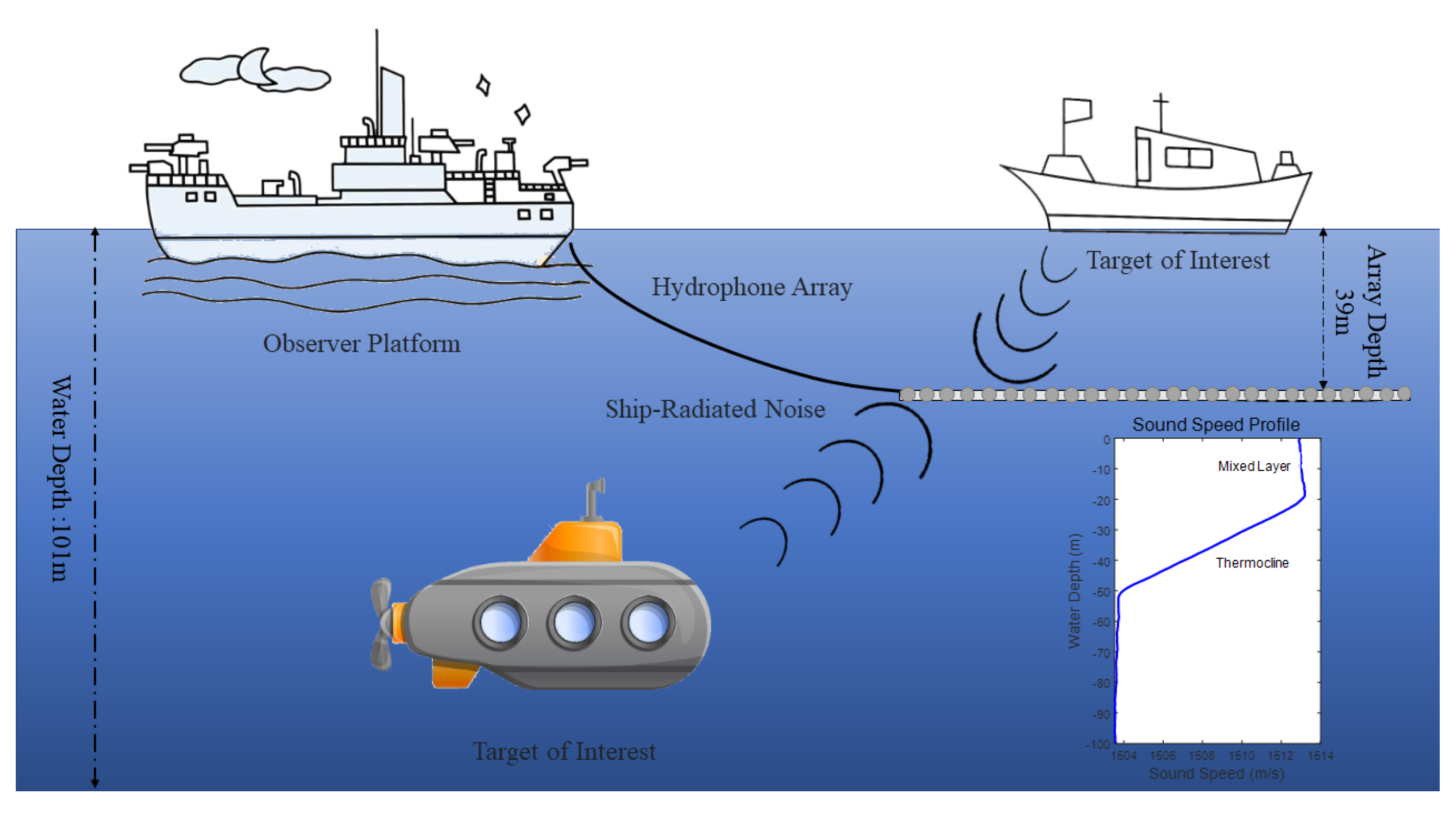
In multiple-target simulation, three targets initiated movement from 30 , 110 , and 140 , moving to 50 , 80 , and 150 , respectively, over a duration of 300 s with a time resolution of 1 s. Additionally, the amplitude ratios among these three targets were set at 1:0.33:0.5 over a duration of 300 s with a time resolution of 1 s per. The speed of sound of 1440 m/s is assumed, as well as a 256-unit uniform linear array spaced at d = 1.5 m. The frequency of the signal is 200 Hz, and the sampling frequency is 2000 Hz. The measuring signal angle ranges from 0 to 180 , with a precision of 0 . 5 . We employed CBF to process the received signals. Due to the translation invariance of the CBF directional function and considering the one-to-one mapping characteristics of the sine function, we observed that converting the original 0 to 180 angular range using the sine transform could result in multiple x-values corresponding to the same y-value. To ensure the uniqueness of angle conversion, we adjusted the angular range from −90 to 90 . This adjustment ensured the injectivity of the angular mapping, thus benefiting the accuracy and efficiency of subsequent data processing.
According to the steps in Section 3, we first perform open peak extraction on the single-frequency signals, selecting 200 Hz as the representative frequency for calculation for the CBF method. When f = 200 Hz, d = 1.5 m, and N = 256, the angle resolution of BTR is 0 . 5 . The main-to-sidelobe distance D s i d e is defined as the position of the maximum value of the first sidelobe. Since there is no analytical solution to Formula (6), through numerical simulation, we can obtain the main-to-sidelobe distance D s i d e 2 . 3 
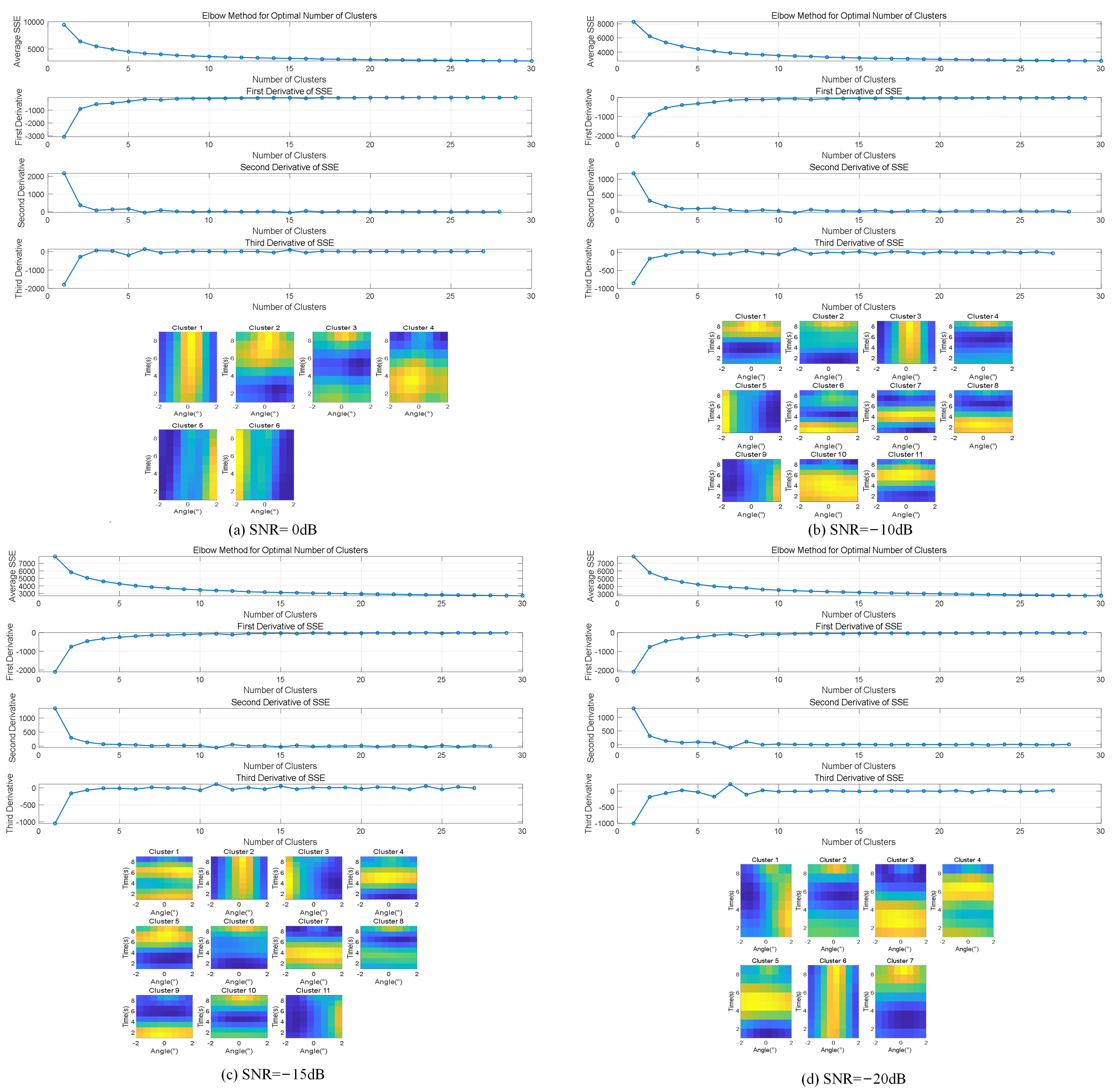
, so the width of the element should be nine pixels. We employed the improved k-means clustering algorithm on BTR for the first 300 frames. As shown in Figure 4, it automatically determined the optimal number of clusters to be 6, 11, 11, and 7 at SNR of 0 dB, −10 dB, −15 dB, and −20 dB; subsequently, we extracted the main lobe visual pattern, with size of 9 × 9 , which corresponds to the K A d a p t i v e . We used the 1D dCv method, the Theory 2D Conv method, the Gaussian Conv method, the Mean Conv method, and the Median Conv method for baselines and compared them with our proposed adaptive 2D method. We calculated a one-dimensional conventional kernel based on the corresponding array information, then obtained the K T h e o r y 2 D by accumulating K T h e o r y 1 D along the time dimension and expanding it to two dimensions. To match the K A d a p t i v e , whose size is 9 × 9 , the sizes of K T h e o r y 2 D , K G a u s s i a n , K M e a n , and K M e d i a n are also 9 × 9 . Then, we performed the convolution algorithm with the six conventional kernels and deconvolution beamforming in the last 100 frames of BTR.
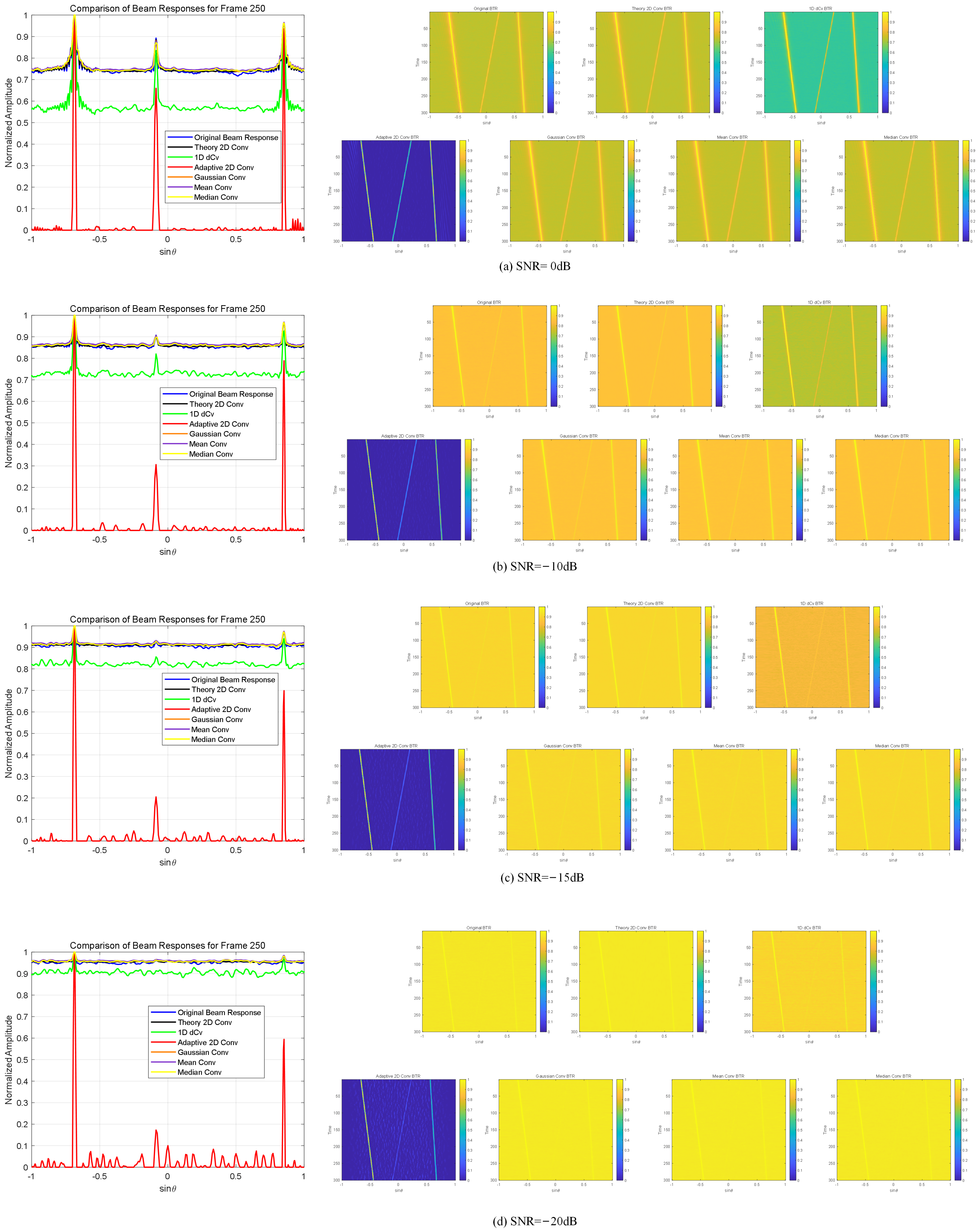
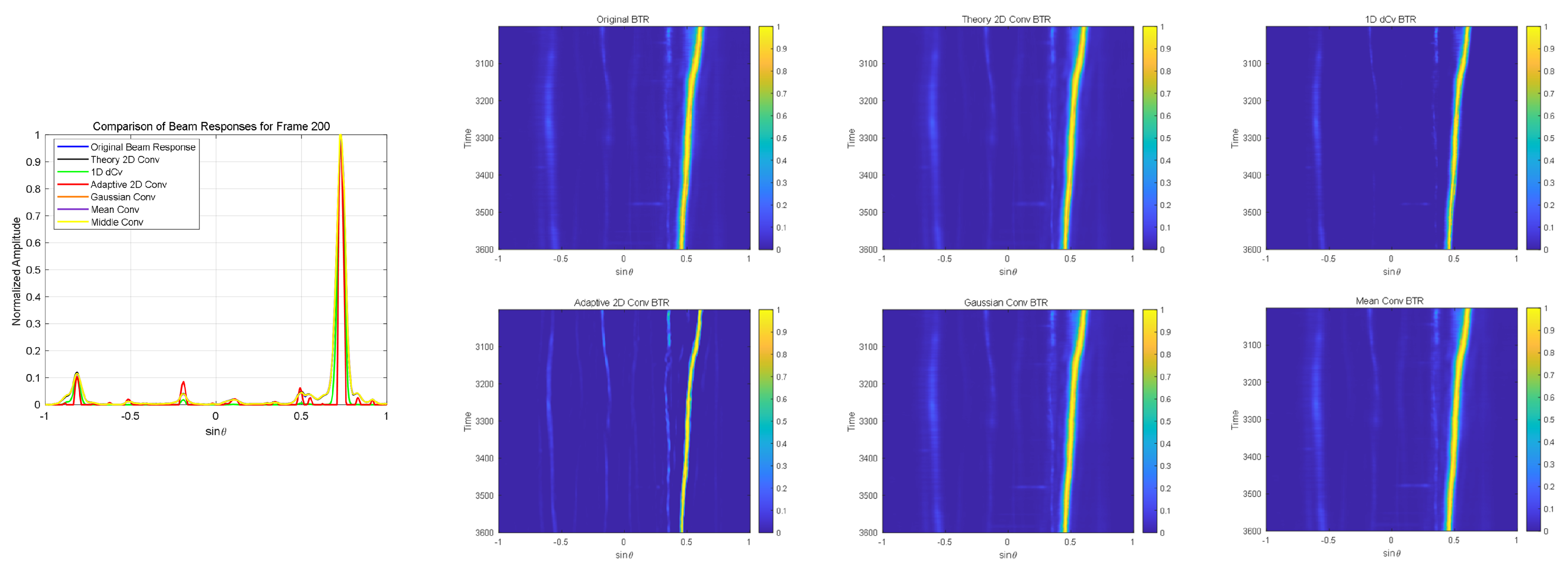
As shown in Table 1, by comparing the SNRs of the three targets for each method, the performance of the targets under different SNR conditions can be clearly observed. When SNR = 0 dB, the SNRs for Target 1, Target 2, and Target 3 using the CBF method are 2.5 dB, 1.73 dB, and 2.17 dB, respectively. The Theory 2D Conv method shows even lower SNRs, with values of 2.5 dB, 1.63 dB, and 2.16 dB, performing worse than the CBF method. The 1D dCv method shows a slight improvement, with SNRs of 4.75 dB, 3.93 dB, and 4.32 dB for the three targets. However, the Adaptive 2D Conv method provides a significant enhancement, yielding SNRs of 26 dB, 22.5 dB, and 25.4 dB, outperforming all other methods. The results for the Gaussian Conv, Mean Conv, and Median Conv methods are relatively similar. The Gaussian Conv method yields SNRs of 2.5 dB, 1.6 dB, and 2.17 dB, while the Mean Conv method produces SNRs of 1.41 dB, 1.58 dB, and 2.19 dB. The Median Conv method shows SNRs of 2.5 dB, 1.54 dB, and 2.16 dB, which are comparable to those of the Gaussian and Mean Conv methods.
When SNR = −10 dB, the CBF method shows a decrease in SNR, with values of 1.41 dB, 0.45 dB, and 1.1 dB for Target 1, Target 2, and Target 3, respectively. The Theory 2D Conv method performs similarly, with SNRs of 1.41 dB, 0.55 dB, and 1.1 dB. The 1D dCv method provides a slight improvement, yielding SNRs of 2.71 dB, 1.18 dB, and 2.16 dB. However, the Adaptive 2D Conv method shows a significant enhancement, maintaining high SNRs of 18.85 dB, 24.07 dB, and 20 dB, outperforming all other methods. In comparison, the Gaussian Conv and Mean Conv methods show similar performance, with SNRs of 1.41 dB, 0.5 dB, and 1.1 dB for Gaussian Conv and 1.41 dB, 0.52 dB, and 1.11 dB for Mean Conv. The Median Conv method produces SNRs of 1.41 dB, 0.45 dB, and 1.11 dB, which are comparable to the Gaussian and Mean Conv methods.
When SNR = −15 dB, the SNRs for all methods further decrease. The CBF method shows relatively low SNRs, with values of 0.63 dB, 0.12 dB, and 0.37 dB for the three targets, while the 1D dCv method provides a slight improvement, with SNRs of 0.92 dB, 0.17 dB, and 0.56 dB. The Theory 2D Conv method performs the worst, yielding even lower SNRs of 0.63 dB, 0.11 dB, and 0.37 dB, which are worse than both the CBF and 1D dCv methods. In contrast, the Adaptive 2D Conv method demonstrates strong performance, maintaining higher SNRs of 8.94 dB, 17.27 dB, and 7.27 dB, significantly outperforming all other methods. The results for the Gaussian Conv and Mean Conv methods are similar, with SNRs of 0.63 dB, 0.12 dB, and 0.38 dB for Gaussian Conv and 0.63 dB, 0.05 dB, and 0.37 dB for Mean Conv. The Median Conv method shows SNRs of 0.63 dB, 0.09 dB, and 0.35 dB, which are comparable to those of the Gaussian and Mean Conv methods.
As shown in the last line of subfigures of Figure 5, when SNR = −20 dB, due to the extremely low SNR, the weak energy targets are submerged by background noise, making it impossible to distinguish them in the original BTR obtained by CBF, as well as in the results obtained using other conventional or deconvolution algorithms. In contrast, our proposed Adaptive 2D Conv method is able to enhance the weak energy targets, allowing them to be differentiated from random noise. Notably, the Adaptive 2D Conv results show a more significant enhancement of the weak energy targets. Compared with the other methods, the Adaptive 2D Conv method has the narrowest main lobe width and nearly complete suppression of background noise. These results indicate that the Adaptive 2D Conv method significantly improves the target signal’s SNR under various conditions, especially in low SNR scenarios. This advantage makes the Adaptive 2D Conv method highly promising for practical applications, particularly for detecting weak targets by effectively suppressing background noise and maintaining high target distinguishability.

5. Sea-Trial Experiments

5.1. Dataset Description

In real sea trials, the underwater environment is highly complex due to surface conditions, vessel activity, and biological noise sources, making the background noise much stronger than in simulations. This creates two key challenges: it reduces the effectiveness of beamforming and limits the performance of later signal processing. To test the robustness of our method, we used real data from shallow-water trials, where depths ranged from 87.1 to 101 m. As shown in Figure 6, the system used a towed horizontal line array with 256 elements spaced 1.5 m apart. The passive detection system operated between 20 and 380 Hz. We compared our Adaptive 2D Conv method with CBF, Theory 2D Conv, 1D dCv, Gaussian Conv, Mean Conv, and Median Conv by analyzing the single-snapshot beam responses of BTR results. The dataset contains five targets over a 600-second period, with a time resolution of 1 s.

5.2. Performance Evaluations

We selected the center frequency of this broadband signal. When f = 200 Hz, d = 1.5 m, and N = 256, the angle resolution of BTR is 0 . 5 . The main-to-sidelobe distance D s i d e is defined as the position of the maximum value of the first sidelobe. Since there is no analytical solution to formula (6), through numerical simulation, we can obtain the main-to-sidelobe distance D s i d e 2 . 3 , so the width of the element should be 9 pixels. We employed the improved k-means clustering algorithm on BTR for the first 300 frames. As shown in Figure 7, it automatically determined the optimal number of clusters to be 3. Subsequently, we extracted the main lobe visual pattern, with size of 9 × 9 , which corresponds to the K A d a p t i v e . We use Theory 2D Conv, 1D dCv, Gaussian Conv, Mean Conv, and Median Conv for baselines and compare them with our proposed Adaptive 2D Conv. We calculated the K T h e o r y 1 D based on the corresponding array information and then obtain the K T h e o r y 2 D by accumulating K T h e o r y 1 D along the time dimension and expanding it to two dimensions. to match the K A d a p t i v e , whose size is 9 × 9 , so we obtained the size of K T h e o r y 2 D , K G a u s s i a n , K M e a n , and K M e d i a n are also 9 × 9 . Then, we performed dCv and Conv with the six conventional kernels in the last 300 frames of BTR.
As shown in Figure 8, it can be observed that the proposed Adaptive 2D Conv can significantly suppress background noise and narrow the main lobe width. To better compare the results, we extracted the single-frame data, as shown on the left of Figure 8. It can be seen that the proposed method has a significantly narrowed beam and lower background noise energy. At sin θ = 0.5 , two weak targets processed by conventional methods (including CBF, Theory 2D Conv, Gaussian Conv, Mean Conv, and Median Conv) are submerged by surrounding sidelobes or noise, making them prone to being misidentified as noise or sidelobes, leading to false negatives. Although the 1D dCv method shows some improvement, the target signal strength remains comparable to the background noise level, and the false negative problem persists. In contrast, applying the Adaptive 2D Conv method significantly enhances the weak target signals, allowing for clear separation of the two targets. At sin θ = 0.2 , the SNR is approximately 6 dB after processing with conventional methods (CBF, Theory 2D Conv, Gaussian Conv, Mean Conv, and Median Conv). With the 1D dCv method, the SNR increases slightly to 12 dB. However, after applying the Adaptive 2D Conv method, the SNR improves dramatically to 25 dB. At sin θ = 0.7 , where the target energy is strongest, the Adaptive 2D Conv method achieves the narrowest main lobe width, outperforming all other methods in terms of resolution.
To evaluate the real-time performance of the proposed method, we measured and compared the computation time of several BTR (Bearing-Time Record) denoising methods. The proposed Adaptive 2D Conv method consists of two stages: (1) extracting the point spread function (PSF) from historical BTR data and (2) performing convolution-based denoising using the extracted PSF. To ensure real-time applicability, the PSF is constructed using a sliding window of 300 snapshots. The kernel size is set to 9 × 9 , consistent with all baseline methods. The processing stride is set to 1 s, meaning one frame is processed per second. The evaluation was conducted using real sea-trial data with a total of 1200 snapshots. All methods were tested in MATLAB R2022a on a machine equipped with an Intel 12th Gen i7-12650H @ 2.30GHz. As shown in Table 2, each method’s total and per-frame processing times are reported.
The results show that although the proposed Adaptive 2D Conv method has slightly higher computational cost, it still achieves a per-frame processing time of approximately 0.31 s. This is sufficient for near real-time applications. Compared with faster but simpler filters such as Mean and Gaussian Conv, our method offers significantly better noise suppression and target enhancement, making it well-suited for practical underwater passive detection systems.

6. Conclusions

In the field of underwater detection, due to the complexity of ocean noise and the limitations of using array apertures, the obtained BTR often exhibits a low SNR and wide main lobes. In this paper, we propose the Adaptive 2D Conv for denoising and beam width narrowing in underwater acoustic BTRs. This method uses an improved k-means clustering algorithm to extract the visual pattern of the main lobe from BTR’s historical data as k A d a p t i v e , compared with the Theory 2D Conv, 1D dCv, Gaussian Conv, Mean Conv, and Median Conv in noise reduction and beam narrowing. More specifically, this method introduces an adaptive adaptive conventional kernel extracted from historical BTR into the underwater BTR convolution process, providing a novel method for resolution enhancement and noise suppression in the post-processing stage of underwater detection. Since the construction of an adaptive conventional kernel requires time information, it is primarily suitable for targets such as ships that continuously radiate noise. However, it is not applicable to targets like acoustic bombs that emit noise transiently. Under weak target detection with low SNR conditions, this method can effectively suppress sidelobes and random noise.

Author Contributions

Conceptualization, H.Y., C.L., H.W., J.W., F.Y., Z.Q. and C.W.; Methodology, H.Y. and C.L.; Software, H.Y. and C.L.; Validation, H.Y. and C.L.; Formal analysis, H.Y. and C.L.; Investigation, C.L., H.W., J.W., F.Y., Z.Q. and C.W.; Resources, C.L.; Data curation, C.L.; Writing—original draft preparation, H.Y. and C.L.; Writing—review and editing, C.L., H.W. and J.W.; Visualization, C.L.; Supervision, H.W. and J.W.; Project administration, C.L., H.W. and J.W.; Funding acquisition, C.L., H.W. and J.W. All authors have read and agreed to the published version of the manuscript.

Funding

This article is funded by the General Program of the National Natural Science Foundation of China (ID: 62171440), the project of the Chinese Academy of Sciences (ID: XDB0700403), and supported by the China Scholarship Council.

Data Availability Statement

The data are not publicly available due to privacy or ethical restrictions.

Conflicts of Interest

The authors declare that they have no known competing financial interests or personal relationships that could have appeared to influence.

References

  1. Capon, J. High-resolution frequency-wavenumber spectrum analysis. Proc. IEEE 1969, 57, 1408–1418. [Google Scholar] [CrossRef]
  2. Monzingo, R.A.; Miller, T.W. Introduction to Adaptive Arrays; Scitech Publishing: Raleigh, NC, USA, 2004. [Google Scholar]
  3. Krim, H.; Viberg, M. Two decades of array signal processing research: The par-ametric approach. IEEE Signal Process. Mag. 1996, 13, 67–94. [Google Scholar] [CrossRef]
  4. Van Trees, H.L. Optimum Array Processing: Part IV of Detection, Estimation, and Modulation Theory; John Wiley & Sons: Hoboken, NJ, USA, 2002. [Google Scholar]
  5. Cox, H. Resolving power and sensitivity to mismatch of optimum array proces-sors. J. Acoust. Soc. Am. 1973, 54, 771–785. [Google Scholar] [CrossRef]
  6. Rosenfeld, A.; Kak, A.C. Digital Picture Processing, 1st ed.; Academic Press: Cambridge, MA, USA, 1976. [Google Scholar]
  7. Li, Q.H.; Pan, X.; Yin, L. A new algorithm of background equalization. Chin. J. Acoust. 2000, 25, 5–9. [Google Scholar]
  8. Aharon, M.; Elad, M.; Bruckstein, A. K-SVD: An algorithm for designing over-complete dictionaries for sparse representation. IEEE Trans. Signal Process. 2006, 54, 4311–4322. [Google Scholar] [CrossRef]
  9. Buades, A.; Coll, B.; Morel, J.M. A non-local algorithm for image denoising. In Proceedings of the 2005 IEEE Computer Society Conference on Computer Vision and Pattern Recognition (CVPR’05), San Diego, CA, USA, 20–25 June 2005; pp. 2–9. [Google Scholar]
  10. Danielyan, A.; Katkovnik, V.; Egiazarian, K. BM3D frames and variational image deblurring. IEEE Trans. Image Process. 2011, 21, 1715–1728. [Google Scholar] [CrossRef] [PubMed]
  11. Dabov, A.; Foi, A.; Katkovnik, V.; Egiazarian, K. Image denoising by sparse 3-D transform-domain collaborative filtering. IEEE Trans. Image Process. 2007, 16, 2080–2095. [Google Scholar] [CrossRef] [PubMed]
  12. Yin, F.; Li, C.; Wang, H.; Nie, L.; Zhang, Y.; Liu, C.; Yang, F. Weak underwater acoustic target detection and enhancement with BM-SEED algorithm. J. Mar. Sci. Eng. 2023, 11, 357. [Google Scholar] [CrossRef]
  13. Yin, F.; Li, C.; Wang, H.; Yang, F. Automatic acoustic target detecting and tracking on the azimuth recording diagram with image processing methods. Sensors 2019, 19, 5391. [Google Scholar] [CrossRef] [PubMed]
  14. Yang, T.C. Deconvolved conventional beamforming for a horizontal line array. IEEE J. Ocean. Eng. 2018, 43, 160–172. [Google Scholar] [CrossRef]
  15. Yang, T.C. Deconvolved conventional beamforming applied to the SWellEx96 data. J. Acoust. Soc. Am. 2018, 144, 1768. [Google Scholar] [CrossRef]
  16. Yin, F.; Li, C.; Wang, H.; Zhou, S.; Nie, L.; Zhang, Y.; Yin, H. A robust denoised algorithm based on Hessian-sparse deconvolution for passive underwater acoustic detection. J. Mar. Sci. Eng. 2023, 11, 2028. [Google Scholar] [CrossRef]
  17. Richardson, W.H. Bayesian-based iterative method of image restoration. JoSA 1972, 62, 55–59. [Google Scholar] [CrossRef]
  18. Yin, H.; Li, C.; Wang, H.; Yin, F.; Yang, F. False alarm suppressing for passive underwater acoustic target de-tecting with computer visual techniques. Ocean. Eng. 2024, 305, 117969. [Google Scholar] [CrossRef]
Figure 1. Mismatch (red for strong target, green for weak target).
Jmse 13 01136 g001
Figure 2. Technical method.
Jmse 13 01136 g002
Figure 3. Element size and beamforming algorithms.
Jmse 13 01136 g003
Figure 4. Number of clusters with multiple targets.
Jmse 13 01136 g004
Figure 5. BTRs with multiple targets.
Jmse 13 01136 g005
Figure 6. Passive acoustic detection system layout.
Jmse 13 01136 g006
Figure 7. Number of culster with sea-trial experiments.
Jmse 13 01136 g007
Figure 8. BTRs with Sea-Trial Experiments.
Jmse 13 01136 g008
Table 1. Table of SNR values and corresponding targets.
SNR = 0 dBSNR = −10 dBSNR = −15 dB
T1T2T3T1T2T3T1T2T3
CBF2.51.732.171.410.451.100.630.120.37
Theory 2D Conv2.51.632.161.410.551.100.630.100.37
1D dCv4.753.934.322.711.182.160.920.170.56
Adaptive 2D Conv26.022.525.426.018.8524.0720.08.9417.27
Gaussian Conv2.51.602.171.410.501.100.630.120.38
Mean Conv2.51.582.191.410.521.110.630.0650.37
Median Conv2.51.542.161.410.451.110.630.090.35
Table 2. Computation time comparison for different methods.
MethodTotal Time (1200 Frames) (s)Average Time per Frame (s)
Adaptive 2D Conv372.510.310424
Theory 2D Conv252.240.210200
1D dCv202.760.168969
Mean Conv10.320.008596
Gaussian Conv11.930.009938
Median Conv28.990.024164
Disclaimer/Publisher’s Note: The statements, opinions and data contained in all publications are solely those of the individual author(s) and contributor(s) and not of MDPI and/or the editor(s). MDPI and/or the editor(s) disclaim responsibility for any injury to people or property resulting from any ideas, methods, instructions or products referred to in the content.

