Dynamic Analysis and Experimental Research on Anti-Swing Control of Distributed Mass Payload for Marine Cranes

Abstract

To address distributed mass payload (DMP) anti-swing control problems typified by offshore wind turbine blades, this paper adopts multi-body dynamics and rigid-flexible coupling modelling approaches. It derives the geometric constraints and static equilibrium equations for marine crane multipoint lifting of DMP, and establishes a dynamic coupling model considering ship roll and pitch environmental excitations. Then, under the maximum environmental excitation set in the experiment, the flexible cable parallel anti-swing system achieves swing suppression rates of 41.0% and 58.0% for the in-plane and out-of-plane angles of the DMP with regular geometric shape and mass distribution, respectively. For the DMP with irregular geometry and mass distribution, the suppression rates are 48.4% and 39.3% for the in-plane and out-of-plane angles, respectively. It is found that, after adjusting the lifting method and increasing the distance between the lifting points, the maximum in-plane angle of the payload decreases by 2.3%, while the out-of-plane angle maximum decreases by 52.0%. These results demonstrate the effectiveness of adjusting lifting methods in suppressing swing for irregular DMPs, thereby verifying the reliability and applicability of the flexible cable parallel anti-swing system and providing a reference for improving anti-swing performance and lifting efficiency in offshore DMP operations.

1. Introduction

Over the past century, with the continuous acceleration of human exploration of marine resources and the rapid development of the marine economy, the characteristics of offshore lifting operation scenarios, lifting objects, and lifting methods of marine cranes have diversified. In other words, marine cranes have not only been used to lift goods, but have also been involved in marine scientific research using AUVs (Autonomous Underwater Vehicles) and in offshore wind turbine lifting and docking operations for new energy applications. At the same time, the lifting objects have evolved from point-mass payloads to distributed mass payloads (DMPs), and the lifting methods have evolved from using a single lifting cable to multiple lifting cables. For example, the Haliade-X 12 MW wind turbine has a total height of 260 m, a blade length of 107 m, and a nacelle and rotor weight of 825 tonnes [1]. It was lifted and installed using an ultra-large offshore floating crane equipped with a parallel mechanism of multiple flexible cables. This DMP with an oversized geometric structure and mass distribution inevitably encounters wave excitation and wind disturbance during lifting operations, and then generates swing, which poses a major threat to the safety and efficiency of marine crane lifting operations.

At the same time, there is relatively little research on the dynamic analysis of the DMP for the flexible cable parallel anti-swing system of marine cranes. Most researchers focus their efforts on the anti-swing analysis of the point-mass payload, while the limited research on the anti-swing of DMP mainly concentrates on the anti-swing control methods for bridge cranes and tower cranes, such as command-smoothing control methods [2,3], adaptive control methods [4,5], trajectory planning methods [6], optimal command-smoothing methods [7], time-varying sliding mode control methods [8], equivalent rope length trajectory planning methods [9], and control methods based on deep reinforcement learning [10]. These anti-swing control methods still face many challenges and uncertainties in the DMP anti-swing control of marine cranes. In particular, internal friction in the marine crane system, unmodeled dynamics, parameter uncertainty, and other disturbances will make it difficult to ensure that the model-based design of the controller achieves the expected accuracy in practical applications. Meanwhile, from research progress and engineering applications of existing anti-swing technologies for marine crane payloads, the anti-swing studies on DMP mainly focus on optimising the mechanical structure design of cranes and developing new control methods. Therefore, this paper proposes a flexible cable parallel anti-swing system for dynamic analysis and anti-swing experimental research on DMP. In addition, the modelling method of simple pendulum for point-mass payload ignores the influence of the payload’s geometric structures and the positional differences between the centre and centre of gravity on swing control. This makes it difficult to accurately describe the payload’s swinging process and the dynamic response characteristics of the crane system. Therefore, the point-mass payload dynamic modelling method no longer meets the research and engineering application needs of anti-swing control for DMP.

In various marine engineering lifting operations, the flexible cable parallel anti-swing system has the characteristics of simple structure, light weight, flexible movement, and large working space. It plays an important role in large-scale, heavy-duty DMP lifting operations with a regular or irregular shape and mass distribution by virtue of the strong lifting capacity and stability advantage of multiple parallel cables. The world’s first prototype of a flexible cable parallel anti-swing system is the RoboCrane, which was developed by the National Institute of Standards and Technology (NIST) of the United States in 1989 [11]. The shape of this prototype is similar to that of an inverted Stewart mechanism, and the motion of the moving platform is controlled by six cables, which can be used for the handling of large goods, assembly, shipbuilding, and spraying. Gorman [12] introduced a specific cable-driven array robot with three drive cables; its geometric size is 1/16 that of the marine cranes used by the US Navy. The experimental studies show that the robot can track a given trajectory accurately with an error of a few centimetres. Hiller [13] designed and developed a cable-driven parallel mechanism named SEGESTA, which uses seven cables to control the six degrees of freedom of the moving platform. Bosscher [14] designed the Contour Crafting 4 (C4) system based on a multi-cable-driven parallel lifting mechanism with twelve cables, which can be used for the layered construction of large components. Afterwards, Lamaury [15] developed a six-degree-of-freedom cable-driven parallel redundant mechanism driven by eight cables, which can keep all driving cables in tension at all times, improving the tracking performance of the robot during cargo handling. There are also cable-driven parallel robots with under-constrained designs for cargo lifting. For example, Korayem [16] designed a six-degree-of-freedom parallel mechanism called ICASBOT with six cable drives, which is similar to the Robo Crane structure, and carried out prototype lifting experiments. Ren [1] studied the swing control of the large irregularly shaped payloads in offshore lifting operations by a multi-cable-driven parallel system, and proposed a lifting motion compensation scheme without model characteristics.

For offshore applications, the Large Vessel Interface Lift On/Lift Off (LVI LO/LO) is a prime example of the successful use of a flexible cable parallel anti-swing system in the lifting field. It is a parallel wave compensation system developed by the U.S. Navy Research Office in collaboration with Oceaneering and ATR, based on the 6-DOF parallel lifting robot RoboCrane [17]. This system represents a major breakthrough in advancing parallel wave compensation technology from theoretical research to practical application. Jung [18] and Kim [19,20] used machine vision and laser sensor technology to detect the spatial 6-DOF motion signals of the payload. They controlled the payload’s spatial position and attitude through multiple mechanisms, such as a double-deck overhead crane, rope tension sensors, and an intelligent platform. Finally, they developed a 1/20 scale prototype to carry out payload motion compensation experiments. However, compared with the LVI LO/LO, the system they designed has a complex mechanical structure and poor practicability. Furthermore, Hu [21] proposed an eight-cable-driven parallel wave compensation device, which can effectively suppress the swing of the payload. This device changes the cable arrangement of the crane and also affects the lifting operation space. In addition, the telescopic sleeve rigid-flexible coupling anti-swing technology [22] and flexible cable-driven parallel mechanism multipoint collaborative lifting technology [23,24] have emerged in recent years. These technologies have improved the anti-swing effect by optimising the mechanical structure design of the marine crane anti-swing system and innovating control methods, and have been applied in engineering practice. Meanwhile, the adaptive controller [25], a nonlinear anti-swing controller based on asymmetric barrier Lyapunov functions [26], and the neuroendocrine PID [27] controller offer advantages in the control of complex, nonlinear time-varying underactuated systems in marine cranes systems. However, these algorithms are significantly limited by the fact that the design and implementation of the controller is complex and requires a large amount of training data and computational resources. To address the issue of the swing control of marine cranes when they are lifting heavy payloads, Zhu [28] designed a multi-cable-driven series-parallel hybrid pull-block anti-swing device.

In addition, when lifting large equipment, such as wind turbine blades and tower barrels, there is also a man-machine collaborative lifting method composed of “crane—DMP—tagline system—auxiliary personnel”. The tagline system plays a very important role in this lifting method as it acts as a balancing, fixing, and anti-swing cable. To ensure lifting safety, taglines are usually tied to the bottom of the payload (DMP) or a specialised spreader. Operators on the ground or platform assist with pulling the tagline or use a winch-driven wire guide system to control tagline tension, thus completing payload swing suppression through auxiliary methods. However, the payload is highly susceptible to wind-induced swing during the DMP lifting process, and the swing suppression method using the tagline system and human assistance has posed certain risks due to insufficient control capability. Eltronic and High Wind have developed two active control systems with taglines, namely the Tagline Master and the Boom Lock—Tagline Systems [29,30]. The former mainly controls the tension of the tagline through multiple winches to achieve automatic stabilisation control, while the latter uses a cantilever that can move with the crane boom to lock the hook to the crane boom, controlling the stability of the hook in high wind speeds at high altitudes, and working together with other auxiliary cables located on the spreader to significantly suppress the swing of the crane payload. They are mainly used for swing control of the tower, engine room, and blade parts during offshore wind power installation.

This paper focuses on the kinematic and static modelling of the lifting operation of the DMP within the flexible cable parallel anti-swing system for marine cranes. Additionally, a dynamic coupling model of the ship—a flexible cable parallel anti-swing system of the marine crane—DMP under roll and pitch environmental disturbances is established. At the same time, the flexible cable parallel anti-swing system of the marine crane is used to conduct experimental studies on the anti-swing dynamics of DMP with regular/irregular geometrical shapes and mass distributions under different lifting methods.

The paper is organised as follows: the kinematic and static modelling and analysis of the marine crane flexible cable parallel anti-swing system are carried out in Section 2. The coupled dynamic modelling of the marine crane flexible cable parallel anti-swing system DMP under environmental disturbances is presented in Section 3. The DMP anti-swing experiments under different lifting methods are carried out in Section 4. Finally the paper is summarised in Section 5.

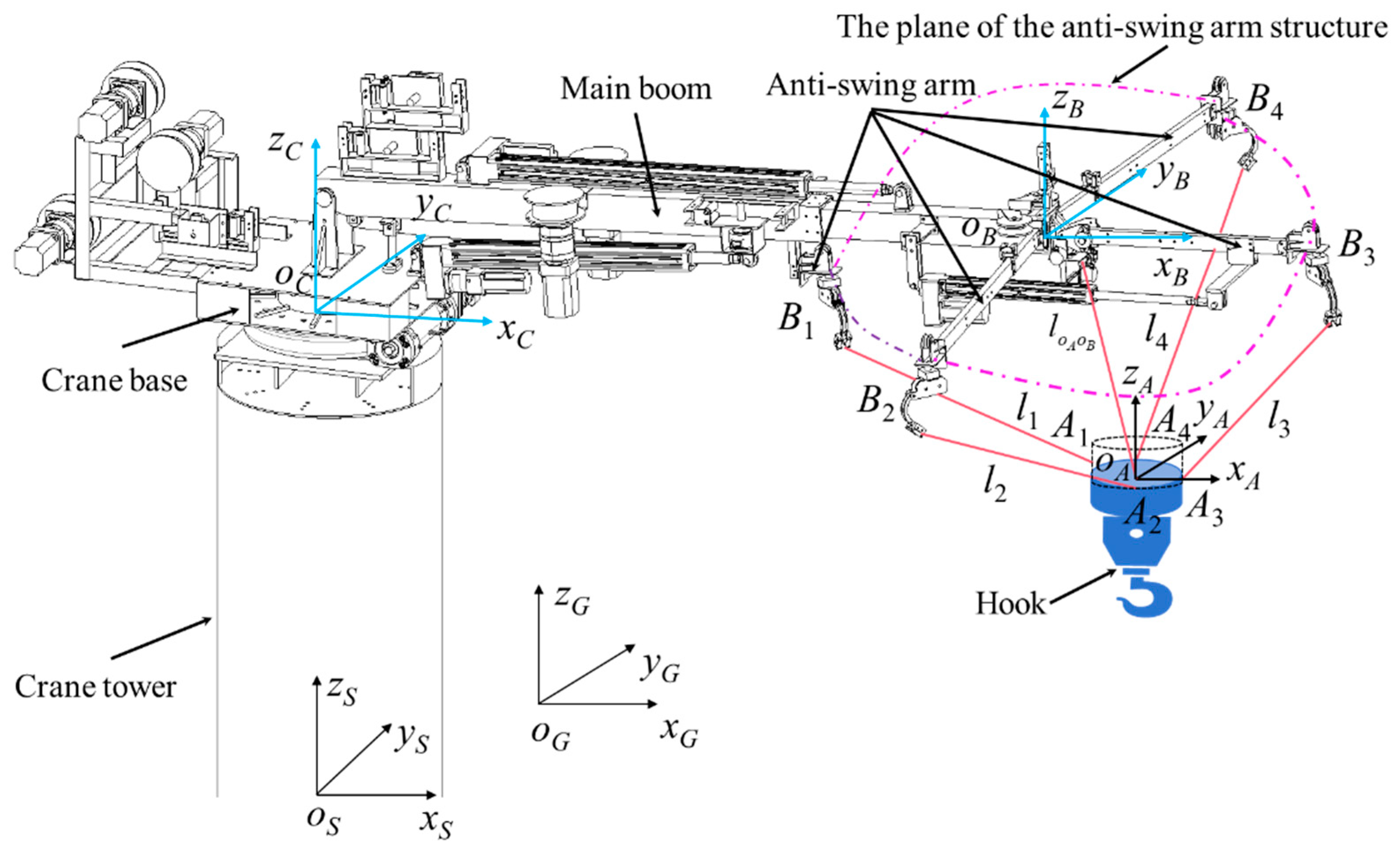
2. Kinematic and Static Modelling and Analysis

The flexible cable parallel anti-swing system described in this paper is a mechanical device, which generally consists of multiple flexible cables (≥3), driving device, sensors, and a control unit [31]. One end of the flexible cables is directly connected to the payload, while the other end is connected to the marine crane driving device through a steering pulley system. Multiple flexible cables form a parallel structure in three-dimensional space and work together to control the movement of the payload.

DMP is a type of payload whose mass distribution changes with the change in geometry, which is characterised by uneven mass and irregular geometry. Therefore, for marine cranes performing DMP lifting, the payload cannot be directly simplified into a particle model during dynamic modelling. Instead, a dynamic model that comprehensively reflects the multi-body rigid-flexible coupling effect between the DMP and the flexible cable parallel anti-swing mechanism of the marine crane should be established based on the structural characteristics of the DMP itself.

As shown in Figure 1, the marine crane flexible cable parallel anti-swing system mainly consists of the crane base, tower, main crane boom, anti-swing arm, hook and payload. The inertial coordinate system is o_G–x_Gy_Gz_G, the crane base coordinate system is o_S–x_Sy_Sz_S, and the crane boom slewing coordinate system is o_C–x_Cy_Cz_C. The plane coordinate system where the anti-swing arm structure is located is o_B–x_By_Bz_B, and the dynamic plane coordinate system in which the payload system is located is o_A–x_Ay_Az_A. B_i (i = 1, 2, 3, 4) is the fixed anchor point. In robotics, the fixed anchor point refers to the cable guide pulley and fixed seat with rotational degrees of freedom; the rotation axis of the cable guide pulley’s circular surface coincides with the direction of the incoming rope; and its tangent point position remains unchanged when the rope is being retracted or released [32,33]. This refers to the connection point between the i-th anti-swing cable and the anti-swing arm structure. A_i (i = 1, 2, 3, 4) is the connection point between the i-th anti-swing cable and the plane where the payload system is located, also known as the dynamic platform connection point. $l_{o_A{o}_B}$ is the main sling of the marine crane. The attitude description of the moving platform is expressed in terms of the Euler angles of rotation around the x-axis, y-axis, and z-axis of the inertial coordinate system in turn, and conforms to the right-hand rule.

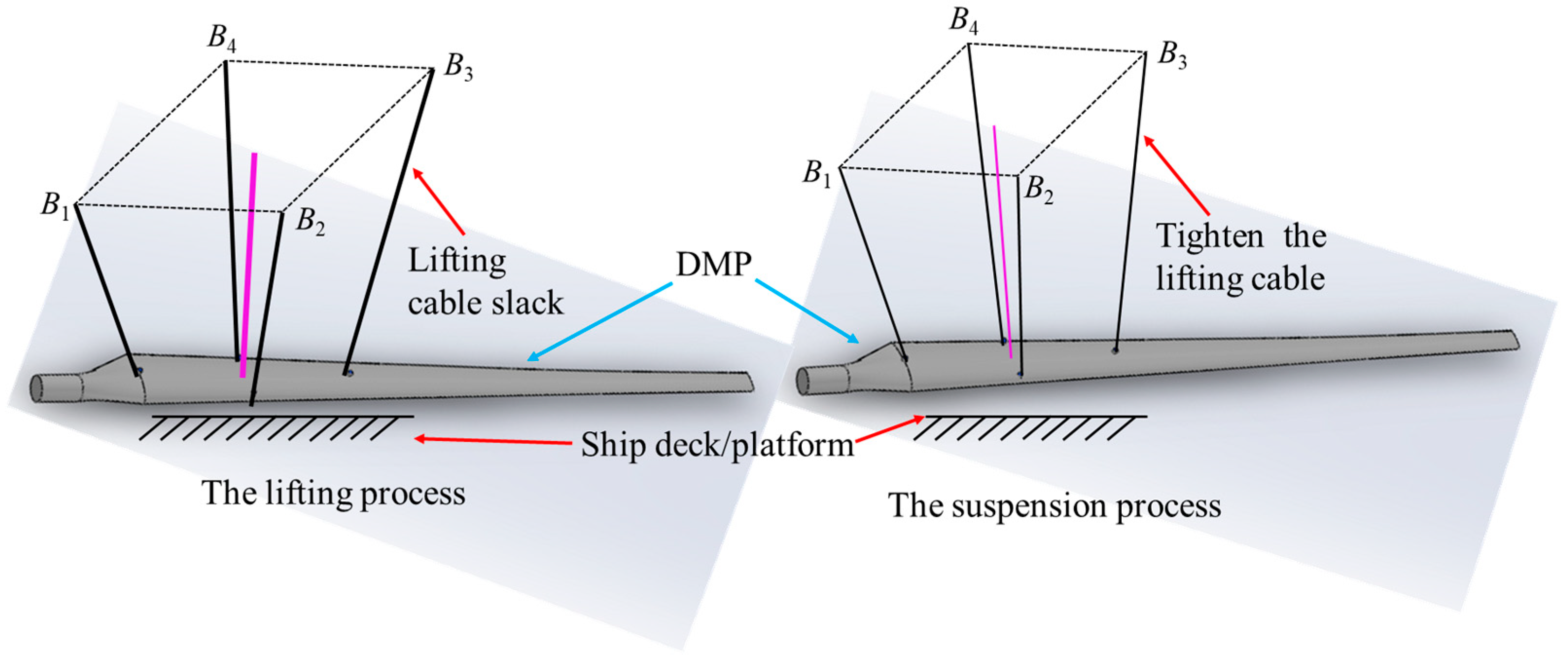
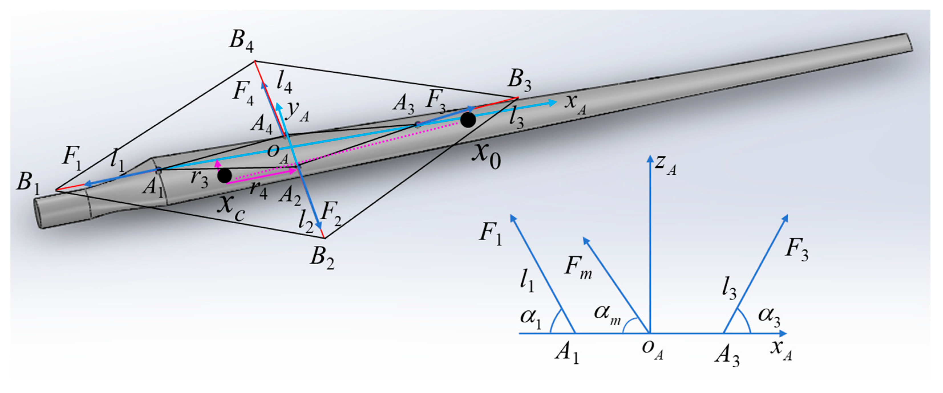
2.1. Kinematics of a Flexible Cable Parallel Anti-Swing System

In robotics, the process of calculating the joint angle of the manipulator arm with the known position of the end moving platform is defined as the inverse solution, while in the flexible cable parallel anti-swing system of the marine crane, it refers to the known swing angle and attitude position of the hook and the payload in the space, to calculate the cable length of the anti-swing cable. The real-time attitude of the moving platform, where the marine crane hook and payload are located in the inertial coordinate system, is defined as P = [x y z α β γ]^T. Accordingly, the homogeneous transformation matrix T from the moving coordinate system to the inertial coordinate system can be derived as follows:

The detailed expressions for the matrices in Equation (1) are,

$$\mathit{T}=\mathit{Tans}(x,y,z)\mathit{R}=\mathit{Tans}(x,y,z)R(z,\gamma )R(y,\beta )R(x,\alpha )=\left[\begin{array}{cccc}1& 0& 0& x\\ 0& 1& 0& y\\ 0& 0& 1& z\\ 0& 0& 0& 1\end{array}\right]\left[\begin{array}{cc}R& \mathbf{0}\\ \mathbf{0}& \mathbf{1}\end{array}\right]$$

(1)

$$R(z,\gamma )=\left[\begin{array}{ccc}\cos \gamma & -\sin \gamma & 0\\ \sin \gamma & \cos \gamma & 0\\ 0& 0& 1\end{array}\right], R(y,\beta )=\left[\begin{array}{ccc}\cos \beta & 0& \sin \beta \\ 0& 1& 0\\ -\sin \beta & 0& \cos \beta \end{array}\right], R(x,\alpha )=\left[\begin{array}{ccc}1& 0& 0\\ 0& \cos \alpha & -\sin \alpha \\ 0& \sin \alpha & \cos \alpha \end{array}\right].$$

where, Trans(x, y, z) is a 4 × 1 offset vector, R is a rotation matrix, α, β and γ are Euler angles, and 0 denotes a zero vector, ensuring consistency with the 4 × 4 homogeneous transformation matrix.

The vectors pointing from the origin o_B of the plane coordinate system o_B–x_By_Bz_B where the crane anti-swing arm structure is located and the origin o_A of the plane dynamic coordinate system o_A–x_Ay_Az_A of the payload system to the respective anti-swing cable connection points are defined as b_i and a_i, respectively. Thus, $b_i=\overrightarrow{o_B{B}_i}$ and $a_i=\overrightarrow{o_A{A}_i}$ can be obtained, and at the same time, the length of each anti-swing cable can be expressed as,

$$l_i=\overrightarrow{A_i{B}_i}=\overrightarrow{o_B{B}_i}-\overrightarrow{o_A{A}_i}=b_i-a_i$$

(2)

The position of the moving coordinate system o_A relative to the coordinate system o_B is defined as ${\mathbf{x}}_{o_A{o}_B}={[\begin{array}{ccc}x& y& z\end{array}]}^{\mathrm{T}}$. Then, Equation (2) becomes

$$l_i=b_i-{\mathbf{x}}_{o_A{o}_B}-a_i$$

(3)

Furthermore, the calculation formula of the cable length expression of each anti-swing cable shown in Equation (3) can be obtained in the coordinate system o_B.

$$l_i^{o_B}=b_i^{o_B}-R_{o_D}^{o_B}{\mathbf{x}}_{o_A{o}_D}^{o_D}-{\mathbf{x}}_{{o_D}_{o_B}}^{o_B}-R_{o_C}^{o_B}{R}_{o_S}^{o_C}{R}_{o_A}^{o_S}{a}_i^{o_A}$$

(4)

Since the magnitudes of a_i and b_i are fixed in the flexible cable parallel anti-swing system of the marine crane and can be measured directly by using appropriate tools, according to ${\mathbf{x}}_{{o_A}_{o_B}}^{o_B}=R_{o_D}^{o_B}{\mathbf{x}}_{{o_A}_{o_D}}^{o_D}+{\mathbf{x}}_{{o_D}_{o_B}}^{o_B}$ and $R_{o_A}^{o_B}=R_{o_C}^{o_B}{R}_{o_S}^{o_C}{R}_{o_A}^{o_S}$, the expression for the length of each anti-swing cable l_i is obtained from Equation (4) as follows:

$$l_i=\left|l_i^{o_B}\right|=\sqrt{{(l_i^{o_B})}^{\mathrm{T}}{l}_i^{o_B}}=\sqrt{{(b_i^{o_B}-{\mathbf{x}}_{{o_A}_{o_B}}^{o_B}-R_{o_A}^{o_B}{a}_i^{o_A})}^{\mathrm{T}}(b_i^{o_B}-{\mathbf{x}}_{{o_A}_{o_B}}^{o_B}-R_{o_A}^{o_B}{a}_i^{o_A})}$$

(5)

In this way, the inverse kinematic model of the payload anti-swing process of the marine crane flexible cable parallel anti-swing system is obtained.

$$f_i({}^{o_A}A_i,{}^{o_B}B_i,\mathit{P})=0$$

(6)

where, ${}^{o_A}A_i$ denotes the coordinates of point A_i in the o_A coordinate system, and ${}^{o_B}B_i$ denotes the coordinates of point B_i in the o_B coordinate system.

Notably, in solving the inverse kinematic model of the payload anti-swing in the marine crane flexible cable parallel anti-swing system, if the expected position of the payload relative to the ship deck is set and the attitude relative to the ship deck is obtained, the length of anti-swing cable that needs to be retracted and released by the winch during the payload anti-swing control process can be calculated according to Equation (5). Thus, adjusting the winch actions directly to match these calculated lengths enables effective suppression of payload swing.

In robotics, the process of calculating the attitude of the end moving platform based on the known joint angle of the manipulator arm is defined as the positive solution. Similarly, in the forward kinematics of the payload anti-swing in marine crane with a flexible cable parallel anti-swing system, it refers to the known length of the anti-swing cable to calculate the swing angle and the attitude of the hook and payload in the three-dimensional space. According to the relationship between the number of cables m and the number of degrees of freedom n of the end moving platform, the flexible cable-driven parallel robot can be divided into redundant constrained type (m ≥ n), fully constrained type (m = n), and unconstrained type (m ≤ n).

The kinematic model obtained by Equation (6) is represented by vector $f^0$,

$$f^0={[\begin{array}{lllll}{f}_1^0\hfill & f_2^0\hfill & f_3^0\hfill & f_4^0\hfill & f_{o_A{o}_B}^0\hfill \end{array}]}^T=\left[\begin{array}{c}{f}_1({}^{o_A}A_1,{}^{o_B}B_1,\mathit{P})\\ f_2({}^{o_A}A_2,{}^{o_B}B_2,\mathit{P})\\ f_3({}^{o_A}A_3,{}^{o_B}B_3,\mathit{P})\\ \begin{array}{l}{f}_4({}^{o_A}A_4,{}^{o_B}B_4,\mathit{P})\\ f_5({}^{o_A}x_{o_A},{}^{o_B}x_{o_A},\mathit{P})\end{array}\end{array}\right]=0$$

(7)

Considering that there are four anti-swing cables and one main sling in the cable parallel anti-swing system of the marine crane in Figure 1, and that the end moving platform has six degrees of freedom, it is an under-constrained model. Combining Equations (6) and (7), it can be seen that the kinematic model of the flexible cable parallel anti-swing system is five nonlinear equations with six unknowns, with multiple possible solutions. From the kinematic analysis, it can be seen that when the length of the four anti-swing cables is fixed, the attitude of the hook and payload still cannot be determined, mainly due to the external force and external torque. Therefore, in order to accurately obtain the attitude of the hook and payload, it is necessary to solve the kinematic and static equilibrium equations of the payload system. Therefore, the under-constrained model schematic of the flexible cable parallel anti-swing system of a marine crane is established, as shown in Figure 2.

At a certain point in time, the external force generated by the excitation of the external environment and the gravity of the payload system acts on point G, represented by Q. L_e is the normalised Plücker vector of its action line, and ρ_i denotes the length of the i-th cable (i = 1, 2, 3, 4, 5). At this time, the global coordinate system $o^{\prime }-x^{\prime }{y}^{\prime }{z}^{\prime }$ is a Cartesian coordinate system established at the connection point B_i of the fixed anchor point on the anti-swing arm behind the main boom of the marine crane. Point B₄ is in the $x^{\prime }-z^{\prime }$ plane, and the direction of the $z^{\prime }$ axis is in the same direction as L_e. The dynamic coordinate system $o^{″}-x^{″}{y}^{″}{z}^{″}$ is a Cartesian coordinate system established on the dynamic platform where the marine crane payload system is located. Point A₄ is in the $x^{″}-z^{″}$ plane, so the position vectors of points A₁, A₂, A₃, A₄, B₁, B₂, B₃, B₄, and G in the $o^{\prime }-x^{\prime }{y}^{\prime }{z}^{\prime }$ coordinate system can be obtained. The result is shown below:

$$\begin{array}{c}{\mathit{a}}_{o_A}^{\prime }={[\begin{array}{ccc}{x}_{o_A}^{\prime }& y_{o_A}^{\prime }& z_{o_A}^{\prime }\end{array}]}^T, {\mathit{a}}_1^{\prime }={[\begin{array}{ccc}{x}_1^{\prime }& y_1^{\prime }& z_1^{\prime }\end{array}]}^T, {\mathit{a}}_2^{\prime }={[\begin{array}{ccc}{x}_2^{\prime }& y_2^{\prime }& z_2^{\prime }\end{array}]}^T, {\mathit{a}}_3^{\prime }={[\begin{array}{ccc}{x}_3^{\prime }& y_3^{\prime }& z_3^{\prime }\end{array}]}^T,\hfill \\ {\mathit{a}}_3^{\prime }={[\begin{array}{ccc}{x}_4^{\prime }& y_4^{\prime }& z_4^{\prime }\end{array}]}^T, \mathit{g} \prime ={[\begin{array}{ccc}{g}_x^{\prime }& g_y^{\prime }& g_z^{\prime }\end{array}]}^T, {\mathit{b}}_{o_B}^{\prime }={[\begin{array}{ccc}{x}_{o_B}^{\prime }& y_{o_B}^{\prime }& z_{o_B}^{\prime }\end{array}]}^T, {\mathit{b}}_1^{\prime }={[\begin{array}{ccc}0& 0& 0\end{array}]}^T,\hfill \\ {\mathit{b}}_2^{\prime }={[\begin{array}{ccc}{b}_{2x}^{\prime }& b_{2y}^{\prime }& b_{2z}^{\prime }\end{array}]}^T, {\mathit{b}}_3^{\prime }={[\begin{array}{ccc}{b}_{3x}^{\prime }& b_{3y}^{\prime }& b_{3z}^{\prime }\end{array}]}^T, {\mathit{b}}_4^{\prime }={[\begin{array}{ccc}{b}_{4x}^{\prime }& 0& b_{4z}^{\prime }\end{array}]}^T.\hfill \end{array}$$

Similarly, the position vectors of points A₁, A₂, A₃, A₄, and G in the $o^{″}-x^{″}{y}^{″}{z}^{″}$ coordinate system can be obtained. The results are as follows:

$$\begin{array}{c}{\mathit{a}}_{o_A}^{″}={[\begin{array}{ccc}{x}_{o_A}^{″}& y_{o_A}^{″}& z_{o_A}^{″}\end{array}]}^T, {\mathit{a}}_1^{″}={[\begin{array}{ccc}0& 0& 0\end{array}]}^T, {\mathit{a}}_2^{″}={[\begin{array}{ccc}{x}_2^{″}& y_2^{″}& z_2^{″}\end{array}]}^T, {\mathit{a}}_3^{″}={[\begin{array}{ccc}{x}_3^{″}& y_3^{″}& z_3^{″}\end{array}]}^T,\hfill \\ {\mathit{a}}_4^{″}={[\begin{array}{ccc}{x}_4^{″}& 0& y_4^{″}\end{array}]}^T, {\mathit{g}}^{″}={[\begin{array}{ccc}{g}_x^{″}& g_y^{″}& g_z^{″}\end{array}]}^T.\hfill \end{array}$$

To maintain a good anti-swing effect, the four anti-swing cables and the main sling of the marine crane are kept under tension during the lifting operation. At this point, the geometric constraint relationship of the moving platform where the payload system is located is as follows:

$${‖{\mathit{a}}_i^{\prime }-{\mathit{b}}_i^{\prime }‖}^2={\mathit{\rho }}_i^2$$

(8)

Based on the previous definitions of the coordinates of each point, Equation (8) is further optimised to obtain the following expression:

$$\left\{\begin{array}{l}{(x_2^{\prime }-x_1^{\prime })}^2+{(y_2^{\prime }-y_1^{\prime })}^2+{(z_2^{\prime }-z_1^{\prime })}^2={‖{\mathit{a}}_2^{″}‖}^2\hfill \\ {(x_3^{\prime }-x_1^{\prime })}^2+{(y_3^{\prime }-y_1^{\prime })}^2+{(z_3^{\prime }-z_1^{\prime })}^2={‖{\mathit{a}}_3^{″}‖}^2\hfill \\ {(x_4^{\prime }-x_1^{\prime })}^2+{(y_4^{\prime }-y_1^{\prime })}^2+{(z_4^{\prime }-z_1^{\prime })}^2={‖{\mathit{a}}_4^{″}‖}^2\hfill \\ {(x_3^{\prime }-x_2^{\prime })}^2+{(y_3^{\prime }-y_2^{\prime })}^2+{(z_3^{\prime }-z_2^{\prime })}^2={‖{\mathit{a}}_4^{″}-{\mathit{a}}_2^{″}‖}^2\hfill \\ {(x_4^{\prime }-x_2^{\prime })}^2+{(y_4^{\prime }-y_2^{\prime })}^2+{(z_4^{\prime }-z_2^{\prime })}^2={‖{\mathit{a}}_3^{″}-{\mathit{a}}_2^{″}‖}^2\hfill \\ {(x_4^{\prime }-x_3^{\prime })}^2+{(y_4^{\prime }-y_3^{\prime })}^2+{(z_4^{\prime }-z_3^{\prime })}^2={‖{\mathit{a}}_3^{″}-{\mathit{a}}_4^{″}‖}^2\hfill \\ {(x_1^{\prime }+x_{oA}^{\prime })}^2+{(y_1^{\prime }+y_{oA}^{\prime })}^2+{(z_1^{\prime }+z_{o_A}^{\prime })}^2={‖{\mathit{a}}_{oA}^{″}‖}^2\end{array}\right.$$

(9)

Since the position and attitude of the moving platform where the hook and the payload are located are determined by the static equilibrium equation, the normalised Plücker vector of the i-th cable can be defined as ${\mathit{L}}_i/{\mathit{\rho }}_i$, and ${\mathit{L}}_i={\left[\begin{array}{c}{\mathit{a}}_i^{\prime }-{\mathit{b}}_i^{\prime }\\ {\mathit{\rho }}_i\times ({\mathit{a}}_i^{\prime }-{\mathit{b}}_i^{\prime })\end{array}\right]}^{\mathrm{T}}$, ${\mathit{\rho }}_i$ is any vector from any reference point P to the lifting cable. At the same time, the wrench of the i-th hoisting cable acting on the moving platform of the marine crane is obtained as ${\mathit{L}}_i{\tau }_i/{\rho }_i$ (${\tau }_i>0$), and ${\tau }_i$ is the driving force of the hoisting cable. Thus, the static equilibrium equation of the moving platform in the unconstrained model of the marine crane flexible cable parallel anti-swing system is obtained.

$$\left[\begin{array}{llllll}{\mathit{L}}_1\hfill & {\mathit{L}}_2\hfill & {\mathit{L}}_3\hfill & {\mathit{L}}_4\hfill & {\mathit{L}}_{o_B{o}_A}\hfill & {\mathit{L}}_e\hfill \end{array}\right]{\left[\begin{array}{llllll}{\tau }_1/{\rho }_1\hfill & {\tau }_2/{\rho }_2\hfill & {\tau }_3/{\rho }_3\hfill & {\tau }_4/{\rho }_4\hfill & {\tau }_5/{\rho }_{o_B{o}_A}\hfill & Q\hfill \end{array}\right]}^{\mathrm{T}}=0$$

(10)

When $\mathit{M}(P)=\left[\begin{array}{llllll}{\mathit{L}}_1\hfill & {\mathit{L}}_2\hfill & {\mathit{L}}_3\hfill & {\mathit{L}}_4\hfill & {\mathit{L}}_{o_B{o}_A}\hfill & {\mathit{L}}_e\hfill \end{array}\right]$, then there is,

$$\mathit{M}(P)=\left[\begin{array}{cccccc}{x}_1^{\prime }& x_2^{\prime }-b_{2x}^{\prime }& x_3^{\prime }-b_{3x}^{\prime }& x_4^{\prime }-b_{2x}^{\prime }& x_{o_A}^{\prime }-x_{o_B}^{\prime }& 0\\ y^{\prime }& y_2^{\prime }-b_{2y}^{\prime }& y_3^{\prime }-b_{3y}^{\prime }& y_4^{\prime }& y_{o_A}^{\prime }-y_{o_B}^{\prime }& 0\\ z_1^{\prime }& z_2^{\prime }-b_{2z}^{\prime }& z_3^{\prime }-b_{3z}^{\prime }& z_4^{\prime }-b_{4x}^{\prime }& z_{o_A}^{\prime }-z_{o_B}^{\prime }& -1\\ 0& y_2^{\prime }{b}_{2z}^{\prime }-z_2^{\prime }{b}_{2y}^{\prime }& y_3^{\prime }{b}_{3z}^{\prime }-z_3^{\prime }{b}_{3y}^{\prime }& y_4^{\prime }{b}_{4z}^{\prime }& y_{o_A}^{\prime }{z}_{o_B}^{\prime }-y_{o_B}^{\prime }{z^{\prime }}_{o_A}& -g_y^{\prime }\\ 0& z_2^{\prime }{b}_{2x}^{\prime }-x_2^{\prime }{b}_{2z}^{\prime }& z_3^{\prime }{b}_{3x}^{\prime }-x_3^{\prime }{b}_{3z}^{\prime }& z_4^{\prime }{b}_{4x}^{\prime }-x_4^{\prime }{b}_{4z}^{\prime }& x_{o_B}^{\prime }{z}_{o_A}^{\prime }-x_{o_A}^{\prime }{z}_{o_B}^{\prime }& g^{\prime }\\ 0& x_2^{\prime }{b}_{2y}^{\prime }-y_2^{\prime }{b}_{2x}^{\prime }& x_3^{\prime }{b}_{3y}^{\prime }-y_3^{\prime }{b}_{3x}^{\prime }& -y_4^{\prime }{b}_{4x}^{\prime }& x_{o_A}^{\prime }{y}_{o_B}^{\prime }-x_{o_B}^{\prime }{y}_{o_A}^{\prime }& 0\end{array}\right]$$

(11)

Substituting Equation (11) into Equation (10), we have

$$\left\{\begin{array}{l}{\displaystyle \frac{{\tau }_1{x}_1^{\prime }}{{\rho }_1}}+{\displaystyle \frac{{\tau }_2(x_2^{\prime }-b_{2x}^{\prime })}{{\rho }_2}}+{\displaystyle \frac{{\tau }_3(x_3^{\prime }-b_{3x}^{\prime })}{{\rho }_3}}+{\displaystyle \frac{{\tau }_4(x_4^{\prime }-b_{4x}^{\prime })}{{\rho }_4}}+{\displaystyle \frac{{\tau }_5(x_{o_A}^{\prime }-x_{o_B}^{\prime })}{{\rho }_{o_B{o}_A}}}=0\hfill \\ {\displaystyle \frac{{\tau }_1{y}_1^{\prime }}{{\rho }_1}}+{\displaystyle \frac{{\tau }_2(y_2^{\prime }-b_{2y}^{\prime })}{{\rho }_2}}+{\displaystyle \frac{{\tau }_3(y_3^{\prime }-b_{3y}^{\prime })}{{\rho }_3}}+{\displaystyle \frac{{\tau }_4{y}_4^{\prime }}{{\rho }_4}}+{\displaystyle \frac{{\tau }_5(y_{o_A}^{\prime }-y_{o_B}^{\prime })}{{\rho }_{o_B{o}_A}}}=0\hfill \\ {\displaystyle \frac{{\tau }_1{z^{\prime }}_1}{{\rho }_1}}+{\displaystyle \frac{{\tau }_2(z_2^{\prime }-b_{2z}^{\prime })}{{\rho }_2}}+{\displaystyle \frac{{\tau }_3(z_3^{\prime }-b_{3z}^{\prime })}{{\rho }_3}}+{\displaystyle \frac{{\tau }_4(z_4^{\prime }-b_{4z}^{\prime })}{{\rho }_4}}+{\displaystyle \frac{{\tau }_5(z_{o_A}^{\prime }-z_{o_B}^{\prime })}{{\rho }_{o_B{o}_A}}}-Q=0\hfill \\ {\displaystyle \frac{{\tau }_2(y_2^{\prime }{b}_{2z}^{\prime }-z_2^{\prime }{b}_{2y}^{\prime })}{{\rho }_2}}+{\displaystyle \frac{{\tau }_3(y_3^{\prime }{b}_{3z}^{\prime }-z_3^{\prime }{b}_{3y}^{\prime })}{{\rho }_3}}+{\displaystyle \frac{{\tau }_4{y}_4^{\prime }{b}_{4z}^{\prime }}{{\rho }_4}}+{\displaystyle \frac{{\tau }_5(y_{o_A}^{\prime }{z}_{o_B}^{\prime }-y_{o_B}^{\prime }{z}_{o_A}^{\prime })}{{\rho }_{o_B{o}_A}}}-Q{g}_y^{\prime }=0\hfill \\ {\displaystyle \frac{{\tau }_2(z_2^{\prime }{b}_{2x}^{\prime }-x_2^{\prime }{b}_{2z}^{\prime })}{{\rho }_2}}+{\displaystyle \frac{{\tau }_3(z_3^{\prime }{b}_{3x}^{\prime }-x_3^{\prime }{b}_{3z}^{\prime })}{{\rho }_3}}+{\displaystyle \frac{{\tau }_4(z_4^{\prime }{b}_{4x}^{\prime }-x_4^{\prime }{b}_{4z}^{\prime })}{{\rho }_4}}+{\displaystyle \frac{{\tau }_5(x_{o_B}^{\prime }{z}_{o_B}^{\prime }-x_{o_A}^{\prime }{z}_{o_B}^{\prime })}{{\rho }_{o_B{o}_A}}}+Q{g^{\prime }}_x=0\hfill \\ {\displaystyle \frac{{\tau }_2(x_2^{\prime }{b}_{2y}^{\prime }-y_2^{\prime }{b}_{2x}^{\prime })}{{\rho }_2}}+{\displaystyle \frac{{\tau }_3(x_3^{\prime }{b}_{3y}^{\prime }-y_3^{\prime }{b}_{3x}^{\prime })}{{\rho }_3}}-{\displaystyle \frac{{\tau }_4{y}_4^{\prime }{b}_{4x}^{\prime }}{{\rho }_4}}+{\displaystyle \frac{{\tau }_5(x_{o_A}^{\prime }{y}_{o_B}^{\prime }-x_{o_B}^{\prime }{y}_{o_A}^{\prime })}{{\rho }_{o_B{o}_A}}}=0\hfill \end{array}\right.$$

(12)

In this way, the expressions of the geometric constraints and static constraints of the moving platform are derived in the under-constrained model of the marine crane flexible cable parallel anti-swing system.

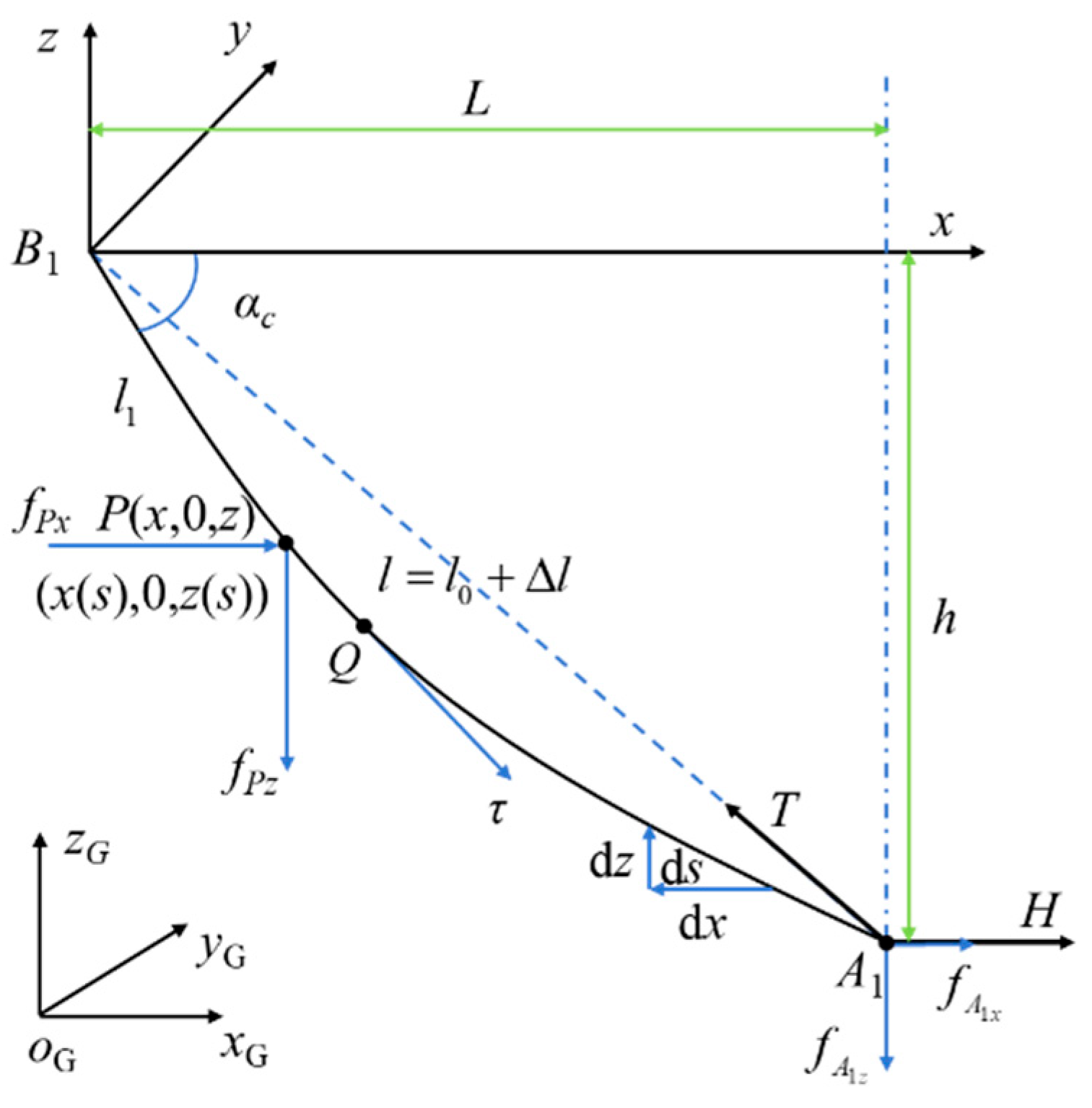
2.2. Static Modelling Based on Elastic Deformation of Slings

With the development of large-scale, heavy-duty lifting objects with uneven mass geometric structures in offshore engineering, DMP anti-swing control, which is typical of wind turbine blades, towers, containers, and shipwrecks, has attracted the attention of researchers. Meanwhile, considering that, in high-altitude lifting operations, the lifting cables for such loads are characterised by their long length, large span, and significant tensile strength, the self-weight and elastic deformation problem of the slings cannot be ignored. Therefore, static modelling of the flexible cable parallel anti-swing system in the equilibrium state is carried out based on the completed kinematic model.

Since the four anti-swing cables in the marine crane flexible cable parallel anti-swing system are symmetrical in three-dimensional space, only one anti-swing cable is selected for the static modelling analysis. In addition, when the horizontal span of the anti-swing cable is large and the height difference is small, the anti-swing cable will generate obvious deformation due to the wind resistance and its own gravity, resulting in a catenary phenomenon. Therefore, the static catenary model of the anti-swing cable, considering its own gravity and elastic deformation, is shown in Figure 3. L is the horizontal span of the anti-swing cable, h is the height difference between the anti-swing cable connection points A₁ and B₁, α_c is the inclination angle of the anti-swing cable, and the anti-swing cable l₁ is located in the o_B–x_Bz_B plane. H is the horizontal component of the tension T of the anti-swing cable, and ds is the microelement of any length of the anti-swing cable.

The coordinates of any point P on the anti-swing cable located in the o–xy plane in Figure 3 are defined as (x, 0, z) (where 0 ≤ x ≤ L, 0 ≤ z ≤ h), and the cable tension at this point is f_p. When the stretching deformation of the anti-swing cable is not considered, the coordinates of point P are (x (s), 0, z (s)) (where 0 ≤ x (s) ≤ L, 0 ≤ z (s) ≤ h), and the relationship satisfied by the differential unit at any point P of the anti-swing cable is,

$${\left({\displaystyle \frac{\mathrm{d}x}{\mathrm{d}p}}\right)}^2+{\left({\displaystyle \frac{\mathrm{d}z}{\mathrm{d}p}}\right)}^2=1$$

(13)

$$f_P{\displaystyle \frac{\mathrm{d}x}{\mathrm{d}p}}=f_{Px}=f_{A_{1x}}$$

(14)

$$f_p{\displaystyle \frac{\mathrm{d}z}{\mathrm{d}p}}=f_{Pz}=f_{A_{1z}}-\rho g(l_0-s)$$

(15)

where, $f_{Px}$ is the component force of f_p on the x-axis and $f_{Pz}$ is the component force of f_p on the z-axis. $f_{A_1}$ is the tension force of the anti-swing cable at point A₁, $f_{A_{1x}}$ is the component force of $f_{A_1}$ on the x-axis, and $f_{A_{1z}}$ is the component force of $f_{A_1}$ on the z-axis.

According to Equations (13)–(15), the expression for the calculation of the tension at any point P of the anti-swing cable is obtained.

$$f_P=\sqrt{f_{Px}^2+f_{Pz}^2}=\sqrt{f_{A_{1x}}^2+{(f_{A_{1z}}-\rho g(l_0-s))}^2}$$

(16)

Furthermore, according to Hooke’s law, the force at point P is $f_P$, so,

$$f_P=E{S}_0\left({\displaystyle \frac{\mathrm{d}l}{\mathrm{d}{l}_0}}-1\right)=E{S}_0\left({\displaystyle \frac{\mathrm{d}p}{\mathrm{d}s}}-1\right)$$

(17)

Using the differential formula ${\displaystyle \frac{\mathrm{d}x}{\mathrm{d}s}}={\displaystyle \frac{\mathrm{d}x}{\mathrm{d}p}}{\displaystyle \frac{\mathrm{d}p}{\mathrm{d}s}}$ and ${\displaystyle \frac{\mathrm{d}z}{\mathrm{d}s}}={\displaystyle \frac{\mathrm{d}z}{\mathrm{d}p}}{\displaystyle \frac{\mathrm{d}p}{\mathrm{d}s}}$, Equations (14)–(17) can be rewritten as follows:

$${\displaystyle \frac{\mathrm{d}x}{\mathrm{d}s}}={\displaystyle \frac{f_{A_{1x}}}{E{S}_0}}+{\displaystyle \frac{f_{A_{1x}}}{\sqrt{f_{A_{1x}}^2+{(f_{A_{1z}}-\rho g(l_0-s))}^2}}}$$

(18)

$${\displaystyle \frac{\mathrm{d}z}{\mathrm{d}s}}=(f_{A_{1z}}-\rho g(l_0-s))\left({\displaystyle \frac{1}{E{S}_0}}+{\displaystyle \frac{1}{\sqrt{f_{A_{1x}}^2+{(f_{A_{1z}}-\rho g(l_0-s))}^2}}}\right)$$

(19)

Further, Equations (18) and (19) are integrated respectively.

$$x(s)={\displaystyle {\int }_0^s\frac{\mathrm{d}x}{\mathrm{d}s}\mathrm{d}s=\frac{f_{A_{1x}}s}{E{S}_0}+\frac{\left|f_{A_{1x}}\right|}{\rho g}\ln \left(\frac{f_{A_{1z}}-\rho g(l_0-s)+\sqrt{f_{A_{1x}}^2+{(f_{A_{1z}}-\rho g(l_0-s))}^2}}{f_{A_{1z}}-\rho g{l}_0+\sqrt{f_{A_{1x}}^2+{(f_{A_{1z}}-\rho g{l}_0)}^2}}\right)}$$

(20)

$$\begin{array}{l}z(s)={\displaystyle {\int }_0^s\frac{\mathrm{d}z}{\mathrm{d}s}\mathrm{d}s=}{\displaystyle \frac{2f_{A_{1z}}s-\rho g(2l_{0}s-s^2)}{2E{S}_0}}+\sqrt{f_{A_{1x}}^2+{(f_{A_{1z}}-\rho g(l_0-s))}^2}-\sqrt{f_{A_{1x}}^2+{(f_{A_{1z}}-\rho g{l}_0)}^2}\\ -{\displaystyle \frac{\left|\rho g{l}_0-f_{A_{1z}}+l_0\right|}{\rho g}}\ln \left({\displaystyle \frac{f_{A_{1z}}-\rho g(l_0-s)+\sqrt{f_{A_{1x}}^2+{(f_{A_{1z}}-\rho g(l_0-s))}^2}}{f_{A_{1z}}-\rho g{l}_0+\sqrt{f_{A_{1x}}^2+{(f_{A_{1z}}-\rho g{l}_0)}^2}}}\right)\end{array}$$

(21)

Then, the formula for calculating the length l of the anti-swing cable is as follows:

$$l={\displaystyle {\int }_0^{l_0}\sqrt{{\left(\frac{f_{A_{1x}}}{\sqrt{f_{A_{1x}}^2+{(f_{A_{1z}}-\rho g{l}_0+\rho gs)}^2}}+\frac{f_{A_{1x}}}{E{S}_0}\right)}^2+{\left(\begin{array}{l}\frac{f_{A_{1z}}-\rho g{l}_0+\rho gs}{\sqrt{f_{A_{1x}}^2+{(f_{A_{1z}}-\rho g{l}_0+\rho gs)}^2}}\\ +\frac{f_{A_{1z}}-\rho g{l}_0+\rho gs}{E{S}_0}\end{array}\right)}^2}\mathrm{d}s}$$

(22)

Afterwards, by substituting s = l₀ in Equations (20) and (21), the coordinates of point A₁ can be obtained:

$$x_{A_1}={\displaystyle \frac{f_{A_{1x}}{l}_0}{E{S}_0}}+{\displaystyle \frac{\left|f_{A_{1x}}\right|}{\rho g}}\ln \left({\displaystyle \frac{f_{A_{1z}}+f_{A_1}}{f_{A_{1z}}-\rho g{l}_0+\sqrt{f_{A_{1x}}^2+{(f_{A_{1z}}-\rho g{l}_0)}^2}}}\right)$$

(23)

$$z_{A_1}={\displaystyle \frac{2f_{A_{1z}}{l}_0-\rho g{l}_0^2}{2E{S}_0}}+f_{A_1}-\sqrt{f_{A_{1x}}^2+{(f_{A_{1z}}-\rho g{l}_0)}^2}-{\displaystyle \frac{\left|\rho g{l}_0-f_{A_{1z}}+l_0\right|}{\rho g}}\ln \left({\displaystyle \frac{f_{A_{1z}}+f_{A_1}}{f_{A_{1z}}-\rho g{l}_0+\sqrt{f_{A_{1x}}^2+{(f_{A_{1z}}-\rho g{l}_0)}^2}}}\right)$$

(24)

In this way, the expressions for the anti-swing cable tension $f_{A_i}$ and the original rope length l₀ are obtained. In addition, the equation for the angle of inclination of the anti-swing cable can be obtained from Equations (23) and (24).

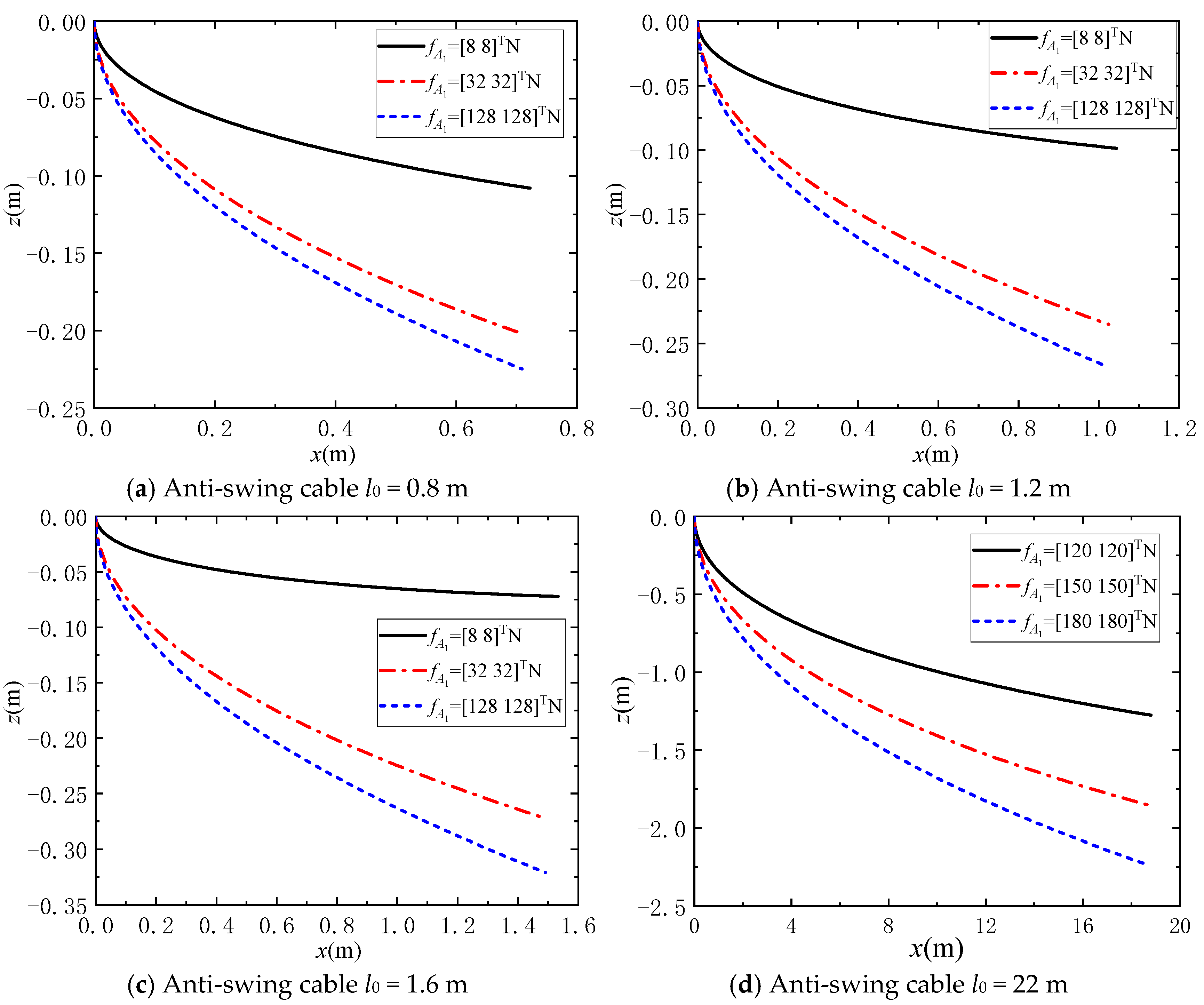
2.3. Static Analysis of Anti-Swing Cable Catenary Model

Under the influence of various marine environmental excitations and unknown disturbances, the payload in the flexible cable parallel anti-swing system will swing. Therefore, a static analysis of the catenary model of the anti-swing cable in the flexible cable parallel anti-swing system of the marine crane is carried out. The parameter information of the anti-swing cable is presented in

Table 1. Parameter details of the anti-swing cables.

Symbol	Parameter Values
Elastic modulus E/Gpa	20
Cable diameter d/m	3 × 10−3
Cross-sectional area without elastic deformation S0/m2	7.069 × 10−4
Line density without deformation ρ/kg m	0.065

. The initial tension values of the anti-swing cable are f_A1 = [f_A1x f_A1y]^T = [8 8]^TN, f_A1 = [f_A1x f_A1y]^T = [32 32]^TN, and f_A1 = [f_A1x f_A1y]^T = [128 128]^TN, respectively.

Equations (20) and (21) are then used to calculate the natural state of the anti-swing cables of different lengths under different initial tension forces. At the same time, Mathematica 12.0 software is used to calculate Equation (22) to obtain the cable length l of the anti-swing cable under tension. Finally, a static characteristic analysis is carried out on the established model of the anti-swing cable catenary, and the results are as follows:

By analysing Figure 4a–d, it can be seen that, as the horizontal span of the cable becomes significantly larger when the marine crane is lifting a large payload, the lifting cable is prone to catenary phenomenon. In the study of the catenary static simulation of an anti-swing cable with different initial lengths and tension groups, for a fixed anti-swing cable length, the inclination angle gradually increases as the given tension increases. The catenary model of the anti-swing cable more effectively illustrates the cable’s contour under its own gravity and external forces, and the cable is pulled straighter as the tension increases. At the same time, the catenary characteristics of the anti-swing cable are not very clear in the first three simulation groups. In the fourth group, when the length of the anti-swing cable becomes 22 m, the contour characteristics of the anti-swing cable in space become relatively obvious, the elongation of the anti-swing cable Δl changes more obviously, and the chord length error of the anti-swing cable also reaches 14.95%.

3. Dynamic Modelling of Diversified Lifting Operations for Flexible Cable Parallel Anti-Swing System

Unlike the onshore crane lifting of DMP, the ship will be affected by rolling, pitching, yawing, swaying, surging, and heaving during the DMP lifting operation at sea, especially by rolling and pitching. These excitations transmit through the ship to the crane, causing the DMP to swing in three dimensions and endangering the safety and efficiency of offshore lifting operations. Therefore, the coupled dynamic equations of the ship, crane, and DMP system under roll, pitch excitation, and random disturbance are derived in this section.

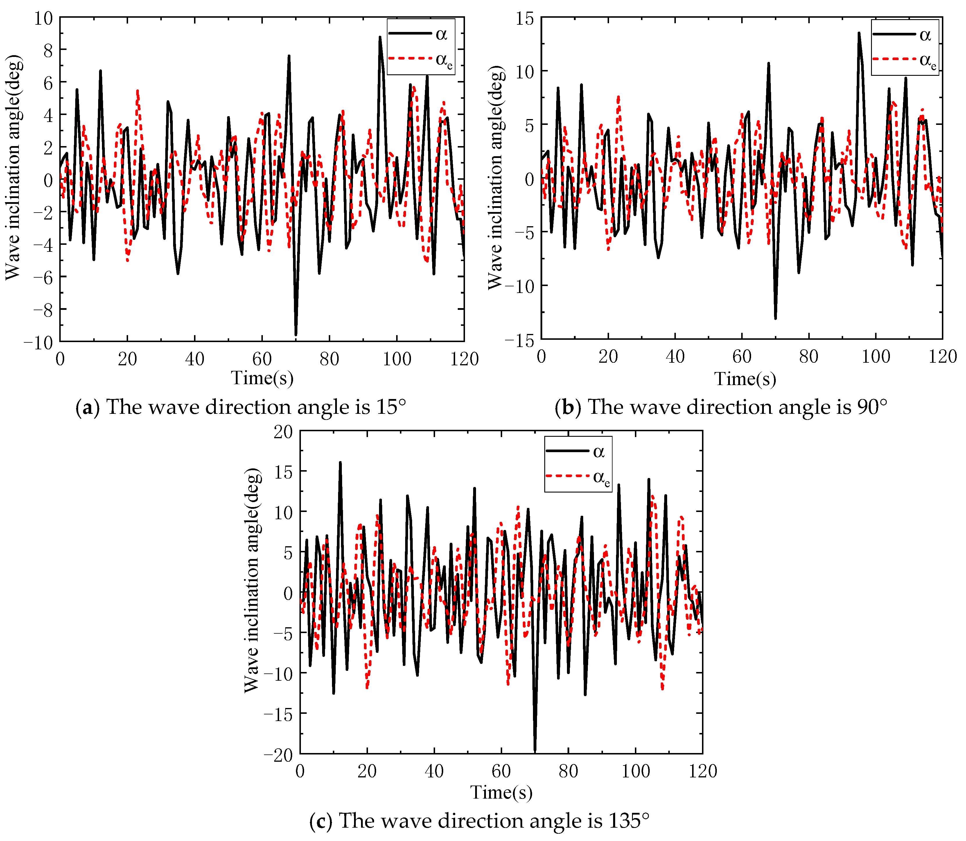
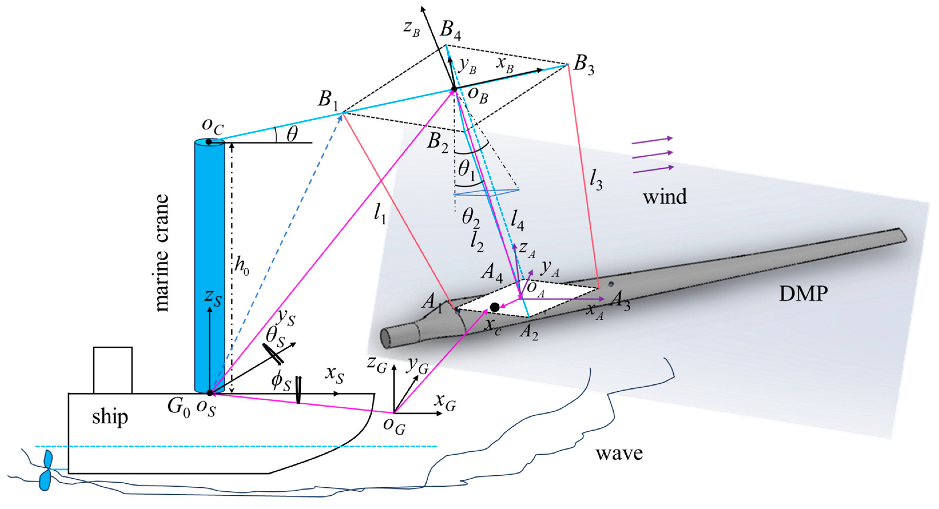
3.1. Ship Roll and Pitch Coupling Motion Modelling

In Figure 5, the coordinate system of the ship in the static environment is o–xyz, the coordinate system under rolling and pitching excitation is O₀–X₀Y₀Z₀, the centre of gravity of the ship is G₀, and the coordinate system origin o and O₀ coincide with the centre of gravity G₀. In deriving the coupled motion equations of the ship under rolling and pitching excitation, the following assumptions are made.

(1)

Ignoring the influence of yaw on the ship motion, the angular displacement and angular velocity of yaw are both 0.

(2)

The centre of gravity position G₀ is fixed under the coupled excitation of roll and pitch.

(3)

Both ship roll and pitch occur around the centre of gravity, point G₀.

According to the coordinate transformation rules in robotics, the coordinates of a ship in the O₀–X₀Y₀Z₀ coordinate system can be expressed as follows:

$$\left[\begin{array}{c}{X}_0\\ Y_0\\ Z_0\end{array}\right]=R\left[\begin{array}{c}x\\ y\\ z\end{array}\right]$$

(25)

where, $R=\left[\begin{array}{ccc}\cos {\theta }_S& 0& \sin {\theta }_S\\ 0& 1& 0\\ -\sin {\theta }_S& 0& \cos {\theta }_S\end{array}\right]\left[\begin{array}{ccc}1& 0& 0\\ 0& \cos {\varphi }_S& -\sin {\varphi }_S\\ 0& \sin {\varphi }_S& \cos {\varphi }_S\end{array}\right]$.

The roll and pitch angular velocities of a ship are as follows:

$$\left[\begin{array}{c}{\omega }_{X_0}\\ {\omega }_{Y_0}\\ {\omega }_{Z_0}\end{array}\right]=R\left[\begin{array}{c}{\omega }_x\\ {\omega }_y\\ 0\end{array}\right]=\left[\begin{array}{c}\cos {\theta }_S\left({\displaystyle \frac{d{\varphi }_S}{dt}}\right)+\sin {\theta }_S\sin {\varphi }_S\left({\displaystyle \frac{d{\theta }_S}{dt}}\right)\\ \cos {\varphi }_S\left({\displaystyle \frac{d{\theta }_S}{dt}}\right)\\ -\sin {\theta }_S\left({\displaystyle \frac{d{\varphi }_S}{dt}}\right)+\cos {\theta }_S\sin {\varphi }_S\left({\displaystyle \frac{d{\theta }_S}{dt}}\right)\end{array}\right]$$

(26)

where, ${\omega }_x=d{\varphi }_S/dt$, ${\omega }_y=d{\theta }_S/dt$, ${\omega }_z=0$.

Due to the structural symmetry of ships along the longitudinal axis (ox axis) and in the vertical direction (oz axis), the mass distribution of the ship is relatively uniform. According to the definition formula of the moment of inertia $J={\displaystyle \int r^{2}dm}$ (where r is the perpendicular distance from the mass element dm to the rotation axis), it is known that the integration of the mass distribution and distance to the axis of ships on the ox and oz axes is similar, which implies that J_x = J_z. Thus, the kinetic energy expression T of the ship under the coupled excitation of roll and pitch is as follows:

$$T={\displaystyle \frac{1}{2}}{J}_x{\omega }_{X_0}^2+{\displaystyle \frac{1}{2}}{J}_y{\omega }_{Y_0}^2+{\displaystyle \frac{1}{2}}{J}_z{\omega }_{Z_0}^2={\displaystyle \frac{1}{2}}{J}_x\left({\left({\displaystyle \frac{d{\varphi }_S}{dt}}\right)}^2+{\left(\sin {\varphi }_S\left({\displaystyle \frac{d{\theta }_S}{dt}}\right)\right)}^2\right)+{\displaystyle \frac{1}{2}}{J}_y{\left(\cos {\varphi }_S\left({\displaystyle \frac{d{\theta }_S}{dt}}\right)\right)}^2$$

(27)

where J_x, J_y, and J_z are the moments of inertia of the ship about the o_x, o_y, and o_z, respectively.

The calculation of potential energy is usually based on the work done by the force. For conservative forces, the change in potential energy is equal to the negative work done by the conservative force, which means V = −W, where V is the potential energy and W is the work done by the force. In the ship system, it mainly involves gravity and restoring moment. According to the previous assumption, it can be seen that the centre of gravity position of the ship is unchanged, meaning that the work done by gravity is 0, while the work done by the restoring moment will cause a change in the potential energy. Therefore, in the coupled environment of roll and pitch, when the roll and pitch angles of the ship are large, the stability of the ship changes from initial stability to large inclination stability. Therefore, the restoring moments obtained by calculating the equations are as follows:

$$\left\{\begin{array}{c}{M}_x=\rho \nabla gGM\sin {\varphi }_S\\ M_y=\rho \nabla gGN\sin {\theta }_S\end{array}\right.$$

(28)

where ρ is the density of seawater, ▽ is the displacement of the ship, g is the acceleration due to gravity, GM is the metacentric height of the ship in roll, and GN is the metacentric height of the ship in pitch.

The total potential energy of the ship system is as follows:

$$\begin{array}{l}V=-{\displaystyle {\int }_0^{{\varphi }_S}\rho \nabla gGM\sin {\varphi }_{S}d{\varphi }_S}-{\displaystyle {\int }_0^{{\theta }_S}\rho \nabla gGN\sin {\theta }_{S}d{\theta }_S}\\ =\rho \nabla gGM\cos {\varphi }_S-\rho \nabla gGM+\rho \nabla gGN\cos {\theta }_S-\rho \nabla gGN\end{array}$$

(29)

When the swing angle of a ship is small, it can generally be assumed that the damping torque and angular velocity are linearly related, but the roll and pitch of a ship are often nonlinear. Therefore, a nonlinear term containing square terms and sign functions is introduced here to describe the nonlinear damping effect caused by various complex fluid dynamic effects in the roll and pitch process, as follows:

$$M_{{\varphi }_S}=2N_{{\varphi }_S}{\displaystyle \frac{d{\varphi }_S}{dt}}-{\lambda }_r{J}_x{\left({\displaystyle \frac{d{\varphi }_S}{dt}}\right)}^2\mathrm{sgn}\left({\displaystyle \frac{d{\varphi }_S}{dt}}\right)$$

(30)

$$M_{{\theta }_S}=2N_{{\theta }_S}{\displaystyle \frac{d{\theta }_S}{dt}}-{\lambda }_p{J}_y{\left({\displaystyle \frac{d{\theta }_S}{dt}}\right)}^2\mathrm{sgn}\left({\displaystyle \frac{d{\theta }_S}{dt}}\right)$$

(31)

where $N_{{\varphi }_S}$ and $N_{{\theta }_S}$ are the roll and pitch damping coefficients of the ship, respectively, which are dimensionless coefficients. λ_r and λ_p are coefficients related to the damping characteristics of ship roll and pitch, respectively, and $\mathrm{sgn}\left({\displaystyle \frac{d{\varphi }_S}{dt}}\right)$ and $\mathrm{sgn}\left({\displaystyle \frac{d{\theta }_S}{dt}}\right)$ are the sign function.

$$\mathrm{sgn}\left({\displaystyle \frac{d{\varphi }_S}{dt}}\right)=\left\{\begin{array}{cc}1& {\displaystyle \frac{d{\varphi }_S}{dt}}>0\\ -1& {\displaystyle \frac{d{\varphi }_S}{dt}}<0\end{array}\right., \mathrm{sgn}\left({\displaystyle \frac{d{\theta }_S}{dt}}\right)=\left\{\begin{array}{cc}1& {\displaystyle \frac{d{\theta }_S}{dt}}>0\\ -1& {\displaystyle \frac{d{\theta }_S}{dt}}<0\end{array}\right.$$

The positive and negative signs are used to indicate the direction of the roll and pitch angular velocities, ensuring that the direction of the nonlinear damping moment is consistent with the actual process.

According to Hamilton’s variational principle, it is known that the work done by the non-conservative forces in the coupled rolling and pitching motion of a ship is also an indispensable part of the process. When marine cranes lift a DMP, the ship also encounters the ocean current interference force, causing the ship to swing, which is mainly affected by the wave force exerted on the outer surface of the ship by the fluid around the hull. The wave force is usually divided into drag force and inertia force. It is also assumed that the ship is in a static state, which ignores the influence of the inertial force and only considers the wave force generated by the drag force. Here, Morison’s formula is used to obtain the calculation method of the ship’s drag force, and then the calculation formula of the wave moment is as follows [34].

$$M_x=-\psi \left({\displaystyle \frac{1}{240}}{\displaystyle \frac{\rho C_{Dx}{({\omega }_x\cos {\theta }_S)}^3{b}^5}{\sin {\varphi }_S\sin {\theta }_S{\omega }_x+\cos {\varphi }_S{\omega }_y}}+{\displaystyle \frac{1}{48}}\rho C_{Dx}(\sin {\varphi }_S\sin {\theta }_S{\omega }_x+\cos {\varphi }_S{\omega }_y)\cos {\theta }_S{\omega }_x{L}^2{b}^3\right)$$

(32)

$$M_y=-{\psi }_1\left(\begin{array}{l}{\displaystyle \frac{1}{960}}{\displaystyle \frac{\rho C_{Dy}{({\omega }_x\cos {\theta }_S)}^4{b}^5}{{(\sin {\varphi }_S\sin {\theta }_S{\omega }_x+\cos {\varphi }_S{\omega }_y)}^2}}-\\ {\displaystyle \frac{1}{64}}\rho C_{Dy}{(\sin {\varphi }_S\sin {\theta }_S{\omega }_x+\cos {\varphi }_S{\omega }_y)}^2{L}^{4}b\end{array}\right)-{\displaystyle \frac{1}{96}}\rho C_{Dy}{({\omega }_x\cos {\theta }_S)}^2{L}^2{b}^3$$

(33)

where C_Dx and C_Dy are the drag force coefficients of the ship in the direction of the x and y axes, respectively, in the static coordinate system o–xyz. L and b are the equivalent length and width, respectively, of the ship’s hull projected onto the water surface.

Assuming that the ship is subjected to regular waves during the DMP lifting operation at sea, the motion of the ship is actually a “resultant force of effective wave surfaces” of roll and pitch. In other words, the ship is subjected to the effective wave inclination ${\alpha }_e$, and meets the ${\alpha }_e={\alpha }_{\omega e}\sin (\omega t+\varphi )$. Similarly, when calculating the disturbance moment of regular waves, the ship is assumed to be static. At this time, the ship’s gravity and buoyancy are equal, and it is perpendicular to the effective wave surface, maintaining the ship’s swing angle at π/12. Therefore, the restoring disturbance moment composed of gravity and buoyancy during the roll and pitch motion of a ship can be expressed as follows:

$$M_{X_0}=\rho \nabla gGM{\alpha }_{e1}\sin \left({\displaystyle \frac{\pi }{12}}\sin ({\Omega }_{1}t+{\varphi }_1)\right)$$

(34)

$$M_{Y_0}=\rho \nabla gGN{\alpha }_{e2}\sin \left({\displaystyle \frac{\pi }{12}}\sin ({\Omega }_{2}t+{\varphi }_2)\right)$$

(35)

where, Ω₁ and Ω₂ are the wave excitation frequencies for the ship’s roll and pitch motion, respectively. ϕ₁ and ϕ₂ are the initial phase angles for the ship’s roll and pitch excitations, respectively.

Next, based on the Hamilton variational principle, the work done by the non-conservative forces of the ship system under roll and pitch excitation is calculated. The Hamilton variational principle is as follows [35]: Given the initial and final states of the system, its true motion is such that the time integral of the Lagrange quantity L reaches its minimum value. The Lagrange quantity L is usually expressed as L (q, q̇, t), where q is the generalised coordinate, q̇ is the generalised velocity, and t is the time.

$${\displaystyle {\int }_{t_1}^{t_2}\left(\delta L+{\displaystyle \sum _i{Q}_i\delta q_i}\right)}dt=0$$

(36)

where $\delta L$ is the variation of the Lagrange operator L of the system, and L = T − V denotes a small change in the combined kinetic and potential energy state of the system. ${\displaystyle \sum _i{Q}_i\delta q_i}$ is the virtual work done by all the non-conservative forces in the ship system, which in this case mainly refers to the work done by the wave force and wind resistance. Q_i is the generalised force corresponding to the generalised coordinates.

Combining (27) and (29), we obtain the expression for the Lagrange function of the system:

$$\begin{array}{l}L={\displaystyle \frac{1}{2}}{J}_x\left({\left({\displaystyle \frac{d{\varphi }_S}{dt}}\right)}^2+{\left(\sin {\varphi }_S\left({\displaystyle \frac{d{\theta }_S}{dt}}\right)\right)}^2\right)+{\displaystyle \frac{1}{2}}{J}_y{\left(\cos {\varphi }_S\left({\displaystyle \frac{d{\theta }_S}{dt}}\right)\right)}^2-\\ \rho \nabla gGM\cos {\varphi }_S+\rho \nabla gGM-\rho \nabla gGN\cos {\theta }_S+\rho \nabla gGN\end{array}$$

(37)

Then, by substituting Equations (30)–(35) and (37) into Equation (36), the coupled motion equations of the ship under rolling and pitching excitation are obtained as follows:

$$\begin{array}{l}{\left({\displaystyle \frac{d{\varphi }_S}{dt}}\right)}^2+{\displaystyle \frac{\left(\begin{array}{l}\rho \nabla gGM\sin {\varphi }_S+2N_{{\varphi }_S}\frac{d{\varphi }_S}{dt}-{\lambda }_r{J}_x{\left(\frac{d{\varphi }_S}{dt}\right)}^2\mathrm{sgn}\left(\frac{d{\varphi }_S}{dt}\right)-\\ \psi \cos {\theta }_S\left(\frac{1}{240}\frac{\rho C_{Dx}{(\frac{d{\varphi }_S}{dt}\cos {\theta }_S)}^3{b}^5}{\frac{d{\varphi }_S}{dt}\sin {\varphi }_S\sin {\theta }_S+\frac{d{\theta }_S}{dt}\cos {\varphi }_S}+\frac{\cos {\theta }_S{L}^2{b}^3}{48}\frac{d{\varphi }_S}{dt}\rho C_{Dx}(\frac{d{\varphi }_S}{dt}\sin {\varphi }_S\sin {\theta }_S+\frac{d{\theta }_S}{dt}\cos {\varphi }_S)\right)-\\ {\psi }_1\left(\begin{array}{l}\frac{1}{960}\frac{\rho C_{Dy}{(\frac{d{\varphi }_S}{dt}\cos {\theta }_S)}^4{b}^5}{{(\frac{d{\varphi }_S}{dt}\sin {\varphi }_S\sin {\theta }_S+\frac{d{\theta }_S}{dt}\cos {\varphi }_S)}^2}-\\ \frac{1}{64}\rho C_{Dy}{(\frac{d{\varphi }_S}{dt}\sin {\varphi }_S\sin {\theta }_S+\frac{d{\theta }_S}{dt}\cos {\varphi }_S)}^2{L}^{4}b-\frac{1}{96}\rho C_{Dy}{(\frac{d{\varphi }_S}{dt}\cos {\theta }_S)}^2{L}^2{b}^3\end{array}\right)\left(\begin{array}{l}{\varphi }_S\cos {\varphi }_S\sin {\theta }_S+\\ \sin {\varphi }_S\sin {\theta }_S-{\theta }_S\sin {\varphi }_S\end{array}\right)\end{array}\right)}{J_x{\left(\sin {\varphi }_S\left(\frac{d{\theta }_S}{dt}\right)\right)}^2+J_y{\left(\cos {\varphi }_S\left(\frac{d{\theta }_S}{dt}\right)\right)}^2}}\\ ={\displaystyle \frac{\rho \nabla gGM{E}_1\sin \left(\frac{\pi }{12}\sin ({\mathsf{\Omega }}_{1}t+{\varphi }_1)\right)}{J_x{\left(\sin {\varphi }_S\left(\frac{d{\theta }_S}{dt}\right)\right)}^2+J_y{\left(\cos {\varphi }_S\left(\frac{d{\theta }_S}{dt}\right)\right)}^2}}\end{array}$$

(38)

$$\begin{array}{l}{\left({\displaystyle \frac{d{\theta }_S}{dt}}\right)}^2+{\displaystyle \frac{1}{J_y}}\left(\begin{array}{l}\rho \nabla gGN\sin {\theta }_S+2{\displaystyle \frac{d{\theta }_S}{dt}}{N}_{{\theta }_S}-{\lambda }_p{J}_y{\left({\displaystyle \frac{d{\theta }_S}{dt}}\right)}^2\mathrm{sgn}\left({\displaystyle \frac{d{\theta }_S}{dt}}\right)\\ +(J_y-J_x)\sin {\theta }_S\cos {\theta }_S{\left({\displaystyle \frac{d{\varphi }_S}{dt}}\right)}^2\end{array}\right)+\\ {\displaystyle \frac{\psi }{J_y}}\left({\displaystyle \frac{1}{240}}{\displaystyle \frac{\rho C_{Dx}{(\frac{d{\varphi }_S}{dt}\cos {\theta }_S)}^3{b}^5}{\frac{d{\varphi }_S}{dt}\sin {\varphi }_S\sin {\theta }_S+\frac{d{\theta }_S}{dt}\cos {\varphi }_S}}+{\displaystyle \frac{\cos {\theta }_S{L}^2{b}^3}{48}}{\displaystyle \frac{d{\varphi }_S}{dt}}\rho C_{Dx}({\displaystyle \frac{d{\varphi }_S}{dt}}\sin {\varphi }_S\sin {\theta }_S+{\displaystyle \frac{d{\theta }_S}{dt}}\cos {\varphi }_S)\right){\varphi }_S\sin {\theta }_S-\\ \left(\begin{array}{l}{\displaystyle \frac{{\psi }_1}{J_y}}\left(\begin{array}{l}{\displaystyle \frac{1}{960}}{\displaystyle \frac{\rho C_{Dy}{(\frac{d{\varphi }_S}{dt}\cos {\theta }_S)}^4{b}^5}{{(\frac{d{\varphi }_S}{dt}\sin {\varphi }_S\sin {\theta }_S+\frac{d{\theta }_S}{dt}\cos {\varphi }_S)}^2}}-\\ {\displaystyle \frac{1}{64}}\rho C_{Dy}{({\displaystyle \frac{d{\varphi }_S}{dt}}\sin {\varphi }_S\sin {\theta }_S+{\displaystyle \frac{d{\theta }_S}{dt}}\cos {\varphi }_S)}^2{L}^{4}b\end{array}\right)-\\ {\displaystyle \frac{1}{96}}\rho C_{Dy}{({\displaystyle \frac{d{\varphi }_S}{dt}}\cos {\theta }_S)}^2{L}^2{b}^3\end{array}\right)\left({\varphi }_S\sin {\varphi }_S\cos {\theta }_S+\cos {\varphi }_S\right)={\displaystyle \frac{\rho \nabla gGN{E}_2\sin \left(\frac{\pi }{12}\sin ({\mathsf{\Omega }}_{2}t+{\varphi }_2)\right)}{J_y}}\end{array}$$

(39)

In this way, the mathematical modelling of the coupled motion of the ship’s roll and pitch is completed. At the same time, considering the complexity of solving the motion equation of the above-mentioned ship under the coupled excitation of roll and pitch, the fourth-order Runge–Kutta method is used to solve it. Taking the scientific ship “YUKUN” of Dalian Maritime University as an example for lifting simulation research, the relevant parameters are shown in

Table 2. Main parameters of the “YuKun” ship.

Parameter	Value	Parameter	Value
L	116 m	B	18 m
D	8.35 m	d	5.4 m
▽	5710.2 m3	GM	1.71 m
GN	4.93 m	KG	6.45 m
ω1	0.607 rad/s	ω2	0.562 rad/s

[36].

When the marine crane is used for lifting operations at sea, the ship is actually in a static environment. Therefore, taking the ship’s speed as 0 kn, the simulation analysis of the wave inclination angle, roll angle, and pitch angle is carried out under the wave direction angle of 15°, 90° and 135°, respectively, and the results are shown in Figure 6a–c. As can be seen from Figure 6a–c, as the wave direction angle increases, the ship’s effective wave inclination angle under the coupled action of roll and pitch also increases also increases, and the excitation effect on the ship is also enhanced. It can be seen from Figure 7a–c that, as the wave direction angle increases, the ship’s roll and pitch angles also increase.

3.2. DMP Dynamic Modelling of Flexible Cable Parallel Anti-Swing System

Taking the flexible cable parallel anti-swing system lifting distributed mass blades as an example, the whole lifting process can be divided into lifting and suspending processes, as shown in Figure 8. Additionally, the lifting cable will change from a relaxed state to a tensioned state during the lifting process. In the above three lifting processes, which are affected by the special geometric structure and mass distribution of the payload, the horizontal span of the lifting cable is larger, which may cause the overhanging phenomenon of the lifting cable, thus posing challenges to the control of the payload anti-swing and attitude adjustment. Therefore, it is necessary to model the catenary of the cable. Due to the influence of ship roll and pitch, the DMP may experience instability and swing during the lifting stage. To solve the above problems, motion compensation systems, mechanical assistance, and manual pulling of auxiliary cables are used in practical engineering to suppress the swing of the DMP. Therefore, the motion of the DMP can be ignored during the lifting process. However, the DMP needs to carry out swing suppression and maintain the crane posture during the suspension process under the influence of roll, pitch, wind loads, and other known/unknown disturbances.

In the suspension process of the flexible cable parallel anti-swing system of the marine crane for lifting the DMP, the DMP is suspended below the end of the crane boom structure by the main sling and anti-swing cables. The hoisting cable is tensioned and may even be slightly deformed; it will vibrate transversely under the disturbance of the external wind. Payload will swing under the excitation of the marine environment, and, even due to improper hoisting, torsional instability may occur, thus breaking the static attitude and position maintained under static balance.

The horizontal lifting of a single DMP is analysed here. For a payload with a regular shape and uniform mass distribution, its centre of gravity coincides with the centre of the geometric structure. For a wind turbine blade with uneven mass distribution and irregular geometric structure, its centre of gravity is generally distributed on the side where the geometric centre of the blade is close to the blade root. Here, the principle of moment balance in physics is used to calculate and obtain the position coordinates of the centre of mass of the blade, and then to obtain the results of the position of the centre of the wind turbine blade. Specifically, assuming that the wind turbine blade is divided into n small regular mass particles, the mass of each mass particle is m_i, the horizontal and vertical coordinates of each mass particle are x_i and y_i,, respectively, and the centre of gravity coordinates of the blade are (x_c, y_c), then the calculation process of the centre of gravity of the wind turbine blade is as follows:

$$x_c={\displaystyle \frac{{\displaystyle \sum _{i=1}^n{m}_i{x}_i}}{{\displaystyle \sum _{i=1}^n{m}_i}}}={\displaystyle \frac{{\displaystyle {\int }_1^n\rho x_{i}dx}}{m_p}}$$

(40)

$$y_c={\displaystyle \frac{{\displaystyle \sum _{i=1}^n{m}_i{y}_i}}{{\displaystyle \sum _{i=1}^n{m}_i}}}={\displaystyle \frac{{\displaystyle {\int }_1^n\rho y_{i}dy}}{m_p}}$$

(41)

where ρ is the mass density function of the wind turbine blade (kg/m), m_p is the total mass of a single wind turbine blade (kg), x_i is the blade length and $x_i\ll L$, y_i is the chord length of the blade l_max and $y_i\ll l_{\max }$, m; L is the total length of the wind turbine blade (m).

The fitted formula for the centre of gravity x_c of a wind turbine blade is $x_c=0.362L$. Therefore, the centre of gravity of the wind turbine blade is approximately one third of the blade root end.

$$y(x)=l_{\max }\left(2.69{\left({\displaystyle \frac{x}{L}}\right)}^3-5.07{\left({\displaystyle \frac{x}{L}}\right)}^2+1.89\left({\displaystyle \frac{x}{L}}\right)+0.63\right)$$

(42)

It is assumed that the blade is a rod-shaped model and that its mass distribution is only affected by the shape of the blade. Therefore, the blade moment of inertia derived based on the parallel axis theorem is given by,

$$I=I_c+M{\left({\displaystyle \frac{L}{2}}-{\displaystyle \frac{L}{3}}\right)}^2={\displaystyle \frac{m_p{L}^2}{9}}$$

(43)

For a payload with a regular shape and uniform mass distribution, it can be regarded as a rod-shaped payload, and its moment of inertia is $I=m_p{L}^2/12$.

Since the centre of gravity x_c and the geometric centre of gravity x₀ of the wind turbine blades do not coincide, there may be potential instability and rotation phenomenon of the blades during the suspension and transfer process, as shown in Figure 9, which is a schematic diagram of its static analysis. If the counterclockwise rotation direction is defined as positive, then on the o_A–x_Ay_A plane,

$$\left(F_m{r}_3\cos {\alpha }_m+F_1{r}_3\cos {\alpha }_1-F_2{r}_4\cos {\alpha }_2-F_3{r}_3\cos {\alpha }_3+F_4{r}_4\cos {\alpha }_4-F_w{r}_4\sin {\alpha }_0\right)={\displaystyle \frac{m_p{L}^2}{9}}{\displaystyle \frac{d\omega }{dt}}$$

(44)

where F_m is the main sling tension, and F₁, F₂, F₃ and F₄ are the anti-swing tensions. α_m, α₁, α₂, α₃ and α₄ are the angles between the main sling and the anti-swing cables l₁, l₂, l₃, and l₄, respectively, and the coordinate system o_A–x_Ay_Az_A on the x_Az_A plane.

In the vertical plane,

$$\left(\begin{array}{l}({}^{o_A}r_{o_A{x}_c}-{}^{G}r_{x_c})R^{\mathrm{T}}{F}_m\sin {\alpha }_m+m_{p}g{l}_{o_A{x}_c}+F_w{l}_{o_A{x}_c}\cos {\alpha }_0-F_1(l_{o_A{A}_1}-r_4)\sin {\alpha }_1+\\ F_2(l_{o_A{A}_2}-r_3)\sin {\alpha }_2+F_3(l_{o_A{A}_3}+r_4)\sin {\alpha }_3-F_4(l_{o_A{A}_4}+r_3)\sin {\alpha }_4\end{array}\right)=0$$

(45)

where $l_{x_c{x}_0}$ is the distance between the centre of gravity of the DMP and the centre of the geometric structure. The projections of the centre of gravity on the coordinate axes o_Ax_A and o_Ay_A are r₄ and r₃, respectively, and ω is the rotational angular velocity.

In Figure 10, ϕ_S and θ_S are the roll angle and pitch angle of the ship in the marine environment, respectively, and θ₁ and θ₂ are the in-plane (in the x_Bz_B plane) and out-of-plane (in the y_Bz_B plane) swing angles of the DMP, respectively. The crane base coordinate system coincides with the ship deck coordinate system, and the coordinates of points o_S, o_C, o_B, o_A, and x_c in the coordinate systems o_S–x_Sy_Sz_S, o_C–x_Cy_Cz_C and o_B -x_By_Bz_B are as follows, respectively:

$$\begin{array}{c}{}^{G}o_S={[\begin{array}{ccc}{x}_{o_S}\hfill & y_{o_S}\hfill & z_{o_S}\hfill \end{array}]}^{\mathrm{T}}, {}^{S}o_C={[\begin{array}{ccc}{x}_{o_C}& y_{o_C}& z_{o_C}\end{array}]}^T={[\begin{array}{ccc}{x}_{o_S}& y_{o_S}& z_{o_S}+h_0\end{array}]}^T\hfill \\ {}^{C}o_B={[\begin{array}{ccc}{x}_{o_B}& y_{o_B}& z_{o_B}\end{array}]}^{\mathrm{T}}={[\begin{array}{ccc}{x}_{o_C}+l_{o_C{o}_B}\cos \theta & y_{o_C}& z_{o_C}\end{array}+l_{o_C{o}_B}\sin \theta ]}^{\mathrm{T}}\hfill \\ {}^{B}o_A={[\begin{array}{ccc}{x}_{o_A}& y_{o_A}& z_{o_A}\end{array}]}^{\mathrm{T}}={[\begin{array}{ccc}{x}_{o_B}+l_{o_A{o}_B}\cos {\theta }_2\sin {\theta }_1& y_{o_B}-l_{o_A{o}_B}\sin {\theta }_2& z_{o_B}\end{array}-l_{o_B{o}_A}\cos {\theta }_2\cos {\theta }_1]}^{\mathrm{T}}\hfill \\ {}^{A}o_{x_c}={[\begin{array}{ccc}{x}_{o_C}& y_{o_C}& z_{o_C}\end{array}]}^{\mathrm{T}}={[\begin{array}{ccc}{x}_{o_A}-r_4& y_{o_A}-r_3& z_{o_A}\end{array}]}^{\mathrm{T}}\hfill \end{array}$$

Furthermore, based on the coordinate transformation principle and vector knowledge in robotics, the displacement vector ${}^{G}r_{x_c}$ of the centre of gravity coordinate x_c of the DMP relative to the inertial coordinate system o_G–x_Gy_Gz_G is obtained as follows:

$$\begin{array}{l}{}^{G}r_{x_c}={}^{G}r_{o_G{o}_S}+{}^{G}r_{o_S{o}_C}+{}^{G}r_{o_C{o}_B}+{}^{G}r_{o_B{o}_A}+{}^{G}r_{o_A{x}_c}=RT=\\ \left[\begin{array}{ccc}\cos {\theta }_S& 0& \sin {\theta }_S\\ 0& 1& 0\\ -\sin {\theta }_S& 0& \cos {\theta }_S\end{array}\right]\left[\begin{array}{ccc}1& 0& 0\\ 0& \cos {\varphi }_S& -\sin {\varphi }_S\\ 0& \sin {\varphi }_S& \cos {\varphi }_S\end{array}\right]\left[\begin{array}{c}{x}_{o_S}+l_{o_C{o}_B}\cos \theta +l_{o_A{o}_B}\cos {\theta }_2\sin {\theta }_1-r_4\\ y_{o_S}-l_{o_A{o}_B}\sin {\theta }_2-r_3\\ z_{o_S}+h_0+l_{o_C{o}_B}\sin \theta -l_{o_B{o}_A}\cos {\theta }_2\cos {\theta }_1\end{array}\right]\end{array}$$

(46)

where ${}^{G}r_{o_G{o}_S}$ is the displacement vector between o_S and o_G in the inertial coordinate system, ${}^{G}r_{o_S{o}_C}$ is the displacement vector between o_C and o_S in the inertial coordinate system, ${}^{G}r_{o_C{o}_B}$ is the displacement vector between o_B and o_C in the inertial coordinate system, and ${}^{G}r_{o_B{o}_A}$ is the displacement vector between o_A and o_B in the inertial coordinate system. ${}^{G}r_{o_A{x}_c}$ is the displacement vector between the centre of gravity x_C of the DMP and o_A in the inertial coordinate system.

Equation (46) is simplified as follows:

$${}^{G}r_{x_c}=\left[\begin{array}{l}\left(\begin{array}{l}(x_{o_S}+l_{o_C{o}_B}\cos \theta +l_{o_A{o}_B}\cos {\theta }_2\sin {\theta }_1-r_4)\cos {\theta }_S+(y_{o_S}-l_{o_A{o}_B}\sin {\theta }_2-\\ r_3)\sin {\theta }_S\sin {\varphi }_S+(z_{o_S}+h_0+l_{o_C{o}_B}\sin \theta -l_{o_B{o}_A}\cos {\theta }_2\cos {\theta }_1)\sin {\theta }_S\cos {\varphi }_S\end{array}\right)\hfill \\ \left((y_{o_S}-l_{o_A{o}_B}\sin {\theta }_2-r_3)\cos {\varphi }_S-(z_{o_S}+h_0+l_{o_C{o}_B}\sin \theta -l_{o_B{o}_A}\cos {\theta }_2\cos {\theta }_1)\sin {\varphi }_S\right)\hfill \\ \left(\begin{array}{l}-(x_{o_S}+l_{o_C{o}_B}\cos \theta +l_{o_A{o}_B}\cos {\theta }_2\sin {\theta }_1-r_4)\sin {\theta }_S+(y_{o_S}-l_{o_A{o}_B}\sin {\theta }_2-\\ r_3)\cos {\theta }_S\sin {\varphi }_S+(z_{o_S}+h_0+l_{o_C{o}_B}\sin \theta -l_{o_B{o}_A}\cos {\theta }_2\cos {\theta }_1)\cos {\theta }_S\cos {\varphi }_S\end{array}\right)\hfill \end{array}\right]$$

(47)

Taking the derivative of Equation (47), the result is as follows:

$${}^G\dot{r}_{x_c}=\left[\begin{array}{l}\left(\begin{array}{l}{\dot{l}}_{o_A{o}_B}\cos {\theta }_2\sin {\theta }_1\cos {\theta }_S+l_{o_A{o}_B}{\dot{\theta }}_1\cos {\theta }_1\cos {\theta }_2\cos {\theta }_S-l_{o_A{o}_B}{\dot{\theta }}_2\sin {\theta }_1\sin {\theta }_2\cos {\theta }_S-\\ (x_{o_S}+l_{o_C{o}_B}\cos \theta +l_{o_A{o}_B}\cos {\theta }_2\sin {\theta }_1-r_4){\dot{\theta }}_S\sin {\theta }_S+l_{o_A{o}_B}{\dot{\theta }}_1\cos {\theta }_2\sin {\theta }_1\sin {\theta }_S\cos {\varphi }_S-\\ l_{o_A{o}_B}{\dot{\theta }}_2\cos {\theta }_2\sin {\theta }_S\sin {\varphi }_S+(y_{o_S}-l_{o_A{o}_B}\sin {\theta }_2-r_3)({\dot{\theta }}_S\cos {\theta }_S\sin {\varphi }_S+{\dot{\varphi }}_S\sin {\theta }_S\cos {\varphi }_S)-\\ {\dot{l}}_{o_A{o}_B}\cos {\theta }_2\cos {\theta }_1\sin {\theta }_S\cos {\varphi }_S+l_{o_A{o}_B}{\dot{\theta }}_2\sin {\theta }_2\cos {\theta }_1\sin {\theta }_S\cos {\varphi }_S-{\dot{l}}_{o_A{o}_B}\sin {\theta }_2\sin {\theta }_S\sin {\varphi }_S\\ +(z_{o_S}+h_0+l_{o_C{o}_B}\sin \theta -l_{o_B{o}_A}\cos {\theta }_2\cos {\theta }_1)({\dot{\theta }}_S\cos {\theta }_S\cos {\varphi }_S-{\dot{\varphi }}_S\sin {\theta }_S\sin {\varphi }_S)\end{array}\right)\hfill \\ \left(\begin{array}{l}-{\dot{l}}_{o_A{o}_B}\sin {\theta }_2\cos {\varphi }_S-(y_{o_S}-l_{o_A{o}_B}\sin {\theta }_2-r_3){\dot{\varphi }}_S\sin {\varphi }_S+{\dot{l}}_{o_B{o}_A}\cos {\theta }_2\cos {\theta }_1\sin {\varphi }_S-\\ l_{o_B{o}_A}{\dot{\theta }}_2\sin {\theta }_2\cos {\theta }_1\sin {\varphi }_S-l_{o_B{o}_A}{\dot{\theta }}_1\cos {\theta }_2\sin {\theta }_1\sin {\varphi }_S-l_{o_A{o}_B}{\dot{\theta }}_2\cos {\theta }_2\cos {\varphi }_S-\\ (z_{o_S}+h_0+l_{o_C{o}_B}\sin \theta -l_{o_B{o}_A}\cos {\theta }_2\cos {\theta }_1){\dot{\varphi }}_S\cos {\varphi }_S\end{array}\right)\hfill \\ \left(\begin{array}{l}-{\dot{l}}_{o_A{o}_B}\cos {\theta }_2\sin {\theta }_1\sin {\theta }_S+l_{o_A{o}_B}{\dot{\theta }}_2\sin {\theta }_2\sin {\theta }_1\sin {\theta }_S-l_{o_A{o}_B}{\dot{\theta }}_1\cos {\theta }_2\cos {\theta }_1\sin {\theta }_S-\\ (x_{o_S}+l_{o_C{o}_B}\cos \theta +l_{o_A{o}_B}\cos {\theta }_2\sin {\theta }_1-r_4){\dot{\theta }}_S\cos {\theta }_S-{\dot{l}}_{o_A{o}_B}\sin {\theta }_2\cos {\theta }_S\sin {\varphi }_S-\\ l_{o_A{o}_B}{\dot{\theta }}_2\cos {\theta }_2\cos {\theta }_S\sin {\varphi }_S+(y_{o_S}-l_{o_A{o}_B}\sin {\theta }_2-r_3)({\dot{\varphi }}_S\cos {\theta }_S\cos {\varphi }_S-{\dot{\theta }}_S\sin {\theta }_S\sin {\varphi }_S)-\\ {\dot{l}}_{o_B{o}_A}\cos {\theta }_2\cos {\theta }_1\cos {\theta }_S\cos {\varphi }_S+(l_{o_B{o}_A}{\dot{\theta }}_2\sin {\theta }_2\cos {\theta }_1+l_{o_B{o}_A}{\dot{\theta }}_1\cos {\theta }_2\sin {\theta }_1)\cos {\theta }_S\cos {\varphi }_S-\\ (z_{o_S}+h_0+l_{o_C{o}_B}\sin \theta -l_{o_B{o}_A}\cos {\theta }_2\cos {\theta }_1)({\dot{\theta }}_S\sin {\theta }_S\cos {\varphi }_S+{\dot{\varphi }}_S\cos {\theta }_S\sin {\varphi }_S)\end{array}\right)\hfill \end{array}\right]$$

(48)

Finally, the acceleration expression of the DMP is obtained as follows:

$$\ddot{a}={}^G\ddot{r}_{x_c}=\left[\begin{array}{c}{a}_x\\ a_y\\ a_c\end{array}\right]$$

(49)

In addition, it should be noted that when marine crane is lifting DMP, the length of the sling satisfies the following relationship:

$$l_{o_B{o}_A}=l_{o_B{o}_A}(t_0)+vt+∆l$$

(50)

where $l_{o_B{o}_A}(t_0)$ is the length of the lifting cable when t₀ = 0, and vt is the elongation of the lifting cable at time t when the winch retraction and release speed is v. Δl is the elastic deformation length of the lifting cable.

At the same time, the resultant force on the lifting cable in the DMP system is as follows:

$$F=-(m_h+m_p+m_l)g+(m_h+m_p+m_l)a$$

(51)

Furthermore, the acting moment of the DMP on the ship can be expressed in the following form:

$$M=F\times {}^{o_S}r_{o_S{o}_B}$$

(52)

where ${}^{o_S}r_{o_S{o}_B}$ is the displacement vector between o_S and o_B in the crane base coordinate system.

In this way, a lifting dynamic coupling equation of the DMP for the ship–marine crane flexible cable parallel anti-swing system under roll, pitch, and environmental disturbances is systematically established.

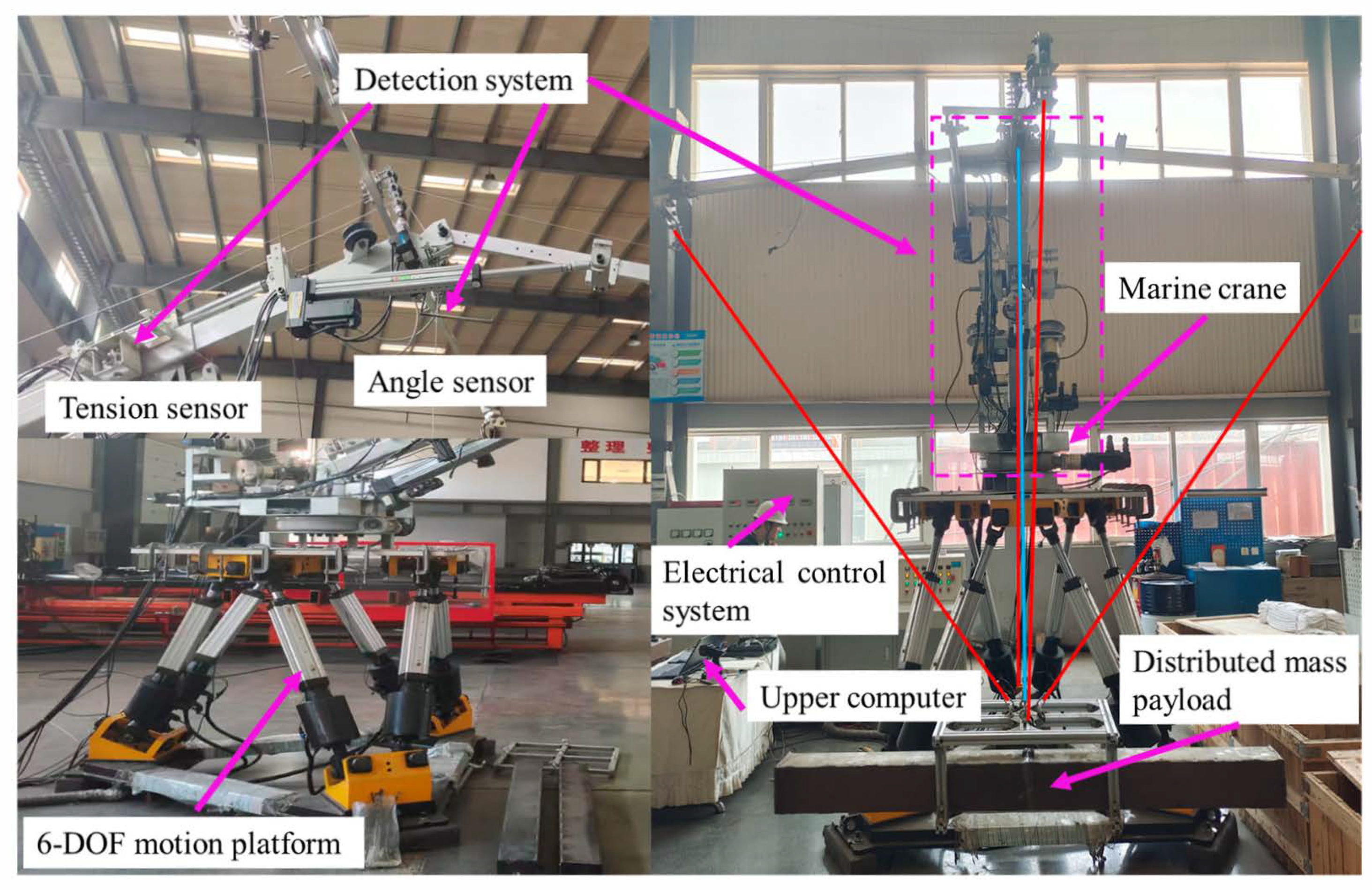
4. Experimental Study

The scaled-down experimental platform for the parallel anti-swing system of marine cranes is shown in Figure 11. It primarily consists of a six-degree-of-freedom motion platform, a scaled-down crane prototype, flexible cables (such as high-strength steel wire cables), driving devices (such as electric reels for controlling cable extension and retraction), a detection system (including tension sensors and angle sensors for monitoring system status), an electrical control cabinet, a control system, and a special spreader. The anti-swing system works as follows: anti-swing arms are installed at the front, rear, left, and right positions of the main boom, and the anti-swing cables are connected to the spreader/payload from four spatial directions via pulleys. Under the motion excitation of the ship’s six-degree-of-freedom motion platform, the upper computer receives tension signals from the anti-swing cables and swing signals from the payload. It then sends out command signals, which control the retracting and releasing actions of the anti-swing cables, ultimately suppressing the swing of the in-plane and out-of-plane angles of the DMP.

To investigate the swing suppression effect of the flexible cable parallel anti-swing system on DMP, the anti-swing control experiments of DMP with regular geometric shape and mass distribution and DMP with uneven irregular shape and mass distribution are conducted using the experimental platform shown in Figure 11. The marine environment is set to level 4 sea conditions; the ship motion excitation parameters in environment I are roll 4°, T = 13 s, pitch 0.9°, and T = 8 s; and the ship motion excitation parameters in environment II are roll 6°, T = 13 s, pitch 3°, and T = 8 s. The main boom length of the crane in the flexible cable parallel anti-swing system experimental platform is 2.45 m, and the main sling length is 1.6 m. The DMP with regular geometric shape and mass distribution has a length of 1.6 m and a mass of 32.6 kg. The DMP with irregular geometric shape and mass distribution is 1.6 m long and 4.6 kg. The tension sensors are LASCAUX models TR-100 kg and TR-200 kg, with accuracies of ±0.3 kg and ±0.6 kg, respectively. The angle sensor model is TE583C11M12P2B5F, with an accuracy of ±0.01°. Control system hardware: The controller of the electrical system is an AM403-CPU1608TN medium-sized PLC.

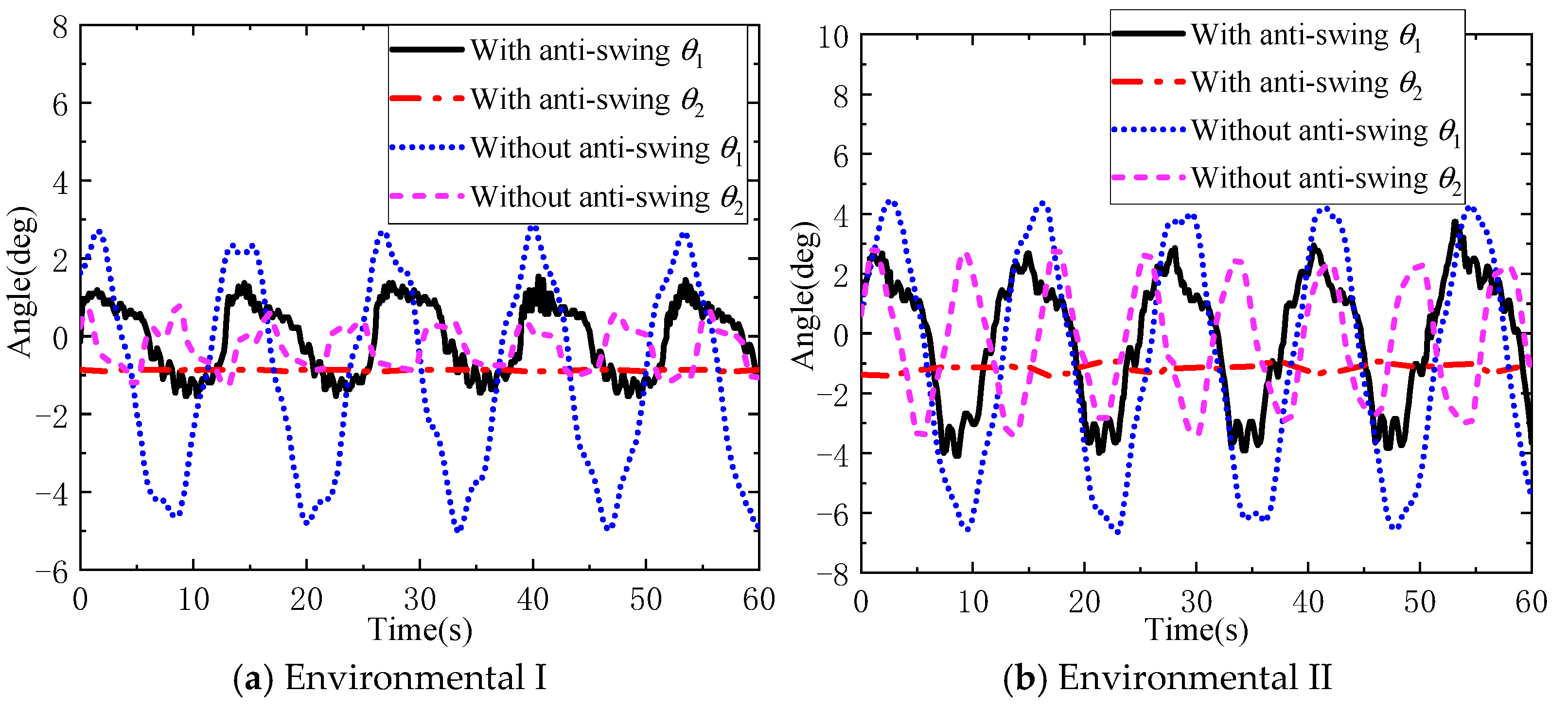
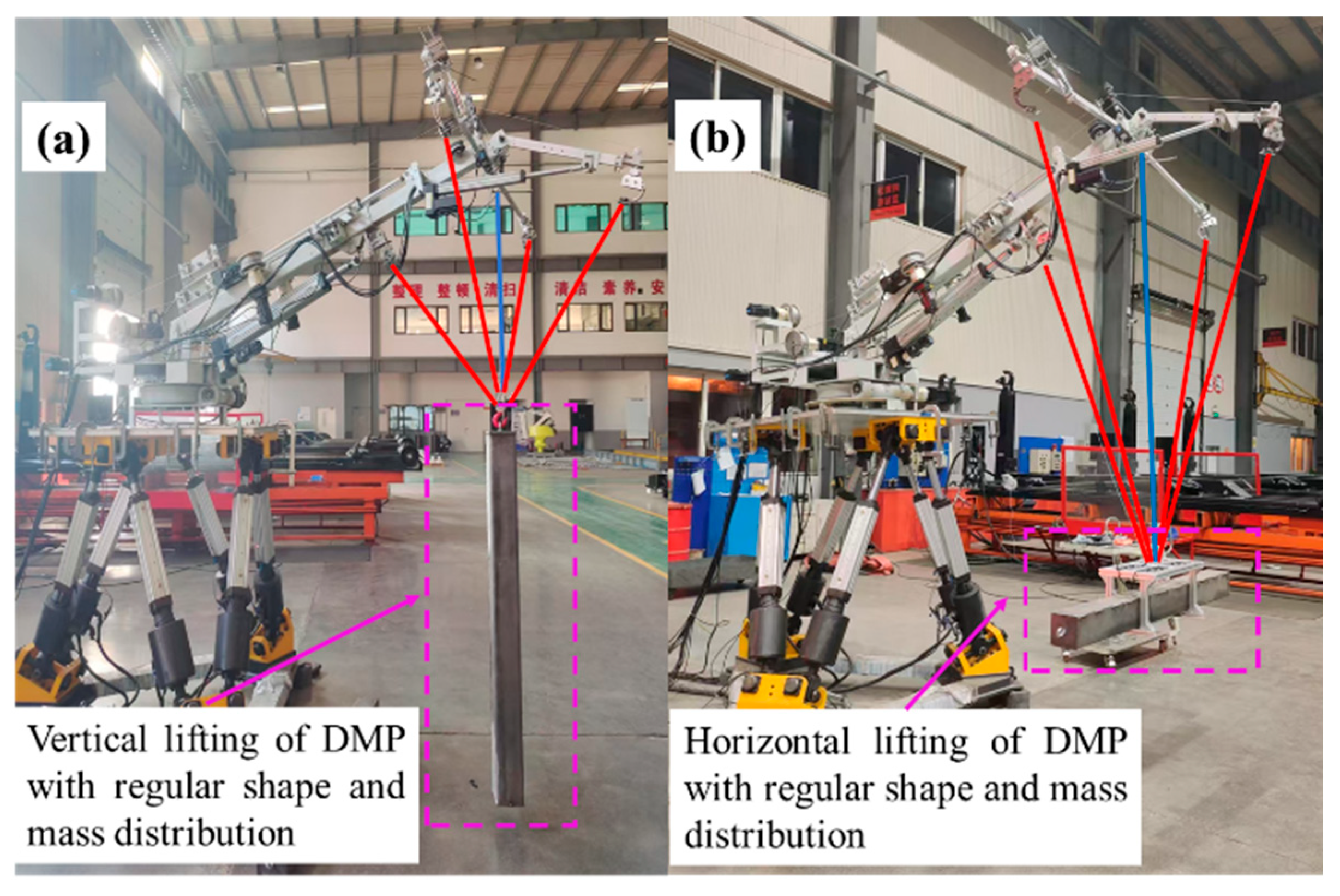
4.1. DMP Anti-Swing Experiment with Regular Shape and Mass Distribution

The experimental procedures for horizontal lifting of the DMP with regular shape and mass distribution are shown in Figure 11. The out-of-plane and in-plane angle anti-swing experiments are carried out in environments I and II, respectively.

It can be seen from Figure 12a that, in environment I without anti-swing control, the maximum in-plane and out-of-plane angles of the DMP are −5.05° and −1.22°, respectively, while with anti-swing control, the maximum in-plane and out-of-plane angles are 1.54° and −0.90°, respectively. The flexible cable parallel anti-swing system has an anti-swing effect of 69.5% and 25.8% on the in-plane and out-of-plane angles of the DMP with regular geometric shape and mass distribution, respectively. It can be seen from Figure 12b that, in environment II without anti-swing control, the maximum in-plane and out-of-plane angles of the DMP are −6.64° and −3.41°, respectively, and when there is anti-swing control, the maximum in-plane and out-of-plane angles are −4.09° and −1.41°, respectively. Furthermore, the flexible cable parallel anti-swing system has an anti-swing effect of 38.4% and 58.6% on the in-plane and out-of-plane angles of the DMP with regular geometric shape and mass distribution, respectively. In summary, the flexible cable parallel anti-swing system has a good swing suppression effect on the DMP with regular shape and mass distribution.

Next, anti-swing experiments are carried out on DMP with regular shapes and mass distributions under different lifting methods. The experimental process is shown in Figure 13a,b, and the results of the DMP anti-swing under the conditions of environment I are shown in Figure 14.

From Figure 14, it can be seen that, when using the flexible cable parallel anti-swing system for lifting DMP with regular shape and mass distribution, the maximum values of the in-plane and out-of-plane angles of the payload during vertical lifting are −3.517° and −0.571°, respectively. The maximum values of the in-plane and out-of-plane angles of the payload during horizontal lifting are −1.847° and −0.862°, respectively, with the in-plane angle decreasing by 47.5% and the out-of-plane angle increasing by 50.9% to 0.862°; the change is not more than 1°. Based on the above results, horizontal lifting has a better effect on reducing swing; therefore, for large DMP, horizontal lifting is generally selected, which can not only lower the centre of gravity, but also improve the anti-swing control effect to ensure the safety of lifting operations.

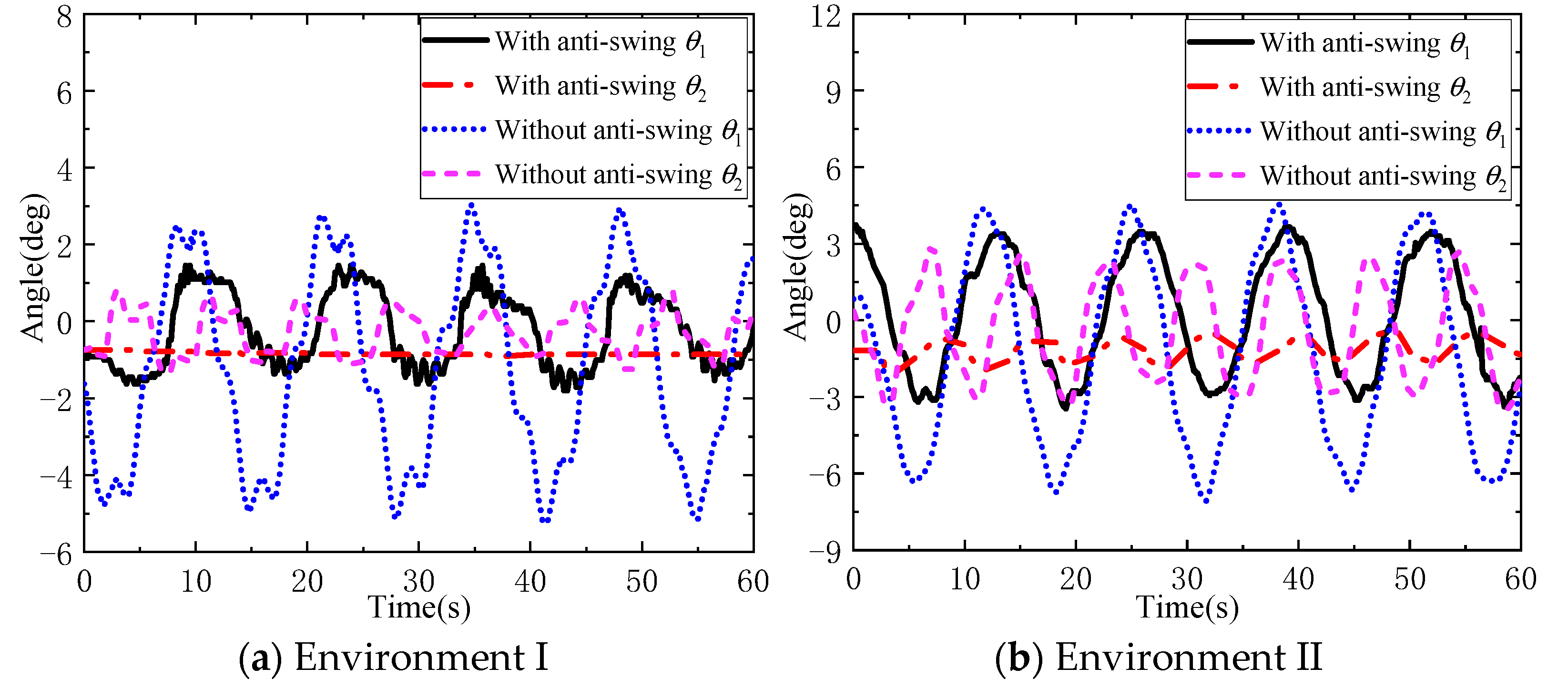
4.2. DMP Anti-Swing Experiment with Irregular Shape and Mass Distribution

It can be seen from Figure 15a that, in environment I without anti-swing control, the maximum in-plane and out-of-plane angles of the DMP with irregular shape and mass distribution are −5.23° and −1.29°, respectively, while with anti-swing control, the maximum in-plane and out-of-plane angles are 2.24° and −1.21°, respectively. The flexible cable parallel anti-swing system has an anti-swing effect of 57.1% and 6% on the in-plane and out-of-plane angles of the DMP with irregular geometric shape and mass distribution, respectively. From Figure 15b, it can be seen that, in environment II without anti-swing control, the maximum in-plane and out-of-plane angles of the DMP with irregular shape and mass distribution are −7.07° and 3.29°, respectively, and when there is anti-swing control, the maximum in-plane and out-of-plane angles are 3.64° and −1.99°, respectively. Furthermore, the flexible cable parallel anti-swing system has an anti-swing effect of 48.4% and 39.3% on the in-plane and out-of-plane angles of the DMP with irregular geometric shape and mass distribution, respectively. In summary, the flexible cable parallel anti-swing system still has a good swing suppression effect on the DMP with irregular shape and mass distribution.

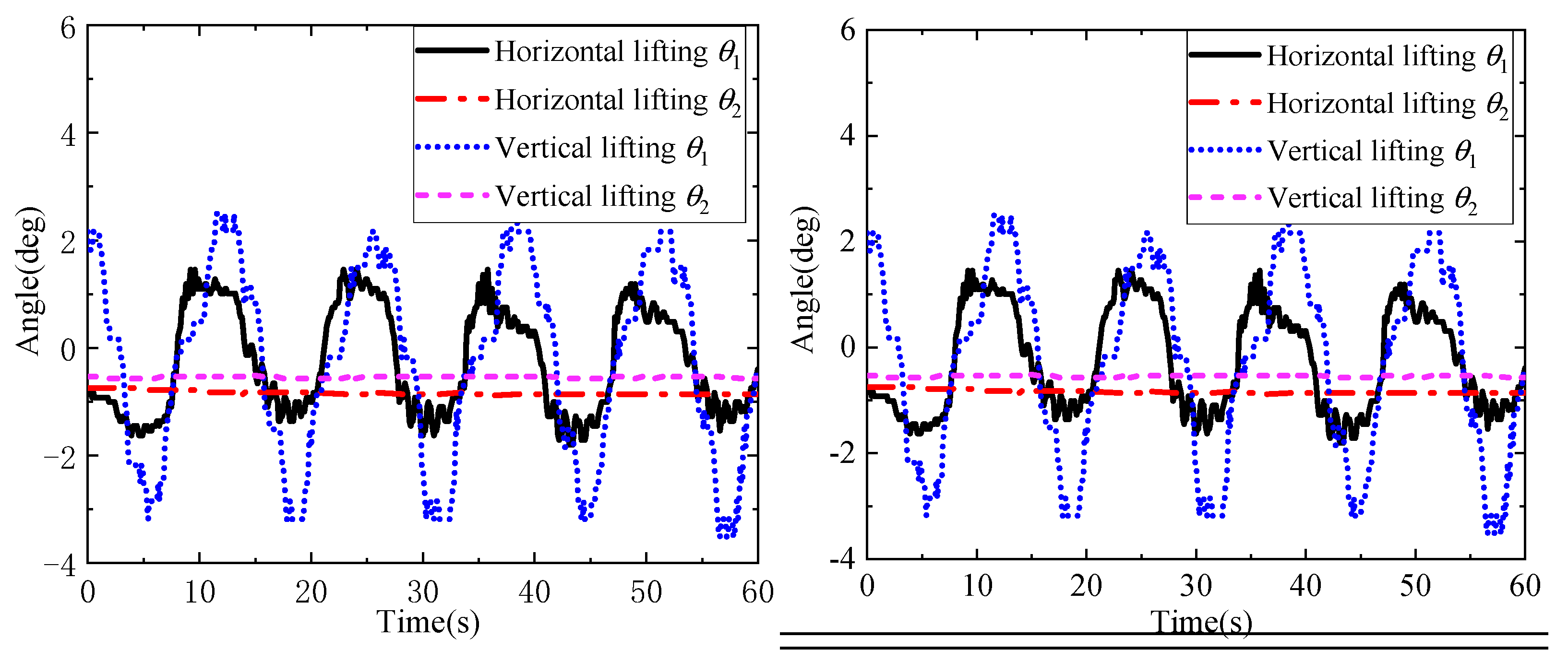
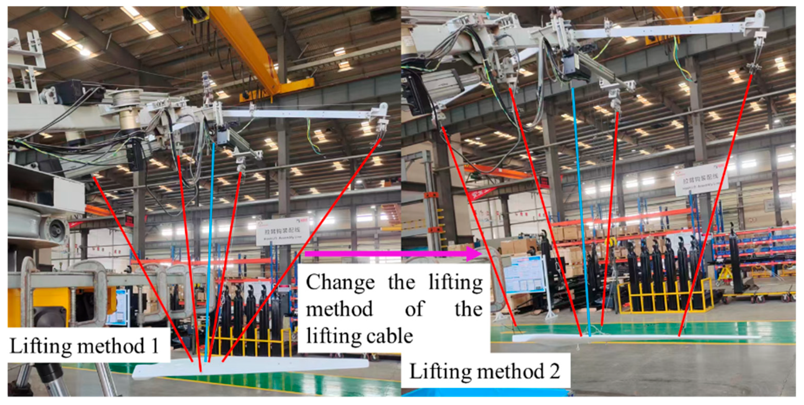
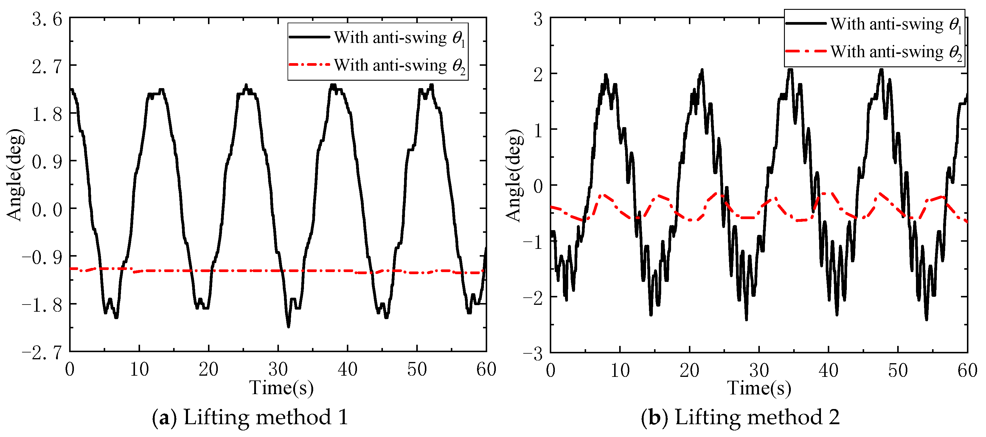
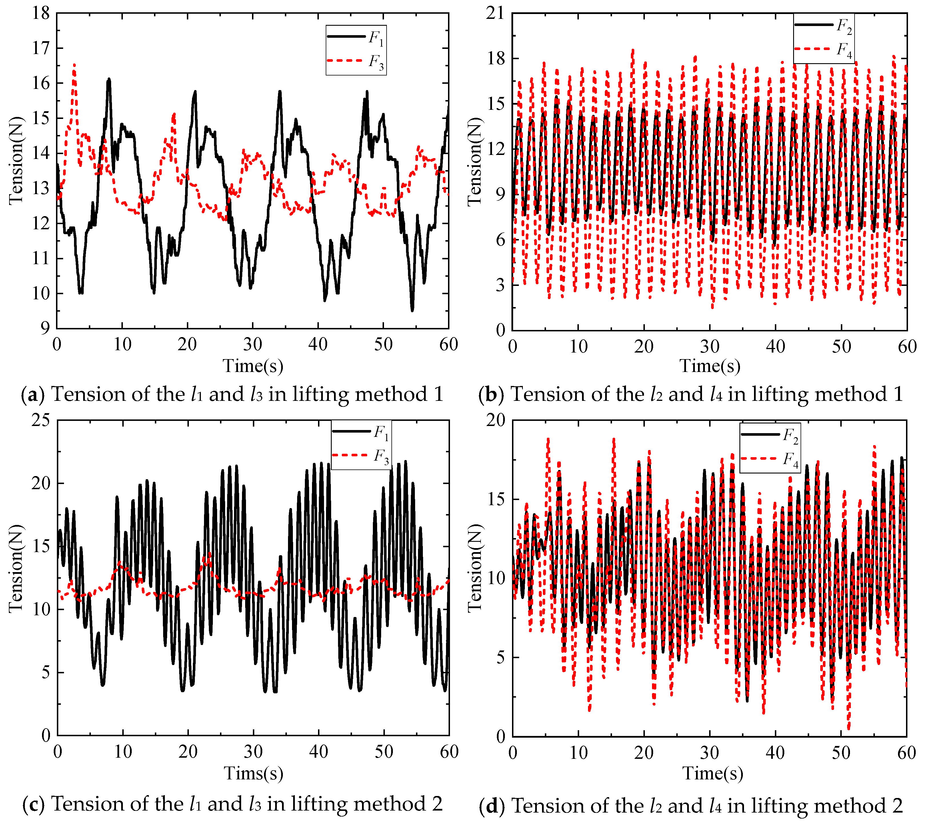
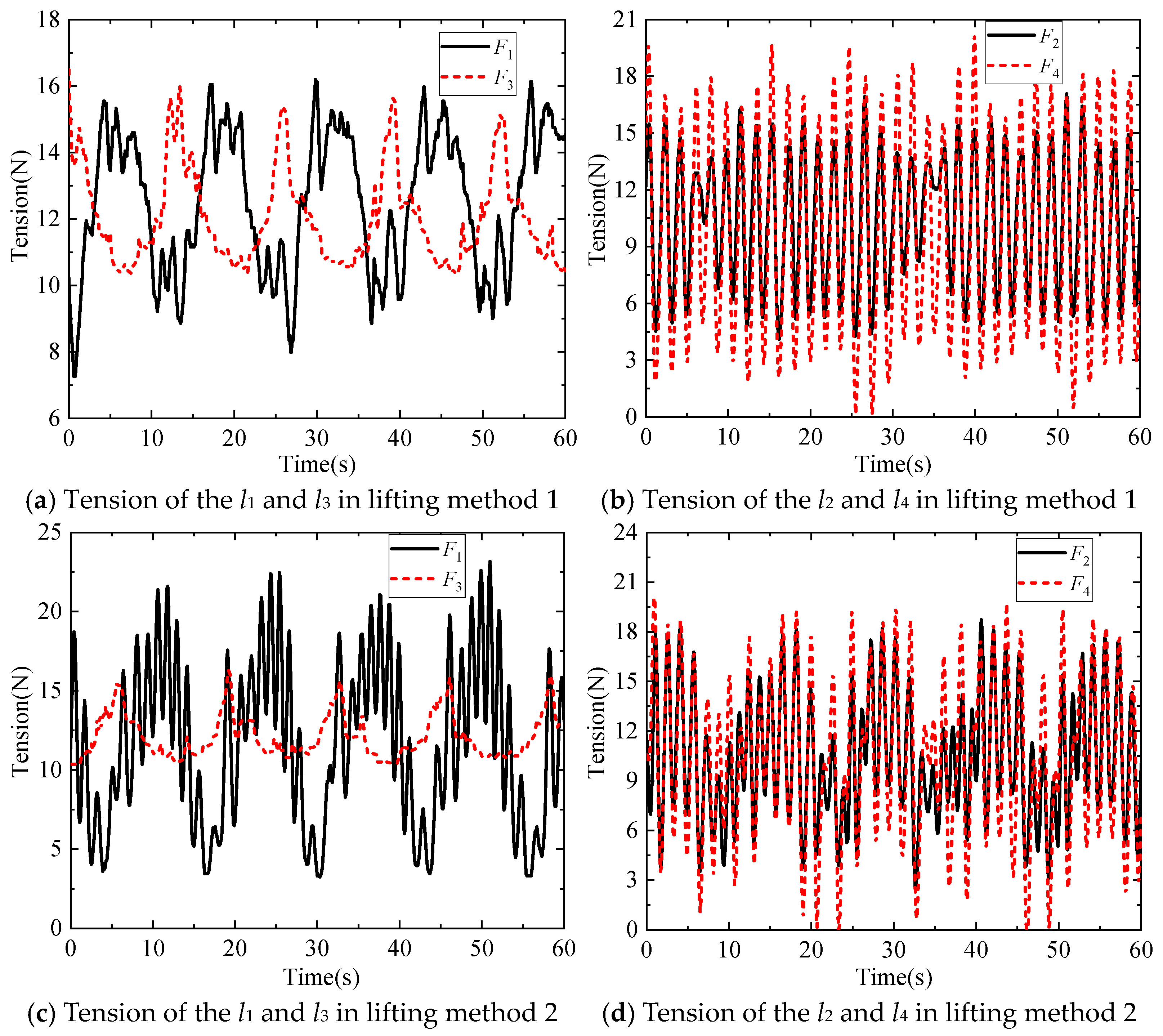
4.3. Irregularly Shaped DMP Anti-Swing Experiment Under Different Lifting Methods

To investigate the influence of different lifting methods on the DMP anti-swing, the DMP anti-swing experiment under different lifting methods is designed as shown in Figure 16.

In the experiments, the positions of the lifting points at the connection between the anti-swing cables l₁ and l₃ and the hook are changed to analyse whether changing the lifting distance in the horizontal direction of the DMP geometry could improve the anti-swing effect. The experimental results are shown in Figure 17, Figure 18, Figure 19 and Figure 20.

It can be seen from Figure 17 that, in lifting method 1, the maximum in-plane angle of the DMP is 2.33°, and the maximum out-of-plane angle is 1.25°, while in lifting method 2, the maximum in-plane angle of the DMP is 2.42°, and the maximum out-of-plane angle is 0.67°. From Figure 18 and Figure 20, it can be seen that the frequency of changes in the tensions of the anti-swing cables l₁, l₂, l₃, and l₄ is higher in lifting method 2 than in lifting method 1. Due to the influence of the mass distribution and geometric structure of the DMP, F₁ becomes larger, F₃ becomes smaller, the tensions F₂ and F₄ show a tendency to become larger, and the fluctuation of the magnitude of the tension force increases in lifting method 2.

Figure 19 shows that, in lifting method 1, the maximum in-plane angle of the DMP is 3.91° and the maximum out-of-plane angle is 3.02°. Compared with lifting method 1, the maximum in-plane angle of the payload in lifting method 2 is 3.82°, with little change, while the maximum out-of-plane angle is 1.45°, which is a decrease of 52.0%. Meanwhile, it can be seen from Figure 15 that the use of lifting method 2 helps to suppress the out-of-plane angle swing of the DMP with irregular shape and mass distribution.

5. Conclusions

The kinematic and static equations for the flexible cable parallel anti-swing system of the marine crane lifting a DMP are derived for various offshore engineering scenarios. Additionally, a dynamic coupling model is established for the ship, flexible cable parallel anti-swing system, and the DMP.

Under the maximum environmental excitation set in the experiment, the flexible cable parallel anti-swing system achieves swing suppression rates of 41.0% and 58.0% for the in-plane and out-of-plane angles of the DMP with regular geometric shape and mass distribution, respectively. For the DMP with irregular geometry and mass distribution, the suppression rates are 48.4% and 39.3% for the in-plane and out-of-plane angles, respectively. It is found that, after adjusting the lifting method and increasing the distance between lifting points, the maximum in-plane angle of the payload decreases by 2.3%, while the out-of-plane angle maximum decreases by 52.0%. These results demonstrate the effectiveness of adjusting lifting methods in suppressing swing for irregular DMPs, thereby verifying the reliability and applicability of the flexible cable parallel anti-swing system and providing a reference for improving anti-swing performance and lifting efficiency in offshore DMP operations.

References

1. Ren, Z.; Verma, A.S.; Ataei, B.; Halse, K.H.; Hildre, H.P. Model-free anti-swing control of complex-shaped payload with offshore floating cranes and a large number of lift wires. Ocean Eng. 2021, 228, 108868. [Google Scholar] [CrossRef]
2. Huang, J.; Liang, Z.; Zang, Q. Dynamics and swing control of double-pendulum bridge cranes with distributed-mass beams. Mech. Syst. Signal Pr. 2015, 54, 357–366. [Google Scholar] [CrossRef]
3. Tang, R.; Huang, J. Control of bridge cranes with distributed-mass payloads under windy conditions. Mech. Syst. Signal Pr. 2016, 72, 409–419. [Google Scholar] [CrossRef]
4. Sun, Z.; Ouyang, H. Adaptive fuzzy tracking control for vibration suppression of tower crane with distributed payload mass. Automat. Constr. 2022, 142, 104521. [Google Scholar] [CrossRef]
5. Yang, L.; Ouyang, H. Precision-positioning adaptive controller for swing elimination in three-dimensional overhead cranes with distributed mass beams. ISA T. 2022, 127, 449–460. [Google Scholar] [CrossRef]
6. Wu, Q.; Wang, X.; Hua, L.; Xia, M. Dynamic analysis and time optimal anti-swing control of double pendulum bridge crane with distributed mass beams. Mech. Syst. Signal Pr. 2020, 144, 106968. [Google Scholar] [CrossRef]
7. Miao, X.; Yang, L.; Ouyang, H. Artificial-neural-network-based optimal Smoother design for oscillation suppression control of underactuated overhead cranes with distributed mass beams. Mech. Syst. Signal Pr. 2023, 200, 110497. [Google Scholar] [CrossRef]
8. Wang, T.; Tan, N.; Zhang, X.; Li, G.; Su, S.; Zhou, J.; Scotti, F. A time-varying sliding mode control method for distributed-mass double pendulum bridge crane with variable parameters. IEEE Access 2021, 9, 75981–75992. [Google Scholar] [CrossRef]
9. Wu, Q.; Sun, N.; Wang, X. Equivalent rope length-based trajectory planning for double pendulum bridge cranes with distributed mass payloads. Actuators 2022, 11, 25. [Google Scholar] [CrossRef]
10. Wu, Q.; Sun, N.; Yang, T.; Fang, Y. Deep reinforcement learning-based control for asynchronous motor-actuated triple pendulum crane systems with distributed mass payloads. IEEE T. Ind. Electron. 2023, 71, 1853–1862. [Google Scholar] [CrossRef]
11. Albus, J.S.; Bostelman, R.V.; Dagalakis, N. The NIST robocrane. J. Res. Natl. Inst. of Stan. 1992, 97, 373–385. [Google Scholar] [CrossRef] [PubMed]
12. Gorman, J.J.; Jablokow, K.W.; Cannon, D.J. The cable array robot: Theory and experiment. In Proceedings of the 2001 ICRA. IEEE International Conference on Robotics and Automation (Cat. No. 01CH37164), Seoul, Republic of Korea, 21–26 May 2001; pp. 2804–2810. [Google Scholar]
13. Hiller, M.; Fang, S.; Mielczarek, S.; Verhoeven, R.; Franitza, D. Design, analysis and realization of tendon-based parallel manipulators. Mech. Mach. Theory 2005, 40, 429–445. [Google Scholar] [CrossRef]
14. Bosscher, P.; Williams II, R.L.; Bryson, L.S.; Castro-Lacouture, D. Cable-suspended robotic contour crafting system. Automat. Constr. 2007, 17, 45–55. [Google Scholar] [CrossRef]
15. Lamaury, J.; Gouttefarde, M.; Chemori, A.; Hervé, P.E. Dual-space adaptive control of redundantly actuated cable-driven. In Proceedings of the 2013 IEEE/RSJ International Conference on Intelligent Robots and Systems, Tokyo, Japan, 3–7 November 2013; pp. 4879–4886. [Google Scholar]
16. Korayem, M.H.; Bamdad, M.; Tourajizadeh, H.; Korayem, A.H.; Zehtab, R.M.; Shafiee, H.; Arvani, A. Experimental results for the flexible joint cable-suspended manipulator of ICaSbot. Robotica 2013, 31, 887–904. [Google Scholar] [CrossRef]
17. Revolutionary Crane Technology Is in Navy’s Future. Available online: https://www.nre.navy.mil/media-center/news (accessed on 2 May 2025).
18. Jung, Y.; Jang, I.G.; Kwak, B.M.; Kim, Y.K.; Kim, Y.; Kim, S.; Kim, E.H. Advanced sensing system of crane spreader motion (for mobile harbor). In Proceedings of the 2012 IEEE International Systems Conference SysCon 2012, Vancouver, BC, Canada, 19–22 March 2012; pp. 1–5. [Google Scholar]
19. Kim, Y.K.; Kim, Y.; Jung, Y.S.; Jang, I.G.; Kim, K.S.; Kim, S.; Kwak, B.M. Developing accurate long-distance 6-DOF motion detection with one-dimensional laser sensors: Three-beam detection system. IEEE T. Ind. Electron. 2012, 60, 3386–3395. [Google Scholar]
20. Kim, E.H.; Jung, Y.S.; Yu, Y.; Kwon, S.; Ju, H.; Kim, S.; Kim, K.S. An advanced cargo handling system operating at sea. Int. J. Control Autom. 2014, 12, 852–860. [Google Scholar] [CrossRef]
21. Hu, Y.; Tao, L.; Lv, W. Anti-pendulation analysis of parallel wave compensation systems. Proc. Inst. Mech. Eng. Part M J. Eng. Marit. Environ. 2016, 230, 177–186. [Google Scholar] [CrossRef]
22. Wang, J.; Wang, S.; Chen, H.; Niu, A.; Jin, G. Dynamic modeling and analysis of the telescopic sleeve antiswing device for shipboard cranes. Math. Probl. Eng. 2021, 2021, 6685816. [Google Scholar] [CrossRef]
23. Zhao, T.; Sun, M.; Wang, S.; Han, G.; Wang, H.; Chen, H.; Sun, Y. Dynamic analysis and robust control of ship-mounted crane with multi-cable anti-swing system. Ocean Eng. 2024, 291, 116376. [Google Scholar] [CrossRef]
24. Jin, G.; Wang, S.; Wang, J.; Wang, B.; Sun, Y.; Chen, H. Research on double pendulum anti-swing of cable-driven multi-point collaborative lifting for shipboard boom crane based on tension optimization. Proc. Inst. Mech. Eng. Part M J. Eng. Marit. Environ. 2025, 14750902251323653. [Google Scholar] [CrossRef]
25. Wu, Q.; Ouyang, H.; Xi, H. Adaptive nonlinear control for 4-DOF ship-mounted rotary cranes. Int. J. Robust Nonlin. 2023, 33, 1957–1972. [Google Scholar] [CrossRef]
26. Cao, M.; Xu, M.; Gao, Y.; Wang, T.; Deng, A.; Liu, Z. Advanced Control for Shipboard Cranes with Asymmetric Output Constraints. J. Mar. Sci. Eng. 2025, 13, 91. [Google Scholar] [CrossRef]
27. Mohd Tumari, M.Z.; Ahmad, M.A.; Suid, M.H.; Ghazali, M.R.; Tokhi, M.O. An improved marine predators algorithm tuned data-driven multiple-node hormone regulation neuroendocrine-PID controller for multi-input–multi-output gantry crane system. J. Low Freq. Noise V. A. 2023, 42, 1666–1698. [Google Scholar] [CrossRef]
28. Zhu, B.; Li, E.; Zhao, T.; Wang, C.; Tang, Z.; Li, Z. Dynamic characteristics of series-parallel hybrid rigid-flexible coupling double-mass underactuated system on floating platform. Mech. Mach. Theory 2023, 179, 105132. [Google Scholar] [CrossRef]
29. Leimeister, M.; Balaam, T.; Causon, P.; Cevasco, D.; Richmond, M.; Kolios, A.; Brennan, F. Human-free offshore lifting solutions. J. Phys. Conf. Ser. 2018, 1102, 012030. [Google Scholar] [CrossRef]
30. Jiang, Z. Installation of offshore wind turbines: A technical review. Renew. Sust. Energ. Rev. 2021, 139, 110576. [Google Scholar] [CrossRef]
31. Ren, Z.; Huang, Z.; Zhao, T.; Wang, S.; Chen, H.; Sun, Y.; Fang, N. Research on dynamic modeling and control strategy of four anti-swing cable system for ship-mounted cranes. Proc. Inst. Mech. Eng. Part M J. Eng. Marit. Environ. 2025, 239, 399–417. [Google Scholar] [CrossRef]
32. Youssef, K.; Otis, M.J.D. Reconfigurable fully constrained cable driven parallel mechanism for avoiding interference between cables. Mech. Mach. Theory 2020, 148, 103781. [Google Scholar] [CrossRef]
33. An, H.; Yuan, H.; Tang, K.; Xu, W.; Wang, X. A novel cable-driven parallel robot with movable anchor points capable for obstacle environments. IEEE/ASME T. Mech. 2022, 27, 5472–5483. [Google Scholar] [CrossRef]
34. Woziwodzki, S. Application of morison equation in unsteady mixing characteristics. In Practical Aspects of Chemical Engineering: Selected Contributions from PAIC 2019; Springer International Publishing: Cham, Switzerland, 2020; ISBN 9783030398675. [Google Scholar]
35. Miloh, T. Hamilton’s principle, Lagrange’s method, and ship motion theory. J. Ship Res. 1984, 28, 229–237. [Google Scholar] [CrossRef]
36. Cao, T.; Zhang, X. Nonlinear decoration control based on perturbation of ship longitudinal motion model. Appl. Ocean Res. 2023, 130, 103412. [Google Scholar] [CrossRef]
Figure 1. Cable parallel anti-swing system for a marine crane.
Jmse 13 01112 g001
Figure 2. Under-constrained model of the cable parallel anti-swing system for marine cranes.
Jmse 13 01112 g002
Figure 3. Catenary model of anti-swing cable.
Jmse 13 01112 g003
Figure 4. Schematic outline of the natural suspension of the anti-swing cables under different tensile forces.
Jmse 13 01112 g004
Figure 5. Schematic diagram of ship roll and pitch.
Jmse 13 01112 g005
Figure 6. Changes in wave inclination angle under different wave direction angles.
Jmse 13 01112 g006
Figure 7. Roll and pitch angle changes under different wave direction angles.
Jmse 13 01112 g007
Figure 8. Schematic diagram of the DMP lifting process.
Jmse 13 01112 g008
Figure 9. Schematic diagram of the static analysis of offshore wind turbine blades.
Jmse 13 01112 g009
Figure 10. Schematic diagram of ship–crane–DMP offshore lifting operations.
Jmse 13 01112 g010
Figure 11. Experimental platform for flexible cable parallel anti-swing system.
Jmse 13 01112 g011
Figure 12. Comparison experiment of DMP anti-swing with regular shape and mass distribution.
Jmse 13 01112 g012
Figure 13. DMP with regular shape and mass distribution under different lifting methods. (a) Vertical lifting, (b) Horizontal lifting.
Jmse 13 01112 g013
Figure 14. Comparison of anti-swing effects of DMP with regular shape and mass distribution under different lifting methods.
Jmse 13 01112 g014
Figure 15. Comparative experiment on DMP anti-swing with irregular shape and mass distribution.
Jmse 13 01112 g015
Figure 16. Experiments on the anti-swing of a DMP with different lifting methods.
Jmse 13 01112 g016
Figure 17. Influence of different lifting methods on the swing angle of a DMP in environment I.
Jmse 13 01112 g017
Figure 18. Influence of different lifting methods on the tension of anti-swing ropes in environment I.
Jmse 13 01112 g018
Figure 19. Influence of different lifting methods on the swing angle of a DMP in environment II.
Jmse 13 01112 g019
Figure 20. Influence of different lifting methods on the tension of anti-swing ropes in environment II.
Jmse 13 01112 g020