Joint Optimization of Multi-Period Empty Container Repositioning and Inventory Control Based on Adaptive Particle Swarm Algorithm

Abstract

This paper proposes a combined optimization method for multi-period empty container repositioning and inventory control based on adaptive particle swarm optimization (APSO) algorithm, which addresses the limitations of existing research, such as decoupling empty container repositioning and inventory control optimization, and lacking multi-period dynamic collaboration mechanisms. Firstly, a joint optimization model integrating (s, S) inventory control strategy is constructed. By adopting the strategy, the selection of repositioning paths and inventory resource allocation are synergistically optimized to balance unit empty container rental costs, inventory costs, and repositioning costs. Secondly, we design an adaptive particle swarm optimization algorithm, introduce dynamic inertia weight and acceleration coefficient adjustment mechanisms, and design heuristic rules for empty container repositioning. In this way, we reduce unreasonable empty container mobilization through the setting of surplus, shortage, and balance ports of empty containers, which can narrow the search space and improve the algorithm’s global search ability and convergence efficiency in high-dimensional decision spaces. Numerical experiments show that the joint optimization model designed can reduce the total cost of empty container management for shipping companies and maintain the rental cost in a stable state. Sensitivity analysis reveals that the unit container rental cost and the maximum inventory capacity of the port have a significant impact on the total system cost, providing a new approach for shipping companies to reduce empty container management costs.

1. Introduction

Against the backdrop of intensified global trade fluctuations, empty container repositioning, as a key link in the international logistics system, directly affects the resource utilization and cost control level of the maritime industry in terms of operational efficiency. Although empty container repositioning cannot directly bring profits to shipping companies, effective empty container repositioning can not only balance the supply and demand balance between shipping companies and container renting companies but also help reduce the cost of empty container inventory and the flow cost of empty containers between different regions. According to the International Chamber of Shipping, the global cost of empty container repositioning accounts for 20%~30% of the total operating cost of sea freight. In China, the cost of empty container repositioning accounts for more than 20% of the operating cost of container carriers. Empty container repositioning is a dynamic multi-period process, and the selection of transportation routes and ports directly affects the cost of empty container repositioning. At the same time, the quantity of empty container repositioning also directly affects the cost of empty container inventory at the port. Due to the time required for empty container replenishment, it is of great significance for shipping companies to use inventory control methods to reasonably arrange empty container repositioning in order to reduce total costs during operation. Therefore, in the process of empty container repositioning, scientifically and reasonably planning the empty container transportation path and inventory can effectively reduce the operating costs of shipping companies and improve the utilization rate of containers.

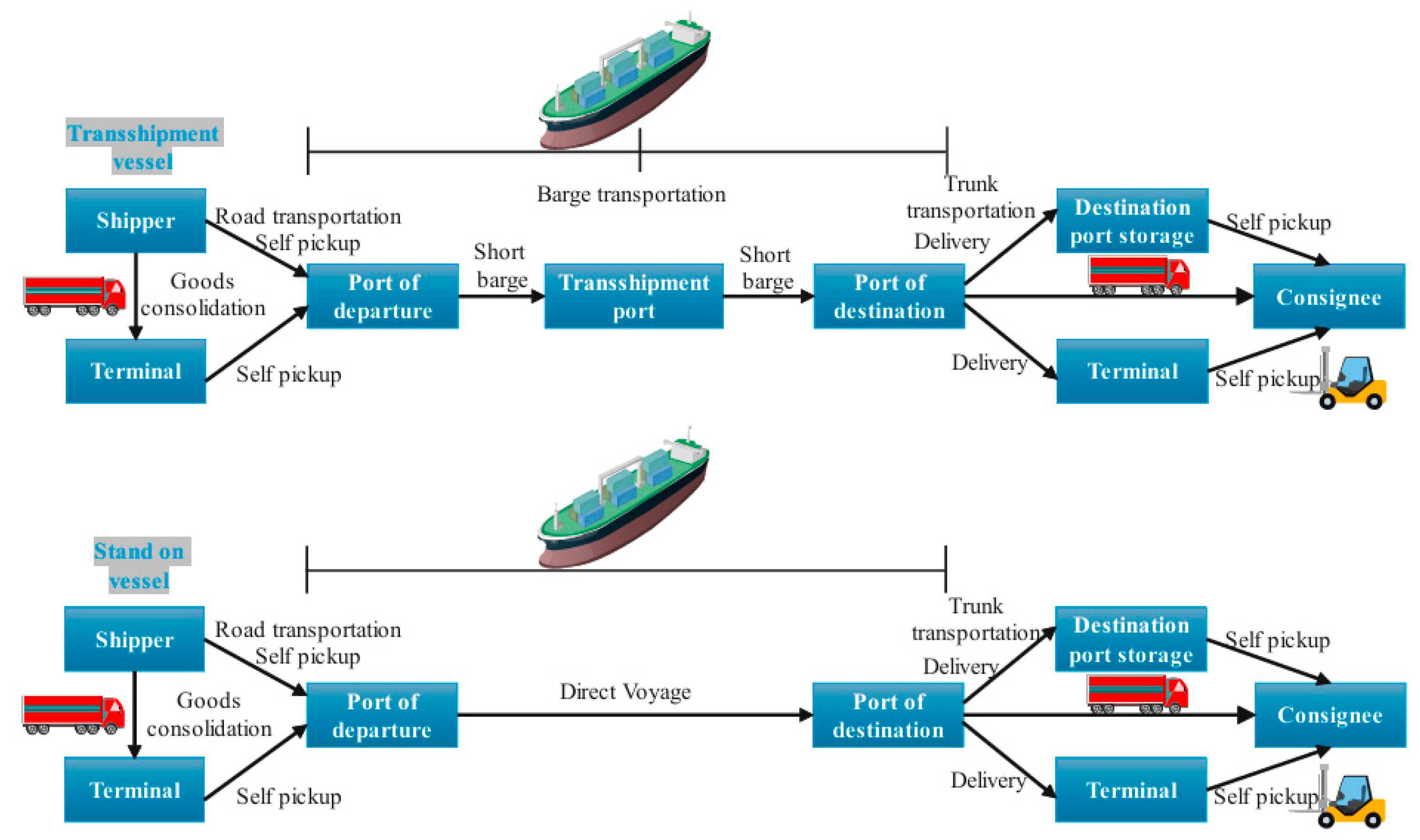
The complexity of empty container repositioning stems from its multi-party (shipping companies, ports, freight forwarders), multi-level (supplier networks, regional hubs), and multi-objective (cost minimization, carbon emission constraints) characteristics. Empty containers arise from the turnover process of containers. The turnover of containers must go through the process of unpacking and packing, which usually occurs at different times and locations. As shown in Figure 1, regardless of transshipment or direct shipping, the goods are shipped from inland areas. Inland shippers can transport the goods to terminals for consolidation or directly transport them by road to the port of departure. In order to meet the demand for empty containers for shipping goods, nearby ports, yards, and transit stations transport empty containers to the location of the shipper. If there is a shortage of empty containers at these locations, they need to be repositioned from other locations or rented from rental points outside the system. When the shipper’s demand for empty containers is met, the empty containers are loaded into the goods and become full containers, which are transported by sea to the destination port, where they may be stored in the destination port yard for the consignee to pick up, or transported to an inland terminal for the consignee to pick up. After unloading the goods, the full container becomes an empty container, which will be transported to nearby ports, yards, and terminals or returned to the container rental point. From the perspective of the circulation process, there are two aspects to consider when managing empty container resources: one is the allocation of empty container resources, and the other is inventory management of empty container resources.

In recent years, emergencies such as the Corona Virus Disease 2019(COVID-19) and geopolitical conflicts have occurred frequently, leading to problems such as port congestion and imbalance of transport capacity. The traditional static inventory management model makes it difficult to cope with dynamic demand fluctuations. Although existing research has made some progress in the field of empty container repositioning optimization (such as path planning and inventory target optimization), there are still significant gaps in the collaborative optimization of inventory control and repositioning from a multi-period perspective. Most studies decouple inventory strategies (such as reorder points and safety inventory) from transportation scheduling, ignoring the interactive effects of the two in multi-period dynamic scenarios. Due to the different source structures and flow of goods in each region, it is easy to lead to an extreme shortage of containers in a certain port, an imbalance of inventory caused by the accumulation of empty containers in a certain port, and the risk of insufficient supply of empty containers and excess empty container resources in the empty container supply chain system at any time. In addition, in the design of empty container repositioning algorithms, most designs revolve around precise algorithms or traditional heuristic algorithms and do not reflect the characteristics of empty container repositioning and inventory problems in the algorithm design process. This is also one of the drawbacks of the research on empty container repositioning. Therefore, this paper proposes a joint optimization problem of multi-period empty container repositioning and storage under the $\left(s,S\right)$ inventory control strategy, where s represents the ordering point, and S represents the maximum inventory level, providing a scientific and effective strategy for the management of empty container resources in shipping companies. By designing an APSO algorithm with heuristic rules that have the characteristics of empty container repositioning problems, the specificity of the algorithm can be increased.

The remainder of this paper is organized as follows. Section 2 provides a review of previous research on empty container repositioning and inventory and presents the relevant contributions of this paper. Section 3 provides a detailed analysis of the problem to be studied in this paper. Section 4 proceeds with the construction of the mathematical model. Section 5 elaborates on the implementation process of the APSO algorithm. Subsequently, numerical experiments were conducted based on the designed algorithm in Section 6. Finally, in Section 7, the conclusion of this paper and the next steps of work are presented.

2. Literature Review

This paper conducts a literature review from three aspects: first, optimization of empty container repositioning over multiple periods; second, inventory control strategies for empty containers; and finally, joint optimization of empty container repositioning and inventory control over multiple periods.

2.1. Research on Optimization of Empty Container Repositioning Under Multi-Period

The optimization of empty container repositioning has shifted from the initial single period to multi-period. The research on multi-period empty container repositioning optimization is more in line with the characteristics of empty container repositioning problems. The iteration of empty container repositioning volume between different periods also helps to reduce unnecessary circulation of empty container resources and overall management costs.

From the perspective of research on empty container repositioning strategy, Xu et al. [1] studied the problem of empty container repositioning in maritime logistics and proposed an integrated adaptive reinforcement learning framework to adjust the weights of multi-objective reward functions. Cai et al. [2] applied machine learning algorithms to predict the supply and demand of empty containers, and two different optimization models for empty container repositioning strategies were proposed to minimize the total kilometers of empty container turnover. Tao and Wu [3] introduced the concept of a “yard-port” transportation chain and semi-life cycle assessment, considering the energy consumption and carbon dioxide emissions during loading and unloading and empty container repositioning. Francesco et al. [4] believed that the uncertainty of port emergencies would have a serious impact on empty container repositioning and simulated the actual situation of empty container repositioning when emergencies occur. Lin and Juan [5] proposed a solution framework that considered empty container sharing and exchange strategies, including a platform company for empty container matching and a shipping company for a given route, to coordinate the empty container allocation problem through the design of two-layer programming.

From the perspective of vessel scheduling and network design, Xiang et al. [6] explored the comprehensive optimization problem of empty container repositioning and ship scheduling and developed a new branch-price algorithm to illustrate the impact of container turnover time on empty container repositioning. Numa-Navarro et al. [7] explored the issue of empty container repositioning within the Colombian region, reduced the accumulation of a large number of empty containers in the repositioning network, and proved that the street turn mode was an effective strategy to improve the efficiency of empty container repositioning. Tang et al. [8] constructed a multi-period empty container repositioning optimization model with the lowest total cost and stable network by combining the container-sharing strategy. The Lyapunov optimization method was used to effectively achieve container repositioning and sharing. Yoonjea et al. [9] explored the optimization problem of a bidirectional four-layer multimodal transport network for direct shipping between two ports, including a land transportation subsystem. Lu et al. [10] constructed a stochastic dynamic programming model to study the joint decision-making of shipping pricing and empty container allocation with stochastic empty container demand in a dual warehouse shipping system. Furio et al. [11] established two mathematical models based on the street-turn model to optimize container repositioning between inland shippers, consignees, and port terminals, minimizing inventory costs in the transportation system.

Although these models have considered the characteristics of multi-period empty container repositioning problems and incorporated factors such as multiple ports and routes, they have also overlooked the important issue of the constantly changing inventory of empty containers by shipping companies. Compared to existing models, this paper focuses more on the judgment of surplus and shortage of containers to determine the direction of empty container repositioning.

2.2. Research on Empty Container Inventory Control Strategy

The decision regarding empty container inventory can be divided into two directions. One is to combine the problem of empty container inventory with empty container repositioning, optimize the inventory of empty containers through repositioning, or make decisions on empty container repositioning based on the empty container inventory control. Liang et al. [12] studied a new dynamic allocation strategy that determines the repositioning decision of empty containers for each period based on the current empty container inventory, completed demand, and average demand in future periods. Mehrzadegan et al. [13] integrated dynamic cargo allocation, empty container repositioning, and inventory management decisions in liner shipping, utilizing multi-segment revenue management to maximize the profits of shipping companies within a limited decision period. Rajeswari et al. [14] studied the impact of container misplacement on reusable empty container inventory management and used an empty container “first in–first out” strategy to reduce inventory costs. Luo and Chang [15] studied the inventory management problem of empty containers when customer demand changes in multimodal transport systems and discussed the impact of empty container repositioning on the optimal inventory level. Poo and Yip [16] dynamically controlled the inventory and repositioning costs of empty containers in feeder transportation in a dynamic environment to reduce the imbalance between full and empty containers.

The second is to use mathematical methods, such as fuzzy mathematics, stochastic programming, etc., to construct inventory models and obtain optimal decisions related to empty container inventory. Sarmadi et al. [17] constructed a two-stage stochastic programming model that combined dynamic inventory decision-making in uncertain environments with the number and location of dry ports, providing guidance for container network configuration and inventory turnover in the shipping industry. Grag et al. [18] took container management agencies as the research subject and studied a container inventory model considering delayed returns and price-sensitive demand in the fuzzy domain. Grag et al. [19] constructed a container inventory model using the expected value of trapezoidal numbers to avoid the shortage of reusable empty containers, ultimately minimizing system costs. Legros et al. [20] managed empty containers through a threshold strategy to save on the cost of using empty containers. Guo et al. [21] studied the inventory and scheduling decision-making problem on a shared platform for reusable transportation items (including containers, pallets, etc.) and designed a machine learning and simulation optimization decision framework to solve the inventory and scheduling decisions of the two-layer container management center.

The empty container inventory threshold calculation in existing models is often static, and more attention is paid to the impact of empty container repositioning decisions on empty container inventory, such as Luo and Chang [15]. This paper focuses on how the empty container inventory threshold affects empty container repositioning decisions in a constantly fluctuating state.

2.3. Research on Joint Optimization of Empty Container Repositioning and Inventory Control

From the perspective of the type of joint optimization model constructed, Yang et al. [22], by constructing a two-stage game model, studied the impact of information warfare on container transportation problems to achieve cost minimization. Kamal [23] designed a causal mechanism model under the background of empty container repositioning, considering the impact of seasonal fluctuations and trade volume fluctuations on shipping company decisions. Wang et al. [24] designed an optimization model for empty container repositioning using queuing theory and minimized the total cost of empty container repositioning and inventory. Zhou et al. [25] designed a separable and segmented linear learning algorithm to solve its two-stage stochastic programming model. Rajeswari et al. [26] used the theory of fuzzy inventory to construct a fuzzy empty container inventory model to optimize the optimal length of empty container repositioning and leasing period. Abdelshafie et al. [27] constructed a modeling framework for empty container repositioning, forming an agent-based modeling paradigm that reduces the total cost for shipping companies in empty container management.

From the joint optimization perspective, Najafi and Zolfagharinia [28] optimized the problem of empty container repositioning to maximize profits for shipping companies, combined with price management theory. In non-stationary demand environments, Lee and Moon [29] constructed a model for empty container repositioning considering foldable containers and proposed a robust formula for empty container repositioning as a paradigm for subsequent optimization of empty container repositioning. Chi et al. [30] have optimized the quantity and inventory of empty containers repositioned from surplus areas to shortage areas by considering three modes of transportation: sea, road, and railway. Siswanto et al. [31], under the constraints of multiple transportation time windows, solved the problem of empty container repositioning, and comprehensive optimization of ship path optimization and container loading and unloading volume was achieved. Castrellon et al. [32] studied two empty container repositioning strategies—one is the street-turn mode, and the other is the strategy of extending free storage time—and evaluated the advantages and disadvantages of these two empty container repositioning strategies.

2.4. Research Gap

Based on the existing literature research mentioned above, the following areas for further optimization can be summarized.

(1)

Decision decoupling problem

Most existing studies have separated inventory strategy from transportation scheduling, neglecting the dynamic impact of setting empty container inventory thresholds on multi-period repositioning path selection. At the same time, optimizing the empty container inventory threshold can also synchronously reduce the empty container repositioning and rental volume. The inventory, rental, and repositioning volume are interrelated, but static inventory thresholds cannot meet the needs of periodic changes in repositioning and rental volume. Therefore, establishing dynamic inventory thresholds is necessary for optimizing empty container repositioning.

(2)

Model adaptability limitations

Most inventory control strategies perform well in single-node, single-period scenarios, but the spatiotemporal correlation and nonlinear cost characteristics in multi-port networks make it difficult to expand directly. How to extend the classic inventory control strategy model to multi-period and multi-port empty container repositioning scenarios is also a key issue that needs further optimization.

2.5. Major Contributions

Based on the practical needs of the industry and the insufficient research in existing literature, the main contributions of this paper are as follows:

(1)

By constructing a joint optimization model for empty container repositioning and empty container inventory, the dynamic inventory empty container threshold is used to control the empty container repositioning volume, breaking the original optimization mode of optimizing empty container inventory through empty container repositioning volume. The threshold decision of inventory replenishment point (s) and maximum inventory level (S) is integrated with repositioning path selection and capacity allocation to reveal the dynamic trade-off mechanism between inventory cost and repositioning cost.

(2)

Under the application of the (s, S) empty container inventory control strategy, empty container repositioning rules are designed under the threshold setting of empty container inventory, as well as status judgment rules for surplus and shortage containers. These heuristic rules are added to the APSO algorithm, making the overall algorithm design more prominent in the prominent characteristics of empty container repositioning problems and providing a new algorithm design approach for solving the joint optimization problem of empty container repositioning and empty container inventory.

3. Problem Formulation

This paper assumes that shipping company A provides transportation services in a certain area with different ships of the same type. The inventory of empty containers at different ports is a constantly changing process for the shipping company. During its daily operation, the supply and demand of empty containers vary with the change in full container volume. When the vessel arrives at the port, the unloaded full containers become an empty container supply, while the full containers that need to be loaded onto the vessel for shipment are the demands for empty containers at the port.

Due to the imbalance of trade, there are three types of empty container ports: surplus, shortage, and balance ports. After meeting the demand for empty containers in the port, the surplus port will reposition the remaining empty container to the shortage port for use. The shortage port needs to meet the demand for empty containers through container repositioning and renting, while the shortage port does not reposition containers externally. Balance ports mean neither repositioning in nor out. For the surplus ports of shipping companies, the decision to reposition excess empty containers to other ports is based on the maximum value of empty container inventory, which is the upper limit. When the inventory of empty containers exceeds the maximum value, the unloading of empty containers will no longer be carried out when the ship docks at the surplus port. For shortage ports, a safety inventory level, i.e., a lower limit, is required. When the empty container inventory level is lower than the safety level, it is necessary to reposition containers from other ports or rent containers locally to meet the demand for empty containers in the port while no longer repositioning empty containers externally.

This paper starts from the perspective of shipping companies and optimizes the empty container repositioning routes and ship docking ports to obtain the optimal quantity of empty container repositioning, as well as the safety and maximum inventory levels of empty containers at different ports. Ultimately, the goal is to minimize the sum of empty container repositioning costs, inventory costs, and rental costs for shipping companies under multi-periods. The optimization of empty container repositioning paths and effective inventory control are combined.

4. Mathematical Model

4.1. Assumptions

To better address this issue, this paper proposes the following assumptions:

(1)

Vessels are different ships of the same type from the same shipping company;

(2)

Without considering the purchase of new containers, the shipping company can rent containers without considering the return of rented containers;

(3)

Without considering the load capacity, measure according to the load capacity of each TEU standard;

(4)

Without considering transshipment transportation, containers will not proceed to the next round of transportation after being unloaded at a certain port;

(5)

Each vessel on each route must dock at least one port;

(6)

All empty container demands must be met, and no shortage of containers is allowed.

4.2. Notation Description

(1)

Set

Notation descriptions of the sets are shown in

Table 1. Notation description of sets.

Notation	Description
$T$	Decision period, $t\in T$.
$S$	Set of departure port, $s\in S$.
$D$	Set of unloading port, $d\in D$, and $S\cap D=\varnothing$.
$P$	Set of port, $p\in P$.
$V$	Set of vessels from one shipping company, $v\in V$.
$A$	Set of all arcs, $a\in A$.
$N$	Set of all nodes, $n\in N$. For each node, it is a pair of port-period—i.e., $n=(p,t),p\in P,t\in T$.

.

(2)

Parameters

Notation descriptions of parameters are shown in

Table 2. Notation description of parameters.

Notation	Description
$C{A}_v^{\max }$	The maximum container load of a container vessel.
$C{I}_d$	Unit empty container inventory cost at the unloading port $d\in D$.
$I{V}_p^0$	Initial empty container inventory at the port $p\in P$.
${\lambda }_a^v$	Unit empty container repositioning cost when vessel $v\in V$ sailing at arc $a\in A$.
$CR$	Unit rental cost.
$I{V}_d^{\max }$	The maximum inventory capacity of the port $d\in D$.
$q{1}_{dt}^v$	The quantity of full containers unloaded by the vessel $v\in V$ at the unloading port $d\in D$ in the period $t\in T$, converted into empty container supply.
$q{2}_{dt}^v$	The number of full containers transported by the vessel $v\in V$ at the unloading port $d\in D$ in the period $t\in T$, which is the demand for empty containers.

.

(3)

Decision variables

Notation descriptions of decision variables are shown in

Table 3. Notation description of decision variables.

Notation	Description
$Q_{pdt}^v$	The quantity of empty container repositioning of the vessel $v\in V$ from the port $p\in P$ to the unloading port $d\in D$ in the period $t\in T$.
$x_{at}^v$	(0,1) decision variable. If the stage vessel $v\in V$ is sailing on the arc $a\in A$ in the period $t\in T$, the value is 1; otherwise, it is 0.
$I{V}_{dt}$	Available empty container inventory of the unloading port $d\in D$ at the beginning of $t\in T$.
$L_{dt}$	The rental quantity of empty containers at the port $p\in P$ in the period $t\in T$.
$z_{dt}$	(0,1) decision variable, whether container renting occurs at the unloading port$d\in D$ in the period $t\in T$.

.

(4)

Derivative variables

Notation descriptions of derivative variables are shown in

Table 4. Notation description of derivative variables.

Notation	Description
${\omega }_{pt}$	The difference between empty container inflows and outflows at the port $p\in P$ in the period $t\in T$.
$W_p^t$	The quantity of empty containers that need to be repositioned by the port $p\in P$ in the period $t\in T$. When $W_p^t<0$, it indicates that supply exceeds demand, and empty containers need to be repositioned outward. When $W_p^t\ge 0$, it indicates that supply is less than demand, and empty containers need to be repositioned inward.
$y_{pt}^v$	(0,1) variable. If the vessel $v\in V$ is loading and unloading cargo at the port $p\in P$ in the period $t\in T$, the value is 1; otherwise, it is 0.
$X{X}_p^t$	(0,1) variable, whether to reposition empty containers to the port $p\in P$ in the period $t\in T$.

.

4.3. Empty Container Repositioning Model

The objective function is to minimize the total empty container management cost of the shipping company, which includes three parts: empty container repositioning cost, empty container inventory cost, and empty container renting cost, as shown in Formula (1).

$$\min ={\displaystyle \sum _{t\in T}{\displaystyle \sum _{v\in V}{\displaystyle \sum _{a\in A}{\displaystyle \sum _{p\in P}{\displaystyle \sum _{d\in D}{Q}_{pdt}^v}}{\lambda }_a^v{x}_{at}^v+{\displaystyle \sum _{t\in T}{\displaystyle \sum _{d\in D}I{V}_{dt}C{I}_d+{\displaystyle \sum _{t\in T}{\displaystyle \sum _{d\in D}{z}_{dt}CR}}}}}}}{L}_{dt}$$

(1)

This is subjected to the following:

$${\displaystyle \sum _{a\in {\theta }^{+}(n)}{x}_{at}^v-{\displaystyle \sum _{a\in {\theta }^{-}(n)}{x}_{at}^v={\mu }_n}},\forall v\in V,\forall t\in T,\forall n\in N$$

(2)

$${\theta }^{+}(n)=\left\{\left(n,n^{\prime }\right)\in A\right\},{\theta }^{-}(n)=\left\{\left(n^{\prime },n\right)\in A\right\},\forall n\in N$$

(3)

$$W_p^t={\displaystyle \sum _{v\in V}{\displaystyle \sum _{a\in {\theta }^{-}(n)}{x}_{at}^v}q{2}_{dt}^v-I{V}_{dt},\forall d\in D,\forall t\in T},\forall p\in P$$

(4)

$$0\le Q_{pdt}^v+q{1}_{dt}^v-q{2}_{dt}^v\le y_{pt}^{v}C{A}_v^{\max },\forall v\in V,\forall d\in D,\forall t\in T,\forall p\in P$$

(5)

$$\begin{array}{c}I{V}_{dt}=I{V}_{d(t-1)}+{\displaystyle \sum _{v\in V}(q{1}_{dt}^v-q{2}_{dt}^v)}+{\displaystyle \sum _{v\in V}{\displaystyle \sum _{p\in P}[X{X}_p^t{Q}_{pdt}^v-\left(1-X{X}_p^t\right)Q_{dpt}^v]}}\le I{V}_d^{\max }\\ \forall d\in D,\forall t\in T,\forall p\in P\end{array}$$

(6)

$$I{V}_{d(t-1)}+y_{pt}^v(q{1}_{dt}^v+X{X}_p^t{Q}_{pdt}^v)+z_{dt}{L}_{dt}\ge y_{pt}^{v}q{2}_{dt}^v,\forall v\in V,\forall d,p\in D,\forall t\in T$$

(7)

$${\displaystyle \sum _{v\in V}{\displaystyle \sum _{p\in P}{Q}_{dpt}^v\le \left|W_p^t\right|}},\forall t\in T,\forall d\in D$$

(8)

$${\displaystyle \sum _{v\in V}{\displaystyle \sum _{p\in P}{Q}_{pdt}^v+z_{pt}{L}_{dt}\ge \left|W_p^t\right|,\forall t\in T,\forall d\in D}}$$

(9)

$${\displaystyle \sum _{v\in V}{\displaystyle \sum _{p\in P}X{X}_p^t{Q}_{pdt}^v+z_{dt}{L}_{dt}-{\displaystyle \sum _{v\in V}{\displaystyle \sum _{p\in P}(1-X{X}_p^t)Q_{pdt}^v\ge W_p^t,\forall t\in T}}}},\forall d\in D$$

(10)

$$0\le L_{dt}\le \left|W_p^t\right|,\forall d,p\in P,\forall t\in T$$

(11)

$${\displaystyle \sum _{p\in P}{y}_{pt}^v\ge 1,\forall v\in V,\forall t\in T}$$

(12)

$$y_{pt}^v\le {\displaystyle \sum _{a\in {\theta }^{-}(n)}{x}_{at}^v},\forall v\in V,\forall t\in T,\forall p\in P$$

(13)

$${\displaystyle \sum _{a\in A}{x}_{at}^v=1,\forall v\in V,\forall t\in T}$$

(14)

$$X{X}_p^t=\left\{\begin{array}{l}1,W_p^t\ge 0\\ 0,W_p^t<0\end{array}\right.,\forall t\in T,\forall p\in P$$

(15)

$$z_{pt}=\left\{\begin{array}{l}1,{\omega }_{pt}\ge 0\\ 0,{\omega }_{pt}<0\end{array}\right.,\forall t\in T,\forall p\in P$$

(16)

$$x_{at}^v\in (0,1),y_{at}^v\in (0,1),z_{pt}\in (0,1),\forall v\in V,\forall a\in A,\forall t\in T$$

(17)

$$Q_{pdt}^v,L_{dt},I{V}_{dt}\ge 0 , Q_{pdt}^v,L_{dt},I{V}_{dt}are \mathrm{integers},\forall t\in T,\forall d\in D,\forall v\in V,\forall p\in P$$

(18)

Constraints (2) and (3) represent the determination of the departure port (${\mu }_n=1$), intermediate port (${\mu }_n=0$) (the vessel does not load or unload at the port), and unloading port (${\mu }_n=-1$). Constraint (4) represents the quantity of empty containers that need to be repositioned by the port. Constraint (5) indicates that the loading and unloading capacity of full and empty containers cannot exceed the maximum container capacity of the vessel. Constraint (6) represents the inventory of empty containers in the port. Constraint (7) indicates that when a vessel docks at a port, the demand for empty containers must be met. Constraints (8)–(10) represent the balance of inflow and outflow of empty containers. Constraint (11) is a constraint on the rental quantity. Constraint (12) indicates that the vessel must call at least one port on each route. Constraint (13) indicates that there will be no loading or unloading operations without a port of call. Constraint (14) represents that each arc on a route can only be sailed once per period. Constraints (15)–(17) are constraints on the variable (0,1). Constraint (18) represents the non-negative integer constraint on the decision variable.

4.4. Empty Container Inventory Control Model

According to the characteristics of empty container repositioning and inventory control strategy, this paper adopts the $\left(s,S\right)$ inventory strategy to optimize and analyze the inventory issues involved in the process of empty container repositioning. The principle of this strategy is that when the storage strategy is greater than $s$, it will not be repositioned, and when it is less than $s$, it will be repositioned to replenish inventory and make the inventory reach its maximum value $S$. This value is the maximum inventory quantity that meets customer demand and minimizes inventory costs. In the problem of empty container repositioning, the value $s$ is equivalent to the safety inventory level of the container shortage port. When the inventory is lower than this level, the demand for empty containers can no longer be met. At this time, empty container repositioning or container renting must be carried out. The value $S$ is equivalent to the maximum inventory level of empty containers stored at the surplus container port. If the inventory exceeds this value, external container repositioning must be carried out. Excessive inventory of empty containers will bring additional inventory costs to the shipping company.

Assuming that the supply of empty containers does not allow for stockouts and the replenishment time for empty containers is zero [33]. The demand for empty containers, which is the full container transportation volume mentioned above, is represented $r$ here and follows a continuous density function $g_d^t\left(r\right),\forall t\in T,\forall d\in D$. Simultaneously, we introduce new (0,1) variables ${\alpha }_d^t,\forall t\in T,\forall d\in D$. When the port repositions containers, its value is 1; otherwise, it is 0. We introduce $S_d^t$ to indicate the holding quantity of empty containers at the port $d\in D$ in the period $t\in T$. Its value is the sum of the initial inventory level and empty container repositioning volume for each period: $S_d^t=I{V}_{dt}+{\displaystyle \sum _{v\in V}{\displaystyle \sum _{p\in P}{Q}_{pdt}^v}},\forall t\in T,\forall d\in D$. Therefore, we can obtain the following formula for the expected cost of all empty container inventories from multiple demand points to multiple supply points.

When $S_d^t\ge r$, the expected cost is as follows:

$$E\left[C_1\left(S_d^t\right)\right]={\displaystyle \sum _{a\in A}{\displaystyle \sum _{t\in T}{\displaystyle \sum _{d\in D}{\displaystyle \sum _{v\in V}\left[{\displaystyle {\int }_0^{S_d^t}{C}_d\left(S_d^t-r\right)CR\left(r-S_d^t\right)d{g}_d^t\left(r\right)+{\alpha }_d^t{\lambda }_a^v{x}_a^v\left(S_d^t-I{V}_{dt}\right)}\right]}}}}$$

(19)

When $S_d^t<r$, the expected cost is as follows:

$$E\left[C_2\left(S_d^t\right)\right]={\displaystyle \sum _{a\in A}{\displaystyle \sum _{t\in T}{\displaystyle \sum _{d\in D}{\displaystyle \sum _{v\in V}\left[{\displaystyle {\int }_{S_d^t+1}^{\infty }CR\left(r-S_d^t\right)d{g}_d^t\left(r\right)+{\alpha }_d^t{\lambda }_a^v{x}_a^v\left(S_d^t-I{V}_{dt}\right)}\right]}}}}$$

(20)

Therefore, we can obtain the total expected cost, which can be expressed as follows:

$$\begin{array}{c}E\left[C\left(S_d^t\right)\right]={\displaystyle \sum _{a\in A}{\displaystyle \sum _{t\in T}{\displaystyle \sum _{d\in D}{\displaystyle \sum _{v\in V}{\displaystyle {\int }_0^{S_d^t}{C}_d\left(S_d^t-r\right)CR\left(r-S_d^t\right)d{g}_d^t\left(r\right)}}}}}\\ +{\displaystyle {\int }_{S_d^t+1}^{\infty }CR\left(r-S_d^t\right)d{g}_d^t\left(r\right)+{\alpha }_d^t{\lambda }_a^v{x}_a^v\left(S_d^t-I{V}_{dt}\right)}\end{array}$$

(21)

By taking the derivative of $E\left[C\left(S_d^t\right)\right]$ and making it 0, we can obtain $S$, which is the maximum inventory of empty containers in the surplus container port.

To obtain the value of safety inventory $s$, we use the marginal analysis method. If the shipping company does not conduct empty container repositioning at the port $d\in D$ at the beginning of the period, the expected cost at this time is the following:

$$E\left[C_3\left(I{V}_{dt}\right)\right]={\displaystyle \sum _{t\in T}{\displaystyle \sum _{d\in D}{\displaystyle {\int }_0^{I{V}_{dt}}{C}_d\left(I{V}_{dt}-r\right)d{g}_d^t\left(r\right)+{\displaystyle {\int }_{I{V}_{dt}+1}^{\infty }CR\left(r-I{V}_{dt}\right)d{g}_d^t\left(r\right)}}}}$$

(22)

If the shipping company conducts empty container repositioning at the port $d\in D$ at the beginning of the period, the expected cost is as follows:

$$E\left[C_4\left(S_d^t\right)\right]={\displaystyle \sum _{v\in V}{\displaystyle \sum _{a\in A}{\displaystyle \sum _{t\in T}{\displaystyle \sum _{d\in D}{\displaystyle {\int }_0^{S_d^t}{C}_d\left(S_d^t-r\right)d{g}_d^t(r)}}}}}+{\displaystyle {\int }_{S_d^t+1}^{\infty }CR\left(r-S_d^t\right)d{g}_d^t}\left(r\right)+x_a^v{\lambda }_a^v\left(S_d^t-I{V}_{dt}\right)$$

(23)

From the above two formulas, if $E\left[C_3\left(I{V}_{dt}\right)\right]\ge E\left[C_4\left(S_d^t\right)\right]$, there is no need for empty container repositioning. In other words, the following can be established:

$$\begin{array}{c}{\displaystyle \sum _{t\in T}{\displaystyle \sum _{d\in D}\left[{\displaystyle {\int }_0^{I{V}_{dt}}{C}_d\left(I{V}_{dt}-r\right)d{g}_d^t\left(r\right)+{\displaystyle {\int }_{I{V}_{dt}+1}^{\infty }CR\left(r-I{V}_{dt}\right)d{g}_d^t\left(r\right)}}\right]}}\\ \ge {\displaystyle \sum _{v\in V}{\displaystyle \sum _{a\in A}{\displaystyle \sum _{t\in T}{\displaystyle \sum _{d\in D}\left[{\displaystyle {\int }_0^{S_d^t}{C}_d\left(S_d^t-r\right)d{g}_d^t(r)}+{\displaystyle {\int }_{S_d^t+1}^{\infty }CR\left(r-S_d^t\right)d{g}_d^t}\left(r\right)+x_a^v{\lambda }_a^v\left(S_d^t-I{V}_{dt}\right)\right]}}}}\end{array}$$

(24)

From this inequality, when $I{V}_{dt}=S_d^t,\forall d\in D,\forall t\in T$, the inequality is clearly valid, indicating that this inequality must have a solution. When $I{V}_{dt}<S_d^t$, the minimum value of $I{V}_{dt}$ that satisfies the inequality is the value of the safety inventory $s$ that is being calculated.

5. Design of APSO Algorithm Based on Heuristic Rules

5.1. Design Ideas

As we can see from the mathematical model constructed earlier, it is a nonlinear mixed integer programming model that cannot be solved using exact solvers such as CPLEX. Secondly, in the traditional heuristic algorithm-solving process, more attention is paid to the design of the implementation process of the algorithm itself, and the specificity of the solving problem is often overlooked. The problem to be studied in this paper is the dynamic and multi-periodic empty container repositioning problem under the coordination of inventory control strategies. During the repositioning process, it is necessary to pay constant attention to the surplus and shortage status of shipping companies at various ports and monitor the changes in empty container inventory under the constraints of inventory control strategies. These key contents need to be emphasized in the algorithm design process. Therefore, based on the APSO algorithm, this paper incorporates heuristic rules for determining the status of surplus and shortage, as well as inventory threshold restrictions, making the implementation process of the algorithm more in line with the characteristics of the problem while also reducing unnecessary search processes and improving algorithm efficiency. Especially in the numerical example setting of this paper, which includes multiple decision cycles, multiple ports, multiple vessels, and multiple routes, the scale of the example is relatively large. The design of heuristic rules also makes the algorithm solution more convenient and efficient. At the same time, it should be emphasized that in the research on optimizing decision-making for empty container repositioning problems, heuristic rules related to surplus container quantity, shortage container quantity, and empty container inventory threshold control have not yet been integrated into the adaptive particle swarm algorithm, which means that there are no previous results we can use for reference. Here, we only focus on demonstrating the implementation process and calculation results of the algorithm designed in this paper.

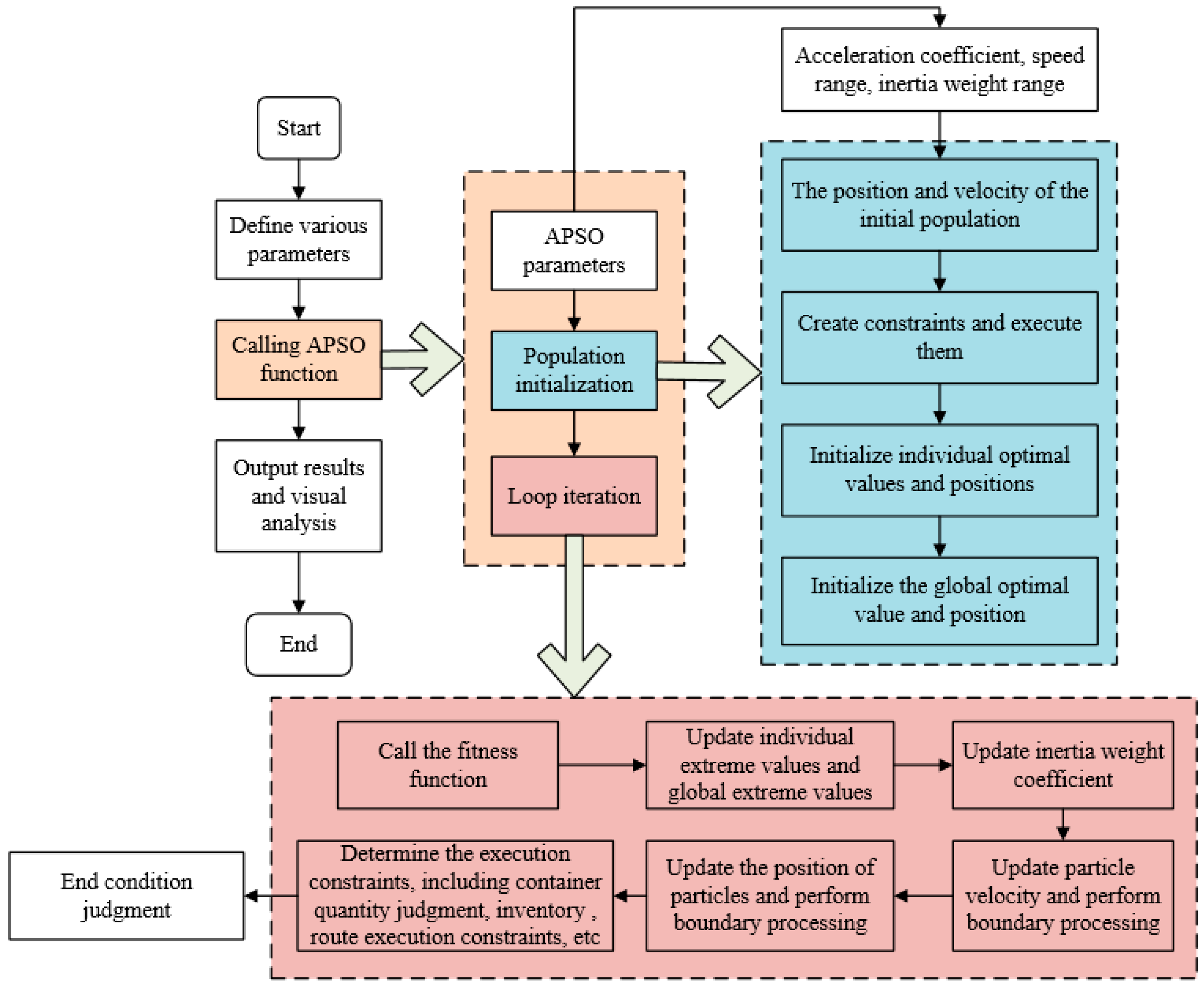
Additionally, the traditional particle swarm optimization (PSO) algorithm performs well in some problems but still faces challenges such as premature convergence, high parameter sensitivity, high-dimensional problems, and multimodal limitations. In order to enhance the algorithm’s ability to perform global search in the initial stage and local search and convergence in the later stage, this paper adopts adaptive strategies to improve the traditional particle swarm algorithm, making it more in line with the characteristics of optimizing empty container transportation problems. The algorithm flowchart is shown in Figure 2.

5.2. APSO Algorithm Parameter Settings

The weights of the standard PSO algorithm are fixed values, which makes the particle swarm algorithm prone to becoming stuck in local optima. Dynamic inertia weight can adaptively adjust the weight according to different stages of the search process, thereby better balancing global exploration and local optimization and improving the search ability of the algorithm. Therefore, we define $w$ as the inertia weight, which should be larger in the early stage and smaller in the later stage. The dynamic changes after improvement are shown in the calculation Formula (25).

$$w=w_{\max }-\left(w_{\max }-w_{\min }\right)*\left(iter-1\right)/\left(ite{r}_{\max }-1\right)$$

(25)

$w_{\max }$ is the initial value of inertia weight, $w_{\min }$ is the minimum value of inertia weight, and $iter$ is the number of iterations.

Secondly, the speed $v$ update formula is shown in Equation (26), the lower bound of the speed $v_{\min }$ is shown in Equation (27), and the maximum amplitude of the speed $v_{\max }$ is shown in Equation (28). This paper sets it as half of the variable range.

$$v=w*v+c_1*r_1*\left(pbest-current\right)+c_2*r_2(gbest-current)$$

(26)

$$v_{\min }=-v_{\max }$$

(27)

$$v_{\max }=\left(ub-lb\right)*0.5$$

(28)

$c_1$, $c_2$ are individual and social learning factors, respectively. $r_1$, $r_2$ are random numbers of (0,1). $pbest$, $gbest$ are optimal positions for local and global particles, respectively. $current$ is the current position. $ub$, $lb$ are the upper and lower limits of the empty container repositioning capacity.

The updated formula for particle position is shown in Equation (29).

$$x_i^{t+1}=x_i^t+v_i^{t+1}$$

(29)

$x_i^{t+1}$ indicates the position $i$ of particles in the period $t+1$, $x_i^t$ is the position $i$ of particles in the period $t$, and $v_i^{t+1}$ is the speed of position $i$ in the period $t+1$.

5.3. Heuristic Rules Design

To combine the path optimization in the empty container repositioning model with inventory control, relevant rules for determining the surplus container port, shortage container port, and balance port are designed in the algorithm, and transportation rules are set for different container quantity states. As shown in the following three rules.

• Set the formula for judging the status of empty container quantity: $D\left(p,t\right)=supply\left(p\right)-demand\left(p\right),\forall p\in P,\forall t\in T$. Based on $D\left(p,t\right)$, determine the type of each port in each cycle as follows: surplus port $\left(D>0\right)$, shortage port $\left(D<0\right)$, balanced port $\left(D=0\right)$.
• A shortage port is always in a state of container shortage, and the demand for empty containers cannot be met in a timely manner. Therefore, in a container shortage port, the issue of maximum inventory does not need to be considered, but the safety stock level should be taken into account. If the inventory of empty containers in the port is lower than the safety stock level, the demand of the container shortage port will not be met. At the same time, once the inventory level has dropped below the safety stock level—that is, $Q_{dpt}^v=0,\forall v\in V,\forall d,p\in P,\forall t\in T$—there will be no further external container transfers until the inventory level returns to being above the safety stock level.
• There are many empty containers stored in the surplus container port; hence, the issue of safety stock is not considered. Instead, the maximum inventory level is considered. When the empty container inventory is more than the maximum inventory level, it is necessary to continuously transfer containers outward and not accept empty container unloading from other ports, $Q_{pdt}^v=0,\forall v\in V,\forall d,p\in P,\forall t\in T$, until it is below the maximum inventory level before proceeding with empty container unloading.

In the design of this paper, we stipulate that empty containers are only allowed to flow from the surplus port to the shortage port and are not allowed to be empty or no empty repositioning in other cases. Therefore, we only set particle variables for the voyage segment with “departure port as surplus port and destination port as shortage port” to reduce search space.

5.4. Algorithm Process Design

The detailed process of Algorithm 1 is shown below.

Step1: Initialize the empty container repositioning and inventory control model and assign values to parameters such as unit inventory cost and unit rental cost.

Step2: Randomly initialize the position and velocity of the particle swarm, with the initial velocity set to a random value not exceeding $v_{\max }$. The random initialization must ensure that it is within the range of $\left[lb,ub\right]$. Each particle position is represented by a $1*nVar$ vector to represent the value of each transport variable, and the velocity is also a $1*nVar$ vector.

Step3: Evaluate the initial solution fitness and update the global optimal particle position.

Step4: Adaptively adjust the inertia weight according to Formula (25), update the velocity according to Formula (26), control the velocity boundary according to Formulas (27) and (28), update the particle position according to Formula (29), and then conduct position boundary control.

Step5: Evaluate the fitness values of all particles and compare them with the objective function (1). If the fitness value is greater than the average fitness value, it indicates that the particles are far away from the minimum value, and the search range needs to be expanded to find the maximum value. At this time, the position update change will be greater. If the fitness value is less than the average fitness value, it indicates that the particle is closer to the minimum distance. The algorithm needs to narrow down the search scope for local precise search, which needs to be achieved by speeding up. Then update $pbest$ and $gbest$.

Step6: Traverse each period and port, update inventory and container rental status, and fill in empty container repositioning decisions based on particle positions;

Step7: Perform an iterative search on the entire algorithm space until the maximum number of iterations is reached. Next, output the results, parse the global best position $gbest$ into repositioning decisions, and calculate various costs and indicators.

The pseudocode of Algorithm 1 is shown below.

Algorithm 1: APSO

for each particle $i$

Initialize velocity $v_i$ and position $x_i$ for particle $i$  Evaluate particle $i$ and set $pbest=x_i$

end for

$gbest=\min \left(pbest\right)$

while not stop

for i = 1 to N

Update the velocity and position of particle $i$   Evaluate particle $i$

if fit $\left(x_i\right)$ < fit $\left(pbest\right)$

$pbest=x_i$;

if fit $\left(pbest\right)$ < fit $\left(gbest\right)$

$gbest=pbest$;

end for

end while

print $gbest$

end procedure

6. Numerical Experiment

6.1. Parameter Setting

In the APSO algorithm, we set the number of population particles to 50; the number of iterations to 500; $w_{\max }$, $w_{\min }$ to 0.9 and 0.4, respectively; with both $c_1$, $c_2$ values being 2.0.

This paper sets up five ports, with a total of four ships executing four routes. Starting from one port and returning to that port is considered as one voyage, forming a closed loop. According to the frequency of shipping, a cycle of 7 days is set, and the decision period number is 4.

The container shipping market is influenced by many factors, and the situation is complex. Decisions often need to be constantly adjusted, and the decision-making period cannot be too long. In addition, the analysis of previous literature also indicates that it is not meaningful to extend the influence period of decision-making on the basis of a sufficiently long influence period. Therefore, based on reality, taking a month as the unit, dividing one month into four small planning periods, scheduling the repositioning plan once a week, that is, making decisions at the beginning of each month, while generating immediate costs, only affecting the empty container status and management for the next three weeks.

The unit rental fee is set at 500 yuan/TEU, and the unit empty container repositioning cost is set to be related to each arc, that is, each voyage, as shown in

Table 5. Unit empty container repositioning cost for each voyage segment.

Route/Voyage	Cost (yuan/TEU)	Route/Voyage	Cost (yuan/TEU)
1/1→2	20	3/5→1	35
1/2→3	30	3/1→2	42
1/3→1	25	3/2→5	30
2/3→4	40	4/2→5	52
2/4→5	50	4/5→4	23
2/5→3	45	4/4→2	25

. The other related cost settings of the port are shown in

Table 6. Port-related costs.

Port	Initial Inventory (TEU)	Unit Inventory Cost (yuan/TEU)	Max Inventory (TEU)
1	0	50	400
2	10	45	300
3	5	40	300
4	0	32	300
5	5	48	200

.

6.2. Calculation Results

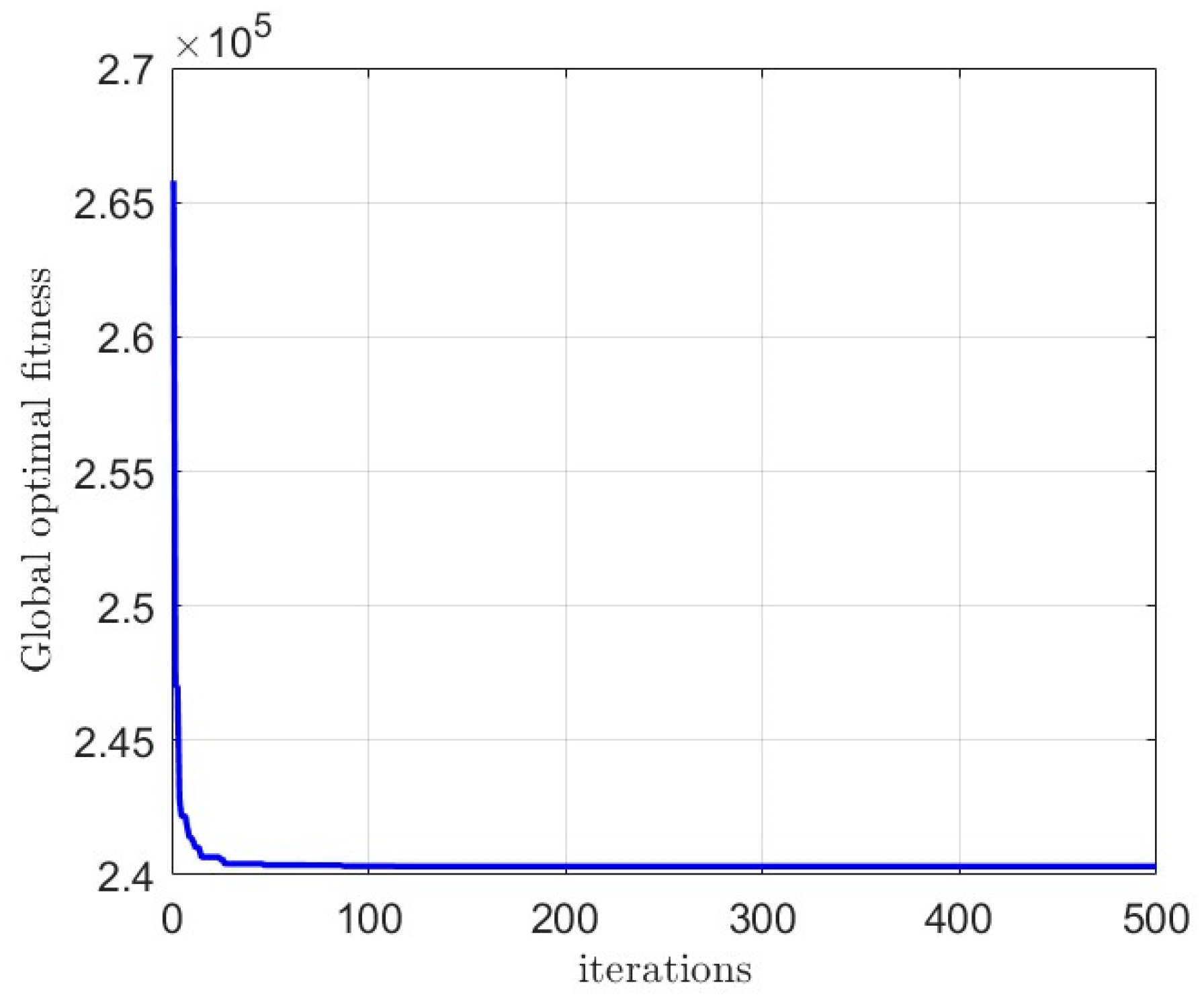
Using the APSO algorithm designed in this article, the model was solved, and the convergence curve of the APSO algorithm is shown in Figure 3. The calculation results are shown in Figure 4, and the optimal empty container transportation plan is shown in

Table 7. Optimal empty container repositioning scheme.

Period	Vessel	Repositioning Routes	Quantity of Empty Container Repositioning
	1	2→3	50
1	3	2→5	118
2	2	4→5	10
3	1	3→1	20
3	4	2→5	20
4	1	3→1	70
4	3	5→1	10

.

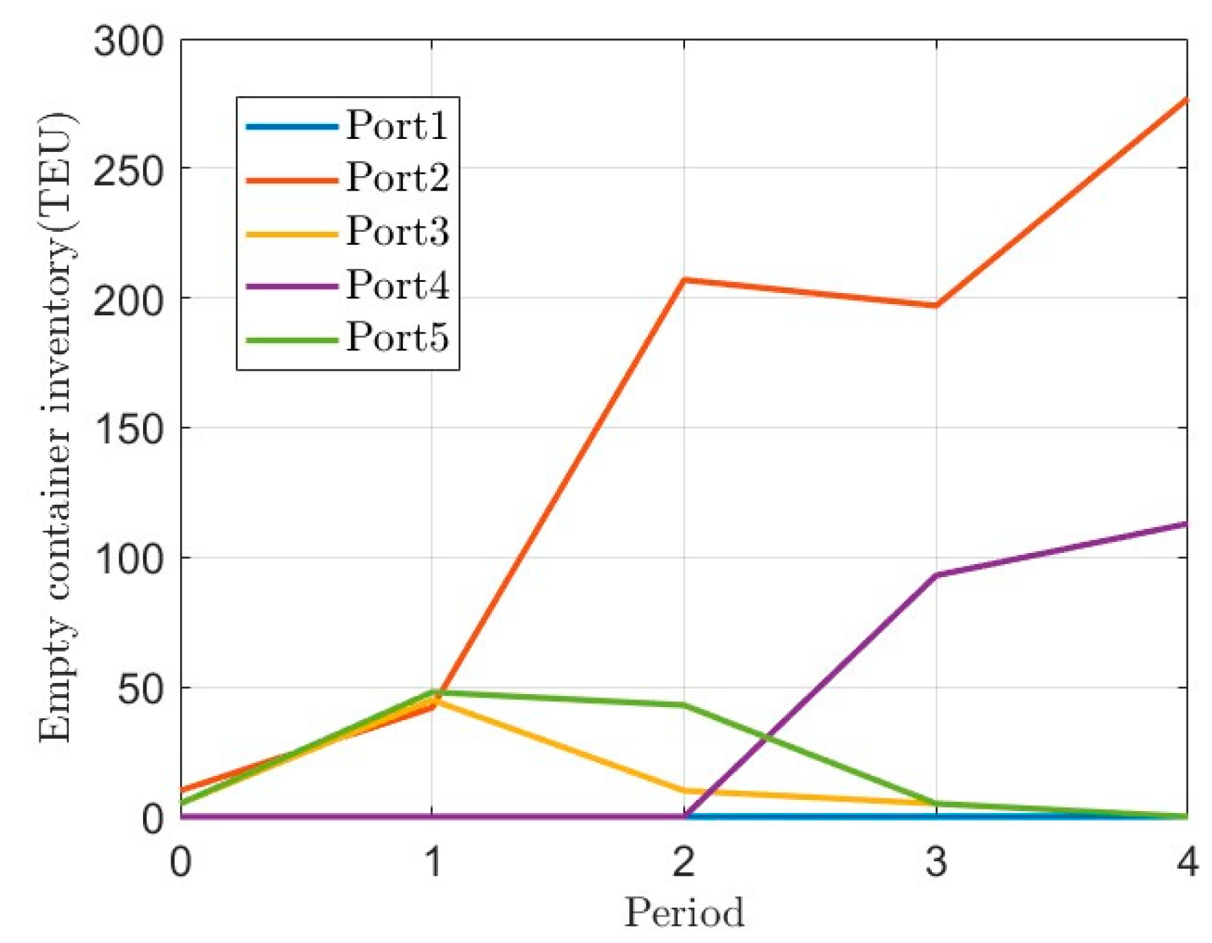
Figure 5 shows the evolution of empty container inventory in each port during different periods.

Firstly, from the convergence graph, the APSO algorithm designed in this paper has good convergence, and the design of heuristic rules for empty container repositioning makes it more suitable for the characteristics of the problem. Secondly, from the calculation results, the application of the (s, S) inventory control strategy can control the rental cost of each cycle at a relatively balanced level. This strategy enables each port to maintain a certain amount of empty container inventory in each decision-making cycle, which can be used to meet empty container demand or temporary empty container demand. From Figure 5, it can also be observed that the empty container inventory at Port 1 remains at 0, indicating that it is in a state of container shortage. The empty container inventory is used to meet the demand for empty containers while also requiring internal container leasing. Port 4 was mostly in a state of shortage of containers in the first two cycles but later achieved a reasonable inventory range of empty containers through container leasing and adjustment. Finally, from the optimal path results, it can also be seen that the flow of empty containers is from surplus container ports to shortage container ports, avoiding reverse transportation from container shortage ports to container surplus ports.

6.3. Sensitivity Analysis

To verify the impact of parameter settings on the various costs, this paper selects three factors for sensitivity analysis, namely unit container rental cost, unit inventory cost, and maximum port inventory capacity.

(1)

Changes in unit rental cost

The unit rental cost accounts for over 60% of the total cost of empty container management, making it crucial for controlling the overall cost of empty container management. Therefore, we calculate and analyze various scenarios where the unit rental cost increases from 20% to 100% in order to explore the relationship between unit rental cost and total cost. The calculation result is shown in Figure 6.

As shown in Figure 6, the cost of empty container management increases with the increase in unit rental cost, and the two are positively correlated. At the same time, it can be observed that regardless of the magnitude of the change, the total cost of renting a container will account for over 60% of the total cost and even reach 80%. Through this experiment, it was found that for shipping companies, the cost of renting is much higher than that of repositioning and inventory. Although renting containers is inevitable, it is also necessary to reduce the renting volume through their own empty container inventory.

(2)

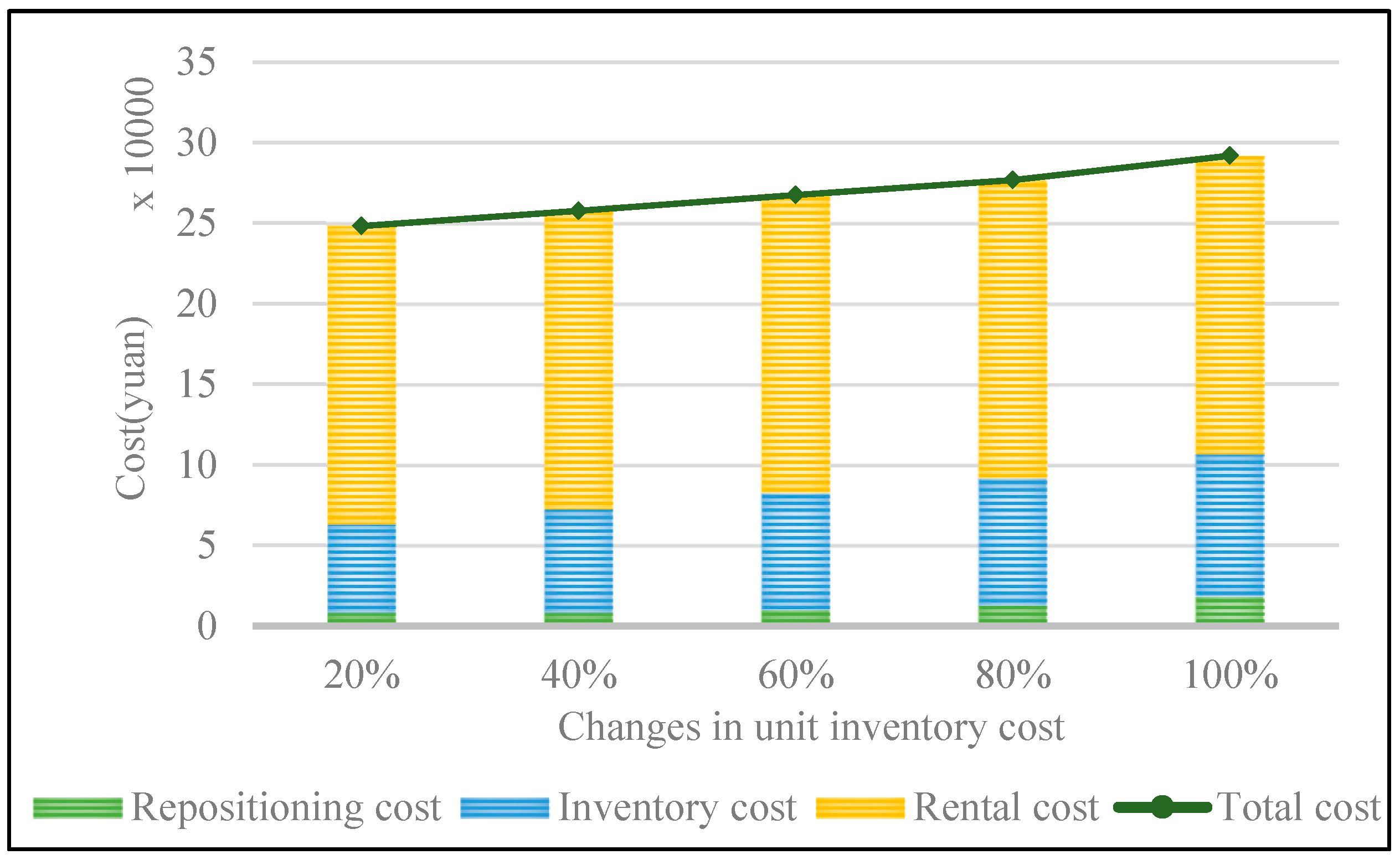
Changes in unit inventory cost

We conducted experiments to increase the unit inventory cost by 20–100%, similar to the unit rental cost. The results are shown in Figure 7. The calculation results demonstrate a positive correlation between the total cost of empty container management and the unit inventory cost. Due to the use of the (s, S) strategy, the inventory level of the shipping company at the port increases, and the increase in unit empty container inventory cost will further exacerbate the inflation of total inventory cost.

(3)

Changes in the maximum inventory capacity of the port

The maximum inventory capacity of a port is the fundamental guarantee for the implementation of the (s, S) strategy, and the setting of (s, S) is closely related to its value, which is the upper limit of the inventory threshold setting. The inventory of empty containers at the same port varies among different shipping companies. Therefore, to explore the relationship between the maximum inventory capacity of empty containers at the port and the total cost of empty container management, we conducted sensitivity experiments by reducing the initial maximum inventory capacity value by 20%–100%. The results are shown in Figure 8.

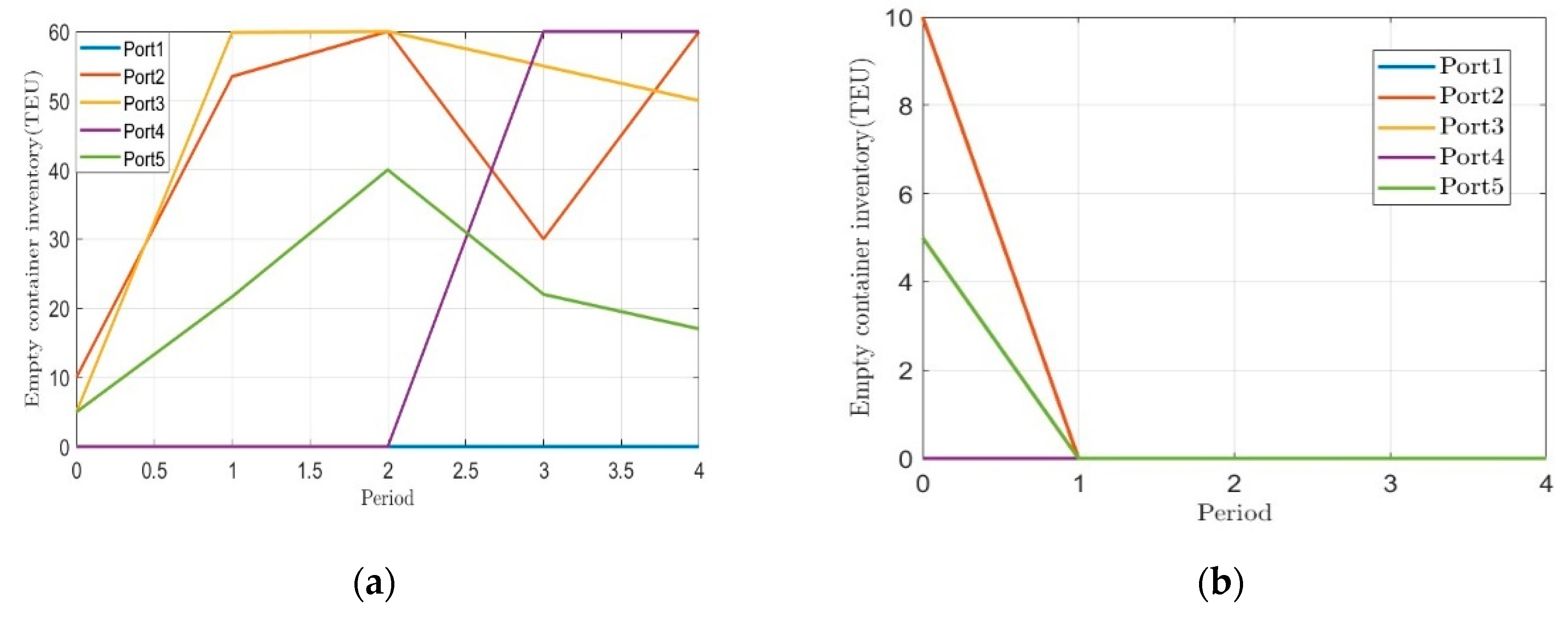
From the calculation results, we can see that during the process of reducing by 20% to 60%, the total cost of empty container management continues to increase. Due to the reduction in port inventory capacity, the cost of repositioning increases. However, it can be observed that the cost of renting containers does not change. This is because by implementing the (s, S) strategy to maintain a stable rental volume, shipping companies can meet the demand for empty containers by increasing the number of container adjustments. When the maximum inventory capacity of the port is reduced to 80%, its inventory capacity can no longer meet the current inventory needs. In the APSO algorithm, due to insufficient port inventory, a truncation situation has occurred. When reduced to 100% and the port has no inventory capacity, the total cost of empty container management has become a huge number due to the existence of the penalty function. Figure 9 shows the inventory evolution of each port under 80% and 100% changes.

Therefore, for shipping companies, limited storage capacity will directly lead to an underground utilization of their empty container resources, while the cost will also increase infinitely. Actively expanding storage space is another new way to solve the high cost of empty container repositioning. Maintaining a good working relationship with the port and striving for more space and time to retain empty containers in the yard will help reduce the costs associated with empty containers.

7. Conclusions

This study proposes a collaborative decision-making framework based on APSO for the collaborative optimization problem of multi-period empty container repositioning and inventory control. Integrating (s, S) inventory control strategy and dynamic repositioning optimization models effectively balances the operating costs, resource utilization, and path planning of the maritime industry.

The main conclusions are as follows:

• Model effectiveness verification: By constructing a collaborative optimization model for empty container repositioning and inventory control, the $\left(s,S\right)$ inventory control strategy is used to synergistically optimize the empty container repositioning path, achieving dynamic collaboration between inventory control and repositioning decisions and verifying the superiority of the “inventory-repositioning” collaborative mechanism.
• Algorithm performance improvement: The designed APSO algorithm dynamically adjusts the inertia weight and acceleration coefficient (inertia weight linearly decays from an initial value of 0.9 to 0.4) and effectively reduces the search space by setting heuristic rules such as surplus and shortage container ports based on the determination of port container volume. The algorithm is closer to the practical characteristics of empty container repositioning and significantly improves global search ability in high-dimensional decision spaces.
• Management insights and sensitivity analysis: The unit rental cost has the most significant impact on the total system cost, indicating that increasing self-owned inventory and container adjustment can effectively reduce rental costs. The sensitivity of the maximum inventory capacity of the port is secondary, and it is recommended that shipping companies prioritize expansion in hub ports to alleviate the pressure of transportation and storage.

Limitations and prospects: The current research assumes that demand disturbances are known, and in the future, deep learning techniques can be combined to achieve dynamic prediction of uncertainty. In addition, the model did not consider multi-agent game behavior (such as competition between ports), and evolutionary game theory will be introduced to further expand it in the future. In addition, from a broader perspective of job prospects, combining the model proposed in this paper with contemporary big data technology and Internet of Things technology can achieve cooperation and coordination at the port level through real-time data interaction.

References

- Xu, X.F.; Huang, X.R.; Wang, L.J. Empty container repositioning problem using a reinforcement learning framework with multi-weight adaptive reward function. Marit. Policy Manag. 2024, 51, 1742–1763. [Google Scholar] [CrossRef]
- Cai, M.; Li, H.; Guo, Z.; Lu, S. Data-driven empty container repositioning for large scale railway network with fuzzy demands. IEEE Trans. Fuzzy Syst. 2023, 31, 557–570. [Google Scholar] [CrossRef]
- Tao, X.Z.; Wu, Q. Energy consumption and CO2 emissions in hinterland container transport. J. Clean. Prod. 2021, 279, 123394.1–123394.13. [Google Scholar] [CrossRef]
- Francesco, M.D.; Lai, M.; Zuddas, P. Maritime repositioning of empty containers under uncertain port disruptions. Comput. Ind. Eng. 2013, 64, 827–837. [Google Scholar] [CrossRef]
- Lin, D.Y.; Juan, C.J. A Bilevel Mathematical Approach for the Empty Container Repositioning Problem with a Sharing and Exchanging Strategy in Liner Shipping. J. Mar. Sci. Technol. -Taiwan 2021, 29, 403–414. [Google Scholar] [CrossRef]
- Xiang, X.; Liu, C.; Jia, S. Tactical vessel deployment and empty container repositioning considering container turnover times. Comput. Ind. Eng. 2024, 190, 110032. [Google Scholar] [CrossRef]
- Numa-Navarro, I.; Wilmsmeier, G.; Gil, C. Improving empty container management using street-turn: A case study of the Columbian logistic network. J. Transp. Geogr. 2023, 112, 103709. [Google Scholar] [CrossRef]
- Tang, Y.; Chen, S.; Feng, Y.; Zhu, X. Optimization of multi- period empty container repositioning and renting in China Railway Express based on container sharing strategy. Eur. Transp. Res. Rev. 2021, 13, 42. [Google Scholar] [CrossRef]
- Jeong, Y.; Saha, S.; Chatterjee, D.; Moon, I. Direct shipping service routes with an empty container management strategy. Transp. Res. Part E 2018, 118, 123–142. [Google Scholar] [CrossRef]
- Lu, T.; Lee, C.Y.; Lee, L.H. Coordinating Pricing and Empty Container Repositioning in Two-Depot Shipping Systems. Transp. Sci. 2020, 54, 1697–1713. [Google Scholar] [CrossRef]
- Furió, S.; Andrés, C.; Adenso-Díaz, B.; Lozano, S. Optimization of empty container movements using street-turn: Application to Valencia hinterland. Comput. Ind. Eng. 2013, 66, 909–917. [Google Scholar] [CrossRef]
- Liang, J.; Ma, Z.; Wang, S.; Liu, H.; Tan, Z. Dynamic container slot allocation with empty container repositioning under stochastic demand. Transp. Res. Part E 2024, 1487, 103603. [Google Scholar] [CrossRef]
- Mehrzadegan, E.; Ghandehari, M.; Ketabi, S. A joint dynamic inventory-slot allocation model for shipping using revenue management concepts. Comput. Ind. Eng. 2022, 170, 108333. [Google Scholar] [CrossRef]
- Rajeswari, S.; Sugapriya, C.; Nagarajan, D.; Broumi, S.; Smarandache, F. Octagonal fuzzy neutrosophic number and its application to reusable container inventory model with container shrinkage. Comput. Appl. Math. 2021, 40, 308. [Google Scholar] [CrossRef]
- Luo, T.; Chang, D.F. Empty container repositioning strategy in intermodal transport with demand switching. Adv. Eng. Inform. 2019, 40, 1–13. [Google Scholar] [CrossRef]
- Poo, M.C.P.; Yip, T.L. An optimization model for container inventory management. Ann. Oper. Res. 2019, 273, 433–453. [Google Scholar] [CrossRef]
- Sarmadi, K.; Amiri-Aref, M.; Dong, J.-X.; Hicks, C. Integrated strategic and operational planning of dry port container networks in a stochastic environment. Transp. Res. Part B-Methodol. 2020, 139, 132–164. [Google Scholar] [CrossRef]
- Garg, H.; Sugapriya, C.; Rajeswari, S.; Nagarajan, D.; Alburaikan, A. A model for returnable container inventory with restoring strategy using the triangular fuzzy numbers. Soft Comput. 2024, 28, 2811–2822. [Google Scholar] [CrossRef]
- Garg, H.; Rajeswari, S.; Sugapriya, C.; Nagarajan, D. A model for container inventory with a trapezoidal bipolar neutrosophic number. Arab. J. Sci. Eng. 2022, 47, 15027–15047. [Google Scholar] [CrossRef]
- Legros, B.; Bouchery, Y.; Fransoo, J.C. A time-based policy for empty container management by consignees. Prod. Oper. Manag. 2019, 28, 1503–1527. [Google Scholar] [CrossRef]
- Guo, M.; Kong, X.T.R.; Chan, H.K.; Thadani, D.R. Integrated inventory control and scheduling decision framework for packaging and products on a reusable transport item sharing platform. Int. J. Prod. Res. 2023, 61, 4575–4591. [Google Scholar] [CrossRef]
- Yang, R.; Yu, M.; Lee, C.-Y.; Du, Y. Contracting in ocean transportation with empty container repositioning under asymmetric information. Transp. Res. Part E 2021, 145, 102173. [Google Scholar] [CrossRef]
- Kamal, B. The use of fuzzy-bayes approach on the causal factors of empty container repositioning. Mar. Technol. Soc. J. 2021, 55, 20–38. [Google Scholar] [CrossRef]
- Wang, Q.B.; Wang, Z.W.; Zheng, J.F. Joint optimization of inventory and repositioning for sea empty container based on queuing theory. J. Mar. Sci. Eng. 2023, 11, 1097. [Google Scholar] [CrossRef]
- Zhou, S.; Zhuo, X.; Chen, Z.; Tao, Y. A new separable piecewise linear learning algorithm for the stochastic empty container repositioning problem. Math. Probl. Eng. 2020, 2020, 4762064.1–4762064.16. [Google Scholar] [CrossRef]
- Rajeswari, S.; Sugapriya, C.; Nagarajan, D. Fuzzy inventory model for NVOCC’s returnable containers under empty container repositioning with leasing option. Complex Intell. Syst. 2021, 7, 753–764. [Google Scholar] [CrossRef]
- Abdelshafie, A.; Rupnik, B.; Kramberger, T. Simulated global empty containers repositioning us-ing agent-based modelling. Systems 2023, 11, 130. [Google Scholar] [CrossRef]
- Najafi, M.; Zolfagharinia, H. Pricing and quality setting strategy in maritime transportation: Considering empty repositioning and demand uncertainty. Int. J. Prod. Econ. 2021, 240, 108245. [Google Scholar] [CrossRef]
- Lee, S.; Moon, I. Robust empty container repositioning considering foldable containers. Eur. J. Oper. Res. 2020, 280, 909–925. [Google Scholar] [CrossRef]
- Chi, M.; Zhu, X.; Wang, L.; Zhang, Q.; Liu, W. Multi-period empty container repositioning approach for multimodal transportation. Meas. Control 2024, 57, 361–377. [Google Scholar] [CrossRef]
- Siswanto, N.; Wiratno, S.E.; Rusdiansyah, A.; Sarker, R. Maritime inventory routing problem with multiple time windows. J. Ind. Manag. Optim. 2020, 15, 1185–1211. [Google Scholar] [CrossRef]
- Castrellon, J.P.; Sanchez-Diaz, I.; Roso, V.; Altuntas-Vural, C.; Rogerson, S.; Santén, V.; Kalahasthi, L.K. Assessing the eco-efficiency benefits of empty container repositioning strategies via dry ports. Transp. Res. Part D 2023, 120, 103778. [Google Scholar] [CrossRef]
- Shi, X. The study in the optimization of empty container inventory. Navig. China 2002, 1, 59–62. [Google Scholar]