Task-Sequencing Optimization Using DSSA Algorithm for AUV with Limited Endurance

Abstract

Efficiency is very important for robots when executing multiple tasks, especially for autonomous underwater vehicles (AUVs) with limited endurance. In order to improve efficiency, task-sequencing optimization, which focuses on achieving the optimal execution order of multiple tasks, is one effective way. In this paper, the classic lawnmower traverse task is taken as an example for optimization, and discrete salp swarm algorithm (DSSA), which combines salp swarm algorithm (SSA) and genetic algorithm (GA), is selected and applied to optimize task sequencing for one AUV. In the optimization process, there are two key problems that need to be solved. One is how to encode the individual chromosome and the other is how to perform genetic operations on chromosomes of different lengths. For the former problem, a two-layer encoding method is proposed to generate individuals in the population, in which identity number and entry point of different areas are encoded, respectively. For the latter problem, mutation and crossover operators are modified and extended to deal with individuals of variable length due to the limited endurance of AUVs. Simulation results show that the sequencing optimization can be achieved after finite iteration. Through comprehensive comparison, DSSA is finally implemented and verified in a physical AUV.

1. Introduction

Autonomous underwater vehicles (AUVs) are one of the research hotspots in the field of marine equipment development, and they play an irreplaceable role in ocean exploration, mineral investigation, and hydrology surveys with their autonomy and intelligence [1,2,3]. Typically, an AUV carries limited battery power for underwater operations with little human intervention, so how to maximize the efficiency of an AUV autonomously is very meaningful. One of the most effective and intuitive ways to improve efficiency is to optimize the sequence of task execution and achieve certain optimization goals, such as minimizing the planning path length. Moreover, the optimization can also enhance the intelligence of AUVs to adapt to the complex and dynamic environment. Therefore, this paper takes the classic lawnmower traverse task as an example to introduce and verify a task-sequencing optimization method for an AUV, since the lawnmower traverse task is often performed when detecting and collecting marine data [4,5,6]. For a task-sequencing problem, its optimization is similar to the traveling salesman problem (TSP), which is in discrete space and is an NP-Hard problem [7,8]. Generally, there are two solutions to this problem; one is the exact calculation method, and the other is based on a metaheuristic algorithm. The former includes branch and bound [9], branch and cut [10], dynamic programming [11], etc., which can obtain the optimal solution, but the amount of computation increases exponentially as the scale of the problem increases. The latter is mainly represented by an evolutionary algorithm and swarm intelligent algorithm, such as the genetic algorithm (GA) [12], particle swarm algorithm (PSO) [13], ant colony algorithm (ACO) [14], quantum-based avian navigation optimizer algorithm (QANA) [15], nonlinear marine predator algorithm (NMPA) [16], etc. Although the result is sub-optimal using these metaheuristic algorithms, computation complexity does not change significantly with change of problem scale compared with exact calculation method, and in most cases, a sub-optimal solution has met the actual requirements. Therefore, a metaheuristic algorithm is selected for task-sequencing optimization in this paper.

Specifically, discrete salp swarm algorithm (DSSA), which combines salp swarm algorithm (SSA) and genetic algorithm (GA), is selected and applied to optimize task-sequencing for AUV, due to its advantages, such as few parameters and good effect. The algorithm is inspired and improved from discrete salp swarm algorithm (DSSA) for the traveling salesman problem (TSP) [17,18]. For the AUV application scenario of this paper, there are two key problems that need to be solved when using the optimization algorithm based on DSSA. One is how to encode the individual chromosome and the other is how to perform genetic operations on chromosomes of different lengths. The solutions to these two problems are proposed in this paper.

The main contributions of this paper are as follows:

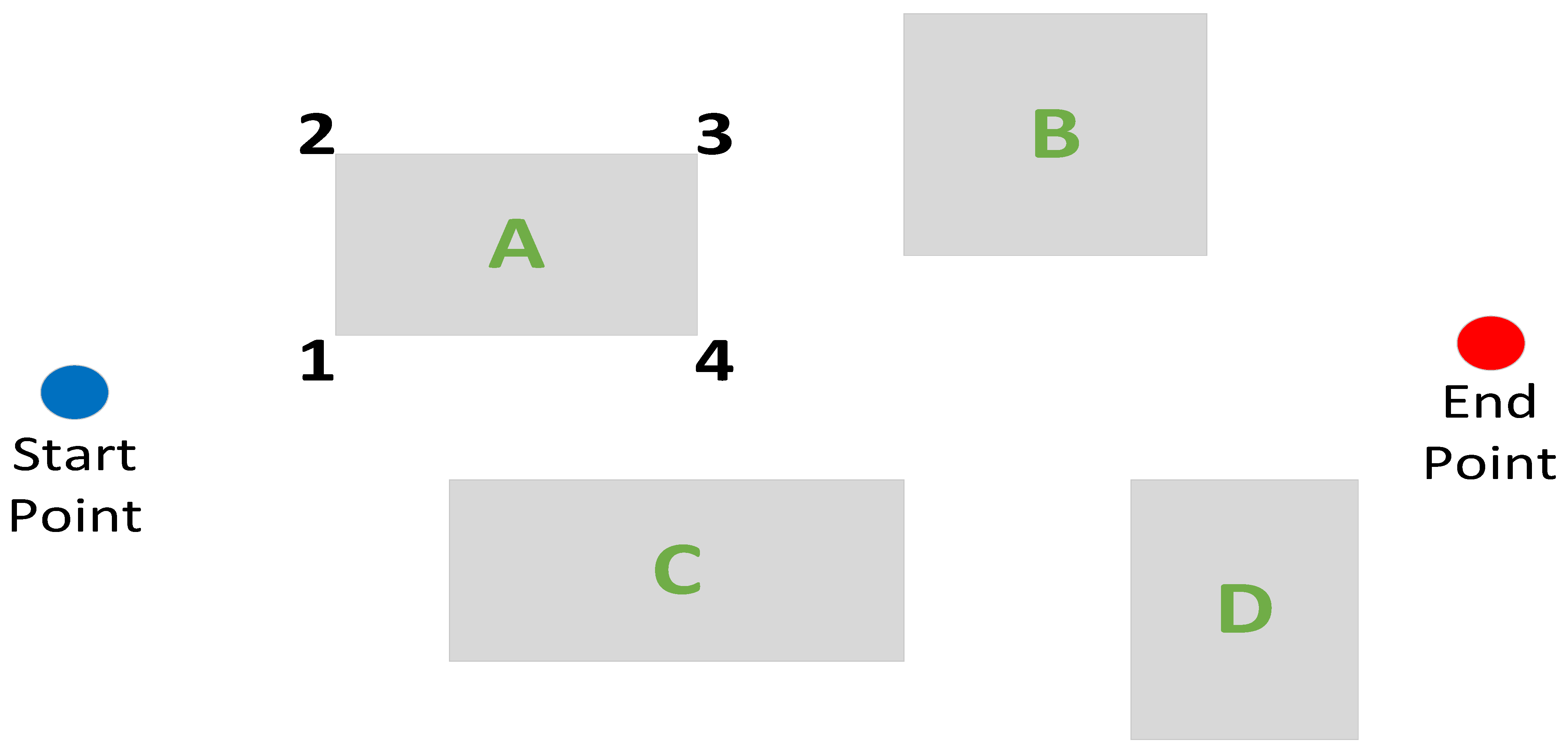
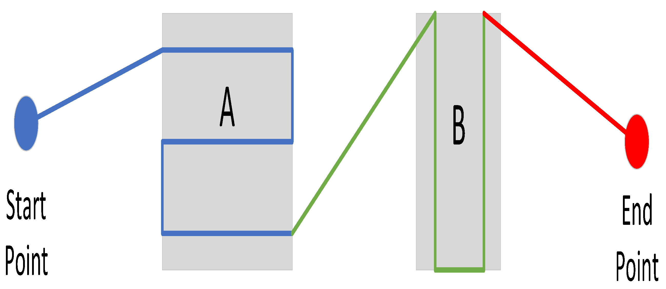
• Considering identity number and entry point of different task areas, a two-layer encoding scheme is proposed for individual chromosomes.
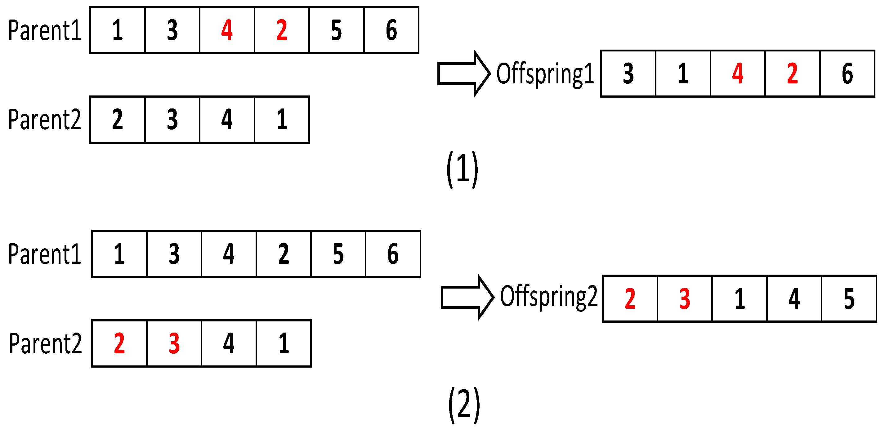
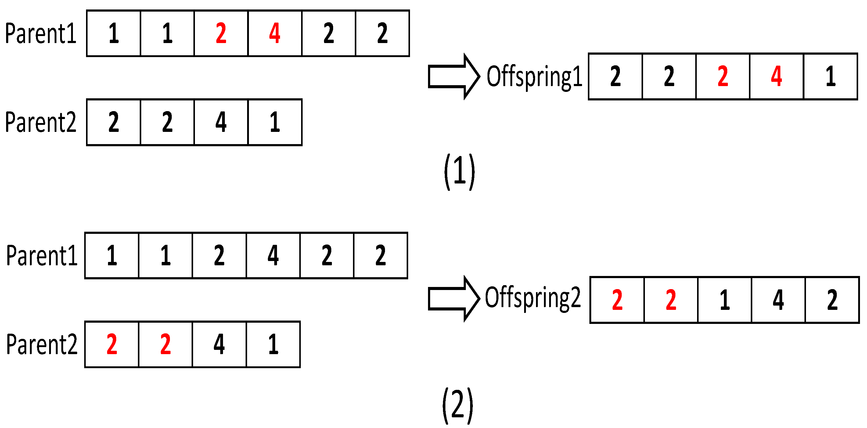
• Due to the constraint of limited endurance of an AUV, genetic operators, such as mutation and crossover operators, are modified and improved to process chromosomes of variable size.
• DSSA is modified and improved for the optimization of lawnmower task sequencing and the algorithm is implemented and verified in a physical AUV.

The rest of the paper is organized as follows. Section 1 introduces the related research work. Section 2 formulates the optimization model, and describes the application of the DSSA algorithm in detail. In Section 3, simulation and experiment results are shown and discussed. Finally, conclusions and future work are given in Section 4.

2. Related Works

Metaheuristic algorithms, represented by the evolutionary algorithm and swarm intelligent algorithm, have been applied to robot task sequencing. As described in [8], metaheuristics have been proved to be efficient for tour-searching problems and, as a consequence, are well-suited for task sequencing in robotics.

GA is a well-known evolutionary algorithm inspired by natural selection and the result is generated from one generation to the next without depending on strict mathematical formulation [19,20]. The GA algorithm has inherently discrete properties and is suitable for problems in discrete space. Therefore, GA has been successfully applied in many fields. For example, GA was used to solve a task-planning problem of manipulator arms, which optimized the joint configuration and end movement path of manipulator arms [21,22]. In [21], each individual adopted a special coding method in which double-layer coding of path-point sequencing and joint configuration was used. In [23], an ant colony optimization (ACO) algorithm was used for the optimization of the industrial robot base layout and robotic task sequence. In [24], particle swarm optimization (PSO) was used to solve the problem of manipulator system selection for a multiple-goal task considering completion time and cost with computational time. However, for the manipulator arm, task-planning optimization is not constrained by battery power, which is different from the scenario of AUVs with limited endurance.

Besides these applications, several studies also investigated the advantages of metaheuristic methods on robot mission management in terms of vehicle routing and task assignment [25]. In [26,27], vehicle-routing problems (VRPs) were classified and the solving algorithms were analyzed. As mentioned in the literature, the evolutionary algorithm represented by GA can approach the optimal solution and shorten the operation time, and it is a promising method. In [28], the GA algorithm was utilized to solve a vehicle-routing problem with simultaneous pick-up and deliveries. In [29], the GA-algorithm-based approach to multi-depot heterogeneous limited fleet VRP with time windows was proposed. However, these studies rarely involve solutions of variable lengths.

For the task allocation of AUVs, there are also some studies on metaheuristic algorithms. In [30,31], L-SHADE algorithm was used to optimize multi-area coverage planning path for AUV, aiming at the shortest path length. The method in the literature focuses on path planning and does not take into account the endurance constraint of AUV. In [7], GA algorithm was used to optimize task sequence in large-scale operation areas. In [32], differential evolution (DE) algorithm was employed for the waypoint sequence generation and mission time management. In addition, other metaheuristic algorithms were also applied to sequence optimization. In [33,34], biogeography-based optimization (BBO) and particle swarm optimization (PSO) were adapted to provide real-time optimal solutions for task sequence selection and mission time management of AUVs. In [35], ACO algorithm was utilized to find an optimum order of tasks for the underwater mission of AUVs. During these optimization processes, the limited endurance of AUVs was considered in a few studies. However, in these studies, tasks were simplified into a network connected by points and the classic lawnmower traverse task was not analyzed. For the lawnmower traverse task, entry points of different areas have a significant impact on total path length when optimizing task-sequencing.

In this paper, discrete salp swarm algorithm (DSSA), which combines salp swarm algorithm (SSA) and GA, is used to optimize traverse task sequencing for AUVs. As a new algorithm proposed in recent years, SSA mimics the swarming behavior of salps and has simple and effective features [36]. In the algorithm, most parameters are random values, which reduces the computational complexity. SSA has been successfully utilized in a wide range of optimization problems in different fields and scenarios, such as machine learning, engineering design, wireless networking, image processing, and power energy [37]. Since the traditional SSA algorithm is used in continuous space, it needs to be modified in discrete space by some methods, such as combining genetic operators. For example, in [38], hybrid salp swarm algorithm and genetic algorithm (HSSAGA) was used to optimize the allocation of nurses to COVID-19 patients. And in [17,18], DSSA combined with genetic operators was introduced for the traveling salesman problem. In [39], manta ray foraging optimization (MRFO) and SSA were discretized using GA to solve controller placement problem (CPP) in software defined network (SDN). In [40], an enhanced opposition-based learning salp swarm algorithm (EOSSA) was presented for solving the feature selection (FS) problem in intrusion detection systems (IDSs). However, these existing discrete SSA algorithms cannot be used to solve the problems for the scenario with variable length of each individual solution. In this paper, the improved DSSA, which combines SSA and GA, is proposed for the scenario.

3. Materials and Methods

3.1. Formulation of Task-Sequencing for an AUV

3.1.1. Mathematical Representation of Operating Areas

This paper focuses on the optimization of execution sequence of multi-area traverse tasks. In the scenario, there are N areas which are numbered from 1 to N and an AUV moves at the same depth in these areas. In the example shown in Figure 1, there are four rectangular areas and an area has four vertices whose identity numbers are from 1 to 4. One rectangular area represents one traverse task. And an AUV executes these tasks from the blue start-point, traverses multiple areas, and finally reaches the red end-point. The desired depth is fixed during AUV operation.

When traversing an area, an AUV typically follows a lawnmower path. The distance between two adjacent parallel lines which are known as survey lines in the path, depends on the detection range of onboard sensors, such as Side Scan Sonar (SSS). In order to reduce the number of turns, survey lines are normally planned along the long side of an area.

As shown in Figure 2, there are four kinds of lawnmower path from different entry points of a task area. The blue circle indicates the position of entry-point and the red one is exit-point. Entry-point is associated with the vertices of a task area, and exit-point is determined after path planning. Different entry points have an impact on the total path length, especially the path length between different tasks. Therefore, the impact of entry-point is considered for task-sequencing optimization in this paper.

3.1.2. Mathematical Representation of Task-Sequencing for an AUV

Typically, an AUV is powered by a battery and its endurance is limited. Therefore, the optimization goal is to execute as many tasks as possible with limited endurance. Assume that the number of tasks is $N_a$.

$$\begin{array}{cc}\hfill & N_a=\sum _{j=1}^N{l}^j,l^j\in \left\{0,1\right\}\hfill \\ \hfill & N_r=N-N_a\hfill \end{array}$$

(1)

$l^j$ is the selection status of the jth task, where 1 indicates that the task is selected to be traversed and 0 means that the task is not to be executed. $N_r$ is the number of remaining tasks which are not executed.

The total length of the path planned is shown as follows.

$$D_t=d_e+\sum _{j=1}^N{l}^j{d}^j,l^j\in \left\{0,1\right\}$$

(2)

where $d^j$ is the sum of the distance from start-point to entry-point of the jth area and length of paths planned using lawnmover mode in the jth area. $d_e$ is the distance from exit-point of the last area to end-point. In the example shown in Figure 3, $d^1$ is the total path length of the first area marked by the blue line and $d^2$ is the total path length of the second area represented by the green line. And $d_e$ is the distance from exit-point of the second area to end-point marked by the red line.

As mentioned above, the optimization goal is to execute as many tasks as possible with the limited endurance of an AUV. And the goal can be translated into minimizing the remaining tasks before endurance exhaustion. Assuming that the benefit of the ith task is $b^i$, the total benefits of the remaining tasks are shown as follows.

$$B_r=\sum _{i=1}^{N_r}{b}^i$$

(3)

Therefore, the objective function can be changed to single-object form by the following expression, which indicates the fitness value of an individual solution during optimization.

$$F=w_{1}log(B_r+1)+w_{2}log(D_t+1)$$

(4)

where $w_1$ and $w_2$ represent the weight value. And since the number range of path length and benefit are different, the logarithmic function is used for normalization. Moreover, to avoid negative values for the logarithmic function, path length and benefit are increased by one, respectively, in Equation (4).

Finally, the optimization goal is to minimize the fitness value, as shown below.

$$\begin{array}{c}Min\left(w_{1}log(B_r+1)+w_{2}log(D_t+1)\right)\hfill \\ s.t.D_t\le D_{available}\hfill \end{array}$$

(5)

where the total path length $D_t$ is constrained by the maximum endurance $D_{available}$. Considering the endurance limit, a penalty is added to the fitness value. When the total path length exceeds the endurance, the fitness takes a relatively large value.

The mathematical notations in the model of task-sequencing for an AUV are listed in

Table 1. Mathematical notations list.

Mathematical Notation	Explaination
N	Number of tasks
$N_a$	Number of executed tasks
$N_r$	Number of unexecuted tasks
$l^j$	Selection status of jth task
$D_t$	Length of total paths
$d^j$	Length of path for jth task
$D_{available}$	Endurance of AUV
$B_r$	Total benefits of unexecuted tasks
$b^i$	Benefit of ith task
F	Fitness value of an individual solution
$w_1$	Weight value of benefits for unexecuted tasks
$w_2$	Weight value of total path length

.

3.2. Task Sequencing Process

3.2.1. Overview of DSSA

SSA is inspired by the swarming behavior of salps and the population is divided into two groups: leader and follower [36]. The leader is the salp at the front of the chain which guides the swarm, whereas the rest of the salps are considered as followers which follow each other. The position of the leader is updated using the following expression:

$$x_j^l=\left\{\begin{array}{c}{F}_j+c_1\left(\left(u{b}_j-l{b}_j\right)c_2+l{b}_j\right)c_3\ge 0.5\hfill \\ F_j-c_1\left(\left(u{b}_j-l{b}_j\right)c_2+l{b}_j\right)c_3<0.5\hfill \end{array}\right.$$

(6)

where $x_j^1$ shows the position of the leader salp in the jth dimension, $F_j$ is the position of the food source in the jth dimension, $u{b}_j$ indicates the upper bound of the jth dimension, $l{b}_j$ indicates the lower bound of the jth dimension, $c_2$ and $c_3$ are random numbers. The coefficient $c_1$ is used to balance exploration and exploitation and is defined as follows:

$$c_1=2e^{-{\left({\displaystyle \frac{4l}{L}}\right)}^2}$$

(7)

where l is the current iteration and L is the maximum number of iterations. The parameters $c_2$ and $c_3$ are random numbers uniformly generated in the interval of [0, 1]. These parameters dictate if the next position in the jth dimension should be towards positive infinity or negative infinity as well as the step size. The position of the follower is updated using the following equations:

$$x_j^i={\displaystyle \frac{1}{2}}\left(x_j^i+x_j^{i-1}\right)$$

(8)

where $i\ge 2$ and $x_j^i$ shows the position of the ith follower salp in the jth dimension.

From the above introduction, it can be seen that the parameters of SSA are few and mostly random values, giving it the characteristics of convenient use, simple logic and fast convergence. However, the classical SSA works in continuous space. It is difficult to apply directly to solving problems in discrete space. An effective way is to combine the algorithm with discrete operators, i.e., DSSA, which is suitable for discrete problems [17,18]. From these two studies, it can be seen that DSSA has more advantages for TSP-type problems compared with other algorithms, such as good effect, fast convergence, and few parameters. However, these existing DSSA algorithms cannot be used to solve the problems for the scenario in which the length of each individual solution is variable. In this paper, the improved DSSA, which combines SSA and GA, is proposed. In GA algorithm, there are three kinds of operators, i.e., selection, mutation, and crossover. Firstly, a population of solutions, known as chromosomes, is initialized. And then parents are selected from the population in each iteration according to their fitness values, and combined through a crossover operator to generate offspring. Moreover, a mutation operator is applied to ensure the diversity of the population. Finally, competitive solutions are selected as parents in the next iteration.

In the proposed DSSA, the main combination of SSA and GA is to update the leader by the mutation operator and the follower by the crossover operator. In the following sections, the optimization process is introduced from the aspects of individual encoding, selection, mutation and crossover operators.

3.2.2. Individual Encoding

From the previous introduction, it can be seen that the total path length is determined by task sequence, entry and exit points of each task area. Therefore, a two-layer encoding approach is proposed to define an individual chromosome, in which the first layer represents the task area sequence and the second layer indicates the selection of entry points of each task area. The reason why only the entry point is used is that one entry point corresponds to one exit point after planning the path.

For N tasks, one execution sequence is shown as below.

$$\left\{A_1,A_2,A_3,...,A_j\right\}j\in \left[1,N\right]$$

(9)

where $A_j$ is the identity number of the jth task. And the number is unique for each task. For example, when there are 4 tasks, the execution sequence can be $\left\{1,2,3\right\}$ or $\left\{2,1,3\right\}$ or $\left\{4,2,1,3\right\}$.

Since there are 4 entry points in each task area, one set of entry points is shown as the following.

$$\left\{E_1,E_2,E_3,...,E_j\right\}{E}_j\in \left[1,4\right],j\in \left[1,N\right]$$

(10)

where $E_j$ is the entry-point number of the jth task area. And the number can be the same for different areas. It is noteworthy that the length of the task sequence and corresponding entry-point sequence should be equal. For example, if there is one task sequence $\left\{2,1,3\right\}$, the corresponding entry-point sequence is $\left\{1,1,2\right\}$. In the initialization before optimization, each individual chromosome is generated randomly and the length of each individual is also variable.

3.2.3. Selection Operation

Through the selection operation, individual chromosomes with better fitness can be preserved, which is conducive to obtaining the optimal individuals. There are some selection operators, such as roulette selection, ranking selection and tournament selection. In this paper, tournament selection is used, in which a group of individuals are randomly selected and then the individual with the best fitness is the winner.

3.2.4. Mutation Operation

Mutation operation is used to update individual chromosomes and is beneficial to enhance the exploration of optimization. In this paper, the mutation is operated to update the leader. Mutation operators including insertion, deletion, inversion, swap and replacement are all utilized and the mutation type is determined randomly. The mutation degree $n_m$ depends on $c_1$ and $c_2$ according to the following formula.

$$n_m=⌊{\displaystyle \frac{1}{2}}\left(c_1{c}_2\right)N⌋$$

(11)

where N is the total number of tasks. $n_m$ is assigned to 1 if it is smaller than 1 and its maximum value is limited to N. Furthermore, $n_m$ represents the number of operations for the mutation operator. For example, in inversion operation, $n_m$ means the length of the inverted segment in an individual chromosome, but it can not be larger than the size of an individual. In the early stage of optimization, the larger value of $n_m$ can enhance the exploration, and in the later stage, the smaller value is conducive to convergence.

3.2.5. Crossover Operation

In this paper, crossover operation is performed between two individual chromosomes which involve task sequence and entry-point sequence. And order crossover (OX) is selected for this operation, since the ordered gene sequence is preserved and gene values are not duplicated in OX operation, which is suitable for optimization problems similar to TSP [41]. Specially, $O{X}_3$, which is a variation of traditional order crossover, is utilized for crossover operation [42]. Considering the variable length of the individual chromosome, $O{X}_3$ is modified. One of the modifications is that the size of the chromosome segment from parents is half the length of the shorter individual chromosome during crossover operation. And another modification is that sequence length of the offspring is half the sum of the sequence length of parents according to Equation (8). An example is shown in Figure 4.

In this example, the red numbers are selected as the segment from a parent sequence during $O{X}_3$ crossover operation. By combining the segment and elements from the other parent, offspring sequences are born. And the length of the offspring sequence, which is 5, is half the sum length of parents, which is 10. If the length of a parent sequence is less than offspring, the remaining tasks are randomly selected to complement offspring. For example, the element marked as 6 in Offspring1 is randomly selected from identity numbers of the remaining tasks.

The example of crossover operation for the entry-point sequence is shown in Figure 5. One important difference from the task sequence is that the elements can be duplicated in an entry-point sequence. After selecting the chromosome segment from a parent, elements are randomly selected from the other parent to supplement the offspring sequence.

3.2.6. Overall Process of the Proposed DSSA

The overall process of the proposed DSSA algorithm is shown as Figure 6.

The overall peseudocode of the DSSA algorithm proposed in this paper is shown as below. According to Algorithm 1, the computational complexity is $O(T\times N\times D^2)$, where T represents the maximum number of iterations, N indicates the size of the population and D is the dimension of a solution. In the worst case, the complexity of $O{X}_3$ crossover operation is $O\left(D^2\right)$ for two individual solutions of the same size as the number of tasks.

Algorithm 1:Task-sequencing peseudocode using the proposed DSSA

Input: Start-point $P_s$; End-point $P_e$; A set of task areas containing entry-point, exit-point and the planned path. Output: The optimized task sequence $O{S}_t$; The optimized entry-point sequence $O{S}_e$ 1: Initialization: Number of individuals $N_v$; Maximum iterations $I_m$ 2: for $i=1$ to $N_v$ do 3:     Randomly generated individual task sequences $I{S}_t$ 4:     Randomly generated individual entry-point sequences $I{S}_e$ 5:     Calculate the fitness value of individuals based on Equation (4) 6: end for 7: Update food position based on fitness value using Formula (5) 8: The task sequence corresponding to food position $I{S}_t^f$ 9: The entry-point sequence corresponding to food position $I{S}_e^f$ 10: while  $N\le I_m$  do 11:     Update $c_1$ based on Equation (7) 12:     for $j=1$ to $N_v$ do 13:         $c_2\leftarrow rand\left(\right)$ 14:         $c_3\leftarrow rand\left(\right)$ 15:         if $j\le {\displaystyle \frac{N_v}{2}}$ then 16:            Calculate the mutation degree using Equation (11) 17:            Select mutation operation according to the value of $c_3$ 18:            Execute mutation operation based on food position: $I{S}_t^f$ and $I{S}_e^f$ 19:            Update leader position according to mutation result 20:         else 21:            Execute $O{X}_3$ crossover operation between $I{S}_t^{j-1}$ and $I{S}_t^j$ 22:            Execute $O{X}_3$ crossover operation between $I{S}_e^{j-1}$ and $I{S}_e^j$ 23:            Update follower position according to crossover result 24:         end if 25:         Calculate the fitness value of individual based on Equation (4) 26:     end for 27:     Update food position based on fitness values using Formula (5) 28: end while

4. Results

This section discusses and analyzes the application results of DSSA from the perspectives of the simulation and lake experiment. Before the lake experiment, the task-sequencing process was simulated in Matlab2019B. In the simulation, GA was selected and compared with DSSA in this paper, since it has been successfully applied and verified in many task-sequencing problems. When applying GA in task-sequencing of AUV, similar improvement methods proposed in the paper were used, such as the methods of individual encoding and crossover operation.

4.1. Simulation Results

4.1.1. Simulation Results Using GA

In GA algorithm simulation, the number $I_m$ of iterations is 300 and the population size $N_v$ is 100. Besides that, there are also some other parameters, such as the number of mutated bits $n_m$, mutation rate $R_m$ and crossover rate $R_c$. The values of these parameters are shown in

Table 2. Parameters in GA simulation.

Parameter Name	Value
Iterations $I_m$	300
Population $N_v$	100
Mutation bits $n_m$	2
Mutation rate $R_m$	0.5
Crossover rate $R_c$	1

. In the simulation, scenarios with 8 tasks and 20 tasks whose locations are randomly distributed in the map are taken as examples, and the endurance mileage of an AUV is 10 km. The performance metrics of two scenarios are listed in

Table 3. Performance metrics for 8 areas and 20 areas in GA simulation.

Performence Metrics	Senario1	Senario2
Number of areas	8	20
Endurance (km)	10	10
Computation time (s)	4.3018	5.6647
Best fitness	0.1989	2.3421
Total distance (km)	9.647	9.506
Remaining mileage (km)	0.353	0.494
Covered areas	8	8
Remaining areas	0	12

and the evolution curve is shown in Figure 7. The parameters in the simulation are set as follows: $n_m$−2, $R_m$−0.5, $R_c$−1. From the result, it can be seen that whether the path length exceeds the endurance or not, the algorithm can optimize the task-sequencing after finite iterations. When the number of tasks is 8, there are no remaining areas because the total length of the planned path (9.647 km) is less than the endurance (10 km). When the number is 20, there are 12 areas left because of the limited endurance of the AUV. Although the dimension of optimization space is changed from 8 to 20, the computation time increases by just over one second.

Figure 8 shows the planning trajectory after optimization in the simulation. In the diagram, the task areas are represented by blue rectangles and the planning trajectory is marked with a red line. And each task area is identified by a green identity number. The side length of one grid in the figure is 50 m and the distance between survey lines is 100 m. The point marked with “Begin” is the start-point of the AUV and the point marked with “End” is the end-point. In the 8-area scenario, the optimized task sequence is 8-2-5-6-7-4-1-3. The entry-point for each area is 1-1-1-1-1-1-4-2. In the 20-area scenario, the optimized task sequence is 17-1-7-4-14-8-5-3 and the entry-point for each area is 1-4-4-1-1-4-1-4.

The box plot of statistic data for the scenario with 20 areas after 100 executions of the GA simulation is shown in Figure 9 and the key metrics of box plots are listed in

Table 4. Statistic data for 20 areas in GA simulation.

Performance Metrics	Q1	Median	Q3	Interquartile	Minimum	Maximum
Best fitness	2.3412	2.3641	2.3681	0.0269	2.3374	2.3954
Computation time (s)	5.1998	7.0548	9.9312	4.7314	2.9963	14.9189
Total distance (km)	7.6913	8.3922	9.122	1.4307	6.271	9.7885
Covered areas	7	7	8	1	6	8

. From the statistics, it can be seen that although computation time and total distance have a significant volatility, the value of best fitness and the number of covered areas have a certain stability.

4.1.2. Simulation Results Using DSSA

During the simulation of DSSA, the number $I_m$ of iterations is set to 300 and the population size $N_v$ is 100. The other parameters in DSSA, such as $c_2$ and $c_3$, are generated randomly. The parameters of DSSA are shown in

Table 5. Parameters in DSSA simulation.

Parameter Name	Value
Iterations $I_m$	300
Population $N_v$	100
$c_1$	Determined by iterations
$c_2$	Random number
$c_3$	Random number

. In the simulation, scenarios with 8 tasks and 20 tasks are also taken as examples, and the endurance mileage of AUV is 10 km. The performance metrics of two scenarios are listed in

Table 6. Performance metrics for 8 areas and 20 areas in DSSA simulation.

Performance Metrics	Scenario1	Scenario2
Number of areas	8	20
Endurance (km)	10	10
Computation time (s)	4.3413	6.815
Best fitness	0.1990	2.3419
Total distance (km)	9.6745	9.472
Remaining mileage (km)	0.3255	0.528
Covered areas	8	8
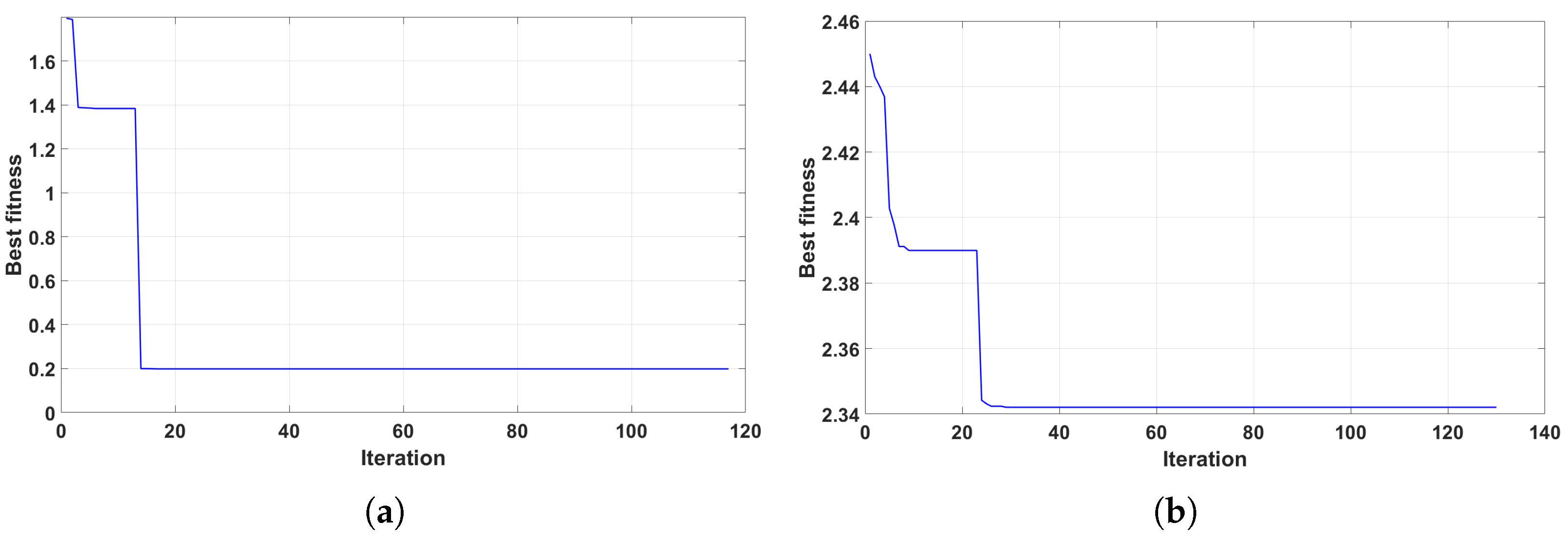
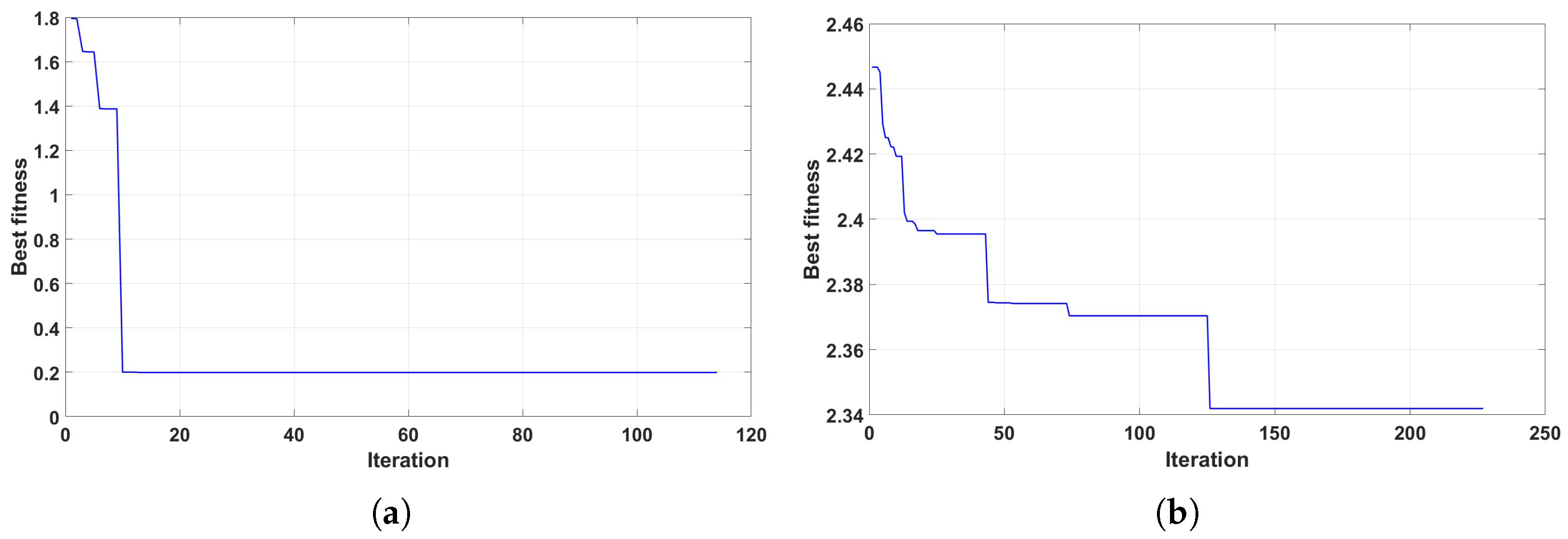
Remaining areas	0	12

and the evolution curve is shown in Figure 10. From the result, it can be seen that the algorithm can optimize the task-sequencing after finite iterations. When the number of areas is 8, the total length of the planned path is 9.6745 km, which is less than the endurance (10 km). When the number is 20, there are 12 areas left and the total path length is 9.472 km. Compared with GA, DSSA performs similarly in a single simulation.

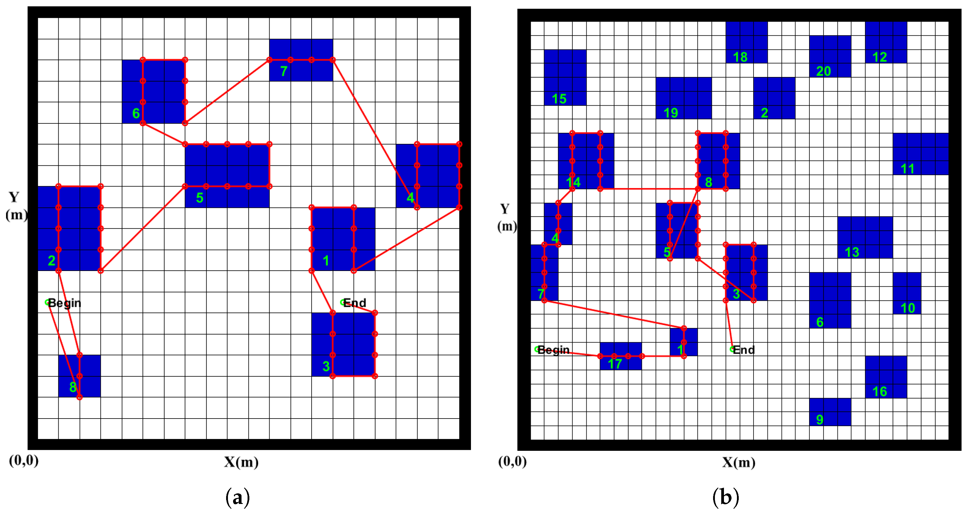
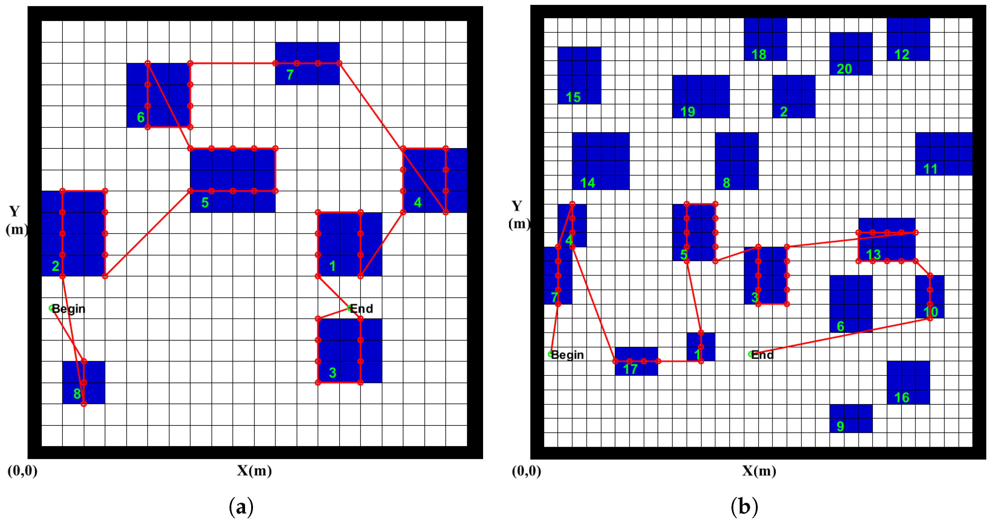
Figure 11 shows the planning trajectory after optimization for DSSA. In the 8-area scenario, the optimized task sequence is 8-2-5-6-7-4-1-3. The entry-point sequence is 3-1-1-2-2-4-4-3. Compared with GA algorithm, the task sequence is the same and entry-point sequence is different. According to the value of best fitness, the result obtained by GA algorithm, whose fitness value is 0.1989, is slightly better than DSSA, whose fitness value is 0.1990. In the 20-area scenario, the optimized task sequence is 7-4-17-1-5-3-13-10 and the entry-point sequence is 4-2-2-4-1-2-3-2. According to value of the best fitness, the result obtained by DSSA algorithm, whose fitness value is 2.3419, is better than GA algorithm, whose fitness value is 2.3421.

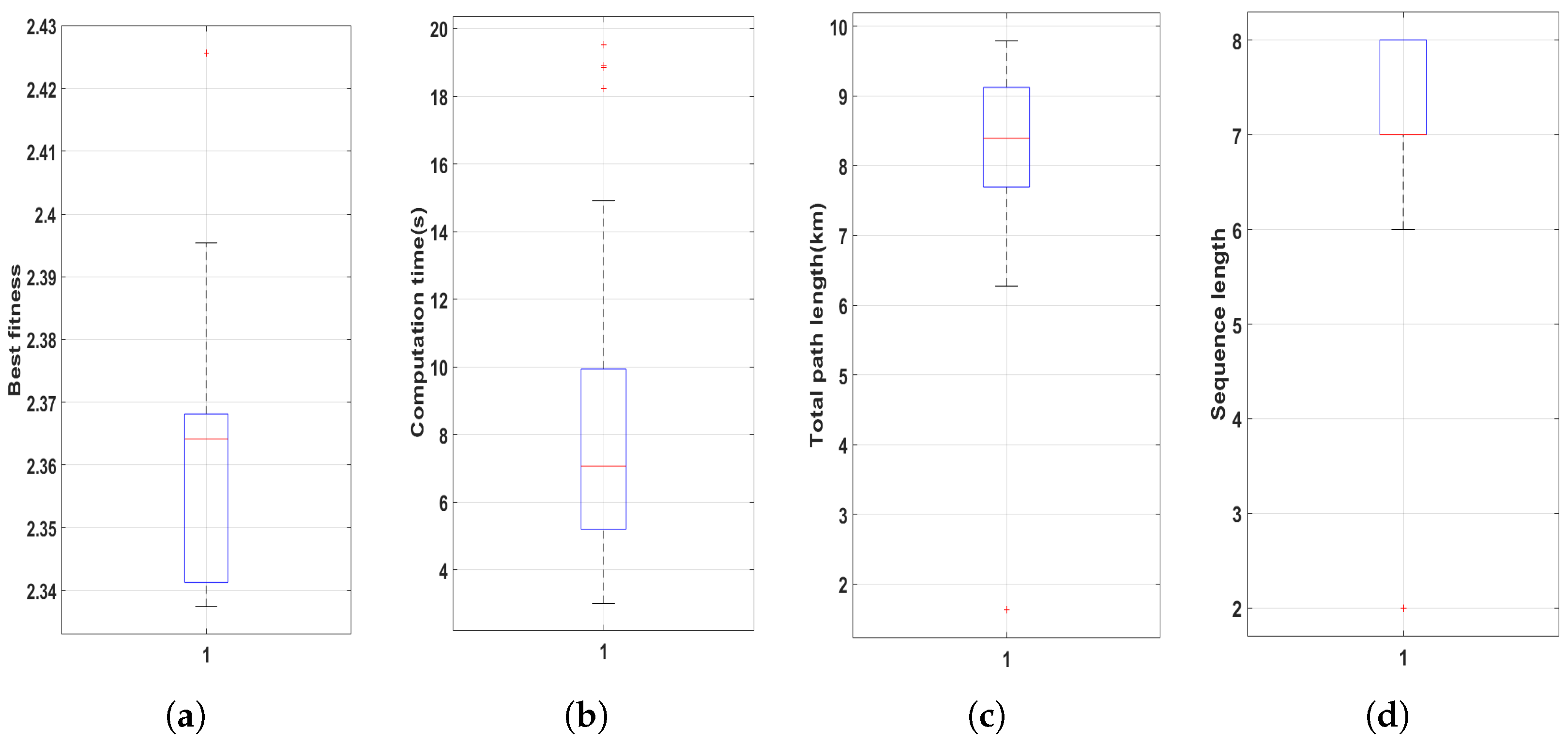
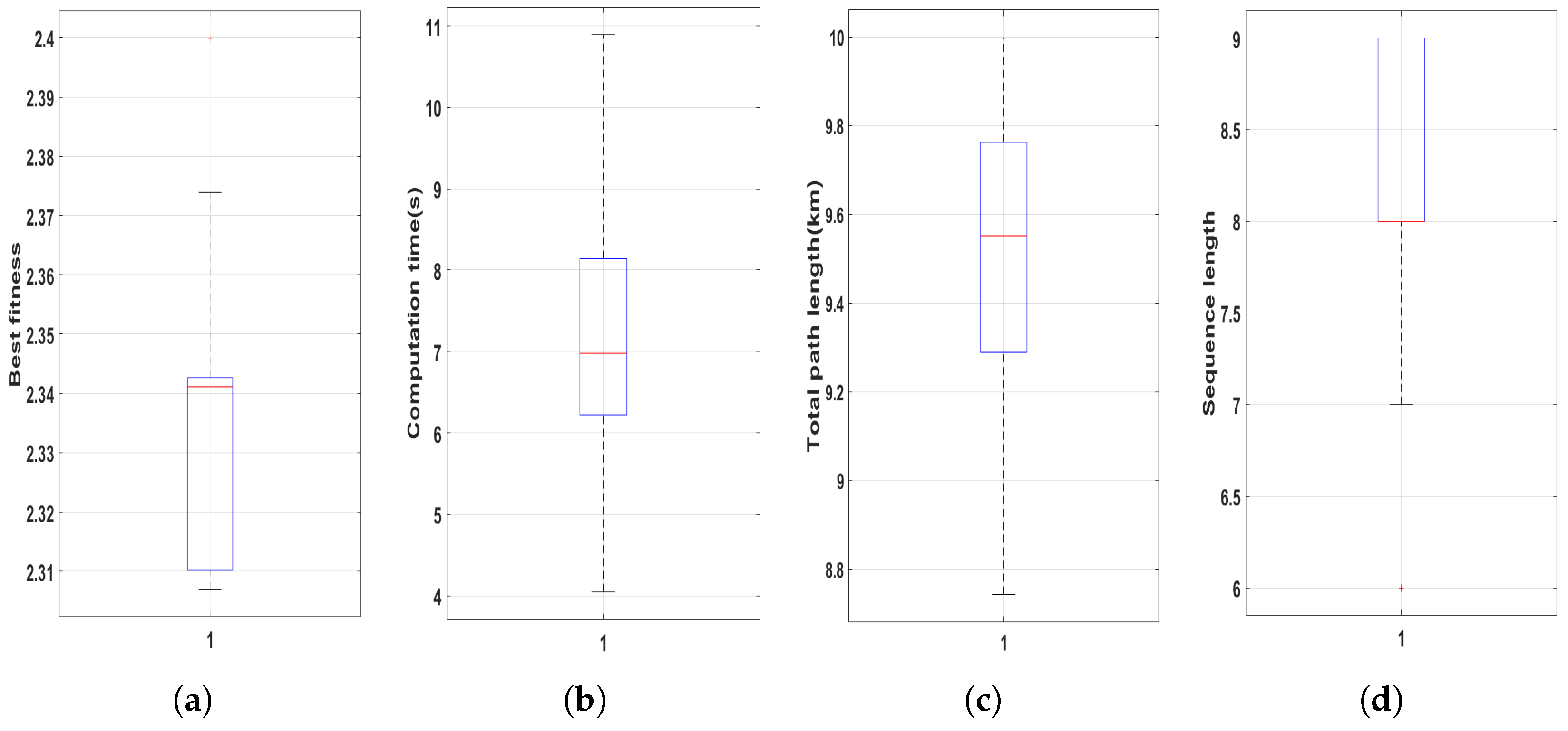
Figure 12 shows the box plot of statistic data for the scenario with 20 areas after 100 executions and

Table 7. Statistic data for 20 areas in DSSA simulation.

Performance Metrics	Q1	Median	Q3	Interquartile	Minimum	Maximum
Best fitness	2.3102	2.3411	2.3427	0.0325	2.3069	2.3739
Computation time (s)	6.222	6.9765	8.1437	1.9217	4.0457	10.892
Total distance (km)	9.2898	9.5517	9.7629	0.4731	8.7436	9.9982
Covered areas	8	8	9	1	7	9

lists the key metrics.

4.2. Comparison of GA and DSSA in Simulation

From the simulation results and data, it can be seen that both algorithms can optimize task-sequencing for an AUV with limited endurance, but the effect and performance of the two algorithms are still different. First of all, it can be seen from Table 3 and Table 6 that GA algorithm is slightly better than DSSA since the calculation time of GA algorithm is less than that of DSSA although the best fitness of both algorithms is similar. Secondly, in order to make a more accurate comparison, statistic data for the scenario with 20 areas after 100 episodes are analyzed. According to the key metrics of statistic data from Table 3 and Table 7, it can be seen that each quantile value of best fitness of DSSA is universally less than that of GA. And the total distance and covered areas of DSSA is more than these of GA. It can be shown that DSSA algorithm can make full use of endurance of AUV to obtain as many task benefits as possible compared with GA algorithm. Moreover, the optimization using GA algorithm presents some instability, for example, its interquartile value of computation time and total distance is larger. In addition, DSSA algorithm also has the advantage of fewer input parameters, which are mainly randomly generated except for the sizes of iteration and population.

In summary, DSSA has more advantages compared with GA. Therefore, in the following experiment, DSSA is selected and deployed in a physical AUV for verification.

4.3. Experiment Results

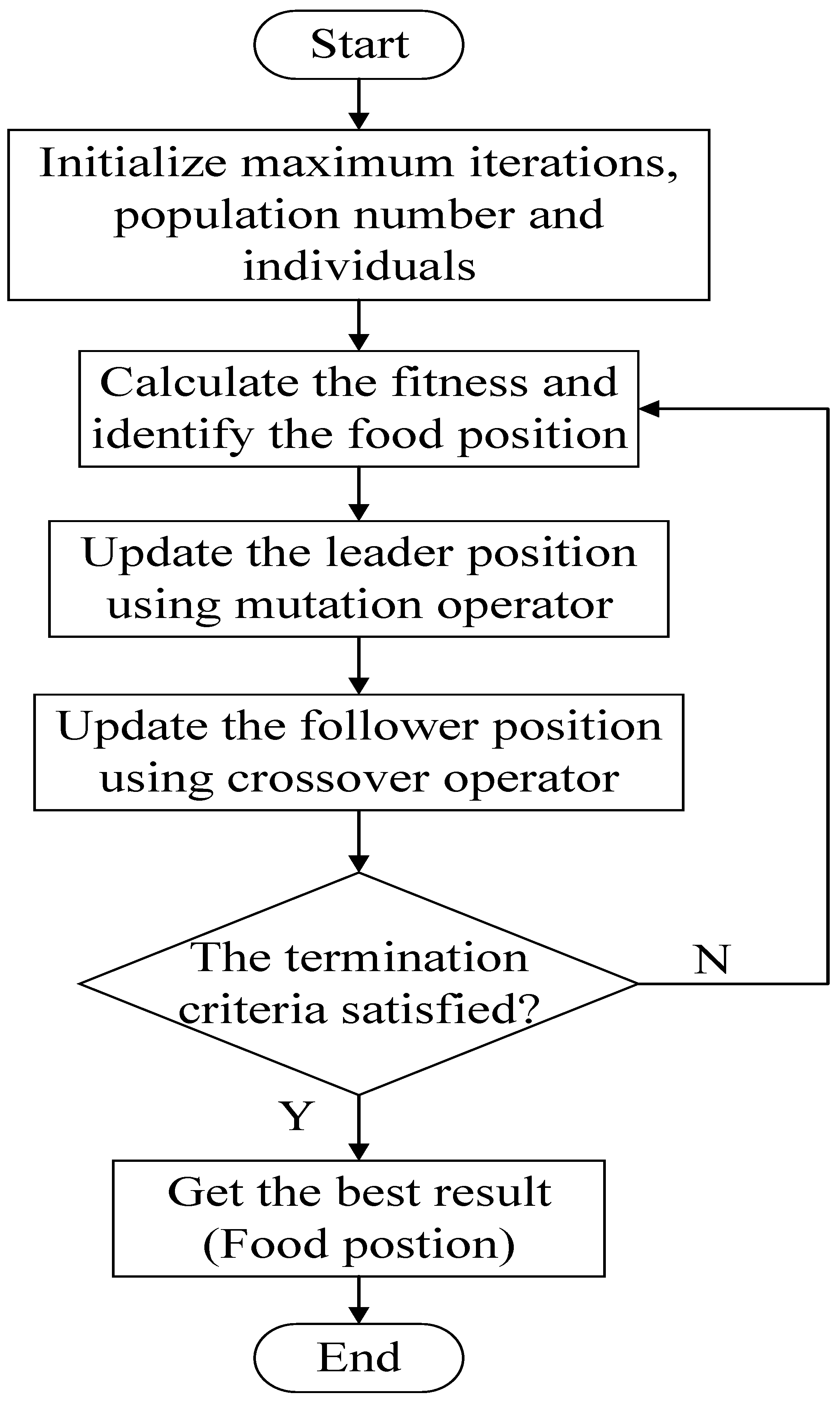
In order to verify the effect in actual equipment, DSSA was implemented and deployed in Sailfish AUV shown in Figure 13a. It is a kind of small underwater vehicle and developed in the Underwater Vehicle Laboratory of Ocean University of China. The diameter of the vehicle is 260 mm and weight is about 100 kg. Figure 13b presents the control architecture of Sailfish AUV and logical flow chart of DSSA implementation. Users can provision and send tasks from the deck monitoring interface to the control system in Sailfish AUV. The control system in Sailfish AUV consists of 4-layer function modules, i.e., task layer, behavior layer, motion layer and actuator. Optimization based on DSSA is mainly implemented at the task layer. As shown in Figure 13c, since the path planning function is in the behavior layer of Sailfish AUV, path planning requests need to be sent to the behavior layer to obtain path information before optimization. And considering the optimization process takes some time, a thread is set up to perform the optimization operation. After optimization, tasks are scheduled, decomposed into behaviors and sent to the behavior layer.

The experiments were carried out in a lake at Qingdao and were divided into two types. One type was that the total path length was less than the endurance of AUV, and the other was that the path length exceeded the endurance. In the experiments, the endurance of AUV was set to 5 km for the sake of simplicity, although the actual endurance of Sailfish AUV is much greater.

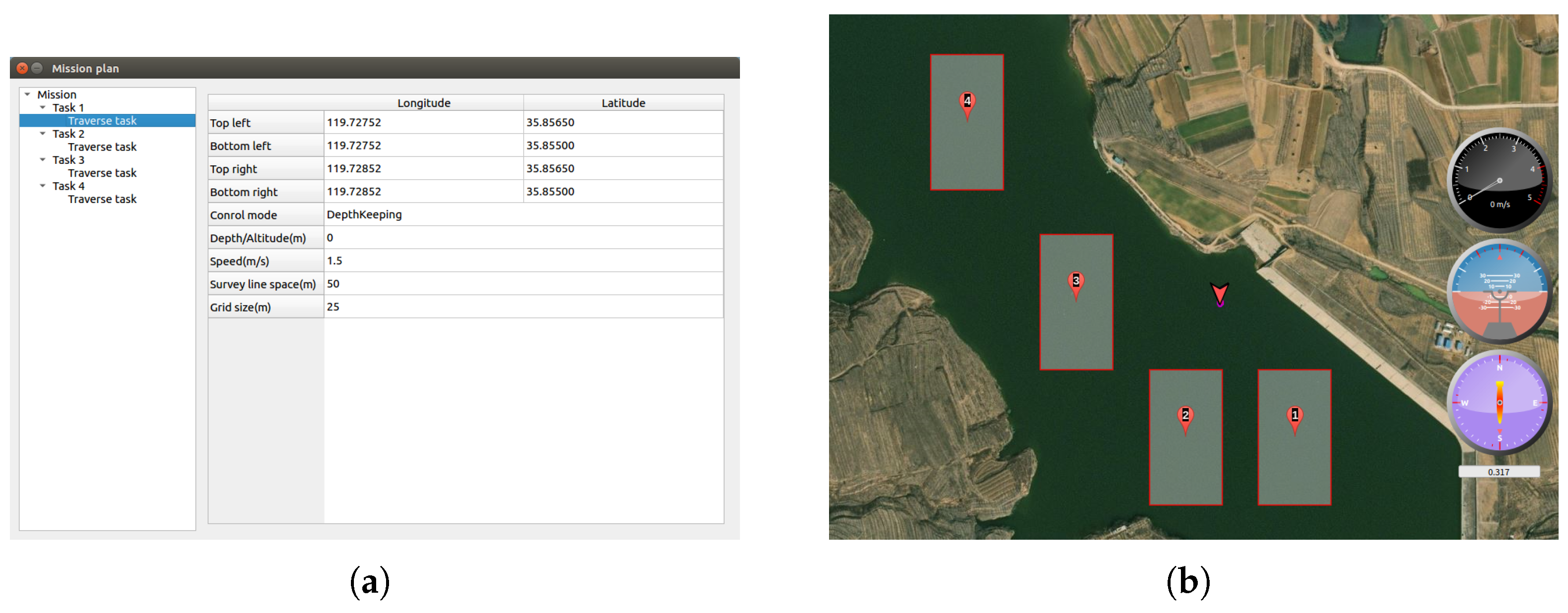
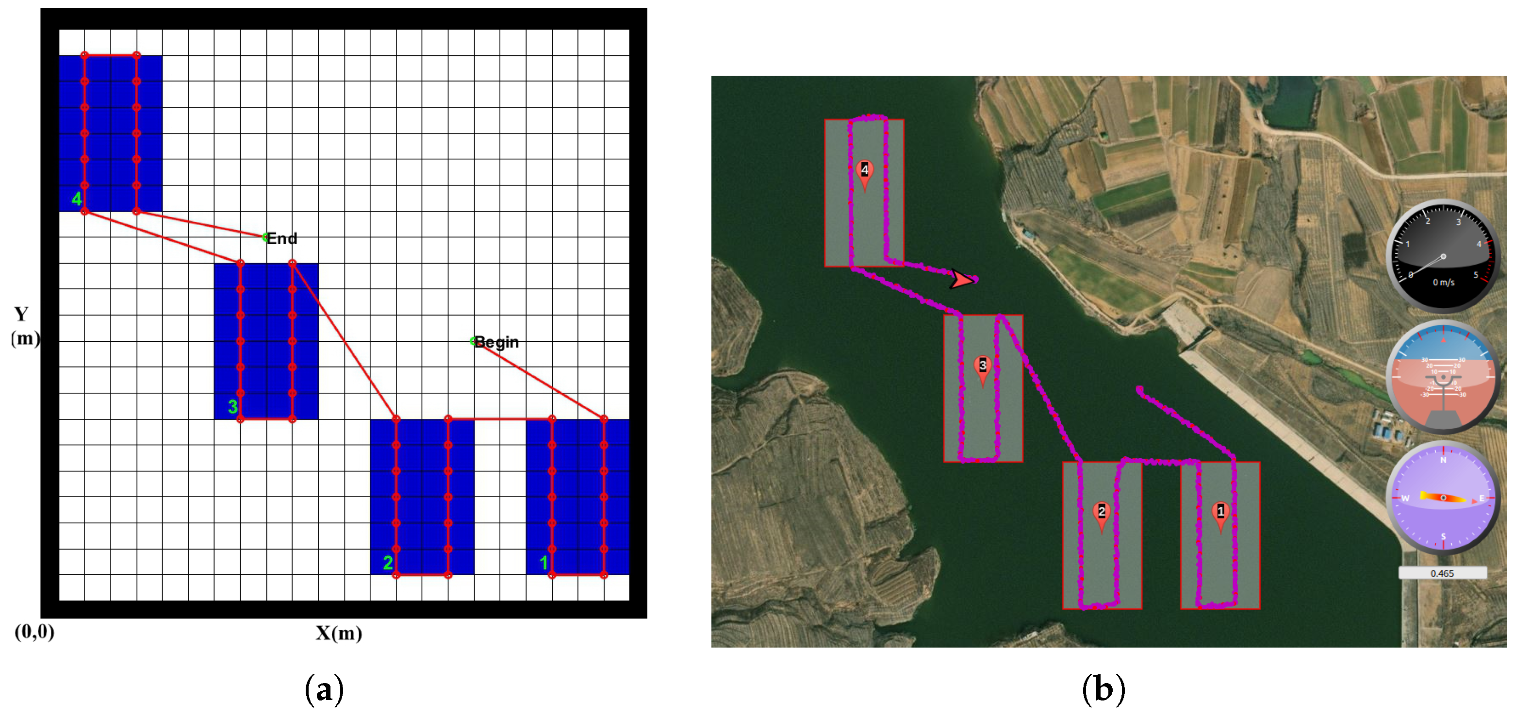
In the first experiment, there were 4 traverse tasks provisioned through the interface shown in Figure 14. In Figure 14a, each rectangular area is determined by the latitude and longitude values of four vertices, survey line space is 50 m, desired speed is 1.5 m/s and desired depth is 0m. In Figure 14b, the triangular arrow represents the start-point. The simulation result is shown in Figure 15a. In the diagram of the simulation, the width of a grid is 25 m. And the motion trajectory displayed in the deck monitoring interface is shown in Figure 15b. In the simulation, the optimized task sequence is 1-2-3-4 and the entry-point sequence is 3-3-3-1. In the experiment, the optimized task sequence is 1-2-3-4 and the entry-point sequence is 3-3-3-1. For this scenario, both results are optimal solutions. It can be seen that DSSA algorithm can work successfully and generate an optimization result in a physical AUV.

Like the first experiment, 4 traverse tasks were also provisioned in the second experiment, but the endurance was reduced to 2 km. The simulation result is shown in Figure 16a and the actual motion trajectory displayed in the deck monitoring interface is shown in Figure 16b. In the simulation, the optimized task sequence is 1-2-3 and the entry-point sequence is 3-3-3. In the experiment, the optimized task sequence is 1-2-3 and the entry-point sequence is 3-3-3. Due to the limit of endurance, three tasks were finally selected and executed after optimization.

5. Discussion

In this paper, DSSA algorithm is improved and applied to optimize the execution sequence of traverse tasks for an AUV. During the optimization, each individual chromosome consists of a task sequence and entry-point sequence, since both of them together determine the total path length. Besides that, the endurance of AUV is also taken into account, so that the total planning path length is not larger than the limited endurance. And by comparing the simulation results, DSSA has more advantages, such as fewer parameters, smaller best fitness, more covered areas and more stable performance. Therefore, DSSA is selected for deployment in a physical AUV and verified in the experiments. The experiment results show that DSSA is successfully applied to optimize the task sequence for AUV.

However, for the scenarios where the task execution time is uncertain or the shape of the task area is more complex, the method described in this paper needs to be improved further. Furthermore, in future study, re-optimization would be considered, since the endurance of AUV may change during the execution of tasks or the planned path may be different from the actual trajectory of AUV. Besides these, the optimization of task allocation and sequencing for multiple AUVs is also an important research direction.

References

1. Wynn, R.B.; Huvenne, V.A.I.; Bas, T.P.L.; Murton, B.J.; Hunt, J.E. Autonomous Underwater Vehicles (AUVs): Their past, present and future contributions to the advancement of marine geoscience. Mar. Geol. 2014, 352, 451–468. [Google Scholar] [CrossRef]
2. Sahoo, A.; Dwivedy, S.K.; Robi, P. Advancements in the field of autonomous underwater vehicle. Ocean Eng. 2019, 181, 145–160. [Google Scholar] [CrossRef]
3. Zhang, B.; Ji, D.; Liu, S.; Zhu, X.; Xu, W. Autonomous Underwater Vehicle navigation: A review. Ocean Eng. 2023, 273, 113861. [Google Scholar] [CrossRef]
4. Choset, H. Coverage of Known Spaces: The Boustrophedon Cellular Decomposition. Auton. Robot. 2000, 9, 247–253. [Google Scholar] [CrossRef]
5. Pyo, J.; Cho, H.; Joe, H.; Ura, T.; Yu, S.C. Development of hovering type AUV “Cyclops” and its performance evaluation using image mosaicing. Ocean Eng. 2015, 109, 517–530. [Google Scholar] [CrossRef]
6. Khan, M.T.R.; Ahmed, S.H.; Jembre, Y.Z.; Kim, D. An energy-efficient data collection protocol with AUV path planning in the Internet of Underwater Things. J. Netw. Comput. Appl. 2019, 135, 20–31. [Google Scholar] [CrossRef]
7. Mahmoud Zadeh, S.; Powers, D.M.W.; Sammut, K.; Yazdani, A.M. A novel versatile architecture for autonomous underwater vehicle’s motion planning and task assignment. Soft Comput. 2018, 22, 1687–1710. [Google Scholar] [CrossRef]
8. Alatartsev, S.; Stellmacher, S.; Ortmeier, F. Robotic Task Sequencing Problem: A Survey. J. Intell. Robot. Syst. 2015, 80, 279–298. [Google Scholar] [CrossRef]
9. Gavett, J.W.; Plyter, N.V. The Optimal Assignment of Facilities to Locations by Branch and Bound. Oper. Res. 1966, 14, 210–232. [Google Scholar] [CrossRef]
10. Padberg, M.; Rinaldi, G. Optimization of a 532-city symmetric traveling salesman problem by branch and cut. Oper. Res. Lett. 1987, 6, 1–7. [Google Scholar] [CrossRef]
11. Bellman, R. Dynamic programming treatment of the travelling salesman problem. J. Assoc. Comput. Mach. 1962, 9, 61–63. [Google Scholar] [CrossRef]
12. Younas, I.; Kamrani, F.; Bashir, M.; Schubert, J. Efficient genetic algorithms for optimal assignment of tasks to teams of agents. Neurocomputing 2018, 314, 409–428. [Google Scholar] [CrossRef]
13. Geng, N.; Chen, Z.; Nguyen, Q.A.; Gong, D. Particle swarm optimization algorithm for the optimization of rescue task allocation with uncertain time constraints. Complex Intell. Syst. 2021, 7, 873–890. [Google Scholar] [CrossRef]
14. Skinderowicz, R. Improving Ant Colony Optimization efficiency for solving large TSP instances. Appl. Soft Comput. 2022, 120, 108653. [Google Scholar] [CrossRef]
15. Mehmood, K.; Chaudhary, N.I.; Khan, Z.A.; Cheema, K.M.; Raja, M.A.Z. Design of quantum computing-based avain navigation optimization algorithm for parameter estimation of input nonlinear output error model with key term separation. Mod. Phys. Lett. A 2025, 40, 2550019. [Google Scholar] [CrossRef]
16. Mehmood, K.; Chaudhary, N.I.; Cheema, K.M.; Khan, Z.A.; Raja, M.A.Z.; Milyani, A.H.; Alsulami, A. Design of Nonlinear Marine Predator Heuristics for Hammerstein Autoregressive Exogenous System Identification with Key-Term Separation. Mathematics 2023, 11, 2512. [Google Scholar] [CrossRef]
17. Chen, P.; Liu, M.; Zhou, S. Discrete Salp Swarm Algorithm for symmetric traveling salesman problem. Math. Biosci. Eng. 2023, 20, 8856–8874. [Google Scholar] [CrossRef]
18. Panwar, K.; Deep, K. Discrete Salp Swarm Algorithm for Euclidean Travelling Salesman Problem. Appl. Intell. 2023, 53, 11420–11438. [Google Scholar] [CrossRef]
19. Katoch, S.; Chauhan, S.S.; Kumar, V. A review on genetic algorithm: Past, present, and future. Multimed. Tools Appl. 2021, 80, 8091–8126. [Google Scholar] [CrossRef]
20. Man, K.; Tang, K.; Kwong, S. Genetic algorithms: Concepts and applications [in engineering design]. IEEE Trans. Ind. Electron. 1996, 43, 519–534. [Google Scholar] [CrossRef]
21. Zacharia, P.; Aspragathos, N. Optimal robot task scheduling based on genetic algorithms. Robot. Comput.-Integr. Manuf. 2005, 21, 67–79. [Google Scholar] [CrossRef]
22. Zacharia, P.T.; Xidias, E.K.; Aspragathos, N.A. Task scheduling and motion planning for an industrial manipulator. Robot. Comput.-Integr. Manuf. 2013, 29, 449–462. [Google Scholar] [CrossRef]
23. Bu, W.; Liu, Z.; Tan, J. Industrial robot layout based on operation sequence optimisation. Int. J. Prod. Res. 2009, 47, 4125–4145. [Google Scholar] [CrossRef]
24. Huang, Y.; Gueta, L.B.; Chiba, R.; Arai, T.; Ueyama, T.; Ota, J. Selection of manipulator system for multiple-goal task by evaluating task completion time and cost with computational time constraints. Adv. Robot. 2013, 27, 233–245. [Google Scholar] [CrossRef]
25. Atyabi, A.; MahmoudZadeh, S.; Nefti-Meziani, S. Current advancements on autonomous mission planning and management systems: An AUV and UAV perspective. Annu. Rev. Control 2018, 46, 196–215. [Google Scholar] [CrossRef]
26. Zhang, H.; Ge, H.; Yang, J.; Tong, Y. Review of Vehicle Routing Problems: Models, Classification and Solving Algorithms. Arch. Comput. Methods Eng. 2022, 29, 195–221. [Google Scholar] [CrossRef]
27. Konstantakopoulos, G.D.; Gayialis, S.P.; Kechagias, E.P. Vehicle routing problem and related algorithms for logistics distribution: A literature review and classification. Oper. Res. 2022, 22, 2033–2062. [Google Scholar] [CrossRef]
28. Tasan, A.S.; Gen, M. A genetic algorithm based approach to vehicle routing problem with simultaneous pick-up and deliveries. Comput. Ind. Eng. 2012, 62, 755–761. [Google Scholar] [CrossRef]
29. Rabbouch, B.; Saâdaoui, F.; Mraihi, R. Efficient implementation of the genetic algorithm to solve rich vehicle routing problems. Oper. Res. 2021, 21, 1763–1791. [Google Scholar] [CrossRef]
30. Chen, G.; Shen, Y.; Zhang, Y.; Zhang, W.; Wang, D.; He, B. 2D multi-area coverage path planning using L-SHADE in simulated ocean survey. Appl. Soft Comput. 2021, 112, 107754. [Google Scholar] [CrossRef]
31. Chen, G.; Shen, Y.; Qu, N.; Wang, D.; He, B. Control architecture of autonomous underwater vehicle for coverage mission in irregular region. Ocean Eng. 2021, 236, 109407. [Google Scholar] [CrossRef]
32. MahmoudZadeh, S.; Powers, D.M.W.; Sammut, K.; Yazdani, A.M.; Atyabi, A. Hybrid Motion Planning Task Allocation Model for AUV’s Safe Maneuvering in a Realistic Ocean Environment. J. Intell. Robot. Syst. 2019, 94, 265–282. [Google Scholar] [CrossRef]
33. MahmoudZadeh, S.; Powers, D.M.W.; Yazdani, A.M. A Novel Efficient Task-Assign Route Planning Method for AUV Guidance in a Dynamic Cluttered Environment. In Proceedings of the 2016 IEEE Congress on Evolutionary Computation (CEC), Vancouver, BC, Canada, 24–29 July 2016; pp. 678–684. [Google Scholar]
34. MahmoudZadeh, S.; M.W Powers, D.; Sammut, K.; Atyabi, A.; Yazdani, A. A hierarchal planning framework for AUV mission management in a spatiotemporal varying ocean. Comput. Electr. Eng. 2018, 67, 741–760. [Google Scholar] [CrossRef]
35. Mahmoud Zadeh, S.; Powers, D.M.; Sammut, K. An autonomous reactive architecture for efficient AUV mission time management in realistic dynamic ocean environment. Robot. Auton. Syst. 2017, 87, 81–103. [Google Scholar] [CrossRef]
36. Mirjalili, S.; Gandomi, A.H.; Mirjalili, S.Z.; Saremi, S.; Faris, H.; Mirjalili, S.M. Salp Swarm Algorithm: A bio-inspired optimizer for engineering design problems. Adv. Eng. Softw. 2017, 114, 163–191. [Google Scholar] [CrossRef]
37. Abualigah, L.; Shehab, M.; Alshinwan, M.; Alabool, H. Salp swarm algorithm: A comprehensive survey. Neural Comput. Appl. 2020, 32, 11195–11215. [Google Scholar] [CrossRef]
38. Abadi, M.Q.H.; Rahmati, S.; Sharifi, A.; Ahmadi, M. HSSAGA: Designation and scheduling of nurses for taking care of COVID-19 patients using novel method of Hybrid Salp Swarm Algorithm and Genetic Algorithm. Appl. Soft Comput. 2021, 108, 107449. [Google Scholar] [CrossRef]
39. Firouz, N.; Masdari, M.; Sangar, A.B.; Majidzadeh, K. A novel controller placement algorithm based on network portioning concept and a hybrid discrete optimization algorithm for multi-controller software-defined networks. Clust. Comput. 2021, 24, 2511–2544. [Google Scholar] [CrossRef]
40. Barhoush, M.; Abed-alguni, B.H.; Al-qudah, N.E.A. Improved discrete salp swarm algorithm using exploration and exploitation techniques for feature selection in intrusion detection systems. J. Supercomput. 2023, 79, 21265–21309. [Google Scholar] [CrossRef]
41. Bye, R.T.; Gribbestad, M.; Chandra, R.; Osen, O.L. A Comparison of GA Crossover and Mutation Methods for the Traveling Salesman Problem. In Proceedings of the 2020 International Conference on Innovations in Computational Intelligence and Computer Vision, Jaipur, India, 17–19 January 2020; pp. 529–542. [Google Scholar]
42. Deep, K.; Adane, H.M. New Variations of Order Crossover for Travelling Salesman Problem. Int. J. Comb. Optim. Probl. Inform. 2011, 2, 2–13. [Google Scholar]
Figure 1. Graph representation of operating areas. The numbers from 1 to 4 represent four vertices of an area, i.e., four corners of an area. The letters from A to D indicate different areas.
Jmse 13 01111 g001
Figure 2. Four kinds of planned lawnmower paths from different entry-points for a task area. The numbers from 1 to 4 represent four corners of an area. (1) The planned path from entry-point in lower-left corner, (2) the planned path from entry-point in upper-left corner, (3) the planned path from entry-point in upper-right corner, (4) the planned path from entry-point in lower-right corner.
Jmse 13 01111 g002
Figure 3. Graph representation of planned path. The letters of A and B indicate the identity numbers of different areas.
Jmse 13 01111 g003
Figure 4. Graph representation of crossover for task area sequence. (1) represents Offspring-1 when the chromosome segment is from Parent-1, (2) indicates Offspring-2 when the chromosome segment is from Parent-2.
Jmse 13 01111 g004
Figure 5. Graph representation of crossover for entry point sequence. (1) represents Offspring-1 when the chromosome segment is from Parent-1; (2) indicates Offspring-2 when the chromosome segment is from Parent-2.
Jmse 13 01111 g005
Figure 6. Block diagram of the proposed DSSA algorithm.
Jmse 13 01111 g006
Figure 7. Diagram of evolution curve in GA simulation. (a) Scenario with 8 areas. (b) Scenario with 20 areas.
Jmse 13 01111 g007
Figure 8. Diagram of planning trajectory in GA simulation. (a) Scenario with 8 areas. (b) Scenario with 20 areas.
Jmse 13 01111 g008
Figure 9. Diagram of statistic data for scenario with 20 areas using GA algorithm. (a) Best fitness. (b) Computation time. (c) Total path length. (d) Sequence length after optimization.
Jmse 13 01111 g009
Figure 10. Diagram of evolution curve in DSSA simulation. (a) Scenario with 8 areas. (b) Scenario with 20 areas.
Jmse 13 01111 g010
Figure 11. Diagram of planning trajectory in DSSA simulation. (a) Scenario with 8 areas. (b) Scenario with 20 areas.
Jmse 13 01111 g011
Figure 12. Diagram of statistic data for scenario with 20 areas using DSSA algorithm. (a) Best fitness. (b) Computation time. (c) Total path length. (d) Sequence length after optimization.
Jmse 13 01111 g012
Figure 13. Diagram of Sailfish AUV and algorithm implementation. (a) Sailfish AUV. (b) Control architecture in AUV. (c) Logical flow chart of algorithm implementation.
Jmse 13 01111 g013
Figure 14. Diagram of task information in first experiment. (a) Task information through user interface. (b) Task display in the map.
Jmse 13 01111 g014
Figure 15. Diagram of trajectory. (a) Planning trajectory in the simulation. (b) Actual trajectory in the experiment.
Jmse 13 01111 g015
Figure 16. Diagram of trajectory limited by endurance. (a) Planning trajectory in the simulation. (b) Actual trajectory in the experiment.
Jmse 13 01111 g016