Empirical Geomorphic Approach to Complement Morphodynamic Modeling on Embayed Beaches

Abstract

In a coastal engineering project, hydrodynamic models are used to study wave transformations and impacts on structures, while morphodynamic models are applied to calculate the response and evolution of sedimentary beaches. Conventionally, laboratory experiments and numerical modeling have been called to investigate beach changes, particularly those resulting in the formation of an embayed beach. The former is undertaken in a wave basin, necessitating a huge outdoor facility to fit a project with large dimensions, numerous instrumentations, and manpower, while the latter is performed by powerful numerical models on a desktop, requiring only the advent of computing power and professional skills. Conventionally, both approaches have successfully achieved the expected outcome, though differing in cost and time frame. On the contrary, an efficient empirical geomorphic model for headland-bay beaches has been available since 1989 for assessing the planform stability of a crenulated beach in static equilibrium. The model can readily produce a graphic display of the static bay shape aided by a supporting software within a shorter time frame (in a couple of minutes), instead of in hours or days in laboratory tests and numerical modeling. Several practical examples drawn by the software MeePaSoL for the empirical model are presented to complement the results of a morphodynamic model in a wave basin, as well as to guide the modeler to terminate the programming when equilibrium is reached. We believe this alternative approach could be helpful for the experimentalists and numerical modelers on large engineering projects associated with shoreline beach evolution and shore protection, especially for time-saving and reducing manpower and cost.

1. Introduction

Interaction between hydrodynamic and morphodynamic processes is a common phenomenon in the ocean. Where coastal projects for harbors and shore protection are required, their interaction could result in shoreline change, producing an embayed beach at downdrift or in the lee of the structures. Nowadays, the applications of coastal engineering knowledge are wide ranging, with more focus on coastal sedimentation problems. This situation occurs, firstly, from wave propagation and its impact on offshore structures and harbor breakwaters, which are calculated using wave hydrodynamic models, and then the evolution of beaches is estimated by morphodynamic models. Although similar results can be obtained from a scaled laboratory experiment, a numerical model is now a more favorable choice, since sophisticated software with powerful processors in computers can display colored graphic outputs after complicated numerical computations.

Comparing the two conventional approaches, laboratory experiments and numerical models, the former is undertaken in a wave basin, necessitating a huge outdoor facility to fit a project with large dimensions, numerous instrumentations, and manpower; while the latter is performed by powerful numerical models on a desktop, requiring only the advent of computing power and professional skills. Both approaches have successfully achieved the anticipated outcome, though differing in cost and time frame. Both approaches also choose a specific set of statistical wave parameters (significant H_1/3 and T_1/3, or spectral peak period T_p from wave records) to represent the random wave field in the hydrodynamic models and to operate continually within a limited duration of the entire laboratory tests and numerical modeling.

Intuitively, the result of the morphodynamic response, particularly in bay beach evolution, may differ from that produced by nature in field conditions, due to differences in the fluctuations in wave complexities (magnitudes and obliquity), water levels, and seabed conditions (sediment grain sizes, sorting, and thickness). Therefore, it is fair to state that the morphodynamic results on bay beach processes in the laboratory and on a desktop may not be “perfect”, though “correct” scientifically and mathematically, compared to the outcome that nature has displayed in field conditions. Therefore, it would be helpful if a different approach can be produced to complement the results of laboratory tests and morphodynamic models.

Overall, three methods have been undertaken to investigate coastal evolution or shoreline change. These include (1) laboratory tests, (2) prototype experiments, and (3) numerical modeling. Among them, each has its own requirements of manpower, time, instrumentations, and costs. For example, wave hydrodynamic models have played significant roles in modeling short-term (e.g., seasonal to multiannual) morphological change and long-term (e.g., decadal to centennial) processes (such as natural and anthropogenic effects, longshore and cross-shore transport, and climatic variations) [1]. Many different coastal evolution models have also existed to simulate individual behavior of certain forcings, processes, and scales, with necessary assumptions. Although a computer may yield spurious outputs, a numerical modeling is more cost-effective than physical modeling, if the problem in coastal processes is thoroughly understood before model formulation. Moreover, although computational error cannot be avoided in numerical models, because simplified approximations are made to represent the intricate relationship in the physics-based process, they can provide useful results and aid in understanding and predicting shoreline evolution.

Several well-known physics-based 2-D and 3-D models have been developed by leading research institutes and universities in the world and are available for use, which have coupled wave hydrodynamics and sediment transport to simulate morphodynamic processes [2]. These include Mike21 [3], Delft3D [4], GENESIS [5,6], SBEACH [7,8], XBeach [9], and ROMS [10], and others. These models solve the conservation of mass and momentum of fluid and sediment and calculate coastal evolution. Vitousek et al. [1] have commented that “Physics-based models have becoming increasingly capable of simulating small-scale, short-term beach and dune erosion due to storm events on timescales of days and weeks”. But “physics-based simulations of large-scale (e.g., 100 m to 100 km length scale) or long-term (e.g., annual to decadal timescale) shoreline change (such as beach recovery) is often prohibitively expensive in computation cost and do not necessarily provide improved skill over simplified models”. Hence, the process-based models, (e.g., equilibrium beach profile models [11], equilibrium shoreline models [12,13,14,15,16,17], and one-line models [18,19,20,21]) are straightforward and computationally efficient [1]. For simulations of the morphodynamic process, different longshore sediment transport (LST) equations are used [22,23,24,25], particularly the “CERC equation” [23] and “Kamphuis equations” [24,25], which may differ in terms of the estimated quantities.

The total length of the Earth’s coastline is estimated to be around 444,000 km, of which about 50% is hilly or rocky, implying that beaches could form between their extremities [26,27]. This large percentage exhibits an abundance of natural headland-bay beaches (HBBs), in addition to those produced unintentionally by coastal engineers. HBBs have occurred at:

(1)

Downdrift of a shore-normal groin with moderate protrusion into the sea under oblique swell;

(2)

Downdrift or between a complex groin receiving normal incident waves;

(3)

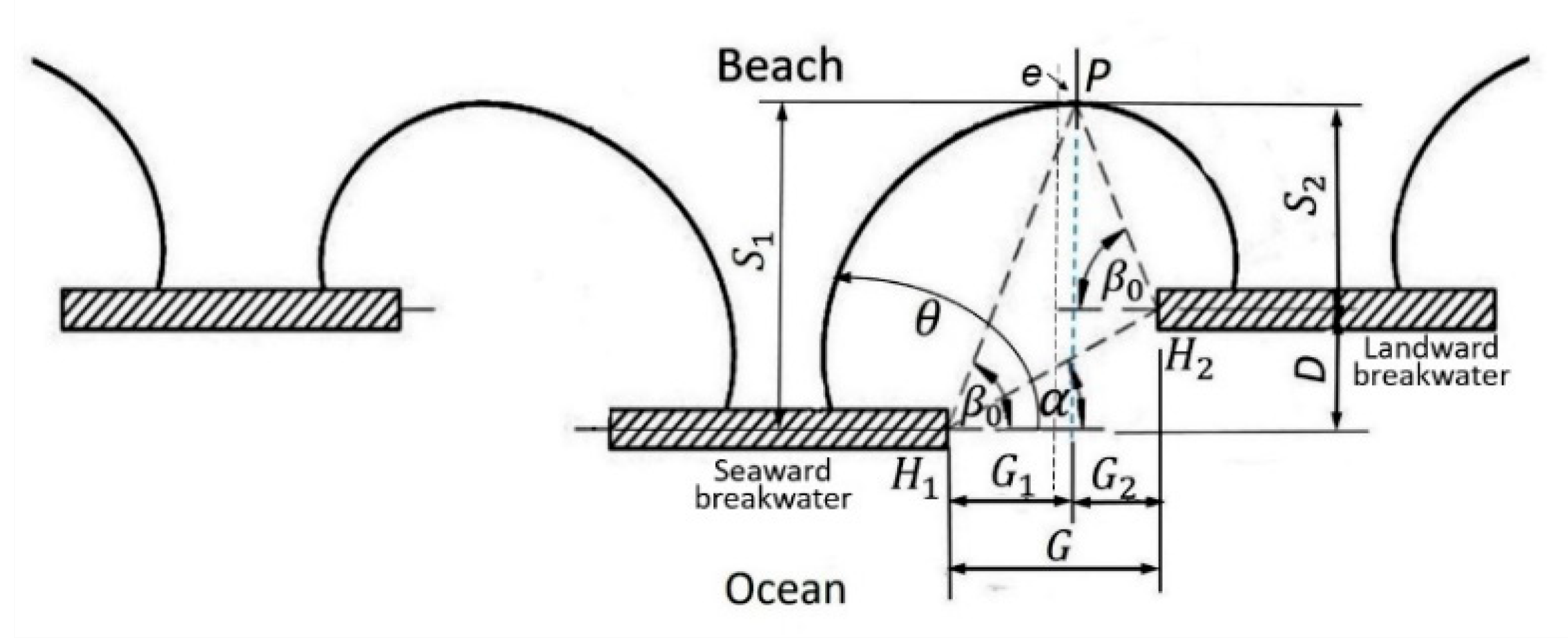
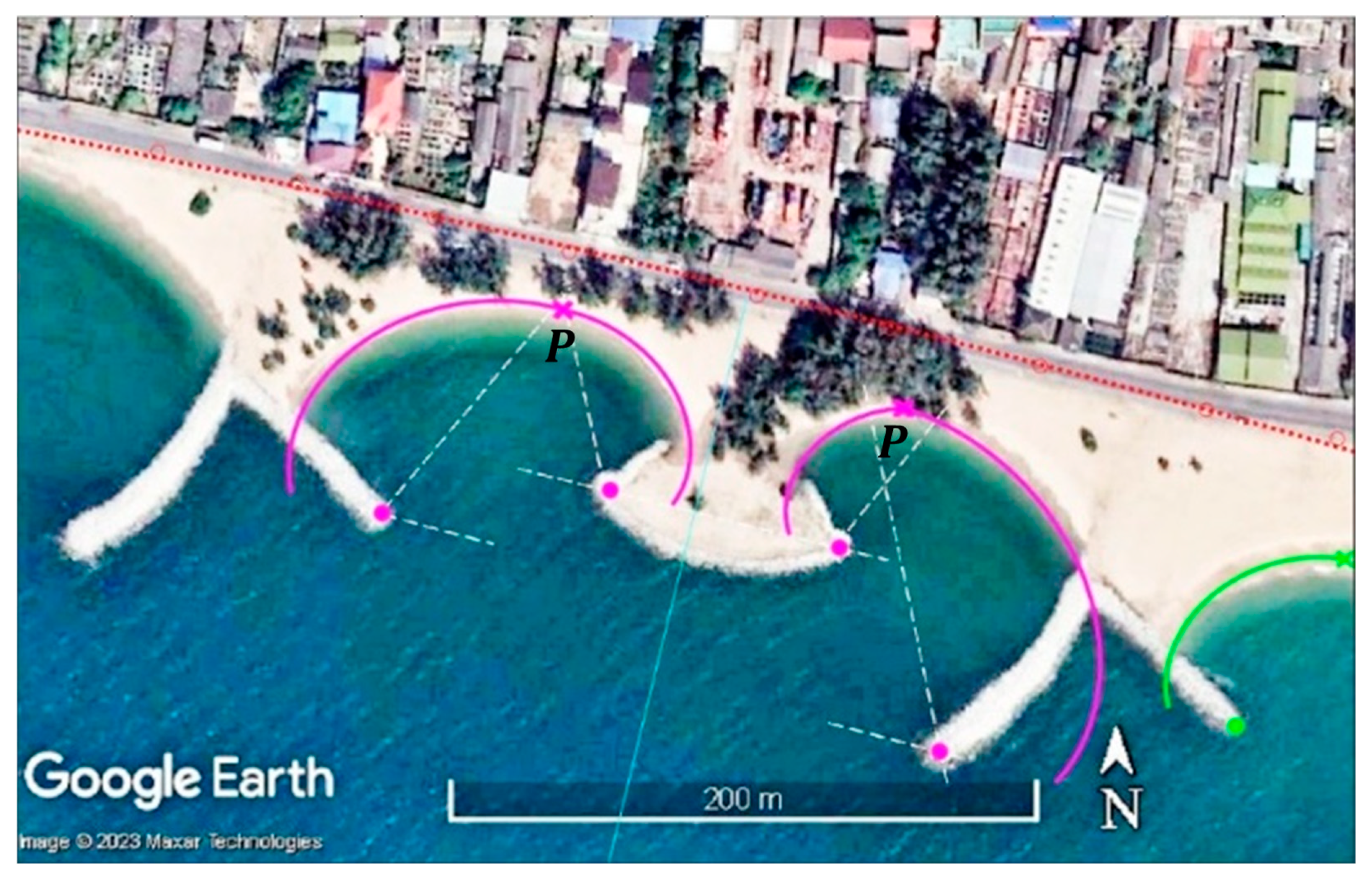
Between detached breakwaters; and

(4)

Downdrift of the out breakwater for a harbor, port, or marina (for yacht).

The curved planforms, whether single or double curvature, produced by combined wave diffraction and refraction, have been successfully tested in the laboratory [28,29] and designed for recreation [30]. These specific features, produced by nature or humans, are good examples for coastal scientists, engineers, and managers to study to benefit their work on coastal projects.

On modeling shoreline evolution, it is worth noting that only limited reports have been published using morphodynamic models on sandy beaches with significant planform curvature [31] or inclusion of LST with wave diffraction [32], not to mention that those with double symmetrical curvature [33]. Perhaps it is even rare to find publication of numerical modeling on asymmetrical double curvature with much smaller embayments within a large outer embayment [34], such as that constructed at Pedregalejo, 4.5 km east of Málaga in southern Spain (Figure 1). Should this be manually tested in a laboratory or performed by a hydrodynamic and morphodynamic model, it would become strenuous and time-consuming to assess the resulting planform stability, especially for the accuracy of the six small asymmetrical bay shapes in close proximity to the three round-headed groins.

Nowadays, verification of beach stability could be readily carried out by applying an empirical model developed from geomorphic knowledge [35], aided by a suitable software [36,37]. The parabolic model uses a “parabolic bay shape equation” (PBSE; Hsu and Evans [35]), which is derived from a mix of 27 bay beach data from laboratory test results and prototype bays believed to be in stable condition. The PBSE is a second-order polynomial equation in polar coordinates. It has been proven reliable for assessing the stability of the shoreline planform of a crenulated beach in static equilibrium conditions [30]. Here, the word “static” does not infer a stable state in geological time; instead, it is for at least stable conditions seasonally with prevailing waves from a particular predominant direction. Although MEPBAY 3.0 [36] and MeePaSoL [37] were developed to facilitate the application of the parabolic model [35], they differ in the background approach of defining the downdrift control point (DCP). The former subjectively chooses a point on the near straight downdrift, taking it to be the “correct” control point, where the shoreline tangent is perpendicular to the predominant wave orthogonal. The classification of planform stability (static, dynamic, and unstable) has been defined [36]. However, this approach renders uncertainty in locating the DCP [38,39]. On the contrary, the latter locates the DCP by digitizing a stretch of downdrift shoreline that include the possible DCP location, from which a circle or curve is drawn by fitting the digitized data, and the predominant wave direction is determined and displayed on the beach image. Together with computer software, this empirical model can readily produce a graphic result of the static shoreline planform within a much shorter time frame (often in a couple of minutes), rather in hours or days in laboratory tests and with numerical modeling.

The objective of this paper is to offer an empirical geomorphic model with software that can produce a reliable graphic result for an embayed beach in static equilibrium, and apply it to assist workers engaging in morphodynamic studies for determining whether their calculated beach has also reached static conditions. This approach applies the now well-used parabolic bay shape equation (i.e., parabolic model [35]) for HBBs in static equilibrium with the support of the software MeePaSoL [37]. This combination is helpful not only for experimentalists who wish to observe beach changes in a laboratory basin with shore protection structures on a sandy beach, but also for numerical modelers who want to verify the results of a feasible option from a morphodynamic model, helping both to determine when the equilibrium stage is reached. This concept is based on the experience of the authors and others who have collectively researched HBBs over the 40 years since 1985 [40].

Following a brief introduction (Section 1) that outlines the hydrodynamic and morphodynamic models available and the need for an alternative to complement the results of morphodynamic modeling, the background knowledge of the parabolic model and MeePaSoL is described (Section 2). Examples of geomorphic results for embayed shoreline planforms (e.g., behind detached breakwaters and others) are demonstrated (Section 3), including the work of Tsai et al. [41] and Chen [42], who applied a numerical model available in the public domain (e.g., XBeach), along with many practical cases taken from prototype conditions. Discussions are provided (Section 4) on the advantages and issues associated with the application of the empirical model, as well as a case study of the construction history to produce the final beach planform in Greece. Finally, concluding remarks are made (Section 5), stating that the simple empirical method presented in this paper could benefit the coastal engineering community (researchers, practitioners, managers, and geographers) at large for modeling and planning shore protection and beach restoration projects using a headland-bay beach system.

2. Methods and Tools

2.1. Parabolic Model

Notwithstanding a large family of HBBs in various sizes, shapes, geological settings, and hydrodynamic conditions, coastal geologists and engineers have attempted to mathematically define their planforms since 1944. Of the equations available (logarithmic [43], parabolic [35], and hyperbolic–tangent [44,45]), only the parabolic model has remained the most used tool for planning [30,46], due to it:

(1)

Being derived from a mixed set of model and prototype bays believed to be in static equilibrium;

(2)

setting the origin of the coordinate system at the wave diffraction point (i.e., the tip of a headland);

(3)

recognizing the orthogonality between the predominant wave direction to the tangent at the downdrift control point; and

(4)

classifying beach stability based on the existing planform in relation to an ideal static equilibrium planform defined by the parabolic model.

It is worth noting, however, that the term “static equilibrium” does not denote a stable state in a geological time frame, nor in yearly terms, but rather seasonally, because nature has continually strived to produce an equilibrium state for every beach between the external wave forcings (wave conditions and direction) and the resulting beach profile and shoreline planform. This remark is derived from the phenomenon that “Beaches tend to build up transverse to the direction of approach of the most important beach constructing waves”, as concluded by Lewis [47] and consequently confirmed by Jennings [48] and Davies [49], based on the long-term results of their observations of stable bay beaches in Australia.

By defining a prevailing wave direction to an HBB in static equilibrium, the parabolic model was developed [35] from a mixed data set of 27 shoreline planforms in polar coordinates (13 laboratory tests and 14 prototype cases believed to be in static equilibrium). It defines the static planform (SEP) in single curvature (Figure 2), at which point Q (θ, R) on the curved shoreline can be calculated by:

$$R=R_{\beta }\left[C_0+C_1\left(\mathsf{\beta }/\mathsf{\theta }\right)+C_2{\left(\mathsf{\beta }/\mathsf{\theta }\right)}^2\right] \mathrm{f}\mathrm{o}\mathrm{r} \theta \ge \beta$$

(1)

$$R={\displaystyle \frac{a}{\sin \theta }} \mathrm{f}\mathrm{o}\mathrm{r} \theta <\beta$$

(2)

In Equation (1), R denotes the radial distance from an updrift control point (i.e., wave diffraction point or breakwater tip) to point Q, and $\theta$ is the angle between the wave crest baseline (i.e., wave front) at the tip and the radius to point Q. Parameter a (the indentation) is the vertical distance between the wave front and the tangent at the downdrift control point P, which runs parallel to the former. Angle $\beta$ represents the reference wave obliquity between the wave front and the control line $R_{\mathsf{\beta }}$, which connects the tip to point P (the downdrift control point, DCP). The three C coefficients ($C_0$, $C_1$, and $C_2$) in Equation (1) are the constants for a second-order polynomial, whose values are a function of $\beta$ obtained by fitting each set of 27 $C_i$ (i = 0, 1, 2) coefficients for $\beta$ values ranging from 22.5° to 72° (Figure 3). These C coefficients were later modified slightly applying the boundary condition at P (Figure 2), where $\theta$ = $\beta$ and where the sum of $C_i$ (i = 0, 1, 2) equals unity (Tan and Chiew [50] and Uda et al. [51]).

Equation (1) was derived for an HBB with single curvature, such as for the definition sketch (Figure 2). To apply it to a static bay beach in symmetrical double curvature under normal incident waves, such as that between two consecutive detached breakwaters (Figure 4), the common DCP is located at the mid-point on the curved planform, from which each half of the static bay shape can be sketched. Mathematically, the location can be found from the condition of $\mathsf{\partial }\left(R\mathrm{s}\mathrm{i}\mathrm{n}\theta \right)/\mathsf{\partial }\theta$ = 0 at the common DCP, $\theta$ = β for $C_0+C_1+C_2$ = 1, rendering the basic wave angle β₀ = $\theta$ = 65.75° measured from the wave crest line at a wave diffraction point [34].

For asymmetrical double curvature (Figure 5), the basic wave angle β₀ = 65.75° is measured from the wave crest line at each wave diffraction tip (e.g., updrift control point $H_1$ and $H_2$ in Figure 5). To design an HBB, a straight line (dashed line in Figure 5) is then projected shoreward to find an intersection to be called “the common DCP” (e.g., point P in Figure 5), which serves the downdrift DCP for sketching each half of the whole bay with the software MeePaSoL (Section 2.2). To verify the stability of an existing HBB, however, this common DCP could be moved from seaward to shoreward from the intersection along the direction (alignment) of the wave orthogonal displayed on the screen.

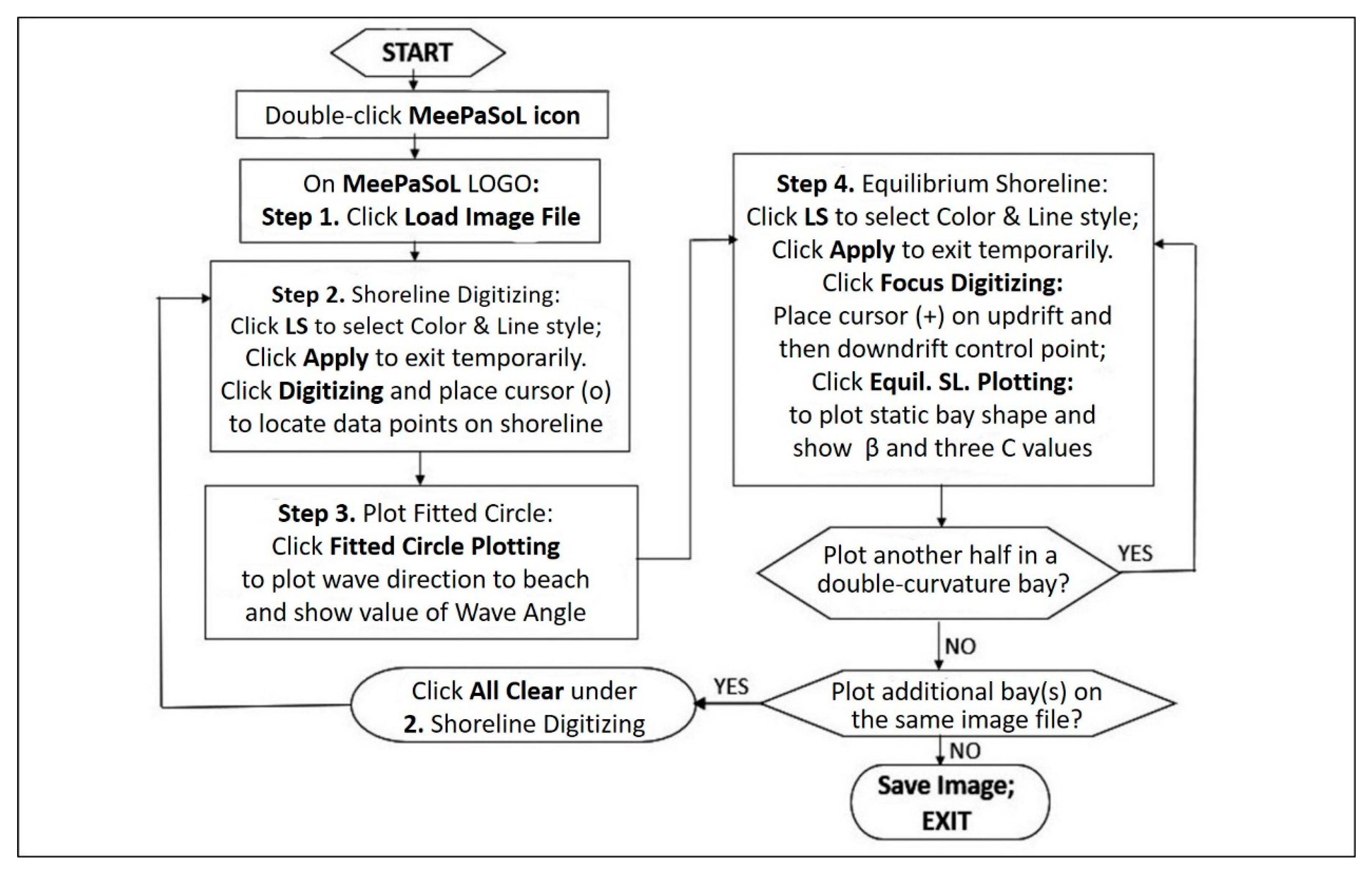
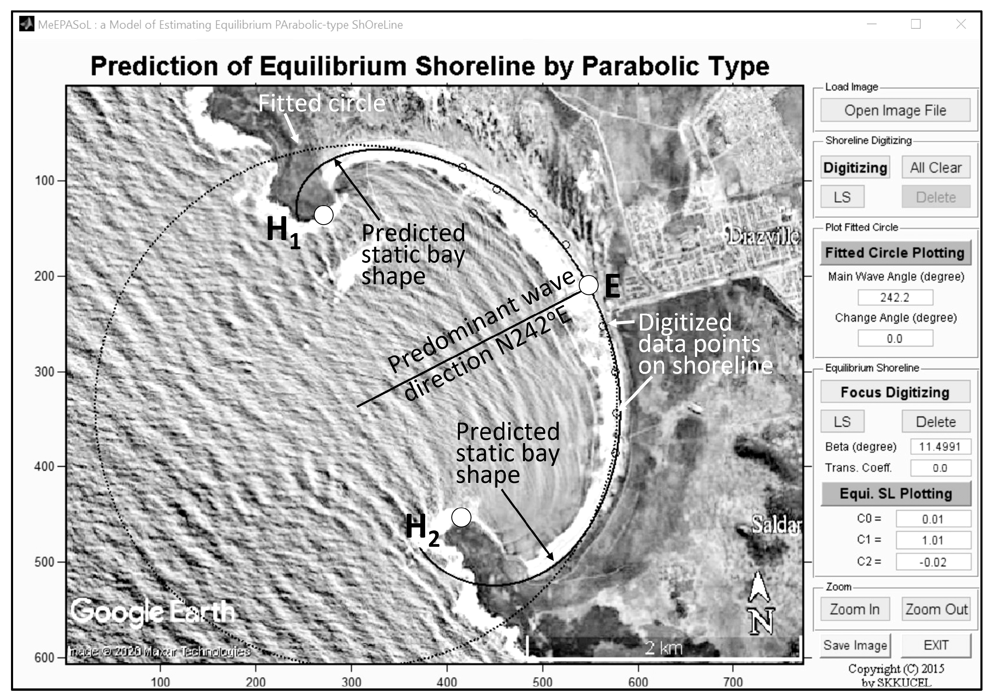
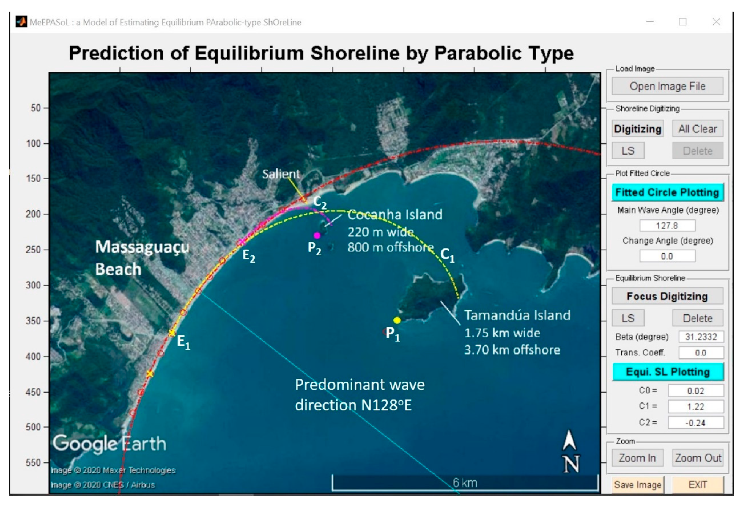
2.2. Software MEPBAY and MeePaSoL

The software MEPBAY, which stands for “Model for Equilibrium Planform of BAY beaches”, was developed as an educational tool to aid students in learning parabolic model application on several beaches in Brazil (Klein et al. [36]). Consequently, this software tool has since become a morphological model for evaluating beach stability and predicting shoreline changes caused by installing coastal structures. Examples of applying MEPBAY to three bay beaches in Brazil were given to demonstrate the beach stability, with each classified as being in “static equilibrium”, “dynamic equilibrium”, or “natural reshaping or unstable”. However, due to the issue of uncertainty of locating the DCP [38,39], this software is not used to present the examples in the paper.

The software MeePaSoL, which stands for “Model for Estimating Equilibrium PArabolic-type ShOreLines”, is a MATLAB-GUI-based programming package developed at Sungkyunkwan University’s campus in Suwon, Korea (Lee [52]; Lim et al. [37]; see “Software availability for MeePaSoL” below in Section 5). It applies the parabolic bay shape equation, Equation (1), and produces a screen display for an ideal static bay shape to be visually compared with an existing beach planform. The graphic result is then to be used for assessing or predicting the planform stability of an HBB. The software MeePaSoL can be used at different operational levels in the pre-design and planning phases of coastal engineering projects.

The user can smoothly operate the software following a set of stepwise procedures (flowchart in Figure 6) shown in the right-hand-side panel of the operation logo on screen (Figure 7). For example, after digitizing a set of shoreline points (data in small “o” dots) centered approximately around the potential downdrift stretch of the downloaded beach image, the program marks the predominant wave direction, as well as the radius of the fitted shoreline (circle, semi-circle, or nearly straight line), the length of which depends on the overall distribution of the digitized data. An ideal SEP is then drawn following the selection of a pair of updrift and downdrift control points (in that order). For example, updrift control point H₁ in Figure 7 with the common DCP at E (“o”) renders static curve H₁-E, while point H₂ with E gives static curve H₂-E, to complete the whole SEP for the double-curvature planform at Diazville (33°01′04″ S, 17°53′11″ E) in South Africa.

3. Results and Examples

For a 3-D morphodynamic modeling on a beach with significant planform curvature, such as an embayment, oblique wave transformation may induce asymmetrical current circulation, causing complex sediment movement patterns within the model domain, especially in the vicinity of coastal structures. Therefore, it may become difficult to determine whether the output of beach evolution has reached a stable condition (or in equilibrium) at a particular runtime, hence calling for a reliable empirical geomorphic model to help decide whether to continue or stop the modeling. Two cases for applying the parabolic model to complement the output of the shoreline planform from a combined hydrodynamic–morphodynamic model are first demonstrated in the following sub-sections, with additional examples for a complex planform and beach downdrift of a harbor extension for engineering applications to complement the work of numerical models.

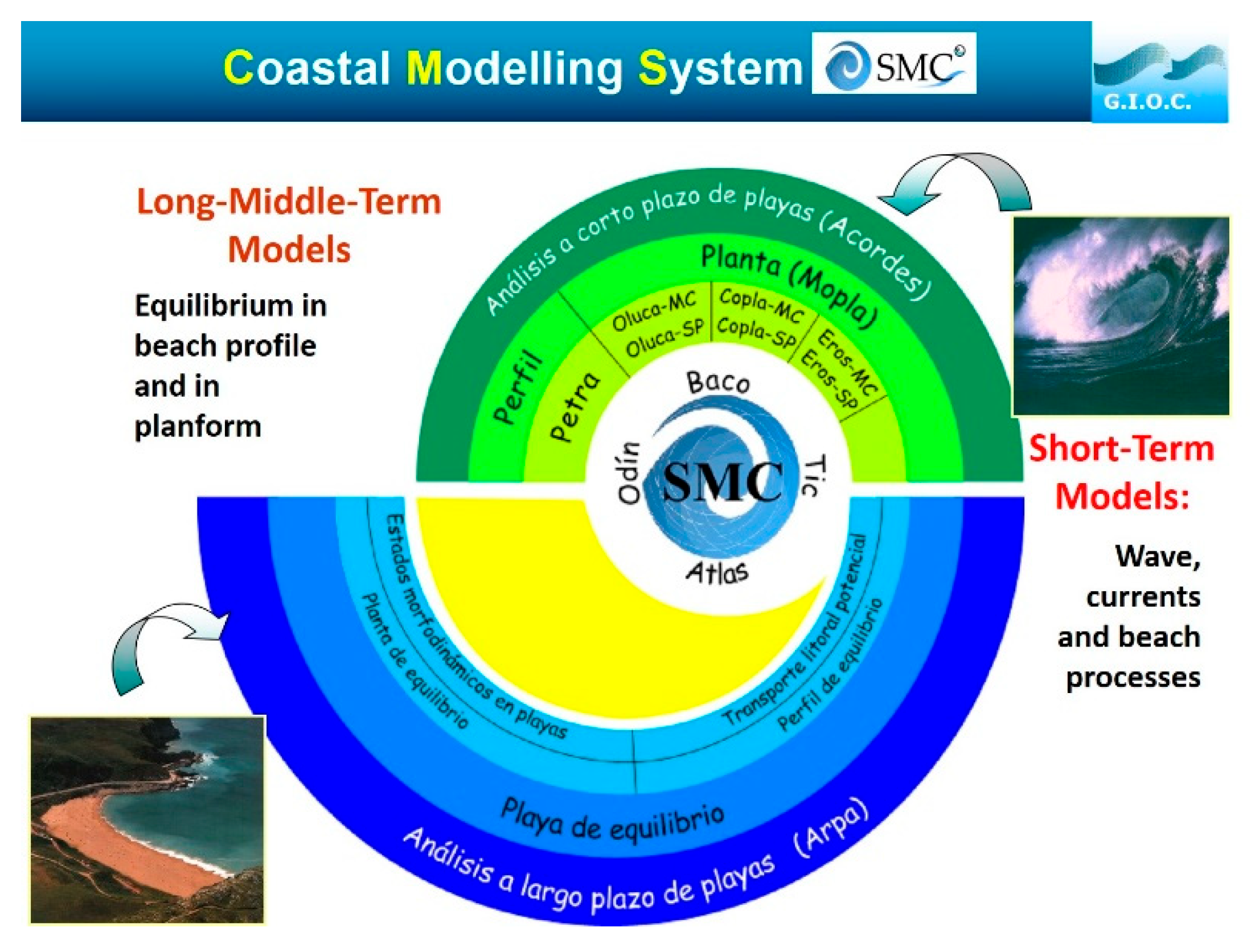
3.1. Parabolic Model as an Integral Component in SMC

Another case of applying the parabolic model to evaluate coastal projects and design a bay beach in static equilibrium can be found in the SMC (Coastal Modeling System) produced at IH-Cantabria, University of Cantabria, Spain. The SMC was developed (1) to establish a methodology to design, execute, and follow up with coastal projects; (2) to prevent coastal erosion and to estimate flood risk of low Spanish littoral zones; (3) to better know the dynamics and evolution of the Spanish coastline; and (4) to compile the experience in the coastal engineering field (González & Medina [53]; González et al. [54]). This system contains three major components: (1) science-based documents, (2) engineering-based documents, and (3) numerical tools.

In Figure 8, the thematic documents as the integrated modules in the SMC contain the following:

(1)

Pre-processing includes Baco (bathymetric data), Atlas (flood-level data), and Odin (wave and dynamic characteristics and model, and morphodynamic states);

(2)

Short-term analysis includes Mopla (beach morphodynamic evolution) and Petra (beach cross-shore profile evolution); and

(3)

Long-term analysis is the most important core of the SMC for terrain modeling and equilibrium in profile (Dean [55]) and planform (Hsu and Evans [35]).

Figure 8. Logo of SMC (version 2), showing key modules in Spanish phrases (the Spanish “análisis” is literally for “analysis” in English, likewise “perfil” for “profile”, “planta” for “planform”, “corto” for “short”, “largo” for “long”, “plazo” for “term”, “playas” for “beaches”, and “equilibrio” for “equilibrium” [54].

Figure 8. Logo of SMC (version 2), showing key modules in Spanish phrases (the Spanish “análisis” is literally for “analysis” in English, likewise “perfil” for “profile”, “planta” for “planform”, “corto” for “short”, “largo” for “long”, “plazo” for “term”, “playas” for “beaches”, and “equilibrio” for “equilibrium” [54].

One of the results using SMC is the design of Poniente Beach (43°23′42″ N, 5°40′11″ W) within Gijón Habor in Spain (Figure 9). The layout for the entire harbor structures is complex within and behind the outer breakwater, showing the Poniente beach site within the wave diffraction shadow region. It would be difficult to perform a hydrodynamic–morphodynamic modeling to design Poniente Beach. On the contrary, it is a relatively straightforward process to design the new shoreline planform if the parabolic model is adopted once the dimensions and layout of the groins that enclose the beach are known and the location of the downdrift control point (e.g., point E in Figure 7) is decided.

Although a satisfactory outcome can be achieved by applying the SMC, potential users should be aware that many fundamental data (e.g., bathymetry and waves under the “perfil” and “planta (Mopla)” module shown in Figure 8) must be pre-stored for running the modeling system. However, the SMC remains a favorable tool for hydrodynamic and morphodynamic modeling for all coastal engineering projects, as it is much less laborious to perform than the traditional laboratory tests that require a large wave basin and hardware to operate.

3.2. Parabolic Model to Complement XBeach’s Output of Shoreline Planform

Tsai et al. [41] and Chen [42] applied XBeach [56,57,58], an open-source, process-based hydrodynamic and morphodynamic model, to simulate beach evolution behind two detached breakwaters (Figure 10) until an equilibrium state (shoreline planform and profile) was reached, resulting in an over-developed tombolo. Both structures have length of $L_B$ = 150 m, with a clear gap G (= 50, 67, 80, 100, 133 m) between their tips, and receive normal incident waves with a period of 5.52 s and a height $H_i$ of 1.30, 1.38, 1.50, and 1.55 m. They are placed at an initial distance $S_{\mathrm{o}}$ = 80 m seaward from a baseline (y = 0 m in the Cartesian coordinates) within a wave basin (600 m wide by 1800 m long). During the model simulations, the temporal (time t in hours) and spatial (planform in x–y coordinates in meters) information of the shoreline planform are recorded as it progresses toward equilibrium, which is compared with the parabolic model [35]. From the simulated final equilibrium shoreline position S behind the center of the gap, the relationship between S/G and $S_{\mathrm{o}}$/G can be established, as well as the maximum shoreline retreat b = $S_{\mathrm{o}}$ − S.

Figure 11 demonstrates the results of temporal and spatial variations in wave height, current distributions, and sediment transport for the case of $S_{\mathrm{o}}$/G = 1.0 and a total duration of 30 months, when the static equilibrium is believed to have been reached. A timelapse collage is presented in Figure 12, showing the growth of the planform toward equilibrium and comparison with the parabolic model.

A collective comparison (Figure 13) is made for the resultant equilibrium planform of all five cases of gap G (i.e., $S_{\mathrm{o}}$/G = 1.4, 1.2, 1.0, 0.8, and 0.6, as $S_{\mathrm{o}}$ = 80 m and G increases from 58 m to 133 m). The linear relationship between the final and initial shoreline distance, S/G versus ${\mathrm{S}}_{\mathrm{o}}$/G, is given in Figure 14, in which N1–N5 are the simulated data [41,42], while the rest are field data from Khuong [59]. This relationship is useful for backtracking the initial distance $S_{\mathrm{o}}$ from the observed/measured final equilibrium location S. In addition, the shoreline retreat can be estimated from the linear relationship for b$/{\mathrm{S}}_{\mathrm{o}}$ versus ${\mathrm{S}}_{\mathrm{o}}$/S (Figure 15).

3.3. Bay Beaches with Symmetrical Double Curvature

To model the shoreline planform for a bay beach in symmetrical double curvature (one similar headland at each end), such as that at Rayong (12°39′59″ N, 101°13′36″ E) on the east coast of Thailand (Figure 16), verification is straightforward using the parabolic model with MeePaSoL, showing also the prevailing wave direction. A screen output, usually to be completed within 2–3 min, can be achieved to compare with or complement the result of a laboratory test or numerical model, though with different efforts in time and cost for the latter.

When the gap between two diffraction tips for a bay beach is narrow, such as that at São Martinho do Porto (39°30′25″ N, 9°08′30″ W), a famous tourist hotspot in Portugal (Figure 17), a shoreline planform whose its center is about 800 m behind the narrow opening (180 m wide) can readily be drawn. On the contrary, not only it is laborious to replicate the wave action to produce a stable beach planform in a wave basin, but it is also difficult to test the programming to achieve the same outcome, whereas a stable bay shape can be sketched on the screen within a couple of minutes.

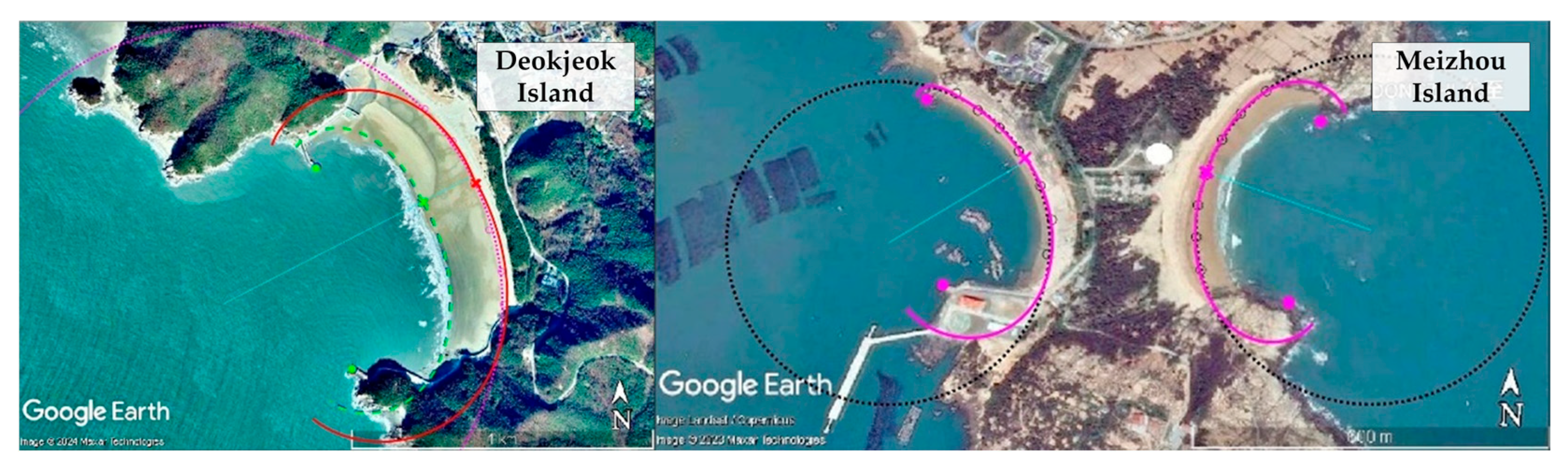
3.4. Bay Beaches with Asymmetrical Double Curvature

First, let us start with a simple case of asymmetrical double curvature for San Francisco Beach (36°32′40″ N, 4°36′56″ W) in Fuengirola (Figure 18), about 26 km SW of Málaga in Spain. By reproducing the prevailing wave direction for this beach (Elshinnawy et al. [61]), a local wave crest line (perpendicular to the wave direction) is drawn at each wave diffraction tip, and from there the basic wave angle of β₀ = 65.75° (Figure 5) is used to draw a pair of projection lines and the intersection becomes the common DCP (x). Each half of the static bay shape is then sketched using an updrift control point (o) and its corresponding downdrift control point (x). The resulting bay shape fits the existing shoreline planform well.

Following the same procedure for San Francisco in Spain (Figure 18) above, let us now see how to verify the planform of another asymmetrical double curvature in Rayong (12°39′28″ N, 101°16′09″ E) on the east coast of Thailand. Here, a moderately curved T-head groin with an over-developed tombolo exists between two external large fish-tailed groins 300 m apart (Figure 19). First, applying MeePaSoL to determine the prevailing wave direction and projecting a line shoreward using β₀ = 65.75° from each local wave crest line at the wave diffraction tip renders the intersection of a pair of two projection lines to become the common DCP “x”, as shown in Figure 19. Finally, all four shoreline planforms (large and small) within each large bay shape can be sketched using the common DCP. The whole process would take less than 5 min and the benefit is apparent, especially the saving in time and cost, compared with that using laboratory experiments and numerical models.

In addition, Pedregalejo (36°43′14″ N, 4°24′28″ E), about 4.5 km to the east of Málaga in Spain, was once a deserted fishing village, which has been transformed into a modern tourist hotspot since the 1980s, aided by artificial nourishment. A total of six asymmetrical bay shapes in double curvature (Figure 1 and Figure 20) have since been formed between three round-headed groins and a large detached breakwater or Y-shaped groin. Despite the smallness of the two little skewed bay shapes behind each round-headed groin, the whole process to verify the bay beach stability may take less than 10 min to complete. The overall benefit in saving time and cost to produce such a result is obvious, compared with that using laboratory studies and numerical models.

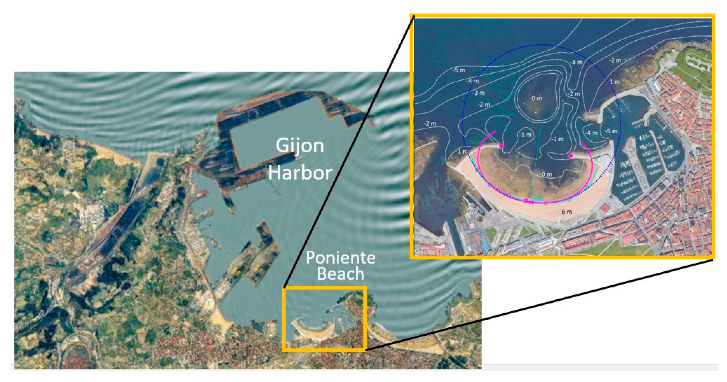
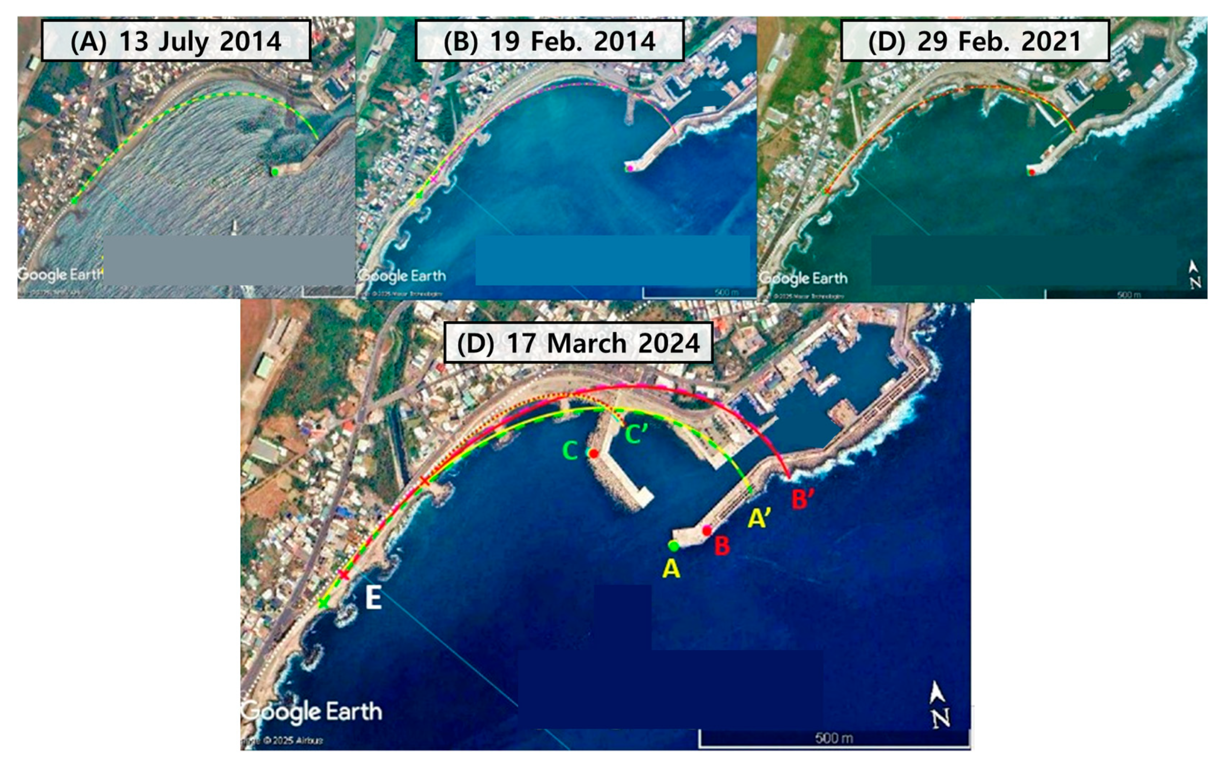
3.5. Beach Evolution and Protection Downdrift of Harbor Extension

Finally, the parabolic model is applied to demonstrate why the number of normal shore groins has been increased following the outer breakwater extension between 2014 and 2024 at Fugang Harbor (22°47′24″ N, 121°11′22 E) in the southeast coast of Taiwan (Figure 21). At each stage shown in Figure 21, the ideal shoreline predicted by the parabolic model (using the outer breakwater tip as the updrift control point) from March 2014 (Figure 21A) to February 2019 (Figure 21B), then in July 2021 (Figure 21C) and March 2024 (Figure 21D), were seaward in the lee of the breakwater, where accretion was anticipated accompanied by erosion further downdrift, thus calling for more groins to be constructed. On March 17, 2024 (Figure 21D), the predicted ideal stable planform EA’ remained in the water, implying local erosion will continue.

The above is a common scenario that has happened at many places in many countries. Traditionally, a similar topic could have been handled by a group of researchers or engineers using laboratory facilities, or a team of consultants applying advanced numerical packages. All involve large costs and manpower. However, it becomes apparent that the empirical parabolic model can be readily available to complement the work of the other two methods, even if it is in the preliminary planning stage. By siting the tip of the outer breakwater (e.g., point A in Figure 21D) to a proper location, it could be possible to match the ideal static bay shape with an existing shoreline planform to reduce the propensity for downdrift erosion and accretion behind, thus reducing the need to add more groins.

4. Discussion

4.1. Advantages of Empirical Geomorphic Model

All the HBB images presented in the present paper, whose planforms are fitted with the software MeePaSoL [37] for the parabolic model [35], are based on a geomorphic principle for a beach in static equilibrium that has its tangent at a downdrift shoreline perpendicular to the prevailing waves [47,48,49]. The visual results are then used to verify the stability of an existing bay beach or design a new beach, without resorting to wave conditions and bathymetry, which are necessary to run a numerical model, contrary to the example given by Tsai et al. [41] and Chen [42], who applied a combined hydrodynamic and morphodynamic model.

The results of hydrodynamic and morphodynamic processes are then calculated by a set of mathematical equations, without the knowledge of whether the resultant beach state (profile and planform) is in static equilibrium. The drawback is that the same wave conditions prevail constantly over a long duration of several hundred hours, months, or years. However, the morphodynamic process and outcome thus derived, although scientifically or technically “correct”, might not represent the “true” conditions in the field; we (coastal scientists, engineers, and managers) are willing to accept the calculated results only because no better approach is presently available. Wave motions in the ocean are a stochastic process. Nature has demonstrated its work in field conditions without using a statistical mean to represent the wave height and period (e.g., significant $H_{1/3}$ and $T_{1/3}$ or spectral peak period $T_p$) acting on a beach for engineering projects. This approach differs from the conventional laboratory tests and numerical models that use a specific set of statistical values of wave heights, periods, direction, and water levels (yet without the depth of the seabed).

Therefore, the method combining MeePaSoL and PBSE has the advantage of saving working time to produce a reliable graphic result of equilibrium shoreline within several minutes for each application. The benefit is apparent, compared to the strenuous efforts in time and cost experienced in applying laboratory tests or numerical models.

4.2. Issues Associated with Application of a Morphodynamic Modeling Study

The parabolic model has received recognition for project evaluation in the Shore Protection Manual [46], been integrated into the Spanish national Coastal Modeling System (SMC) [54], and been promoted in a special issue of Coastal Engineering [62]. However, several technical issues are worth further explanation for applying this model.

(1)

Timing of application and accuracy of results

González et al. [54] have recommended that the model can be applied at pre-design and design stages of a beach nourishment project in Spain. They also confirmed that the resulting beach “has still got a static equilibrium and remains pretty close to the predict equilibrium beach in plan and profile”, 10 years after its construction (Figure 9). The accuracy of the resulting tombolo planform with numerical modeling using XBeach can also be verified, as shown in Figure 11 and Figure 12 [41,42].

(2)

Applicable coastal landform types

The parabolic model is applicable to various sedimentary beaches, either sandy or coarse-grained, where headlands (natural or man-made) are in existence and are likely to form an embayed beach. Possible locations include downdrift of harbors, in the lee and behind detached breakwaters, downdrift of river-mouth jetties for navigation, in river-mouth spits, and in the vicinity of an offshore island. So far, applications have been found in estuarine deltas, such as that reported in Abdel Aziz [63], and in reverses spits.

(3)

Effects of water levels

Tidal levels are influencing factors for hydrodynamic and morphodynamic modeling (Rusdin et al. [64]). However, the parabolic model introduced in this paper can be applied to high and low water levels, without precise tidal-level analysis for the project site. Two examples are provided here to highlight the effect of the resulting planform on (i) Deokjeok Island in Gyeonggi-Do, Korea, and (ii) Meizhou Island in Fijian Province, China, as shown in Figure 22.

(4)

Material for headlands

For a stable HBB, the geometry of its headland (length, shape, size, orientation, and tip location) plays the most important role in transforming the incident wave field into combined wave diffraction–refraction patterns in the lee of the headland, helping sculpt the curved planform. Most natural headlands are rocky, monolithic, and rugged in shape and size, as well as deeply embedded into the seabed, while artificial headlands sit only 2–3 m below the sea floor, thus inducing scouring, sinking, and instability. Although artificial headlands are made of granite rocks or precast concrete blocks, the function of the headland does not depend on the type of solid block, instead depending on the tip of the headland where wave diffraction takes place. Therefore, whether a headland is constructed with tetrapods, dolosse, Accropods, Core-Locs, or antifers (Mousavi et al. [65]), a similar resulting planform would occur, as depicted in Figure 23, where granite rocks are in use in Montechiaro in Italy.

(5)

Complexity of coastal landform

The parabolic model with the MeePaSoL software is applicable to complex coastal planforms, with sound knowledge of wave transformation, the relation between predominant wave direction and shoreline orientation, the effect of offshore islands, and the geomorphic principles of wave diffraction. As shown in Figure 24, the ideal static bay shape predicted by the wave diffraction point at P₁ on Tamandúa Island is E₁–C₁ and that at P₂ on Cocanha Island is E₂–C₂. Despite curve E₂–C₂ being in good agreement with the salient in the lee of Cocanha Island, E₁–C₁ deviates from the north part of the existing beach planform, suggesting the potential for salient formation and erosion heading northward from the central part of the beach.

4.3. Case Study

A large yacht marina exists in Agios Nikolaos (35°11′10″ N, 25°43′04″ E) in the northeast of Crete, Greece (Figure 25A), showing the solid outer breakwater for the marina and three detached breakwaters (Figure 25B), together with one salient and Ammos Beach (the main beach). Using the sandy beach features (Ammos Beach and the salient) in Figure 25C, could we provide a reasonable answer to questions 1 and 2 marked in the figure, without resorting to numerical modeling (hydrodynamic and morphodynamic models)?

As shown in Figure 26, if detached breakwater BC is constructed first, a tombolo could form (curves B₁ and C₁), with sufficient sediment supply, or a small salient if sediment is limited. However, both scenarios cannot exist because the existing salient is skewed. Alternatively, if the emergent outer breakwater for the marina is constructed first, planform A₁ could form, using tip A as a wave diffraction point. Interestingly, curve A₁ matches nicely with the southern side of the salient. In the lee of the marina, the wave direction changes and propagates toward the main beach B₂. However, with tip B as the wave diffraction point, it could end up on the northern side of the existing salient, B₂, and the curve could fit the main beach.

Therefore, by applying the knowledge of wave diffraction, together with the geomorphic principle between the prevailing wave direction and the planform of a beach in equilibrium, we may derive an applaudable conclusion, as illustrated.

5. Concluding Remarks

Almost all the coastal landforms that nature display along the oceanic edge are in equilibrium with their external forcings and morphodynamic response, until that stability is interfered with by human action. This often results in a change to wave fields and discontinuity in sediment transport, causing beach erosion. To investigate the potential adverse effects, coastal scientists and researchers have conducted laboratory experiments in wave basins and developed various hydrodynamic models and morphodynamic models in recent times.

However, as the scale (dimensions) of the project increases, a large basin is needed to operate, but it still cannot determine when equilibrium is reached to terminate the test. A similar drawback is associated with running a program applied to numerical modeling. On the contrary, the empirical parabolic model derived for HBBs in static equilibrium can be taken to complement the numerical modeling, because its results can be obtained readily by the MeePaSoL software, which supports the empirical model. To prevent beach erosion behind detached breakwaters, adequate nourishment can be applied to produce the planform given by the parabolic model, thereby accelerating the stability of the new beach.

For the application of the empirical model, González et al. [30] have identified that the model is useful for supporting different operational levels (pre-design and design) of HBB in coastal engineering projects (including beach nourishment designs), as well as for academic purposes. They cited a successful example of the application of this methodology to a project on Poniente Beach (Gijón) in Spain, stating that the beach has remained in static equilibrium pretty close to the predicted equilibrium beach in planform and profile.

From the various examples demonstrated in this paper, we are confident that the parabolic model has the advantage over laboratory tests and the combined hydrodynamic and morphodynamic models for predicting an HBB in equilibrium. The graphic results of shoreline planforms can be produced within a couple of minutes, without input of wave conditions or bathymetry, and have adequate accuracy for preliminary design. By combining the parabolic model with laboratory tests and numerical modeling, we believe the teamwork would improve the efficiency and reliability of an engineering project.

Software Availability for MeePaSoL

-

Developer: Laboratory of Coastal Environment, Sungkyunkwan University (SKKU), Republic of Korea. Group leader: Professor Jung L. Lee.

-

Program language: The code is written in MATLAB.

-

Access to source code: https://github.com/BSMC-20180404/MeePaSoL.git (accessed on 06 May 2022).

-

The MATLAB codes in MeePaSoL.zip (download from the link) can be run as a compiled standalone execution document without installing the bulk of the MATLAB system, after downloading and installing “matlab runtime” MCR version 2021a (9.10) for Windows (64-bit), from MathWorks’ homepage, https://www.mathworks.com, onto a computer.

-

Key references for software applications: Lim et al. [37] and Lee et al. [34].

References

1. Vitousek, S.; Barnard, P.; Limber, P.; Erikson, L.; Cole, B. A model integrating longshore and cross-shore processes for predicting long-term shoreline response to climate change. J. Geophys. Res. Earth Surf. 2017, 122, 782–806. [Google Scholar] [CrossRef]
2. Kamphuis, J.W. Introduction to Coastal Engineering and Management; Advanced Series on Ocean Engineering; World Scientific: Singapore, 2010; Volume 30, 525p. [Google Scholar]
3. Warren, I.R.; Bach, H. Mike 21: A modelling system for estuaries, coastal waters and seas. Environ. Softw. 1992, 7, 229–240. [Google Scholar] [CrossRef]
4. Roelvink, J.A.; Van Banning, G.K.F.M. Design and development of DELFT3D and application to coastal morphodynamics. Oceano. Lit. Rev. 1995, 11, 925. [Google Scholar]
5. Hanson, H. GENESIS—A Generalized Shoreline Change Numerical Method. J. Coast. Res. 1989, 5, 1–27. [Google Scholar]
6. Hanson, H.; Kraus, N.C. Genesis: Generalized Model for Simulating Shoreline Change; Coastal Engineering Research Center: Vicksburg, MS, USA; U.S. Army Corps of Engineers: Washington, DC, USA, 1989; CERC-MP-89-19. [Google Scholar]
7. Larson, M.; Kraus, N.C. SBEACH: Numerical Model for Simulating Storm-Induced Beach Change, Report 1, Empirical Foundation and Model Development; Coastal Engineering Research Center: Newark, NJ, USA; U.S. Army Corps of Engineers: Washington, DC, USA, 1989; Report CERC-89-9. [Google Scholar]
8. Larson, M.; Kraus, N.C.; Byrnes, M.R. SBEACH: Numerical Model for Stimulating Storm-Induced Beach Change; Coastal Engineering Research Center: Newark, NJ, USA; U.S. Army Corps of Engineers: Washington, DC, USA, 1989; Report CERC-89-9. [Google Scholar]
9. Roelvink, D.; Reniers, A.; van Dongeren, A.; van Thiel de Vries, J.; Lescinski, J.; McCall, R. XBeach Model Description and Manual; UNESCO-IHE Institute for Water Education, Deltares and Delft University of Technology: Delft, The Netherlands, 2010; Report 21 June 2010. [Google Scholar]
10. Warner, J.C.; Armstrong, B.; He, R.; Zambon, J.B. Development of a coupled ocean-temperature-wave-sediment transport (COAWST) modelling system. Ocean Model. 2010, 35, 230–244. [Google Scholar] [CrossRef]
11. Bruun, P. The Bruun rule of erosion by sea-level rise: A discussion on large-scale two-dimensional usages. J. Coast. Res. 1988, 4, 627–648. [Google Scholar]
12. Miller, J.K.; Dean, R.G. A simple shoreline change model. Coast. Eng. 2004, 51, 531–556. [Google Scholar] [CrossRef]
13. Yates, M.L.; Guza, R.T.; O’Reilly, W.C. Equilibrium shoreline response: Observations and Modeling. J. Geophys. Res. 2009, 114, C09014. [Google Scholar] [CrossRef]
14. Yates, M.L.; Guza, R.T.; O’Reilly, W.C.; Hansen, J.E.; Barnard, P.L. Equilibrium shoreline response of a high wave energy beach. J. Geophys. Res. 2011, 116, C04114. [Google Scholar] [CrossRef]
15. Davidson-Arnott, R.G. Conceptual model of the effect of sea level rise on sand coasts. J. Coast. Res. 2005, 21, 1166–1172. [Google Scholar] [CrossRef]
16. Davidson, M.A.; Lewis, R.P.; Turner, I.L. Forecasting of seasonal to multi-year shoreline change. Coast. Eng. 2010, 57, 620–629. [Google Scholar] [CrossRef]
17. Splinter, K.D.; Turner, I.L.; Davidson, M.A.; Barnard, P.; Castelle, B.; Otman-Shay, J. A generalized equilibrium model for predicting daily to interannual shoreline response. J. Geophys. Res. 2014, 119, 1936–1958. [Google Scholar] [CrossRef]
18. Pelnard-Considère, R. Essai de théorie de l’évolution des formes de rivage en plages de sable et de galets. Journées L’hydraulique 1957, 4, 289–298. [Google Scholar]
19. Larson, M.; Hanson, H.; Kraus, N.C. Analytical solution of one-line model for shoreline change near coastal structure. J. Waterw. Port Coast. Ocean Eng. 1997, 39, 180–191. [Google Scholar] [CrossRef]
20. Ashton, A.; Murray, A.B.; Arnoult, O. Formation of coastline features by large-scale instabilities induced by high-angle waves. Nature 2001, 414, 296–300. [Google Scholar] [CrossRef]
21. Ashton, A.D.; Murray, A.B. High-angle wave instability and emergent shoreline shapes: 1. Modelling of sand waves, flying spits, and capes. J. Geophys. Res. 2006, 111, FD4011. [Google Scholar] [CrossRef]
22. Reeve, D.; Chadwick, A.; Fleming, C. Coastal Engineering: Processes, Theory and Design Practice, 2nd ed.; Spon Press, Taylor & Francis: London, UK, 2012; 514p. [Google Scholar]
23. U.S. Army Corps of Engineers (USACE). Shore Protection Manual; Coastal Engineering Research Center: Washington, DC, USA, 1984. [Google Scholar]
24. Kamphuis, J.W.; Davies, M.H.; Nairn, R.B.; Sayao, O.J. Calculation of littoral sand transport rate. Coast. Eng. 1986, 10, 1–21. [Google Scholar] [CrossRef]
25. Kamphuis, J.W. Alongshore sediment transport rate. J. Waterw. Port Coast. Ocean Eng. 1991, 117, 624–640. [Google Scholar] [CrossRef]
26. Inman, D.L.; Nordstrom, C.E. On the tectonic and morphologic classification of coasts. J. Geol. 1971, 79, 1–21. [Google Scholar] [CrossRef]
27. Short, A.; Masselink, G. Embayed and structurally controlled beaches. In Handbook of Beach and Shoreface Morphodynamics; Short, A., Ed.; Wiley: Chichester, UK, 1999; pp. 230–250. [Google Scholar]
28. Silvester, R. Stabilization of sedimentary coastline. Nature 1960, 4749, 467–469. [Google Scholar] [CrossRef]
29. Silvester, R.; Ho, S.K. Use of crenulate shaped bays to stabilize coasts. Coast. Eng. 1972, 2, 1347–1365. [Google Scholar]
30. González, M.; Medina, R.; Losada, M. On the design of beach nourishment projects using static equilibrium concepts: Application to the Spanish coast. Coast. Eng. 2010, 57, 227–240. [Google Scholar] [CrossRef]
31. Yamashita, T.; Tsuchiya, Y. Numerical simulation of pocket beach formation. Coast. Eng. 1992, 196, 2556–2566. [Google Scholar]
32. Lim, C.; Lee, J.; Lee, J.L. Simulation of bay-shaped shorelines after the construction of large-scale structures by using a parabolic bay shape equation. J. Mar. Sci. Eng. 2021, 9, 43. [Google Scholar] [CrossRef]
33. Silva, R.; Baquerizo, A.; Losada, M.Á.; Mendoza, E. Hydrodynamics of a headland-bay beach—Nearshore current circulation. Coast. Eng. 2010, 57, 160–175. [Google Scholar] [CrossRef]
34. Lee, J.L.; Lim, C.; Pranzini, E.; Yu, M.J.; Chu, J.C.; Chen, C.J.; Hsu, J.R.C. Assessing downdrift control point and asymmetric double-curvature planform behind multiple detached breakwaters: Simple empirical method. Coast. Eng. 2023, 185, 104361. [Google Scholar] [CrossRef]
35. Hsu, J.R.C.; Evans, C. Parabolic bay shapes and applications. Proc. Inst. Civ. Eng. 1989, 87, 557–570. [Google Scholar] [CrossRef]
36. Klein, A.H.F.; Vargas, A.; Raabe, A.L.A.; Hsu, J.R.C. Visual assessment of bayed beach stability using computer software. Comput. Geosci. 2003, 29, 1249–1257. [Google Scholar] [CrossRef]
37. Lim, C.B.; Hsu, J.R.C.; Lee, J.L. MeePaSoL: A MATLAB-based GUI software tool for shoreline management. Comput. Geosci. 2022, 161, 105059. [Google Scholar] [CrossRef]
38. Rausman, R.; Klein, A.H.F.; Stive, M.J.F. Uncertainty in the application of the parabolic bay shape equation: Part 1. Coast. Eng. 2010, 57, 132–141. [Google Scholar] [CrossRef]
39. Rausman, R.; Klein, A.H.F.; Stive, M.J.F. Uncertainty in the application of the parabolic bay shape equation: Part 2. Coast. Eng. 2010, 57, 142–151. [Google Scholar] [CrossRef]
40. Silvester, R. Natural headland control of beaches. Cont. Shelf Res. 1985, 4, 581–596. [Google Scholar] [CrossRef]
41. Tsai, C.P.; Chen, Y.C.; Ko, C.H. Prediction of bay-shaped shorelines between detached breakwaters with various gap spacings. Sustainability 2023, 15, 6218. [Google Scholar] [CrossRef]
42. Chen, Y.C. Prediction of Bay-Shaped Shoreline and Storm Beach Buffer Width between Two Offshore Breakwaters. Doctoral Dissertation, Department of Civil Engineering, National Chung Hsing University, Taichung, Taiwan, 2024. [Google Scholar]
43. Yasso, W.E. Plan geometry of headland-bay beaches. J. Geol. 1965, 73, 702–714. [Google Scholar] [CrossRef]
44. Moreno, L.J.; Kraus, N.C. Equilibrium shape of headland-bay beaches for engineering design. Proc. Coast. Sedi. 1999, 1, 860–875. [Google Scholar]
45. Kemp, J.; Vandeputte, B.; Eccleshall, T.; Simos, R.; Troch, P. A modified hyperbolic tangent equation to determine equilibrium shape of headland-bay beaches. Coast. Eng. 2018, 16, 106. [Google Scholar] [CrossRef]
46. USACE. Shore Protection Manual Online; Technical Note 1-61, U.S.; U.S. Army Corps of Engineers: Washington, DC, USA; Government Printing Office: Washington, DC, USA, 2002; pp. 35–56, Part III-2 54–56 & Part V-3 35–43. [Google Scholar]
47. Lewis, W.V. The evolution of shoreline curves. Proc. Geol. Assess. 1938, 49, 107–126. [Google Scholar] [CrossRef]
48. Jennings, J.N. The influence of wave action on coastline outline in plan. Aust. Geogr. 1955, 6, 36–44. [Google Scholar] [CrossRef]
49. Davies, J.L. Wave refraction and the evolution of shoreline curves. Geogr. Stud. 1958, 5, 1–14. [Google Scholar]
50. Tan, S.K.; Chiew, Y.M. Analysis of bayed baches in static equilibrium. J. Waterw. Port Coast. Ocean Eng. 1994, 120, 145–153. [Google Scholar] [CrossRef]
51. Uda, T.; Serizawa, M.; Kumada, T.; Sakai, K. A new model for predicting three-dimensional beach changes by expending Hsu and Evans’ equation. Coast. Eng. 2010, 57, 194–202. [Google Scholar] [CrossRef]
52. Lee, J.L. MeePaSoL: MATLAB-GUI Based Software Package; Sungkyunkwan University: Seoul, Republic of Korea, 2015; SKKU Copyright No. C-2015-02461. [Google Scholar]
53. González, M.; Medina, R. On the application of static equilibrium bay formulations to natural and man-made beaches. Coast. Eng. 2001, 43, 209–225. [Google Scholar] [CrossRef]
54. González, M.; Medina, R.; González-Ondina, J.; Osorio, A.; Méndez, F.J.; García, E. An integrated coastal modelling system for analyzing beach processes and beach restoration projects, SMC. Comput. Geosci. 2007, 33, 916–931. [Google Scholar] [CrossRef]
55. Dean, R.G. Equilibrium beach profiles: Characteristics and applications. J. Coast. Res. 1991, 7, 53–84. [Google Scholar]
56. Roelvink, J.A. Coastal morphodynamic evolution technique. Coast. Eng. 2006, 53, 277–287. [Google Scholar] [CrossRef]
57. Roelvink, D.; Van Dongeren, A.; McCall, R.; Hoonhout, B.; van Rooijen, A.; van Geer, P.; de Vet, P.; Nederhoff, K.; Quataret, E. Technical Reference: Kingsday Release (Technical Report: Model Description and Reference Guide to Functionalities); Deltares, UNESCO-IHE Institute of Water Education and Delft University of Technology: Delft, The Netherlands, 2015; p. 141. [Google Scholar]
58. Roelvink, D.; Reniers, A.; van Dongeren, A.; van Thiel de Vries, J.; McCall, R.; Lescinski, J. Modelling storm impacts on beaches, dune and barrier islands. Coast. Eng. 2009, 56, 1133–1152. [Google Scholar] [CrossRef]
59. Khuong, T.C. Shoreline Response to Offshore Breakwaters in Prototype. Ph.D. Thesis, Department of Hydraulic Engineering, Delft University of Technology, Delft, The Netherlands, 2016; 148p. [Google Scholar]
60. Lim, C.; Lee, J.L.; Hsu, J.R.C. Mitigating shoreline retreat between multiple detached breakwaters: Empirical and semi-analytical approach. Appl. Ocean. Res. 2025, 154, 104385. [Google Scholar] [CrossRef]
61. Elshinnawy, A.I.; Medina, R.; González, M. Equilibrium planform of pocket beaches behind breakwater gaps: On the location of the intersection point. Coast. Eng. 2022, 173, 104096. [Google Scholar] [CrossRef]
62. Hsu, J.R.C.; Yu, M.J.; Lee, F.C.; Benedet, L. Static bay beach concept for scientists and engineers: A review. Coast. Eng. 2010, 57, 76–91. [Google Scholar] [CrossRef]
63. Abdel Aziz, K.M. Quantitative monitoring of coastal erosion and changes using remote sensing in a Mediterranean delta. Civ. Eng. J. 2024, 10, 1842–1862. [Google Scholar] [CrossRef]
64. Rusdin, A.; Oshikawa, H.; Divanesia, A.M.A.; Hatta, M.P. Analysis and prediction of tidal measurement data from temporary stations using the least squares method. Civ. Eng. J. 2024, 10, 384–403. [Google Scholar] [CrossRef]
65. Mousavi, S.H.; Kavianpour, M.R.; Yamini, O.A. Experimental analysis of breakwater stability with antifer concrete block. Mar. Georesour. Geotechnol. 2017, 35, 426–434. [Google Scholar] [CrossRef]
Figure 1. Complex asymmetrical embayments at Pedregalejo east of Málaga in Spain (courtesy of Google Earth; images from June 2018).
Jmse 13 01053 g001
Figure 2. Definition sketch of the parabolic model for a bay beach in static equilibrium [35].
Jmse 13 01053 g002
Figure 3. Best-fit curves for the three original C coefficients in the parabolic bay shape equation [35], showing additional prototype data to verify the applicability of the model.
Jmse 13 01053 g003
Figure 4. Definition sketch of parameters for multiple DBWs at equal distance offshore under normal wave incidence, showing symmetrical double curvatures with a common DCP at β0 = 65.75° [34].
Jmse 13 01053 g004
Figure 5. Layout of multiple DBWs at unequal distance offshore under normal wave incidence, showing a triangle set up by lines of β0 = 65.75° from each breakwater tip for asymmetrical double curvature with a common DCP at P [34].
Jmse 13 01053 g005
Figure 6. Flowchart depicting the procedure (a series steps) in the MATLAB program for applying MeePaSoL, shown in the logo in Figure 7 [37].
Jmse 13 01053 g006
Figure 7. Output of the SEP (solid line) and predominant wave direction determined by the software MeePaSoL for Diazville Beach in South Africa, showing points (small black “o”s) for shoreline digitizing and the common DCP at E (“o”). (Image courtesy of Google Earth in August 2016) [37].
Jmse 13 01053 g007
Figure 9. Embayed Poniente Beach inside Gijón Harbor designed using SMC, showing complex bathymetry and depression for wave transformation toward the beach, with a solid magenta line for the output of the parabolic model from the blue fitted circle [35].
Jmse 13 01053 g009
Figure 10. Wave basin and experimental setup with two detached breakwaters (black solid lines at the top) used by Chen [42].
Jmse 13 01053 g010
Figure 11. Temporal and spatial variations in wave height and water level (left panels) plus current patterns and sediment transport (right panels) for S o /G = 1.0 and a total duration of 30 months [42].
Jmse 13 01053 g011
Figure 12. Temporal process from a salient to an over-developed tombolo for S o /G = 1.0 and H i = 1.3 m, showing the final planform verified using the parabolic model [35,41,42].
Jmse 13 01053 g012
Figure 13. Comparison on the simulated final equilibrium shoreline planform for over-developed tombolos with various gaps S o /G [41,42].
Jmse 13 01053 g013
Figure 14. Modified relationship between the final and initial shoreline distance S/G versus S o /G, redrawn from simulated data N1–N5 [41,42] and field data from Khuong [59].
Jmse 13 01053 g014
Figure 15. Maximum dimensionless shoreline retreat b/ S o versus relative shoreline distance S o /S [60], based on simulated data N1–N5 [41,42] and field data [59].
Jmse 13 01053 g015
Figure 16. Bay beaches in symmetrical double curvature behind detached breakwaters at Rayong west in Thailand (Google Earth from April 2023).
Jmse 13 01053 g016
Figure 17. São Martinho do Porto Beach in Portugal, showing an almost semi-circular planform deep behind a narrow opening (Google Earth from August 2019).
Jmse 13 01053 g017
Figure 18. Verification of asymmetrical bay shape in double curvature for San Francisco in southern Spain (Google Earth image from June 2017).
Jmse 13 01053 g018
Figure 19. Verification of asymmetrical bay shapes in double curvature at Rayong in Thailand (beach image courtesy of Google Earth from August 2019).
Jmse 13 01053 g019
Figure 20. Verification of asymmetrical bay shapes in double curvature at Pedregalejo in Spain (beach image courtesy of Google Earth from June 2018).
Jmse 13 01053 g020
Figure 21. Evolution of the shoreline change at Fugang Harbor in Taiwan from 2014 to 2024, showing progressive installation of the outer breakwater and protective groins: (A) 13 July 2014; (B) 19 February 2014; (C) 29 February 2021; (D) 17 March 2024 (beach image courtesy of Google Earth).
Jmse 13 01053 g021
Figure 22. Resulting shoreline planform on (left) Deokjeok Island in Gyeonggi-Do, Korea, and (right) Meizhou Island in Fijian Province, China, where the tidal range is about 4 m and the static planform is fitted using MeePaSoL (image courtesy of Google Earth).
Jmse 13 01053 g022
Figure 23. Resulting shoreline planform with granite rocks in Montechiaro in Naples, Italy (image courtesy of Google Earth; date: 22 June 2022).
Jmse 13 01053 g023
Figure 24. Resulting shoreline planforms from MeePaSoL, showing predominant wave direction and predicted static bay shapes E1-C1 and E2-C2 compared with the existing planform for Massaguaçu Beach in Brazil (image courtesy of Google Earth; date: 31 August 2018).
Jmse 13 01053 g024
Figure 25. Formation of the salient and the embayed beach in Agios Nikolaos in Greece: (A) Large-scale view; (B) medium-scale view; and (C) detailed (zoomed-in) view (Google Earth image from February 2024 and #MyAgiosNilolaosCrete).
Jmse 13 01053 g025
Figure 26. Static bay shapes predicted by the parabolic model using tips A, B, and C to match the under-developed salient behind detached breakwater BC and bay beach B2 at Agios Nikolaos in Greece (Google Earth image from February 2024).
Jmse 13 01053 g026
Disclaimer/Publisher’s Note: The statements, opinions and data contained in all publications are solely those of the individual author(s) and contributor(s) and not of MDPI and/or the editor(s). MDPI and/or the editor(s) disclaim responsibility for any injury to people or property resulting from any ideas, methods, instructions or products referred to in the content.