Seismic Prediction of Shallow Unconsolidated Sand in Deepwater Areas

Abstract

Recently, shallow gas fields and hydrate-bearing sand in the deepwater area of the northern South China Sea have been successively discovered, and the accurate prediction of shallow sands is an important foundation. However, most of the current prediction methods are mainly for deep oil and gas reservoirs. Compared with those reservoirs with high degree of consolidation, shallow sandy reservoirs are loose and unconsolidated, whose geophysical characteristics are not well understood. This paper analyzes the logging data of shallow sandy reservoirs recovered in the South China Sea recently, which show that the sand content has a significant influence on Young’s modulus and Poisson’s ratio of the sediments. Therefore, this paper firstly constructs a new petrophysical model of unconsolidated strata targeting sandy content and qualitatively links the mineral composition and the elastic parameters of the shallow marine sediments and defines a new indicator for sandy content: the modified brittleness index (MBI). The effectiveness of MBI in predicting sandy content is then verified by measured well data. Based on pre-stack seismic inversion, the MBI is then inverted, which will identify the sandy deposits. The method proposed provides technical support for the subsequent shallow gas and hydrate exploration in the South China Sea.

1. Introduction

Marine shallow sandy sediments are favorable reservoirs for shallow gas and gas hydrates [1,2,3,4], because when free gas enters a reservoir, free gas preferentially flows into the coarse-grained layers because the coarse-grained layers have low capillary entry pressures [5] (e.g., <0.1 MPa). However, free gas cannot enter the interbedded muds because the muds usually have much higher capillary entry pressures [5,6] (e.g., >1 MPa). In 2019–2023, the China Geological Survey discovered sandy hydrates at a shallow sand near at about 130 m below the seafloor (mbsf) in the Qiongdongnan basin, South China Sea [7], and in 2024 CNOOC discovered the LS36-1 shallow gas field in western Qiongdongnan Basin, where the gas layer is mainly located at 170–300 mbsf [8], accurate prediction of shallow sand is an important foundation for realizing the above exploration breakthroughs. Additionally, hydrate-bearing sand and shallow gas systems store significant amounts of methane as a huge marine carbon sink, which also supply gas for cold seep worldwide. They are a part of the global carbon cycle interacting with the global climate [9,10,11,12]. Moreover, large-scale gases release from hydrate dissociation can trigger submarine landslides [13]. Thus, predicting shallow sand layers holds great scientific importance.

Currently, the identification of sandy reservoir mainly relies on the interpretation of seismic sedimentary facies [14], but the results are subject to some uncertainties due to the complexity of the seismic response. Generally, sand layers exhibit higher P-wave velocity and density than surrounding clays, resulting in continuous positive-polarity reflections on seismic profiles [15]. However, shallow unconsolidated sand with higher porosity may also have lower velocities than surrounding clays depending on the sand content [16,17], leading to negative-polarity reflections. Additionally, gas or gas hydrates may be present in these sands. The velocities of gas- or hydrate-bearing sands with different saturation cause varying degrees of velocity changes [18], making interpretation more challenging. Seismic inversion may be an effective means to accurately predict sandy reservoir [19,20,21,22]. Previous studies have shown that the mechanical properties of sediments are sensitive to sand content, and the main component of sand is quartz, which is one of the brittle minerals. Rickman et al. [23] performed statistics on several wells in the Barnett Shale area and obtained a map of the relationship between formation brittleness and rock mineral fractions. Sondergeld et al. [24,25] proposed a relationship between formation brittleness and rock mineral fractions that a high brittleness is associated with a larger content of brittle minerals, and quartz, feldspar, calcite, and hydrate-associated pyrite and carbonatite are all related to brittleness. However, the shallow marine sediments have not yet been consolidated, and the geophysical characteristics are of special nature, especially for the ultra-shallow sand bodies in the deep-water area.

In addition, hydrates may occur in shallow marine sands, and the velocity of hydrate-bearing sands increase [26,27], and fee gas causes velocity reduction and frequency amplitude attenuation [28], which will affect the evaluation of sand content using seismic inversion [29]. These characteristics can be modeled by rock physics. Hydrates cementing sand grains will significantly increase the P-wave velocity, and the classic cementation model [30] can be used to link the hydrate saturation and cementing radius to elastic velocities. We can also use effective medium theory [31] or the three-phase Biot equation (TPBE) [32] to model the velocity of the hydrate-bearing sand, assuming that hydrate is part of the matrix. However, these models ignore the intergrain friction across the Hertzian contact area [33], and it often overpredicts the S-wave velocity. There was also a lack of actual logging and drilling data before, and these models are not well constrained [34,35]. Therefore, unconsolidated characteristics and the occurrences of hydrate and free gas need to be taken into account for the prediction of shallow marine sands.

In this paper, we first consider the geophysical characteristics of unconsolidated sediments by integrating the Hertz–Mindlin (H-M) contact model [36] and the anisotropic petrophysical model, then we analyze the impacts of sandy content, grain size, and gas and hydrate saturation on the elastic parameter, and we propose a new indicator for sandy reservoir: the modified brittleness index (MBI). The scientific validity of this indicator is analyzed by well log data acquired recently in the South China Sea. Finally, we use pre-stack seismic inversion to obtain the MBI, and the results are consistent with logging and drilling results.

2. Materials and Methods

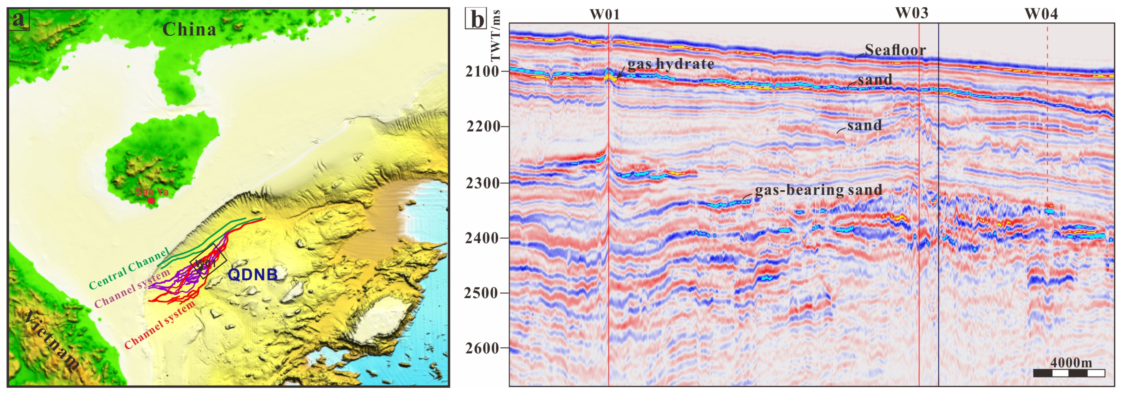
2.1. Geological Settings

The Qiongdongnan Basin (QNDB), situated in the western sector of the northern South China Sea (Figure 1a). This basin hosts proven hydrocarbon accumulations including the LS17-2 gas field and LS36-1 shallow gas field [8,37]. The Guangzhou Marine Geological Survey (GMGS) has also carried out successive hydrate drilling expeditions (GMGS5-GMGS8, 2018–2022) for the shallow marine gas hydrate occurrences targeting Neogene-Quaternary sedimentary sequences [38,39].

Hydrate-bearing core samples were obtained from Pleistocene strata in wells W01 and W03 (Figure 1b) [40]. The QDNB hosts syntectonic channel complexes and associated depositional architectures within Neogene sequences, as evidenced by extensive seismic stratigraphic analyses [41]. Modern sedimentological investigations reveal stacked six Late Quaternary channel-levee systems in shallow sedimentary packages, comprising four principal lithofacies [42,43]. These stratigraphic conduits serve as hydrocarbon migration pathways, with buoyancy-driven fluid migration preferentially utilizing high-permeability channel sands for vertical hydrocarbon transport.

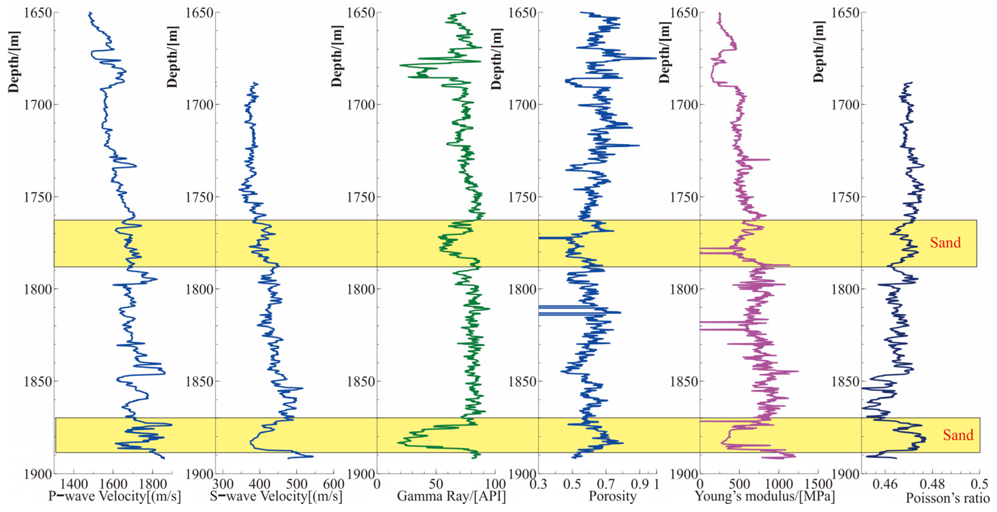
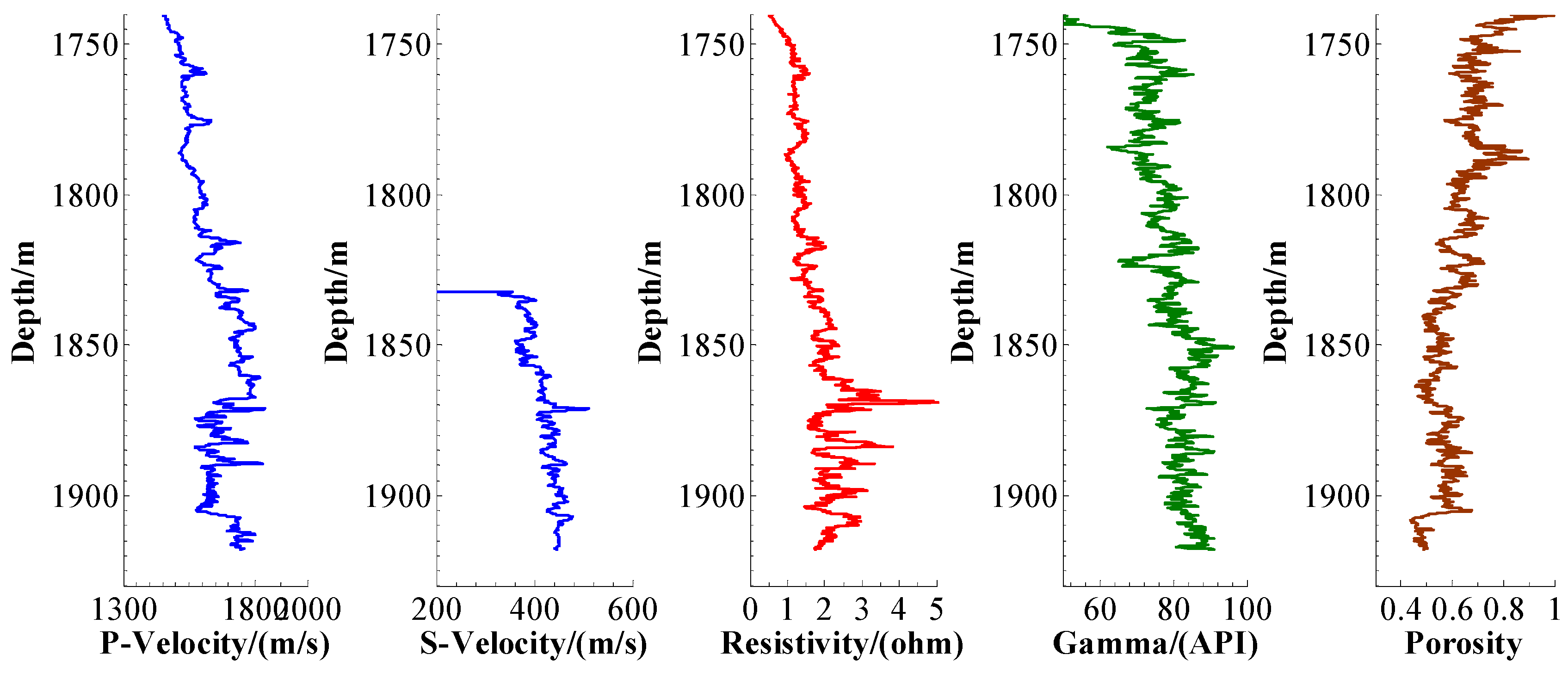
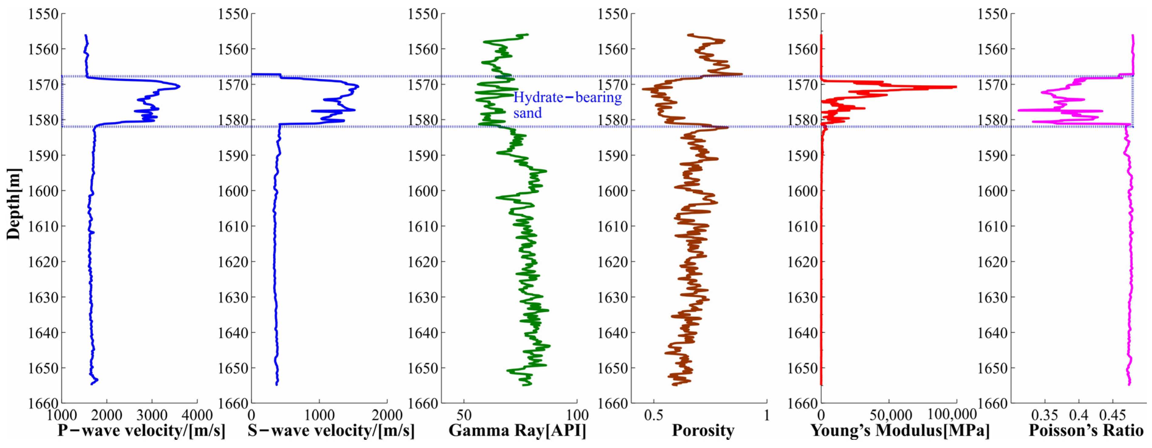
2.2. Well Logs and Seismic Data

A comprehensive set of high-quality logging-while-drilling (LWD) measurements was successfully obtained during the operation. The acquired dataset comprised key measurements including caliper, penetration rate, natural gamma radiation, resistivity, bulk density, neutron porosity, acoustic waveforms, and nuclear magnetic resonance (NMR). Following data acquisition, an integrated analytical workflow was executed to characterize hydrate-bearing formations through sequential operations: elastic wave velocity analysis and elemental analysis (ELAN)-based reservoir assessment, combined with specialized processing and interpretation of both nuclear magnetic and resistivity image data. Additional petrophysical evaluations incorporated elemental spectral analysis and neutron capture cross-section measurements, all performed according to Schlumberger’s established protocols to quantify hydrate saturation, pore space distribution, and lithological constituents.

The 3D seismic acquisition employed a triple-source, 12-streamer configuration with 5100 m streamers deployed at 75 m lateral intervals, maintaining a 5 m tow depth. Airgun arrays with a total volume of 2030 in³ were positioned at 4 m subsurface depth, generating seismic energy sampled at 1 ms intervals with 68-fold coverage.

The processing sequence incorporated zero-phase wavelet correction, ghost wavefield attenuation, surface-related multiple elimination, followed by both pre-stack time and depth migration techniques. The dataset exhibits an operational bandwidth of 5–85 Hz with a dominant frequency peak at 58 Hz, preserving positive polarity seabed reflections critical for identifying key geological features including bottom-simulating reflectors (BSR), hydrate phase boundaries, sand deposits, and stratigraphic discontinuities.

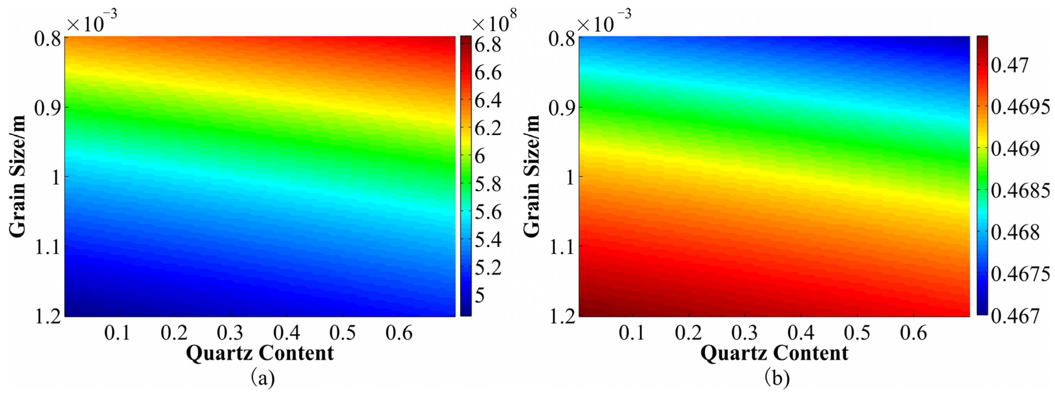
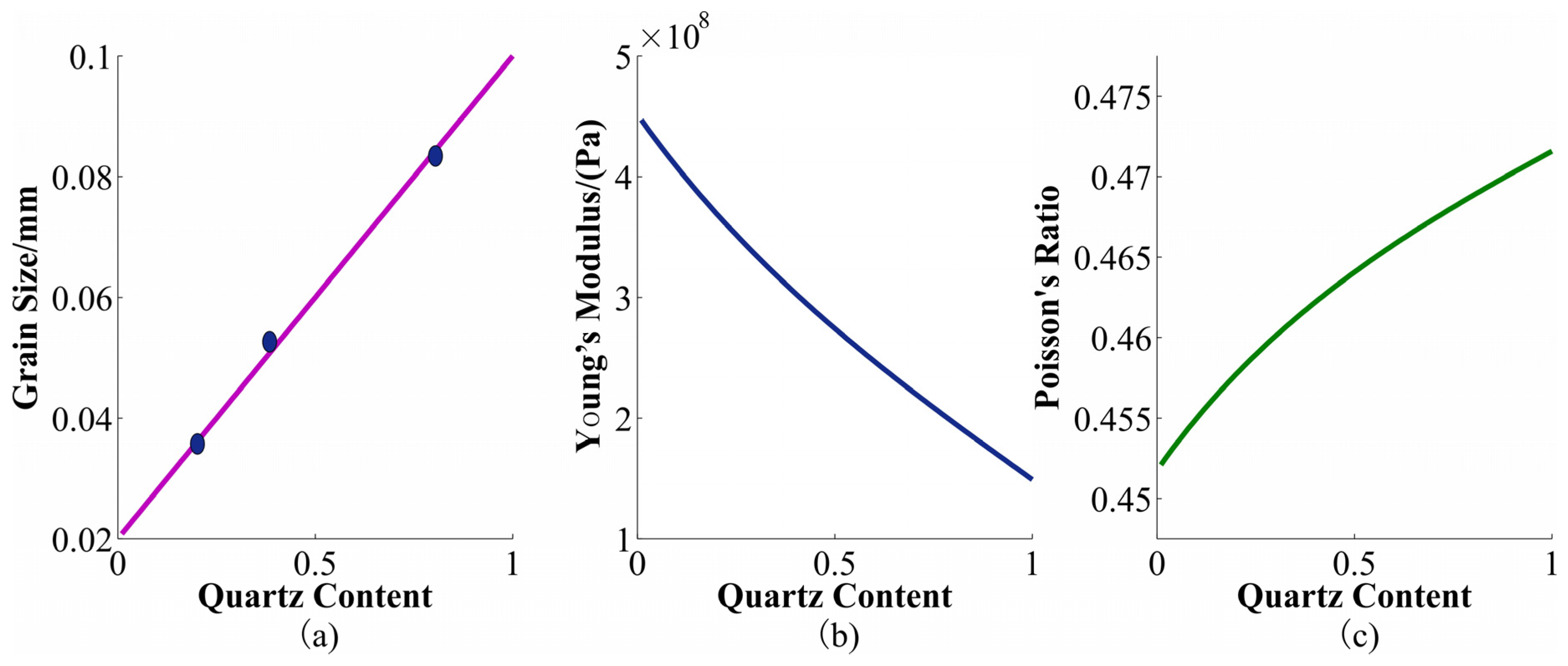
2.3. Rock Physics Modeling

Unconsolidated clastic sandstone has a granular structure. It consists of particles like quartz and feldspar, which form a rock framework through certain contact modes. In essence, it is a soft condensed material of many discrete particles. Adjacent particles interact via contact deformation to transmit energy. A key feature of unconsolidated sediments is that particles can slide relative to each other under stress. Under specific boundary conditions, tangential forces do not just cause tangential movement for local equilibrium. Instead, they generate torques on particle centers. Under these torques, contacting particles rotate and rearrange locally without tangential displacement increments. These particle motions can also make the resultant force on particles zero, achieving local equilibrium and causing stress relaxation in the medium. The H-M particle contact model is used to characterize the equivalent modulus of unconsolidated sediments in this case [44,45]. Based on the physical property of hydrate reservoirs, we built an unconsolidated matrix with multiple minerals including quartz, hydrate, clay. The modulus and densities of different components are shown in

Table 1. Geological parameters used to construct the model.

	Mineral Components	Bulk Modulus (Gpa)	Shear Modulus (Gpa)	Density (g/cm3)
matrix	quartz	36.6	45	2.65
	shale	20.9	6.85	2.58
	dolomite	61.5	41.1	2.79
	calcite	76.8	32	2.71
fluid	water	2.55	-	1.05
	gas	0.01	-	0.1
hydrate	-	7.7	3.2	0.92

[31].

① Modulus of the matrix

The bulk modulus and shear modulus of unconsolidated sediments can be calculated using the H-M contact model as Equations (1) and (2).

$$K_{HM}={\displaystyle \frac{n(1-\varphi )}{12\pi R}}{S}_n$$

(1)

$$G_{HM}={\displaystyle \frac{n(1-\varphi )}{20\pi R}}(S_n+1.5S_t)$$

(2)

where n is the number of contacts, $\varphi$ is porosity, R is the radius of the grain, and S_n and S_t are the normal and tangential stiffness of the contact, respectively. The unconsolidated tensor C_unconsolid can be obtained by Equation (3).

$$C_{unconsolid}=\left[\begin{array}{cccccc}{C^{\prime }}_{11}& {C^{\prime }}_{11}-2{C^{\prime }}_{44}& {C^{\prime }}_{11}-2{C^{\prime }}_{44}& 0& 0& 0\\ {C^{\prime }}_{11}-2{C^{\prime }}_{44}& {C^{\prime }}_{11}& {C^{\prime }}_{11}-2{C^{\prime }}_{44}& 0& 0& 0\\ {C^{\prime }}_{11}-2{C^{\prime }}_{44}& {C^{\prime }}_{11}-2{C^{\prime }}_{44}& {C^{\prime }}_{11}& 0& 0& 0\\ 0& 0& 0& {C^{\prime }}_{44}& 0& 0\\ 0& 0& 0& 0& {C^{\prime }}_{44}& 0\\ 0& 0& 0& 0& 0& {C^{\prime }}_{44}\end{array}\right]$$

(3)

where ${C^{\prime }}_{ij}$ is unconsolidated (isotropic) elastic stiffness tensor of each component, and

$${C^{\prime }}_{11}=K_{HM}+{\displaystyle \frac{4}{3}}{G}_{HM},{C^{\prime }}_{44}=G_{HM}.$$

For sandy reservoir, grain size is very important. Figure 1 shows a schematic diagram of the grain contacts, and we simply divide the grain contact relationship into two categories: (1) uniform grain size (Figure 2a); (2) non-uniform grain size (Figure 2b).

(1) The effect of grain size on modulus

Assuming that all grains are of the same radius, R₀, and the number of contacts of individual grain is n₀, as shown in Figure 2a, the bulk modulus and shear modulus can be achieved from Equations (4)–(7).

$$K_{HM}={\displaystyle \frac{n_0(1-\varphi )}{12\pi R_0}}{\displaystyle \frac{4G}{1-\upsilon }}[{\displaystyle \frac{3\pi (1-\upsilon )P}{2n_0(1-\varphi )G}}{]}^{{\displaystyle \frac{1}{3}}}{\displaystyle \frac{R_0{R}_0}{R_0+R_0}}={\displaystyle \frac{1}{2}}[n_0(1-\varphi ){]}^{{\displaystyle \frac{2}{3}}}{K}_0$$

(4)

$$K_0={\displaystyle \frac{1}{12\pi }}{\displaystyle \frac{4G}{1-\upsilon }}[{\displaystyle \frac{3\pi (1-\upsilon )P}{2G}}{]}^{{\displaystyle \frac{1}{3}}}$$

(5)

$$G_{HM}={\displaystyle \frac{n_0(1-\varphi )}{20\pi R_0}}[{\displaystyle \frac{3\pi (1-\upsilon )P}{2n_0(1-\varphi )G}}{]}^{{\displaystyle \frac{1}{3}}}{\displaystyle \frac{R_0{R}_0}{R_0+R_0}}({\displaystyle \frac{4G}{1-\upsilon }}+1.5{\displaystyle \frac{8G}{2-\upsilon }})={\displaystyle \frac{1}{2}}[n_0(1-\varphi ){]}^{{\displaystyle \frac{2}{3}}}{G}_0$$

(6)

$$G_0={\displaystyle \frac{1}{20\pi }}[{\displaystyle \frac{3\pi (1-\upsilon )P}{2G}}{]}^{{\displaystyle \frac{1}{3}}}({\displaystyle \frac{4G}{1-\upsilon }}+1.5{\displaystyle \frac{8G}{2-\upsilon }})$$

(7)

It can be seen that if the grain size is uniform, the modulus is independent from the grain size for a fixed porosity. However, in general, the larger the grain size, the larger the porosity, so the modulus of coarse sand reservoir is smaller than the modulus of fine sand reservoir.

(2) Effect of sorting on modulus

The grain size distribution of actual sandy reservoirs is within a certain range, the better the degree of sorting, the smaller the range of grain size distribution, and the average grain size of coarse sandstone is larger than that of fine sand. For the H-M model, different degrees of sorting affect the number of contact surfaces of individual grains, porosity, and grain contact radius. As shown in Figure 2b, assuming that the radius of two grains are R₁, R₂, respectively, we can achieve the bulk modulus and shear modulus in Equations (8) and (9).

$${K_{HM}}^{\prime }=2{\displaystyle \frac{\overline{R}}{R}}[{\displaystyle \frac{n(1-\varphi )}{n_0(1-{\varphi }_0)}}{]}^{{\displaystyle \frac{2}{3}}}{K_{HM}}^0=\sqrt{{\displaystyle \frac{1}{R}}}\sqrt{2\overline{R}[{\displaystyle \frac{n(1-\varphi )}{n_0(1-{\varphi }_0)}}{]}^{{\displaystyle \frac{2}{3}}}}{K_{HM}}^0=F_R{F}_S{K_{HM}}^0$$

(8)

$${G_{HM}}^{\prime }=2{\displaystyle \frac{\overline{R}}{R}}[{\displaystyle \frac{n(1-\varphi )}{n_0(1-{\varphi }_0)}}{]}^{{\displaystyle \frac{2}{3}}}{G_{HM}}^0=\sqrt{{\displaystyle \frac{1}{R}}}\sqrt{2\overline{R}[{\displaystyle \frac{n(1-\varphi )}{n_0(1-{\varphi }_0)}}{]}^{{\displaystyle \frac{2}{3}}}}{G_{HM}}^0=F_R{F}_S{G_{HM}}^0$$

(9)

where ${K_{HM}}^0, {G_{HM}}^0, n_0, {\varphi }_0$ are the bulk modulus, shear modulus, number of contacts, and porosity calculated for the same grain size (best case for sorting). $F_R$ is only related to grain size, and $F_s$ is related to sorting. $\overline{R}={\displaystyle \frac{R_1{R}_2}{R_1+R_2}}$. If grain size is large and the sorting is good, $F_R$ and $F_s$ are both small, so the modulus is small. If hydrates form in such reservoirs and cause velocity increase, the velocity increase is less pronounced than in reservoirs with small grain sizes and poor sorting. The load distribution within the hydrate-bearing sediment depends on the relative size of the hydrate granules and sediment grains [28]. For reservoirs with good sorting, hydrates are uniformly distributed in pores. As hydrate saturation increases, the velocity of hydrate-bearing sediment increases gradually. When saturation exceeds 40%, hydrate particles contact sediment particles, forming a load-bearing morphology [28], and velocity increases more significantly. In poorly sorted reservoirs, hydrates form a non-uniform in sediments with varying pore sizes, forming a patchy distribution. The velocity increases more rapidly at high hydrate saturation when hydrate begins bridging between multiple sediment grains across a pore of fully hydrate-saturated patches [46]. The number of hydrate patches will increase the bulk stiffness of the sediments, which reflect the interaction among patches as the number of patches increase and their relative distance becomes less than two times than patch size.

② Vertical transversely isotropic (VTI) matrix and modulus calculation

The most common anisotropic model is the transversely isotropic (VTI) model. This model is frequently employed to describe the characteristics of layered sedimentation. White et al. [47] studied the stiffness tensor of the model, as shown in Equation (10).

$$C_{VTI}=\left[\begin{array}{cccccc}{C}_{11}& C_{12}& C_{13}& 0& 0& 0\\ C_{12}& C_{11}& C_{13}& 0& 0& 0\\ C_{13}& C_{13}& C_{33}& 0& 0& 0\\ 0& 0& 0& C_{44}& 0& 0\\ 0& 0& 0& 0& C_{44}& 0\\ 0& 0& 0& 0& 0& 0.5\left(C_{11}-C_{12}\right)\end{array}\right]$$

(10)

According to the Backus average [48], each elastic coefficient in the tensor is calculated by Equation (11).

$$\begin{gathered} C_{11}=⟨{\displaystyle \frac{4\mu \left(\lambda +\mu \right)}{\lambda +2\mu }}⟩+{⟨{\displaystyle \frac{1}{\lambda +2\mu }}⟩}^{-1}{⟨{\displaystyle \frac{\lambda }{\lambda +2\mu }}⟩}^2,C_{12}=⟨{\displaystyle \frac{2\mu \lambda }{\lambda +2\mu }}⟩+{⟨{\displaystyle \frac{1}{\lambda +2\mu }}⟩}^{-1}{⟨{\displaystyle \frac{\lambda }{\lambda +2\mu }}⟩}^2 \\ {C}_{13}={⟨{\displaystyle \frac{1}{\lambda +2\mu }}⟩}^{-1}⟨{\displaystyle \frac{\lambda }{\lambda +2\mu }}⟩,C_{33}={⟨{\displaystyle \frac{1}{\lambda +2\mu }}⟩}^{-1},C_{44}={⟨{\displaystyle \frac{1}{\mu }}⟩}^{-1} \end{gathered}$$

(11)

where $\lambda$ and $\mu$ refer to the Lame parameters of each isotropic thin layer (or each component) obtained by equations $K_{HM}=\lambda +{\displaystyle \frac{2}{3}}\mu$ and $G_{HM}=\lambda +2\mu$. Operator < > represents the weighted average of the variables in Equation (11).

③ Fluid substitution

The Brown–Korringa equation [49] was used to add fluid to the connected dry micropores. Fluid substitution for anisotropic rocks can be performed with Equation (12).

$$s_{ijkl}^{sat}=s_{ijkl}^{dry}-{\displaystyle \frac{(s_{ijaa}^{dry}-s_{ijaa}^0)(s_{bbkl}^{dry}-s_{bbkl}^0)}{{\varphi }^{\prime }({\beta }_{f1}-{\beta }_0)+(s_{ccdd}^{dry}-s_{ccdd}^0)}}$$

(12)

where $s_{ijkl}^{sat}, s_{ijkl}^{dry}$ are the compliance tensors for saturated rock and dry rock, respectively. $s_{ijkl}^0$ is compliance tensor for a mineral. ${\beta }_{f1}, {\beta }_0$ are compressibility for the fluid and mineral, respectively. ${\varphi }^{\prime }$ is nuclear magnetic porosity that will reduce with an increase in hydrate saturation. The total porosity, $\varphi$, nuclear magnetic porosity, ${\varphi }^{\prime }$, and hydrate saturation (S_gh) should satisfy Equation (13),

$${\varphi }^{\prime }=\varphi -S_{gh}\cdot \varphi$$

(13)

2.4. Seismic Inversion

AVO (Amplitude versus offset) analysis and inversion are effective methods to quantify stratigraphic physical properties [50,51,52,53]. Subsequent analyses in this study will employ Young’s modulus and Poisson’s ratio as key petrophysical parameters for quantitative estimation of sand fraction in clastic formations, but there are some challenges to the inversion of Young’s modulus and Poisson’s ratio. On the one hand, Downton [54] pointed out that compared with other elastic parameters, the stability of density inversion is poor, and there is a large uncertainty even in the case of large angles, so it is difficult to invert the density in the indirect calculation of Young’s modulus. On the other hand, indirect calculations themselves have large cumulative errors [55,56]. To address this issue, Zong et al. [57,58] derived the YPD (Young’s modulus–Poisson’s ratio–Density) elastic impedance equation of based on the Aki approximation [59,60], and the direct seismic extraction of Young’s modulus and Poisson’s ratio can be realized based on the equation, as shown in Equations (14)–(16).

$$\begin{array}{r}R(\theta )=({\displaystyle \frac{1}{4}}{\mathit{sec}}^2\theta -2k{\mathit{sin}}^2\theta ){\displaystyle \frac{\Delta E}{E}}+({\displaystyle \frac{1}{4}}{\mathit{sec}}^2\theta {\displaystyle \frac{(2k-3)(2k-1{)}^2}{k(4k-1)}}+2k{\mathit{sin}}^2\theta {\displaystyle \frac{1-2k}{3-4k}}){\displaystyle \frac{\Delta \sigma }{\sigma }}\\ +({\displaystyle \frac{1}{2}}-{\displaystyle \frac{1}{4}}{\mathit{sec}}^2\theta ){\displaystyle \frac{\Delta \rho }{\rho }}\end{array}$$

(14)

Based on this equation, the objective functional is established under the framework of Bayesian theory. Assuming that the parameters to be inverted obey the Cauchy distribution, the posterior probability distribution of the parameters is as follows:

$$p(R|D)\propto {\prod }_{i=1}^M\left[{\displaystyle \frac{1}{1+\frac{R^2}{{{\delta }_m}^2}}}\right]\times \mathit{exp}\left[-{\displaystyle \frac{{(D-\mathit{GR})}^T(D-\mathit{GR})}{2{{\delta }_n}^2}}\right]$$

(15)

where ${{\delta }_m}^2, {{\delta }_n}^2$ are the variances of the inversion parameters and noise, respectively. R is the matrix of reflection coefficients related to Young’s modulus, Poisson’s ratio, and density. D is the observed seismic data. Under the maximum posterior probability, after adding the initial model constraints, the target parameters become

$$F(R)=(D-\mathit{GR}{)}^T(D-\mathit{GR})+2{{\delta }_n}^2{\sum }_{i=1}^M\mathit{ln}(1+{\displaystyle \frac{{R_i}^2}{{{\delta }_m}^2}})+S$$

(16)

S is the constraint coefficient related to Young’s modulus, Poisson’s ratio, and density, and the solution is optimized by the damped least squares algorithm.

3. Results

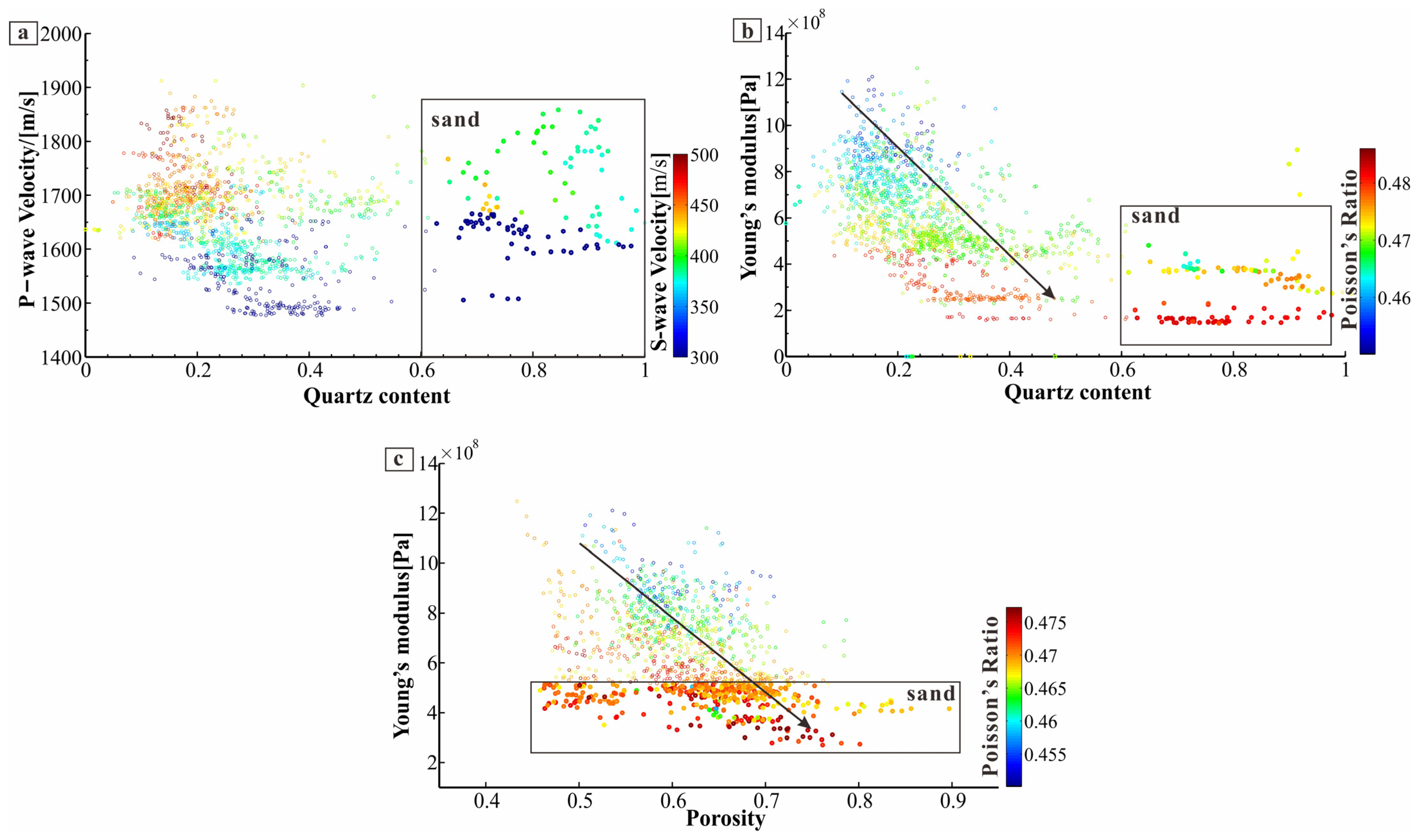
3.1. The Elastic Characteristic of Sandy Sediments

Based on the above model, we change the grain size (0.02 mm~0.1 mm) and quartz content (0~70%) and analyze the effect of grain size and quartz content on Young’s modulus and Poisson’s ratio (Figure 3). The larger the grain size, the smaller Young’s modulus and the larger the Poisson’s ratio. The higher the quartz content, the larger the velocity and the smaller the Poisson’s ratio. This understanding is in line with the conventional understanding, but the shallow marine sands in the South China Sea show some variability.

Well W04 is a well drilled in the Qiongdongnan basin, where several sets of sands were discovered (Figure 4). The sandy layers exhibit lower gamma, lower Young’s modulus, and higher Poisson’s ratio, which are quite different from the elastic characteristics of conventional sands [57].

The Quartz content, derived from logging interpretation, serves as an indicator of sand content. A Quartz content exceeding 60% suggests a sand layer. The P-wave velocity maintains a positive correlation with the S-wave velocity, while the quartz content of the high-velocity layer is low (Figure 5a). The negative correlation between Young’s modulus and quartz content and Poisson’s ratio is obvious (the arrow in Figure 5b). And overall, Young’s modulus is negatively correlated with the porosity (the arrow in Figure 5c). Therefore, the low Young’s modulus and high Poisson’s ratio of the highly porous sand layer contradicts the understanding that the modulus of sand is larger and Poisson’s ratio is smaller than the surrounding clays, since quartz grains are not prone to deformation compared with clay grains, so this feature is not caused by lithology, and there should be other reasons.

In Figure 3, we simply changed the grain size versus quartz content without noticing the relationship between grain size and quartz content. In fact, a suitable relationship between quartz content and grain size should be considered in the model. In this paper, this relationship was obtained by fitting the core data (Figure 6a). Under this relationship, the relationship between quartz content and Young’s modulus and Poisson’s ratio is obtained again based on the above modeling, and as shown in Figure 6b,c, the higher the quartz content, the lower the Young’s modulus and the higher the Poisson’s ratio, which is consistent with the actual logging data. This also verifies the rationality of the above model at the same time.

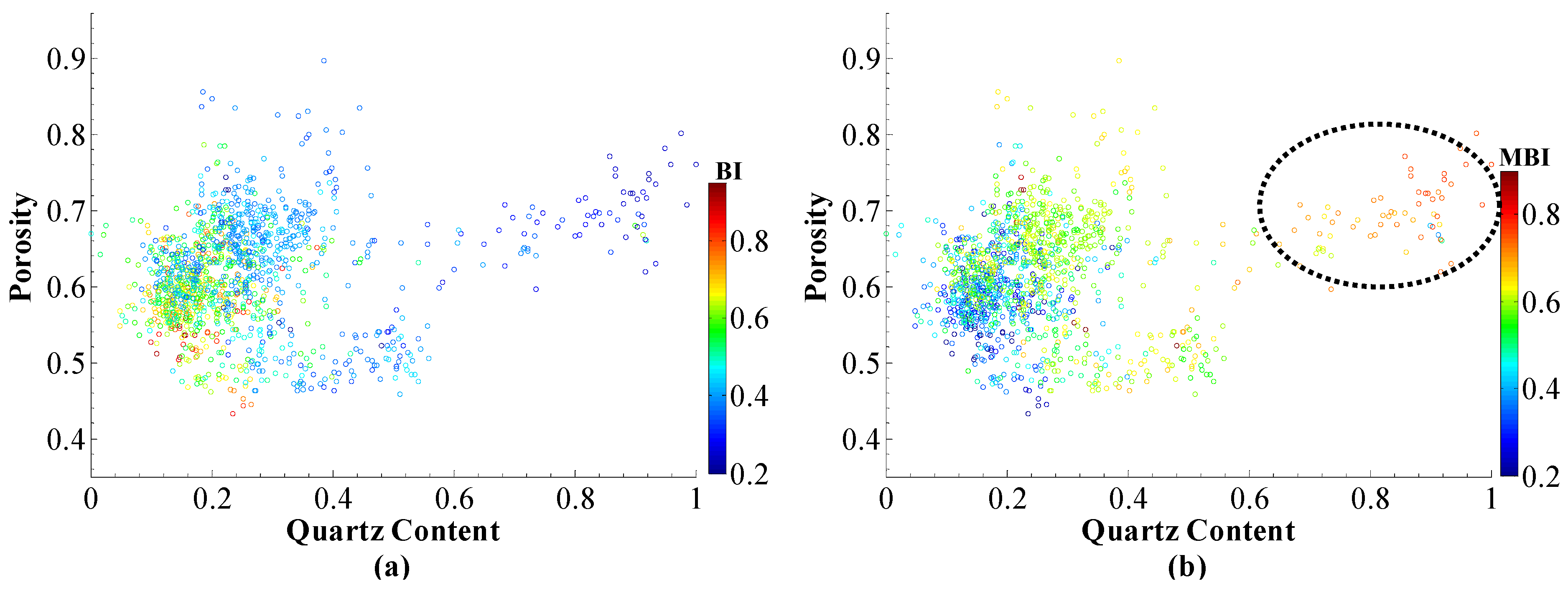
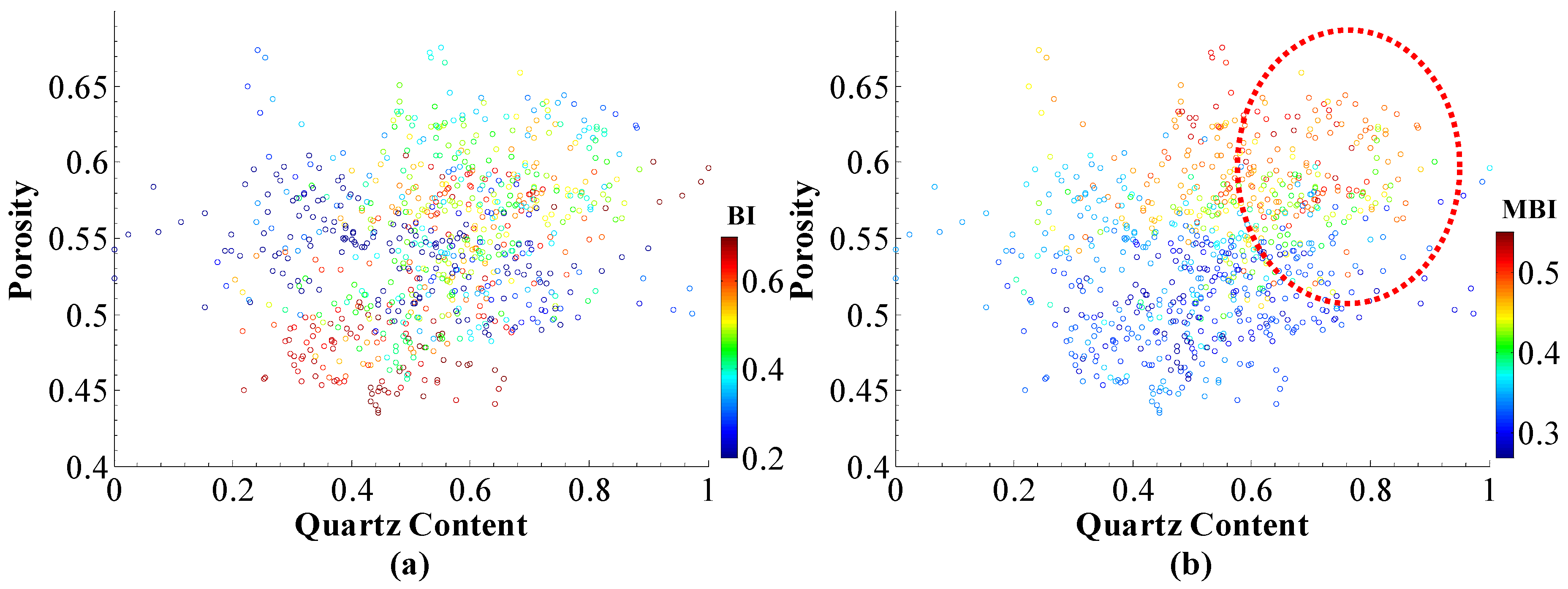
3.2. Elastic Indicator of Sand Content

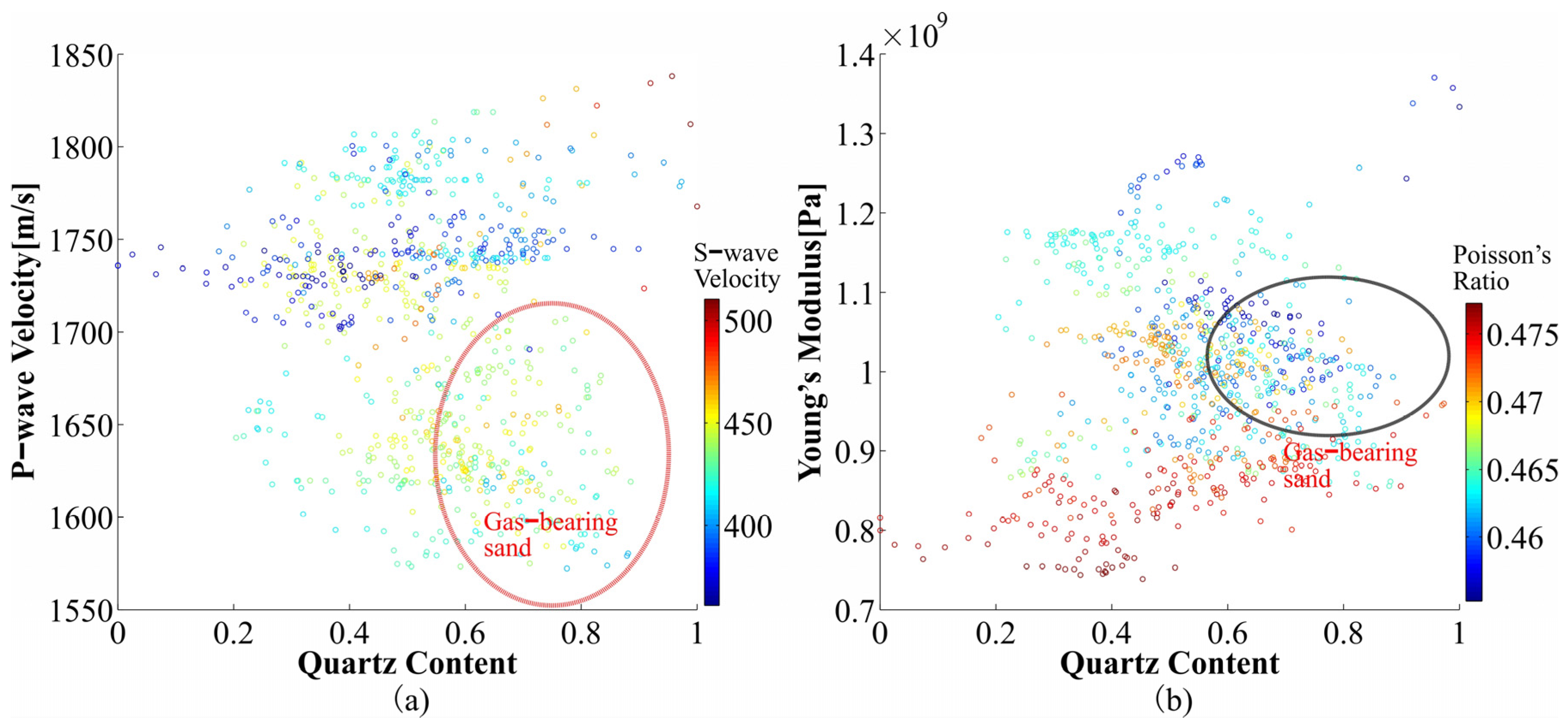
3.2.1. Water Saturated Sandy Sediments

The brittle index (BI) of the rock can be calculated from Young’s modulus and Poisson’s ratio [23], as shown in Equation (17).

$$BI=0.5{\displaystyle \frac{E-E_{\min }}{E_{\max }-E_{\min }}}+0.5{\displaystyle \frac{{\sigma }_{\max }-\sigma }{{\sigma }_{\max }-{\sigma }_{\min }}}$$

(17)

However, the above equation is no longer suitable for the shallow marine sandy sediment in the SCS. Based on the model as well as the analysis of well logging, we newly define a modified brittle index (MBI) and rewritten Equation (17) as Equation (18) in this paper, and MBI is sensitive to the sand content of unconsolidated reservoir.

$$MBI=a{\displaystyle \frac{E_{\max }-E}{E_{\max }-E_{\min }}}+b{\displaystyle \frac{\sigma -{\sigma }_{\min }}{{\sigma }_{\max }-{\sigma }_{\min }}}$$

(18)

where a and b equal to 0.5, generally, but also need to be adjusted according to the real situation. BI and MBI in well W2 were calculated using Equations (17) and (18), and the results are shown in Figure 7. The BI could not identify the sand layers, and the relationship between BI and porosity was not obvious (Figure 7a). However, the MBI well distinguished the high quartz content layer from the low quartz content layer, and in the high quartz content layer section, the MBI was higher, and the porosity was also larger (the circle in Figure 7b). After obtaining Young’s modulus and Poisson’s ratio by seismic inversion, the MBI is calculated according to Equation (18).

3.2.2. Gas-Bearing Sediments

Free gas will have a large effect on Poisson’s ratio; does it affect MBI? A gas-bearing layer was recovered in well W09-2019 [39] in the Qiongdongnan basin (Figure 8). The gas layer is at about 1870~1907 m. The Poisson’s ratio of the gas-bearing layer is obviously reduced, and Young’s modulus is a medium-low value (Figure 9). It can be seen that the section of high MBI still corresponds to the high sand content and high porosity (the red circle in Figure 10). This is because gas occurrence reduces Young’s modulus and Poisson’s ratio, and MBI can offset the effect of gas influence to a certain extent. By adjusting a and b in Equation (18), we can better eliminate the influence of the gas on MBI.

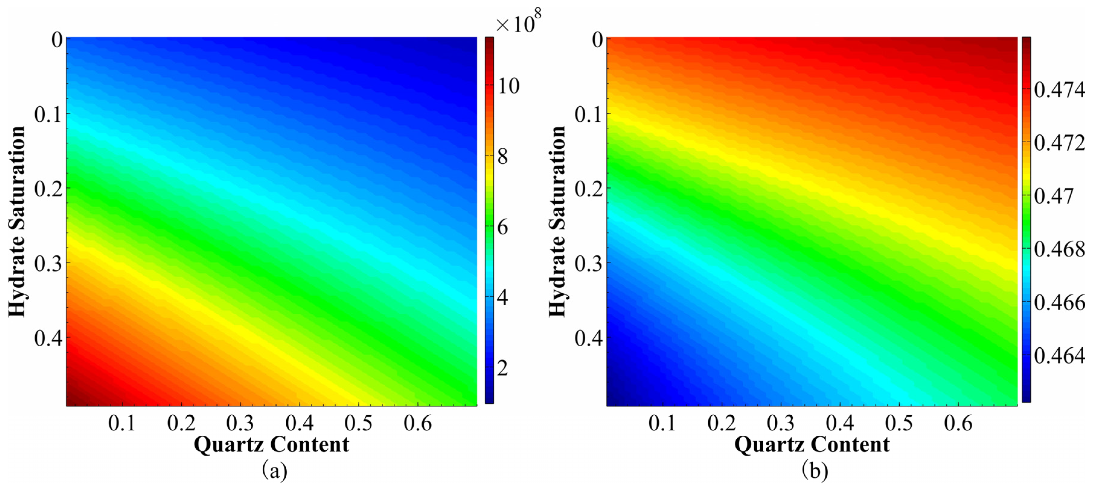
3.2.3. Hydrate-Bearing Sand

Based on the above model, we analyze how hydrate saturation and quartz content influence Young’s modulus and Poisson’s ratio. As shown in Figure 11, Young’s modulus increases, and Poisson’s ratio decreases with increasing hydrate saturation. The change rate of Young’s modulus and Poisson’s ratio caused by hydrate saturation is almost the same, while the change rate caused by quartz content is smaller. Therefore, the MBI of the hydrate layer will be smaller. Assuming that the MBI of water saturated sand is MBI₁, MBI₁ is proportional to the quartz content. Due to the hydrate occurrence, the MBI of the hydrate-bearing sand is reduced to MBI₂, which is almost inversely proportional to the hydrate saturation. Therefore, the hydrate saturation has a greater impact on MBI. If near the bottom of the hydrate layer, the MBI is obviously smaller than the surrounding sediments, which can be used as an indicator of hydrate presence. The smaller the MBI, the higher the hydrate saturation. If the MBI is larger, it indicates that the quartz content has a greater effect on the increase in the MBI than the reduction effect of hydrate saturation, and in this case, the quartz content is high.

A hydrate-bearing sand layer at about 1568~1582 m is discovered in well W01-2019 [31] (Figure 12). The hydrate-bearing sand has a large Young’s modulus and a low Poisson’s ratio. Young’s modulus is proportional to the quartz content (arrow 1 in Figure 13a), and Poisson’s ratio is inversely proportional to the quartz content (arrow 1 in Figure 13b). However, Young’s modulus at the non-hydrate layer and the low-saturation hydrate layer (resistivity 1.5~5 ohm) is low, and Young’s modulus is almost unchanged with the quartz content (arrow 2 in Figure 13a), the Poisson’s ratio increases slightly (arrow 2 in Figure 13b), and the quartz content of this layer is also low.

Therefore, in the hydrate interval, MBI cannot predict well the quartz content. However, in practical applications, we target those formations with high saturation and high sand content, and the MBI in those sections are relatively obvious. According to the results of petrophysical model analysis, if there is a high saturation hydrate (greater than 30%), the MBI decreases significantly. If the hydrate saturation is low, but MBI is large at the same time, it indicates that the quartz content is high.

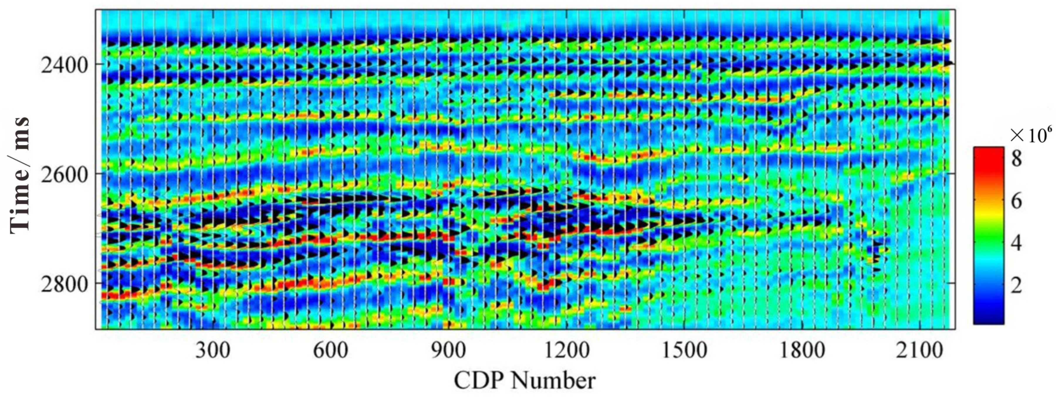
3.3. Seismic Inversion Results

The study area is located in the Lingnan Low uplift in the deep-water area of QDNB [7,47]. The water depth of the study area ranges from 1500 to 1665 m, and the submarine topography is relatively flat. The previous geological survey shows that the many layers of shallow sand is widely distributed. In this paper, one of the seismic lines was selected for actual data testing. Figure 14 shows the overlay display of the post-stack seismic profile and the inverted P-wave impedance. There are obvious amplitude anomalies in the range of 2600 ms~2800 ms at CDP 1~1500, and there are obvious high and low impedance anomalies, which indicate the occurrences of free gas and hydrate in sands.

Recent studies in sedimentology indicate that multi-stage channel-natural levee sedimentary systems are developed in the shallow sediments. Channel systems are identified in the Quaternary strata, and the channel-related sedimentary facies include channel-filling facies, levee facies, crevasse splay facies, and lobes facies [32]. It is suspected that multiple small channels are developed at 2700 ms between CDP 150~1650 (Figure 15), so the sand content is large.

Seismic waves experience varying travel paths, attenuation, and reflection characteristics at different incidence angles, altering the frequency and phase of seismic wavelet. Wide-angle waves encounter stronger formation absorption and dispersion, causing wavelet broadening and frequency attenuation. Thus, amplitude varies in stacked data from different angles. When extracting seismic wavelet, the Aki–Richards equation is used to calculate reflection coefficients at diverse angles using the well logs (P-velocity, S-velocity and density) and then using the well-seismic tie to extract wavelets for each angle. Then, seismic inversion was carried out. Figure 16 shows the inverted MBI, and the MBI are generally high, with anomalies in both the shallow and deep layers. MBI has good lateral continuity and good stratigraphy. MBI can depict more information about mineral composition, which is less affected by other factors. There are certain high sand anomalies in the shallow layer and even on the surface of the seabed, and the anomalies are more obvious in the impedance anomaly area, which may be related to the development of small channels. However, in seismic data, we only notice some anomalies at 2600 ms~2800 ms, but in fact, there are many layers of sand even in the shallower section. Compared with seismic data, MBI inversion has significant advantages in the prediction of sand layers.

4. Discussion

4.1. Effectiveness of MBI

In general, due to the higher density of sandy particles compared to muddy sediment particles, sand layers typically exhibit higher acoustic velocities and produce positive polarity reflections on seismic profiles when their porosity is similar to that of muddy sediments. However, the porosity of shallow sandy sediments may be larger or lower than that of muddy sediments. As shown in Figure 4, the elastic properties of the two sand layers differ significantly, indicating that using only velocity or density parameters is ineffective for identifying sand layers. Figure 17 shows the inversion results for P-wave velocity and density. These results reveal no obvious anomalies in the shallow sand layer, suggesting that P-wave velocity and density parameters alone cannot effectively distinguish shallow sandy sedimentary layers. Previous studies have shown that the study area contains multiple sand bodies from deep to shallow depths, with sand almost throughout the entire area. This is well reflected in the MBI inversion results, which also shows better stratification, further validating the effectiveness of MBI in identifying sand layers.

4.2. Geological Implications

Shallow sands are excellent reservoirs both for shallow gas and gas hydrates, and shallow sandy sediments and their associated hydrocarbon–hydrate systems may be important targets for future offshore exploration and development. The discovery of LS36-1 will significantly accelerate the exploration and development of deep-sea shallow gas and gas hydrate [8]. As the basis for exploring shallow gases and hydrates, identifying shallow sand bodies has been challenging due to insufficient drilling data. Current predictions mostly depend on sedimentary facies interpretation. This study uses actual drilling data from multiple sites in the South China Sea to develop a seismic identification technique for shallow sand layers. It supplements well the existing seismic interpretation methods, effectively predicts the distribution of shallow sand bodies, and offers a qualitative evaluation of their sand content.

The seismic prediction technique proposed in this paper is based on seismic data and leverages pre-stack seismic inversion to derive Young’s modulus and Poisson’s ratio. This method can achieve reliable prediction results even in the absence of well logging data, making it particularly suitable for exploration in new areas [37,61].

Additionally, the elastic properties of shallow sandy sediments differ significantly from those of deeper conventional oil and gas sand reservoirs. However, the study on the elastic characteristics of shallow sands is still weak, which may be attributed to the limited availability of well logging and lithological data for shallow sandy sediments in previous studies. This paper highlights that shallow sands may exhibit varying characteristics at different depths, which are closely related to factors such as effective stress levels and mineral composition. These aspects warrant further in-depth investigation.

5. Conclusions

The properties and elastic characteristics of conventional deep-buried sand layers are well-known. However, the features of shallow unconsolidated sand layers remain poorly understood. Typically, sand layers have high velocity and porosity. Yet, our logging data analysis shows that unconsolidated sand may have high or low velocities, making it hard to identify shallow sand layers using these parameters. In this paper, we focus on the physical properties of the shallow unconsolidated sandy sediments and construct a new petrophysical model to link sand content with elastic parameters, and we derive a new indicator of shallow sand: modified brittleness index (MBI). The theoretical model and the well logs show that MBI has a good indication of quartz content compared with other inversion parameters. Finally, MBI extraction is realized based on pre-stack seismic inversion, and the inversion results are consistent with geological understandings and drilling results. This method can be used in the future shallow gas and hydrate explorations.

This paper offers a solution by developing MBI that incorporates the mechanical properties of shallow sand layers, providing an effective way to identify them. However, this method is only suitable for shallow layers. Also, MBI alone cannot identify hydrate-bearing sand layers. When sediments contain hydrates, their elastic parameters like Young’s modulus and Poisson’s ratio change significantly. In such cases, identification requires both the velocity and MBI. Sandy hydrate-bearing sediments have high velocity and low MBI, while high sand content is indicated by low velocity and low MBI.

References

1. Dickens, G.R.; Quinby, H.M.S. Methane hydrate stability in seawater. Geophys. Res. Lett. 1994, 21, 2115–2118. [Google Scholar] [CrossRef]
2. Kvenvolden, K.A. Methane hydrate a major reservoir of carbon in the shallow geosphere? Chem. Geol. 1988, 71, 41–51. [Google Scholar] [CrossRef]
3. Kvenvolden, K.A. Gas hydrates: Geological perspective and global change. Rev. Geophys. 1993, 31, 173–187. [Google Scholar] [CrossRef]
4. Collett, T.S.; Lee, M.W.; Zyrianova, M.V.; Mrozewski, S.A.; Guerin, G.; Cook, A.E.; Goldberg, D.S. Gulf of Mexico gas hydrate Joint industry Project leg II logging-while-drilling data acquisition and analysis. Mar. Petrol. Geol. 2012, 34, 41–61. [Google Scholar] [CrossRef]
5. Fang, Y.; Flemings, P.B.; Daigle, H.; Phillips, S.; Meazell, K.; You, K. Petrophysical properties of the Green Canyon Block 955 hydrate reservoir inferred from reconstituted sediments: Implications for hydrate formation and production. AAPG Bull. 2020, 104, 1997–2028. [Google Scholar] [CrossRef]
6. Colwell, F.; Matsumoto, R.; Reed, D. A review of the gas hydrates, geology, and biology of the Nankai Trough. Chem. Geol. 2004, 250, 391–404. [Google Scholar] [CrossRef]
7. Kuang, Z.; Cook, A.; Ren, J.; Deng, W.; Cao, Y.; Cai, H. A flat-lying transitional free gas to gas hydrate system in a sand layer in the Qiongdongnan Basin of the South China Sea. Geophys. Res. Lett. 2023, 50, e2023GL105744. [Google Scholar] [CrossRef]
8. Xu, C.; Wu, K.; Pei, J.; Hu, L. Enrichment mechanisms and accumulation model of ultra-deep water and ultra-shallow gas: A case study of Lingshui 36-1 gas field in Qiongdongnan Basin, South China Sea. Pet. Explor. Dev. 2025, 51, 50–63. [Google Scholar] [CrossRef]
9. Ruppel, C. Permafrost-associated gas hydrate: Is it really approximately 1% of the global system? J. Chem. Eng. Data 2015, 60, 429–436. [Google Scholar] [CrossRef]
10. Kessler, J.D.; Ruppel, C.D. Characterizing Ocean Acidification and Atmospheric Emission caused by Methane Released from Gas Hydrate Systems along the US Atlantic Margin (No. DOE-ROCHESTER-0028980); Univeristy of Rochester, Ed.; National Energy Technology Laboratory (NETL): Pittsburgh, PA, USA; Morgantown, WV, USA; Albany, OR, USA, 2020.
11. Farahani, M.V.; Guo, X.; Zhang, L.; Yang, M.; Hassanpouryouzband, A.; Zhao, J.; Yang, J.; Song, Y.; Tohidi, B. Effect of thermal formation/dissociation cycles on the kinetics of formation and pore-scale distribution of methane hydrates in porous media: A magnetic resonance imaging study. Sustain. Energy Fuels 2021, 5, 1567–1583. [Google Scholar] [CrossRef]
12. Farahani, M.V.; Hassanpouryouzband, A.; Yang, J.; Tohidi, B. Insights into the climate-driven evolution of gas hydrate-bearing permafrost sediments: Implications for prediction of environmental impacts and security of energy in cold regions. RSC Adv. 2021, 11, 14334–14346. [Google Scholar] [CrossRef] [PubMed]
13. Maslin, M.; Owen, M.; Day, S.; Long, D. Linking continental-slope failures and climate change: Testing the clathrate gun hypothesis. Geology 2004, 32, 53–56. [Google Scholar] [CrossRef]
14. Meng, M.; Li, L.; Liang, J.; Xu, J.; Feng, J.; Kuang, Z.; Zhang, W.; Huang, W.; Ren, J.; Deng, W.; et al. Quantifying the relative provenance contributions to submarine channel systems in the Qiongdongnan Basin since the Miocene: Implications for tectonic responses and channel migration. Basin Res. 2024, 36, 1365–2117. [Google Scholar]
15. Meng, M.; Liang, J.; Lu, J.A.; Zhang, W.; Kuang, Z.; Fang, Y.; He, Y.; Deng, W.; Huang, W. Quaternary Deep-Water Sedimentary Characteristics and Their Relationship with the Gas Hydrate Accumulations in the Qiongdongnan Basin, Northwest South China Sea. Deep Sea Res. Part I Oceanogr. Res. Pap. 2021, 177, 103628. [Google Scholar] [CrossRef]
16. Yang, Y.; Aplin, A.C. Influence of lithology and compaction on the pore size distribution and modelled permeability of some mudrocks from the Norwegian margin. Mar. Petrol. Geol. 1998, 15, 163–175. [Google Scholar] [CrossRef]
17. Yang, Y.; Aplin, A.C. Definition and practical application of mudstone porosity-effective stress relationships. Petrol. Geosci. 2004, 10, 153–162. [Google Scholar] [CrossRef]
18. Waite, W.F.; Santamarina, J.C.; Cortes, D.D.; Dugan, B.; Espinoza, D.N.; Germaine, J.; Jang, J.; Jung, J.W.; Kneafsey, T.J.; Shin, H.; et al. Physical properties of hydrate-bearing sediments. Rev. Geophys. 2009, 47, RG4003. [Google Scholar] [CrossRef]
19. Harris, N.B.; Miskimins, J.L.; Mnich, C.A. Mechanical anisotropy in the Woodford Shale, Permian Basin: Origin, magnitude, and scale. Lead. Edge 2011, 30, 284–291. [Google Scholar] [CrossRef]
20. Sena, A.; Castillo, G.; Chesser, K.; Voisey, S.; Estrada, J.; Carcuz, J.; Carmona, E.; Schneider, R.V. Seismic reservoir characterization in resource shale plays: “Sweet spot” discrimination and optimization of horizontal well placement. In SEG Technical Program Expanded Abstracts; Society of Exploration Geophysicists: Houston, TX, USA, 2011; p. 4424. [Google Scholar]
21. Mehrabi, A.; Bagheri, M.; Bidhendi, M.N.; Delijani, E.B.; Behnoud, M. Improved porosity estimation in complex carbonate reservoirs using hybrid CRNN deep learning model. Earth Sci. Inf. 2024, 17, 4773–4790. [Google Scholar] [CrossRef]
22. Riahi, Z.T.; Sarkarinejad, K.; Faghih, A.; Soleimany, B.; Payrovian, G.R. Frature detection using multi seismic attributes ant-tracking in the Rag-e-Sefid oilfield, SW Iran. EGU 2024, 21, 12039. [Google Scholar]
23. Rickman, R.; Mullen, M.; Petre, E.; Grieser, B.; Kundert, D. A practical use of shale petrophysics for stimulation design optimization: All shale plays are not clones of the Barnett Shale. In Proceedings of the SPE Annual Technical Conference and Exhibition, Denver, CO, USA, 21–24 September 2008; p. 115258. [Google Scholar]
24. Sondergeld, C.H.; Newsham, K.E.; Comisky, J.T.; Rice, M.C.; Rai, C.S. Petrophysical consideration in evaluation and producing shale gas resources. In Proceedings of the SPE Unconventional Gas Conference, Calgary, AB, Canada, 19–21 October 2010. [Google Scholar]
25. Shelander, D.; Dai, J.; Bunge, G. Predicting saturation of gas hydrates using pre-stack seismic data, Gulf of Mexico. Mar Geophys. Res. 2010, 31, 39–57. [Google Scholar] [CrossRef]
26. Lee, M.W.; Hutchinson, D.R.; Collett, T.S.; Dillon, W.P. Seismic velocities for hydrate-bearing sediments using weighted equation. J. Geophys. Res.-Solid Earth 1996, 101, 20347–20358. [Google Scholar] [CrossRef]
27. Lee, M.W.; Collett, T.S.; Inks, T.L. Seismic-attribute analysis for gas-hydrate and free-gas prospects on the North Slope of Alaska. In Natural Gas Hydrates-Energy Resource Potential and Associated Geologic Hazards; Collett, T., Johnson, A., Knapp, C., Boswell, R., Eds.; AAPG Memoir: Tulsa, OK, USA, 2009; Volume 89, pp. 541–554. [Google Scholar]
28. Waite, W.F.; Helgerud, M.B.; Nur, A.; Pinkston, J.C.; Stern, L.A.; Kirby, S.H.; Durham, W.B. Laboratory measurements of compressional and shear wave speeds through methane hydrate. Ann. N. Y. Acad. Sci. 2000, 912, 1003–1010. [Google Scholar] [CrossRef]
29. Yun, T.S.; Francisca, F.M.; Santamarina, J.C.; Rupple, C. Compressional and shear wave velocities in uncemented sediment containing gas hydrate. Geophys. Res. Lett. 2005, 32, L10669. [Google Scholar] [CrossRef]
30. Dvorkin, J.; Nur, A. Elasticity of high-porosity sandstones: Theory for two North Sea data sets. Geophysics 1996, 61, 1363–1370. [Google Scholar] [CrossRef]
31. Helgerud, M.B.; Dvorkin, J.; Nur, A.; Sakai, A.; Collett, T. Elastic-wave velocity in marine sediments with gas hydrates: Effective medium modeling. Geophys. Res. Lett. 1999, 26, 2021–2024. [Google Scholar] [CrossRef]
32. Lee, M.W. Modifed Biot-Gassmann theory for calculating elastic velocities for unconsolidated and consolidated sediments. Mar. Geophys. Res. 2002, 23, 403–412. [Google Scholar] [CrossRef]
33. Duffaut, K.; Landrø, M.; Sollie, R. Using Mindlin theory to model friction-dependent shear modulus in granular media. Geophysics 2010, 75, E143–E152. [Google Scholar] [CrossRef]
34. Fujii, T.; Saeki, T.; Kobayashi, T.; Inamori, T.; Hayashi, M.; Takano, O.; Takayama, T.; Kawasaki, T.; Nagakubo, S.; Nakamizu, M.; et al. Resource assessment of methane hydrate in the eastern Nankai Trough, Japan. In Proceedings of the Offshore Technology Conference, Houston, TX, USA, 5–8 May 2008; OnePetro: Richardson, TX, USA, 2008. [Google Scholar]
35. Pan, H.; Li, H.; Chen, J.; Zhang, Y.; Cai, S.; Huang, Y.; Zheng, Y.; Zhao, Y.; Deng, J. A unified contact cementation theory for gas hydrate morphology detection and saturation estimation from elastic-wave velocities. Mar. Petrol. Geol. 2020, 113, 104146. [Google Scholar] [CrossRef]
36. Mindlin, R.D. Compliance of elastic bodies in contact. J. Appl. Mech. 1949, 16, 259–268. [Google Scholar] [CrossRef]
37. Zhu, W.; Huang, B.; Mi, L.; Wilkins, R.W.; Fu, N.; Xiao, X. Geochemistry, origin, and deep-water exploration potential of natural gases in the Pearl River Mouth and Qiongdongnan basin, South China Sea. AAPG Bull. 2009, 93, 741–761. [Google Scholar] [CrossRef]
38. Liang, J.; Zhang, W.; Lu, J.A.; Wei, J.; Kuang, Z.; He, Y. Geological occurrence and accumulation mechanism of natural gas hydrates in the eastern Qiongdongnan Basin of the South China Sea: Insights from site GMGS5-W9-2018. Mar. Geol. 2019, 418, 106042. [Google Scholar] [CrossRef]
39. Deng, W.; Kuang, Z.; Liang, J.; Yan, P.; Lu, J.; Meng, M. The seismic and rock-physics evidences of the different migration efficiency between different types of gas chimneys. Deep Sea Res. Part I: Oceanogr. Res. Pap. 2023, 191, 103942. [Google Scholar] [CrossRef]
40. Deng, W.; Liang, J.; Zhang, W.; Kuang, Z.; Zhong, T.; He, Y. Typical characteristics of fracture-filling hydrate-charged reservoirs caused by heterogeneous fluid flow in the Qiongdongnan Basin, northern South China Sea. Mar. Pet. Geol. 2021, 124, 104810. [Google Scholar]
41. Wei, J.; Liang, J.; Lu, J.; Zhang, W.; He, Y. Characteristics and dynamics of gas hydrate systems in the northwestern South China Sea-results of the fifth gas hydrate drilling expedition. Mar. Pet. Geol. 2019, 110, 287–298. [Google Scholar] [CrossRef]
42. Xie, X.; Müller, R.D.; Ren, J.; Jiang, T.; Zhang, C. Stratigraphic architecture and evolution of the continental slope system in offshore Hainan, northern South China Sea. Mar. Geol. 2008, 247, 129–144. [Google Scholar] [CrossRef]
43. Meng, M.; Liang, J.; Kuang, Z.; Ren, J.; He, Y.; Deng, W.; Gong, Y. Distribution characteristics of Quaternary channel systems and their controlling factors in the Qiongdongnan basin, South China Sea. Front. Earth Sci. 2022, 10, 902517. [Google Scholar] [CrossRef]
44. Winkler, K.W. Contact stiffness in granular and porous meterials: Comparison between theory and experiment. Geophys. Res. Lett. 1983, 10, 1073–1076. [Google Scholar] [CrossRef]
45. Walton, K. The effective elastic moduli of a random packing of spheres. J. Mech. Phys. Solids. 1987, 35, 213–226. [Google Scholar] [CrossRef]
46. Dai, S.; Santamarina, J.C.; Waite, W.F.; Kneafsey, T.J. Hydrate morphology: Physical properties of sands with patchy hydrate saturation. J. Geophys. Res. Solid Earth 2012, 117. [Google Scholar] [CrossRef]
47. White, J.E.; Martineau-Nicholetis, L.; Monash, C. Measured anisotropy in Pierre shale. Geophys. Prospect. 1983, 31, 709–729. [Google Scholar] [CrossRef]
48. Backus, G.E. Long-wave elastic anisotropy produced by horizontal layering. J. Geophys. Res. 1962, 67, 4427–4440. [Google Scholar] [CrossRef]
49. Brown, R.; Korringa, J. On the dependence of the elastic properties of a porous rock on the compressibility of the pore fluid. Geophysics 1975, 40, 608–616. [Google Scholar] [CrossRef]
50. Lu, S.; McMechan, G.A. Elastic impedance inversion of multichannel seismic data from unconsolidated sediments containing gas hydrate and free gas. Geophysics 2004, 69, 164–179. [Google Scholar] [CrossRef]
51. Lu, S.; McMechan, G.A.; Liaw, A. Identification of shallow-water-flow sands by Vp/Vs inversion of conventional 3D seismic data. Geophysics 2005, 70, O29–O37. [Google Scholar] [CrossRef]
52. Downton, J.E. Seismic Parameter Estimation from AVO Inversion. Ph.D. Thesis, University of Calgary, Calgary, AB, Canada, 2005. [Google Scholar]
53. Russell, B.H.; Hedlin, K.; Hilterman, F.J.; Lines, L.R. Fluid-property discrimination with AVO: A Biot-Gassmann perspective. Geophysics 2003, 68, 29–39. [Google Scholar] [CrossRef]
54. Russell, B.H.; Gray, D.; Hampson, D.P. Linearized AVO inversion and poroelasticity. Geophysics 2011, 76, C19–C29. [Google Scholar] [CrossRef]
55. Wang, B.; Yin, X.; Zhang, F. Lamé parameters inversion based on elastic impedance and its application. Appl. Geophys. 2006, 3, 120–123. [Google Scholar] [CrossRef]
56. Yin, X.; Zhang, S. Bayesian inversion for effective pore-fluid bulk modulus based on fluid-matrix decoupled amplitude variation with offset approximation. Geophysics 2014, 79, R221–R232. [Google Scholar] [CrossRef]
57. Zong, Z.; Yin, X.; Wu, G. Elastic impedance parameterization and inversion with Young’s modulus and Poisson’s ratio. Geophysics 2012, 77, N17–N24. [Google Scholar] [CrossRef]
58. Zong, Z.; Yin, X.; Wu, G. Geofluid discrimination incorporating poroelasticity and seismic reflection inversion. Surv. Geophys. 2015, 36, 659–681. [Google Scholar] [CrossRef]
59. Aki, K.; Richards, P.G. Quantitative Seismology: Theory and Methods; University Science Books: Herndon, VA, USA, 2002. [Google Scholar]
60. Connolly, P. Elastic impedance. Lead. Edge 1999, 18, 438–452. [Google Scholar] [CrossRef]
61. Shelander, D.; Dai, J.; Bunge, G.; Singh, S.; Eissa, M.; Fisher, K. Estimating saturation of gas hydrates using conventional 3D seismic data, Gulf of Mexico Joint Industry Project Leg II. Mar. Pet. Geol. 2012, 34, 96–110. [Google Scholar] [CrossRef]
Figure 1. The location and channel system in the QDNB. (a) The location of QDNB. The distribution of channel system is from Meng et al. (2021) [15]. (b) The seismic section crossing W01, W03, and W04.
Jmse 13 01044 g001
Figure 2. Schematic diagram of grain contact relations; (a) contact relations of grains with the same size; (b) contact relations of grains with different size. The red dots indicate contact points.
Jmse 13 01044 g002
Figure 3. Effect of grain size and quartz content on Young’s modulus (a) and Poisson’s ratio (b). The color axis is Young’s modulus (a) and Poisson’s ratio (b), respectively.
Jmse 13 01044 g003
Figure 4. Well logs in well W04. The well logs are P-wave velocity, S-wave velocity, Gamma Ray, Porosity, Young’s modulus, and Poisson’s ratio, respectively.
Jmse 13 01044 g004
Figure 5. The crossplot of different parameters. (a) The crossplot of quartz content and P-wave velocity. The color bar is S-wave velocity. (b) the crossplot of quartz content and Young’s modulus; The color bar is Poisson’s ratio. (c) the crossplot of Young’s modulus and porosity. The color bar is Poisson’s ratio.
Jmse 13 01044 g005
Figure 6. Quartz content versus Young’s modulus and Poisson’s ratio after considering the relationship between grain size and quartz content; (a) Grain size versus quartz content. The black dots refer to the cores obtain in the study area; (b) Quartz content versus Young’s modulus; (c) Quartz content versus Poisson’s ratio.
Jmse 13 01044 g006
Figure 7. The crossplots of quartz content and porosity. The color axis is BI (a) and MBI (b).
Jmse 13 01044 g007
Figure 8. Well logs in well W09-2019. The well logs are P-wave velocity, S-wave velocity, Resistivity, Gamma Ray, Porosity, respectively.
Jmse 13 01044 g008
Figure 9. The crossplot of different parameters in well W09-2019. (a) The crossplot of quartz content and P-wave velocity; (b) The crossplot of quartz content and Young’s modulus.
Jmse 13 01044 g009
Figure 10. The crossplots of quartz content and porosity in well W09-2019. The color axis is BI (a) and MBI (b).
Jmse 13 01044 g010
Figure 11. Effect of hydrate saturation and quartz content on Young’s modulus (a) and Poisson’s (b).
Jmse 13 01044 g011
Figure 12. Well logs in well W01-2019. The well logs are P-wave velocity, S-wave velocity, Gamma Ray, Porosity, Young’s modulus, and Poisson’s Ratio, respectively.
Jmse 13 01044 g012
Figure 13. The crossplots of quartz content versus Young’s modulus (a) and Poisson’s ratio (b) in well W3. The color axis is resistivity.
Jmse 13 01044 g013
Figure 14. The overlay display of the post-stack seismic profile and the inverted P-wave impedance.
Jmse 13 01044 g014
Figure 15. Angle stack seismic profiles with different angle ranges. (a) 1~11°; (b) 11~21° (c) 22~35°.
Jmse 13 01044 g015
Figure 16. The inverted MBI profile.
Jmse 13 01044 g016
Figure 17. The inverted P-wave velocity (a) and density (b).
Jmse 13 01044 g017