Position Calibration Technology for Long-Term Endurance Inertial Navigation Systems Based on Sparse and Low-Precision Position Information

Abstract

To enhance the long-term endurance navigation and positioning capabilities of inertial navigation systems (INSs), external auxiliary information is typically required for calibration. However, in certain challenging environments, obtaining continuous reliable and high-precision auxiliary information becomes difficult, and only sparse and low-precision position information may be available. Investigating methods to utilize this unfavorable information for calibrating INSs holds significant practical value. Building upon the inherent error characteristics of INSs, this study introduces a novel position calibration methodology. The first step is to make a comprehensive judgment by combining the position calculated by the INS and the reference position and selecting the usable sparse and low-precision reference position that meets the judgment conditions. The second step is to calibrate the INS with reference positions that meet the judgment conditions. Finally, a simulation static test and dynamic test were carried out; in the simulation static test, the std value of the latitude error decreased from 0.3250 $\mathrm{n} \mathrm{mile}$ to 0.2245 $\mathrm{n} \mathrm{mile}$, and the accuracy improved by 30.92%; the max value of the longitude error decreased from 8.2168 $\mathrm{n} \mathrm{mile}$ to 1.1629 $\mathrm{n} \mathrm{mile}$, and the accuracy improved by 85.85%; and the max value of the position error decreased from 8.2168 $\mathrm{n} \mathrm{mile}$ to 1.2003 $\mathrm{n} \mathrm{mile}$, and the accuracy improved by 85.39%. In the simulation dynamic test, the std value of the latitude error decreased from 0.4501 $\mathrm{n} \mathrm{mile}$ to 0.2384 $\mathrm{n} \mathrm{mile}$, and the accuracy improved by 47.03%; the max value of the longitude error decreased from 3.5907 $\mathrm{n} \mathrm{mile}$ to 0.9383 $\mathrm{n} \mathrm{mile}$, and the accuracy improved by 73.87%; and the max value of the position error decreased from 3.5931 $\mathrm{n} \mathrm{mile}$ to 1.0581 $\mathrm{n} \mathrm{mile}$, and the accuracy improved by 70.55%. The results of these tests show that the cumulative error which grows with time in INSs is obviously suppressed.

1. Introduction

Inertial navigation systems (INSs) have been widely used in military and civil fields; with the development of science and technology, INSs play important roles in space, aviation, marine, and other scenarios [1,2,3]. The advantage of INSs is that they have autonomy and covertness and can provide the carrier’s comprehensive information, such as attitude, velocity, and position, without transmitting and receiving signals [4]. However, it has its own shortcomings, and INS errors accumulate over time, which presents serious challenges to the application of long-term endurance navigation and positioning.

To fully utilize the advantages of the INS and avoid its shortcomings, other reference information is generally needed to assist in suppressing the INS cumulative error. The final effect is closely related to the accuracy of the reference information [1]. The global navigation satellite system (GNSS) is the most common type of navigation and positioning system and has the function of timing. GNSS/INS integrated navigation systems are popular research topics and have been widely studied [5,6,7,8,9]. However, in some special environments, reference information is not easy to obtain, the accuracy of the reference information is relatively low, and the continuity is poor. For example, GNSS signals cannot be received in underwater environments, so the GNSS/INS will fail. Acoustic positioning systems (APSs) are available underwater with relatively high accuracy, but the premise of APSs requires the installation of base stations, which is costly and difficult and is a local positioning method [10,11]. The gravity-assisted inertial navigation system (GAINS) is an important method for underwater autonomous passive navigation and positioning [12]; however, the accuracy of the gravity database affects the accuracy of matching [13]. If only the gravity database obtained from the inversion of satellite altimetry data is used for matching, the accuracy of reference position information obtained through matching is limited [13]. Moreover, in some regions within the global sea area where gravity changes are not obvious, it is difficult to obtain an effective matching position when passing through these regions, and the continuity and stability of gravity matching are difficult to guarantee [14]. For application scenarios on the water surface, the GNSS can provide reference information, but satellite signals are vulnerable to spoofing and interference, which limit its application [15,16,17]. At this point, the celestial navigation system (CNS) provides an optional solution; if the CNS/INS integrated navigation method is adopted, a good observation environment needs to be ensured, such as clear weather and no cloud cover; otherwise, the continuity of the CNS is also difficult to guarantee, and the positioning accuracy is limited [18,19].

In practical applications, if continuous, stable, and high-precision location information can be obtained, such as using the GNSS in an ideal environment, the GNSS/INS based on the Kalman filtering (KF) algorithm is a very classic integrated navigation mode. However, this is not the focus of discussion in this manuscript. The issue of how to calibrate INSs using sparse and low-precision position information can roughly be divided into two categories: one is the integrated navigation mode based on KF [20], or improved formal KF, such as extended KF (EKF) [21,22], unscented Kalman filtering (UKF) [23,24], etc., and the other is comprehensive calibration, such as two-point calibration [25,26,27] and three-point calibration [28]. For the integrated navigation mode, first of all, since the external auxiliary positions are sparse and of a low precision, this means that the frequency of measurement updates using KF will be very low. At the same time, driven by system noise, only time updates are carried out, and the estimated value accuracy of KF will gradually decrease. Secondly, only one external auxiliary position is obtained at a time, which lacks sufficient convergence time for KF. Furthermore, low-precision position measurement can also affect the accuracy of the state estimation values. For comprehensive calibration, as the name suggests, two-point calibration requires two measurements of information, generally including position and yaw angle. However, the yaw angle usually comes from the CNS, which is not easy to obtain in practical applications. Three-point calibration requires three measurement pieces of information, and only the position is needed. However, it cannot guarantee that the position information can be obtained at every ideal moment when calibration is required, and there is a lack of effective judgment on the availability of position information. Moreover, there are certain requirements for the time interval between two adjacent measurement pieces of information in three-point calibration. These limitations increase the difficulty of implementation.

In some special circumstances, although continuous, stable, and high-precision position reference information is expected to be obtained, it is actually very difficult, and only sparse and low-precision position information can be obtained from time to time; this information is still useful auxiliary information in INS long-term endurance navigation applications. The key lies in how to use it. Therefore, it is necessary to study INS position calibration on the basis of sparse and low-precision position information.

Based on the above analysis, in order to enhance the long-endurance navigation and positioning capability of INSs, a new comprehensive judgment method is proposed in this paper. This method combines the INS position and the external auxiliary position for real-time comprehensive judgments. Once the external auxiliary position meets the judgment conditions, it is used for the INS position calibration. This comprehensive judgment method is implemented based on the INS error law. In comparison, the method proposed in this paper is simple and feasible, with basically no constraints. As long as the external auxiliary positions meet the judgment conditions, comprehensive calibration can be carried out. The simulation static test and dynamic test results prove the effectiveness of the method.

A method is proposed in this paper to calibrate INS based on sparse and low-precision position information, and this method has important application value. For the interpretation of the “sparse” feature, in reality, when the measurement information can be obtained and the time interval between two adjacent information measurements are uncertain, it could be several minutes or several hours apart. In the common GNSS/INS integrated navigation mode, the frequency of GNSS data is generally 1 hz, that is, the time interval is 1 s. The main feature of sparsity is large and uneven time intervals, which is significantly different from the situation in GNSSs. During the application process, it is necessary to monitor in real time whether there is a signal transmission in the signal channel, such as through a serial port, which can be achieved by setting flags. For the interpretation of the “low-precision” feature, in reality, a reference position is obtained, but its precision is unknown. The position error is in the order of hundreds of meters or even larger. If these reference positions are used without any judgment, it may not only fail to improve the navigation and positioning accuracy, but also reduce it. Therefore, it is necessary to set judgment conditions to determine whether this reference position is available. In the absence of a true value, only the INS position and the reference position are available. Therefore, a comprehensive judgment is made by combining the INS position and the reference position at adjacent times. As can be seen from the above, we have almost no constraints on the reference position. Therefore, the reliance on continuous and high-precision auxiliary information is reduced.

The content of this paper is arranged as follows, Section 1 introduces the research background and significance, and Section 2 introduces the INS update calculation and error law. Section 3 introduces the position calibration method, and the test verification is shown in Section 4, in which the simulation static test and dynamic test designs are provided. Section 5 presents the conclusion, and Section 6 presents the discussion.

2. INS Update Calculation and Error Law

2.1. INS Update Calculation

The description of the carrier’s movement is carried out in a specific space and is represented by a coordinate system. Among them, the measured values of INSs are relative to the inertial system. The navigation parameters of the carrier are most commonly represented in the navigation coordinate system. Meanwhile, in the process of INS update calculation, the mutual conversion between different coordinate systems is involved. The following is a brief introduction to different coordinate systems.

Inertial coordinate system ($i$-frame): represented by $o{x}_i{y}_i{z}_i$, the coordinate origin is at the center of the Earth, the $o{x}_i$ axis points to the vernal equinox, the $o{z}_i$ axis is the Earth’s rotation axis, pointing to the north pole, and the $o{y}_i$ axis is within the Earth’s equatorial plane, forming a right-handed rectangular coordinate system with the $o{x}_i$ axis and the $o{z}_i$ axis.

Earth coordinate system ($e$-frame): represented by $o{x}_e{y}_e{z}_e$, the origin of the coordinate system is at the center of the Earth. The $o{x}_e$ axis points to the prime meridian, and the $o{z}_e$ axis is the Earth’s axis of rotation, pointing to the north pole. The $o{y}_e$ axis, along with the $o{x}_e$ axis and the $o{z}_e$ axis, forms a right-handed rectangular coordinate system. The $e$-frame is fixedly connected to the Earth and is also known as the Earth-centered earth-fixed (ECEF) frame.

Geographic coordinate system ($g$-frame): represented by $o{x}_g{y}_g{z}_g$, the coordinate origin is at the center of the carrier. The $o{x}_g$ axis points east along the prime vertical circle, the $o{y}_g$ axis points north along the meridian circle, and the $o{z}_g$ axis points upward along the normal of the ellipsoid. This is also a right-handed rectangular coordinate system.

Navigation coordinate system ($n$-frame): represented by $o{x}_n{y}_n{z}_n$, the coordinate origin is at the center of the carrier. The $o{x}_n$ axis points to the geographical east, the $o{y}_n$ axis points to the geographical north, and the $o{z}_n$ axis is perpendicular to the ellipsoid and points upwards, forming the common east–north–up (ENU) coordinate system.

Body coordinate system ($b$-frame): represented by $o{x}_b{y}_b{z}_b$, the coordinate origin is at the center of the carrier. The $o{x}_b$ axis points to the right, the $o{y}_b$ axis points forward, and the $o{z}_b$ axis points upward. The $b$-frame is fixedly connected to the carrier.

The INS is realized on the basis of Newton’s law of motion, and its solution involves the transformation of the coordinate system [29]. For details, please refer to [4]. The navigation results are shown here in the most commonly used navigation frame ($n$ frame), which is a kind of Cartesian coordinate system, and $x$, $y$, and $z$ correspond to east, north, and upward, respectively [30].

The core components of INSs are gyroscopes and accelerometers, which measure angular velocity and acceleration information, respectively, to obtain navigation parameters such as the attitude velocity and position [29]. The attitude update equation of INS is as follows:

$$\stackrel{·}{C_b^n}=C_b^n\left({\omega }_{nb}^b\times \right)$$

(1)

where $C_b^n$ is the direction cosine matrix, which contains the attitude information of the carrier; the dot · above the letter represents the differential, $\stackrel{·}{C_b^n}$ represents the differential of $C_b^n$, ${\omega }_{nb}^b\times$ is the antisymmetric matrix of ${\omega }_{nb}^b$, and ${\omega }_{nb}^b$ represents the projection of the rotational angular velocity of the $b$ frame with respect to the $n$ frame under the $b$ frame. The asymmetric matrix is a mathematical representation for $V={\left[\begin{array}{ccc}{V}_x& V_y& V_z\end{array}\right]}^T$, which has the following antisymmetric matrix:

$$V\times =\left[\begin{array}{ccc}0& -V_z& V_y\\ V_z& 0& -V_x\\ -V_y& V_x& 0\end{array}\right]$$

(2)

$${\omega }_{nb}^b={\omega }_{ib}^b-C_n^b{\omega }_{in}^n$$

(3)

$${\omega }_{in}^n={\omega }_{ie}^n+{\omega }_{en}^n$$

(4)

where the superscript $T$ stands for transpose, ${\omega }_{ib}^b$ is the observed value of the gyroscope, representing the projection of the rotational angular velocity of the $b$ frame relative to the $i$ frame on the $b$ frame, ${\omega }_{in}^n$ represents the projection of the rotational angular velocity of the $n$-frame with respect to the $i$-frame on the $n$-frame, ${\omega }_{ie}^n$ represents the projection of the Earth’s rotational angular velocity in the $n$ frame, and ${\omega }_{en}^n$ represents the projection of the rotational angular velocity of the $n$ frame with respect to the $e$ frame on the $n$ frame.

$${\omega }_{ie}^n={\left[\begin{array}{ccc}0& {\omega }_{ie}\cos L& {\omega }_{ie}\sin L\end{array}\right]}^T$$

(5)

$${\omega }_{en}^n={\left[\begin{array}{ccc}{\displaystyle \frac{-v_N}{R_M+h}}& {\displaystyle \frac{v_E}{R_N+h}}& {\displaystyle \frac{v_E}{R_N+h}}\tan L\end{array}\right]}^T$$

(6)

where ${\omega }_{ie}$ represents the angular velocity of the Earth’s rotation, $L$ represents the latitude, $R_M$ represents the meridian curvature radius, $R_N$ represents the normal radius of the ellipsoid, $h$ represents the Earth’s height, and $v_E$ and $v_N$ represent the east and north velocities, respectively.

The velocity update equation is as follows:

$$\stackrel{·}{v_{en}^n}=C_b^n{f}^b-\left(2{\omega }_{ie}^n+{\omega }_{en}^n\right)\times v_{en}^n+g^n$$

(7)

where $v_{en}^n$ represents the velocity; $\stackrel{·}{v_{en}^n}$ represents the differential of $v_{en}^n$; $f^b$ denotes the specific force corresponding to the observed value of the accelerometer; and $g^n$ is the acceleration of gravity.

The position update equation is as follows:

$$\begin{array}{l}\stackrel{·}{L}={\displaystyle \frac{v_N}{R_M+h}}\\ \stackrel{·}{\lambda }={\displaystyle \frac{v_E}{R_N+h}}\sec L\\ \stackrel{·}{h}=v_{\mathrm{U}}\end{array}$$

(8)

where $\stackrel{·}{L}$ represents the differential of $L$; $\lambda$ represents the longitude; $\stackrel{·}{\lambda }$ represents the differential of $\lambda$; $\stackrel{·}{h}$ represents the differential of $h$; and $v_{\mathrm{U}}$ represents the velocity up component. Notably, the INS up direction is divergent, and it is usually compensated by information provided by other equipment [31]; moreover, setting it to a fixed value in the scene where the height does not change significantly is feasible. Therefore, only the horizontal direction is considered in this paper.

2.2. INS Error Law

An analysis of the INS static error equations reveals that the characteristic roots are all imaginary, the characteristic root is a complex number, and the real parts are all zero, which indicates that the pure INS is a critically stabilized system. There are three periodical oscillation angular frequencies in the navigational solution, which are ${\omega }_{ie}$, ${\omega }_s-{\omega }_f$, and ${\omega }_s+{\omega }_f$, respectively; ${\omega }_{ie}$ is the Earth oscillation angular frequency; ${\omega }_s$ is the Schuler oscillation angular frequency; and ${\omega }_f$ is the Foucault oscillation angular frequency.

By ignoring the Foucault oscillation term, the INS latitude error equation can be expressed as

$$\delta L=A{\epsilon }_E+B{\epsilon }_N+C{\epsilon }_U+D;$$

(9)

among them,

$$A={\displaystyle \frac{{{\omega }_s}^2}{{{\omega }_s}^2-{{\omega }_{ie}}^2}}\left({\displaystyle \frac{\sin {\omega }_{ie}t}{{\omega }_{ie}}}-{\displaystyle \frac{\sin {\omega }_{s}t}{{\omega }_s}}\right)$$

(10)

$$B={\displaystyle \frac{{\omega }_{ie}\sin L}{{{\omega }_s}^2-{{\omega }_{ie}}^2}}\left(\cos {\omega }_{s}t-{\displaystyle \frac{{{\omega }_s}^2}{{{\omega }_{ie}}^2}}\cos {\omega }_{ie}t\right)+{\displaystyle \frac{\sin L}{{\omega }_{ie}}}$$

(11)

$$C={\displaystyle \frac{{{\omega }_s}^2\cos L}{{\omega }_{ie}\left({{\omega }_s}^2-{{\omega }_{ie}}^2\right)}}\cos {\omega }_{ie}t-{\displaystyle \frac{{\omega }_{ie}\cos L}{\left({{\omega }_s}^2-{{\omega }_{ie}}^2\right)}}\cos {\omega }_{s}t-{\displaystyle \frac{\cos L}{{\omega }_{ie}}}$$

(12)

$$D={\displaystyle \frac{{\nabla }_N}{g}}\left(1-\cos {\omega }_{s}t\right).$$

(13)

The longitude error equation can be expressed as

$$\delta \lambda =E{\epsilon }_E+F{\epsilon }_N+G{\epsilon }_U+H;$$

(14)

among them,

$$E={\displaystyle \frac{\tan L}{{\omega }_{ie}}}\left(1-\cos {\omega }_{ie}t\right)-{\displaystyle \frac{{\omega }_{ie}\tan L}{{{\omega }_s}^2-{{\omega }_{ie}}^2}}\left(\cos {\omega }_{ie}t-\cos {\omega }_{s}t\right)$$

(15)

$$F={\displaystyle \frac{{{\omega }_s}^2-{{\omega }_{ie}}^2{\cos }^{2}L}{{\omega }_s\left({{\omega }_s}^2-{{\omega }_{ie}}^2\right)\cos L}}\sin {\omega }_{s}t-{\displaystyle \frac{{{\omega }_s}^2\tan L\sin L}{{\omega }_{ie}\left({{\omega }_s}^2-{{\omega }_{ie}}^2\right)}}\sin {\omega }_{ie}t-t\cos L$$

(16)

$$G={\displaystyle \frac{{{\omega }_s}^2\sin L}{{\omega }_{ie}\left({{\omega }_s}^2+{{\omega }_{ie}}^2\right)}}\sin {\omega }_{ie}t-{\displaystyle \frac{{{\omega }_{ie}}^2\sin L}{{\omega }_s\left({{\omega }_s}^2+{{\omega }_{ie}}^2\right)}}\sin {\omega }_{s}t-t\sin L$$

(17)

$$H={\displaystyle \frac{{\nabla }_E}{g\cos L}}\left(1-\cos {\omega }_{s}t\right).$$

(18)

Furthermore, by removing the Schuler oscillation and Earth oscillation terms from the error equations, the error equations simplify to the following:

$$\delta L={\displaystyle \frac{\sin L}{{\omega }_{ie}}}{\epsilon }_N-{\displaystyle \frac{\cos L}{{\omega }_{ie}}}{\epsilon }_U+{\displaystyle \frac{{\nabla }_N}{g}}$$

(19)

$$\delta \lambda ={\displaystyle \frac{\tan L}{{\omega }_{ie}}}{\epsilon }_E-t\cos L{\epsilon }_N-t\sin L{\epsilon }_U+{\displaystyle \frac{{\nabla }_E}{g\cos L}}.$$

(20)

The INS error equation shows that the latitude error is characterized mainly by oscillation around a constant value, and the longitude error has not only an oscillation term but also an increasing trend term with time, which is unbounded theoretically. In addition, because the inertial device error is difficult to eliminate completely, the oscillation amplitude becomes increasingly larger because of random errors.

3. Position Calibration Method

After the INS works properly, the attitude, velocity, and position information of the carrier can be obtained continuously. This paper focuses on how to make use of the sparse and low-precision position reference information obtained to suppress the INS positioning error.

One of the core steps of this process is to judge the reference position information, that is, to determine whether the reference position information is available. Obviously, if the reference information is not available and is incorrectly applied to INS calibration, it will not only improve the navigation positioning accuracy but also play the opposite role. The process of determining the reference position is described next; for the reference latitude, the difference between the reference latitude and the INS latitude at time $k-1$ is as follows:

$$La{t}_{err1}=La{t}_{Reference}(k-1)-La{t}_{INS}(k-1).$$

(21)

The difference between the reference latitude and the INS latitude at time $k$ is as follows:

$$La{t}_{err2}=La{t}_{Reference}(k)-La{t}_{INS}(k).$$

(22)

The difference between the reference latitude at time $k$ and time $k-1$ is as follows:

$$La{t}_{err3}=La{t}_{Reference}(k)-La{t}_{Reference}(k-1).$$

(23)

The difference between the INS latitude at time $k$ and the reference latitude at time $k-1$ is as follows:

$$La{t}_{err4}=La{t}_{INS}(k)-La{t}_{Reference}(k-1).$$

(24)

If condition 1,

$$La{t}_{err1}>0 and La{t}_{err2}>0 and \left|La{t}_{err3}\right|<\left|La{t}_{err4}\right|,$$

(25)

or condition 2,

$$La{t}_{err1}<0 and La{t}_{err2}<0 and \left|La{t}_{err3}\right|<\left|La{t}_{err4}\right|,$$

(26)

is met, the reference latitude at time $k$ is available.

A further explanation is as follows: the validity of Equation (25) means that the reference latitude is between the true latitude and the INS latitude and is smaller than the true latitude but larger than the INS latitude. Taking the reference latitude at time $k-1$ as the benchmark, the variation range of the reference latitude at two adjacent times (time $k-1$ and time $k$) is smaller than that of the INS latitude. The validity of Equation (26) means that the reference latitude is between the true latitude and the INS latitude and is larger than the true latitude but smaller than the INS latitude. Taking the reference latitude at time $k-1$ as the benchmark, the variation range of the reference latitude at two adjacent times (time $k-1$ and time $k$) is smaller than that of the INS latitude.

For the reference longitude, the difference between the reference longitude and the INS longitude at time $k-1$ is as follows:

$$Lo{n}_{err1}=Lo{n}_{Reference}(k-1)-Lo{n}_{INS}(k-1).$$

(27)

The difference between the reference longitude and the INS longitude at time $k$ is as follows:

$$Lo{n}_{err2}=Lo{n}_{Reference}(k)-Lo{n}_{INS}(k).$$

(28)

The difference between the reference longitude at time $k$ and time $k-1$ is as follows:

$$Lo{n}_{err3}=Lo{n}_{Reference}(k)-Lo{n}_{Reference}(k-1).$$

(29)

The difference between the INS longitude at time $k$ and time $k-1$ is as follows:

$$Lo{n}_{err4}=Lo{n}_{INS}(k)-Lo{n}_{INS}(k-1).$$

(30)

If condition 1,

$$Lo{n}_{err1}>0 and Lo{n}_{err2}>0 and \left|Lo{n}_{err3}\right|<\left|Lo{n}_{err4}\right|,$$

(31)

or condition 2,

$$Lo{n}_{err1}<0 and Lo{n}_{err2}<0 and \left|Lo{n}_{err3}\right|<\left|Lo{n}_{err4}\right|,$$

(32)

is met, the reference longitude at time $k$ is available.

A further explanation is as follows: the validity of Equation (31) means that the reference longitude is between the true longitude and the INS longitude and is smaller than the true longitude but larger than the INS longitude. The variation range of the reference longitude at two adjacent times (time $k-1$ and time $k$) is smaller than that of the INS longitude. The validity of Equation (32) means that the reference longitude is between the true longitude and the INS longitude and is larger than the true longitude but smaller than the INS longitude. The variation range of the reference longitude at two adjacent times (time $k-1$ and time $k$) is smaller than that of the INS longitude.

Overall, the judgment conditions are set based on the INS error law. Suppose there is a true value. Through analysis, it can be known that the INS latitude oscillates around the true latitude. The INS longitude also oscillates relative to the true longitude; meanwhile, as the error accumulates over time, it will gradually deviate from the true value. Obviously, for latitude, the greater the amplitude of oscillation, the greater the error. For longitude, it is somewhat special. As time goes by, the influence of a cumulative error will exceed that of an oscillation error. Therefore, the farther the deviation, the greater the error.

As for why the INS position and reference position at two adjacent moments are compared, the main reason is that in practical applications, there is a lack of true values, thus making it impossible to determine the accuracy of the reference position. However, the difference between two adjacent moments can serve as an effective reference quantity.

Here, the reference latitude and longitude are judged separately, and it should be noted that there is no order of a precedence constraint for judging the reference latitude and longitude. After the judgment of the reference position is completed, INS position calibration can be started. Here, the reference position meeting the judgment condition is directly assigned to the INS position. Notably, the reference latitude and longitude are carried out separately in the judgment process, and the same process is conducted separately in the position calibration. The steps are as follows: judge whether the reference latitude meets the requirement; if it meets the requirement, calibrate it; if not, skip the calibration and go to the next judgment. Judge whether the reference longitude meets the requirement; if it meets the requirement, then calibrate it; if not, skip the calibration and go to the next judgment. The pseudo-code is shown in Algorithm 1.

Algorithm 1: INS calibration technology

Input: INS position and reference position at time $k$ and $k-1$

Output: INS position after calibration

1   Begin:

2     step1: Determine if the reference latitude meets the requirements

3     If the requirement is met

4      step2: The reference latitude calibrates the INS latitude

5     If the requirement is not met

6      step3: Skip this calibration to the next judgment.

7     step4: Determine if the reference longitude meets the requirements

8     If the requirement is met

9      step5: The reference longitude calibrates the INS longitude

10   If the requirement is not met

11     step6: Skip this calibration to the next judgment.

12   end

Based on the above process, the comprehensive calibration of INSs using sparse and low-precision position information has been theoretically achieved. Next comes the testing part.

4. Test Verification

To verify the method developed in this paper, simulation tests are carried out, which are divided into static and dynamic parts.

4.1. Simulation Static Test

In the static simulation test, the position of the carrier is 34.368683° N, 109.221731° E, the height is 0, and the simulation duration is 5 days. The error of the inertial device is shown in

Table 1. Inertial device accuracy.

Inertial Device Error	Value
Gyroscope drifts	0.001 °/h
Accelerometer drifts	10 ug
Gyroscope angular random walk	0.0001 °/h
Accelerometer velocity random walk	1 $\mathrm{ug}/\sqrt{\mathrm{hz}}$

, and the initial error setting is shown in

Table 2. INS initial error setting.

INS Initial Error	Value
Pitch angle error	−6 ″
Roll angle error	6 ″
Yaw angle error	0.3 ′
East velocity error	0.01 m/s
North velocity error	0.01 m/s
Upward velocity error	0.01 m/s
Latitude error	10 m
Longitude error	10 m
Height error	10 m

.

The reference position is generated by adding a random value ranging from −400 to 400 m to the actual position. In the test, a reference position is set to be obtained every 2 h. At the same time, a label of 0 or 1 is randomly generated, where 0 means that the currently obtained reference position is unavailable and where 1 means that the currently obtained reference position is available. This is more realistic, and in reality, there is no guarantee that a reference position will always be available at 2 h intervals.

A further explanation is that 60 reference positions can theoretically be obtained within the simulation time of 5 days, and the label of the corresponding moment is 1, which proves that the reference position is indeed obtained at the current moment. By setting a random label of 0 or 1, the number of reference positions actually obtained will be less than or equal to 60. On this basis, the reference position of the corresponding moment with label 1 is further comprehensively judged, and position calibration is carried out if the judgment conditions are met. In fact, this condition is relatively strict; generally, the positioning results given by common positioning systems have a certain degree of continuity. In the test, the reference positions are represented by the generated random numbers with obvious jumps, which can more favorably illustrate the effectiveness of the algorithm.

For the medium–high-precision INSs, the error accumulation is limited to a short period of time, calibration is not required in this stage, and the calibration is set to start after the 12th h in the simulation test. Next, the test results are discussed; moreover, to conduct a quantitative analysis of the results, the maximum value and standard deviation are calculated, expressed as max and std values, respectively. In addition, considering that the error has positive and negative values, the absolute value of the error is calculated first, and then the max value is obtained.

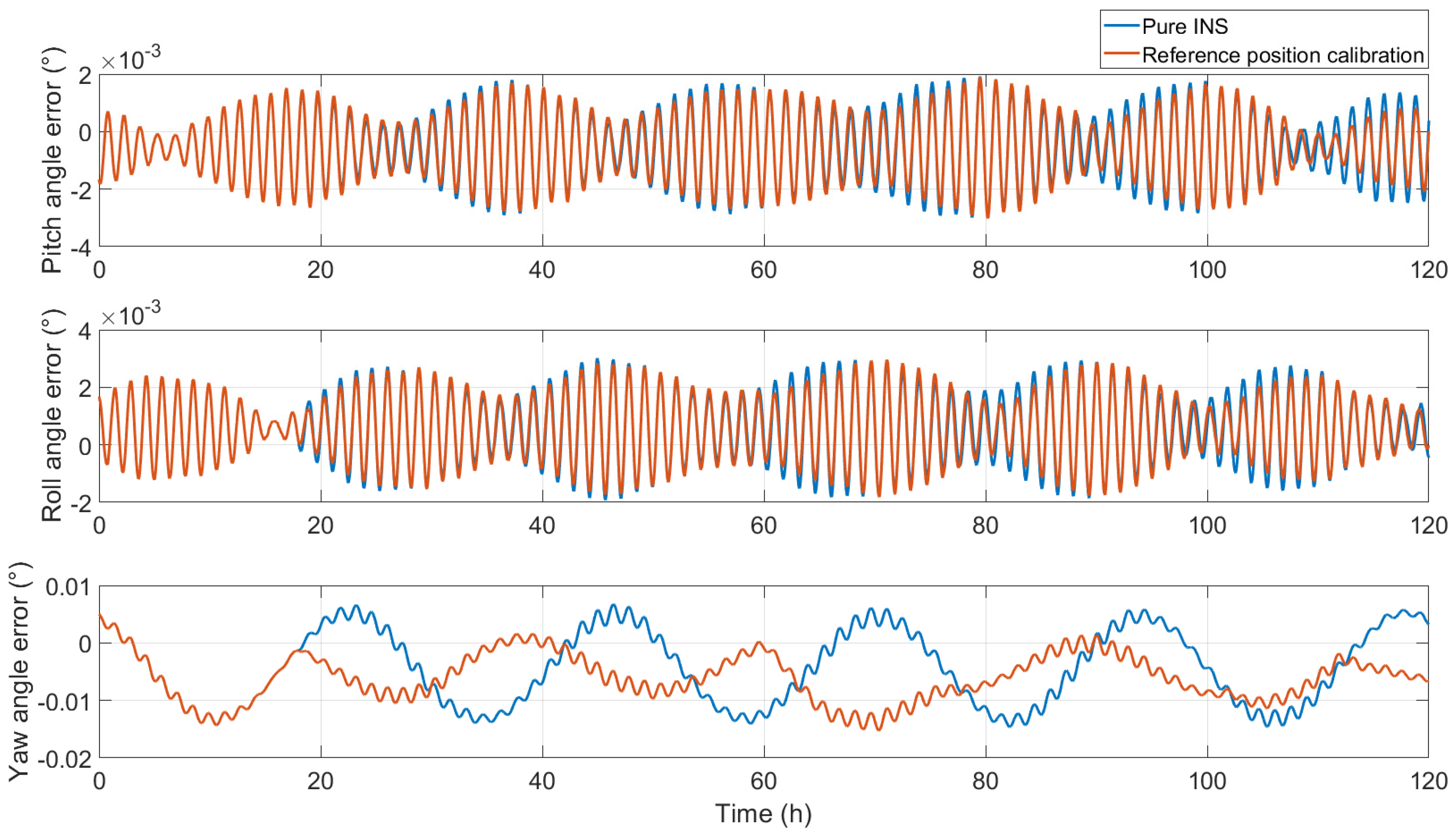
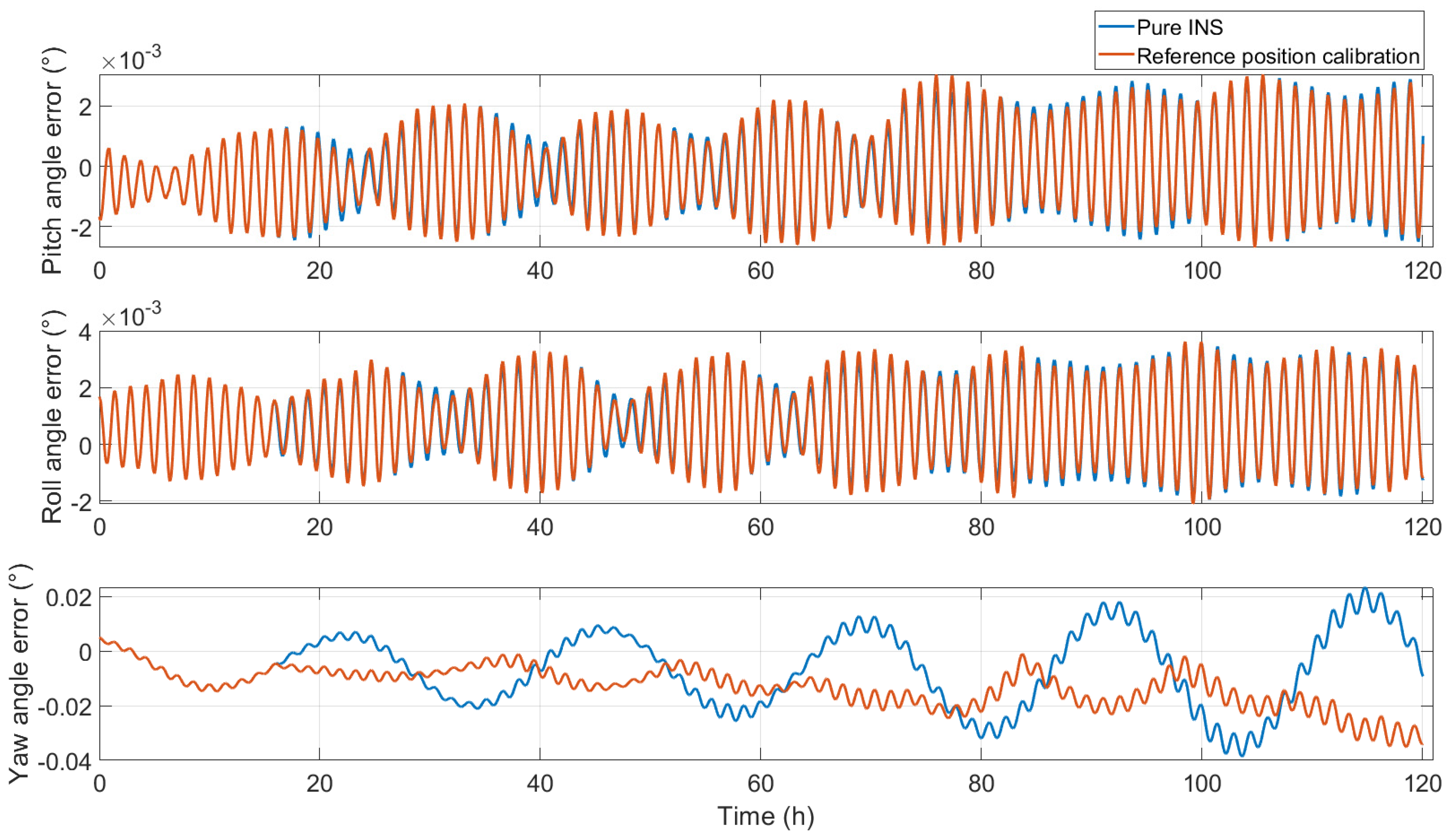
The attitude angle errors after reference position calibration are shown in Figure 1; from top to bottom, they are the pitch angle error, roll angle error, and azimuth angle error, respectively. The pitch angle and roll angle slightly change, whereas the yaw angle obviously changes because the yaw angle is directly affected after latitude calibration. This phenomenon can be explained by the principle of yaw damping [32]. The attitude angle error statistics are shown in

Table 3. Error statistics and accuracy evaluation of different methods under simulation static test conditions.

Navigation Error	Pure INS		Position Calibration		Accuracy Improvement
	Max	Std	Max	Std	Max	Std
Pitch angle error ($″$)	10.7594	4.2816	10.8561	4.0791	0.89% ↓	4.73% ↑
Roll angle error ($″$)	10.8463	4.3613	10.6492	4.1384	1.82% ↑	5.11% ↑
Yaw angle error ($″$)	52.6742	23.4260	54.9406	14.5905	4.13% ↓	37.72% ↑
East velocity error (m/s)	0.3961	0.1652	0.3711	0.1557	6.31% ↑	5.75% ↑
North velocity error (m/s)	0.3786	0.1663	0.3527	0.1552	6.84% ↑	6.67% ↑
Latitude error ($\mathrm{n} \mathrm{mile}$)	0.6644	0.3250	0.6644	0.2245	0% ↑	30.92% ↑
Longitude error ($\mathrm{n} \mathrm{mile}$)	8.2168	\	1.1629	\	85.85% ↑	\
Position error ($\mathrm{n} \mathrm{mile}$)	8.2168	\	1.2003	\	85.39% ↑	\

“↑“ represents an improvement in accuracy, while “↓“ represents a decrease in accuracy, and "\" indicates that no statistics should be conducted.

.

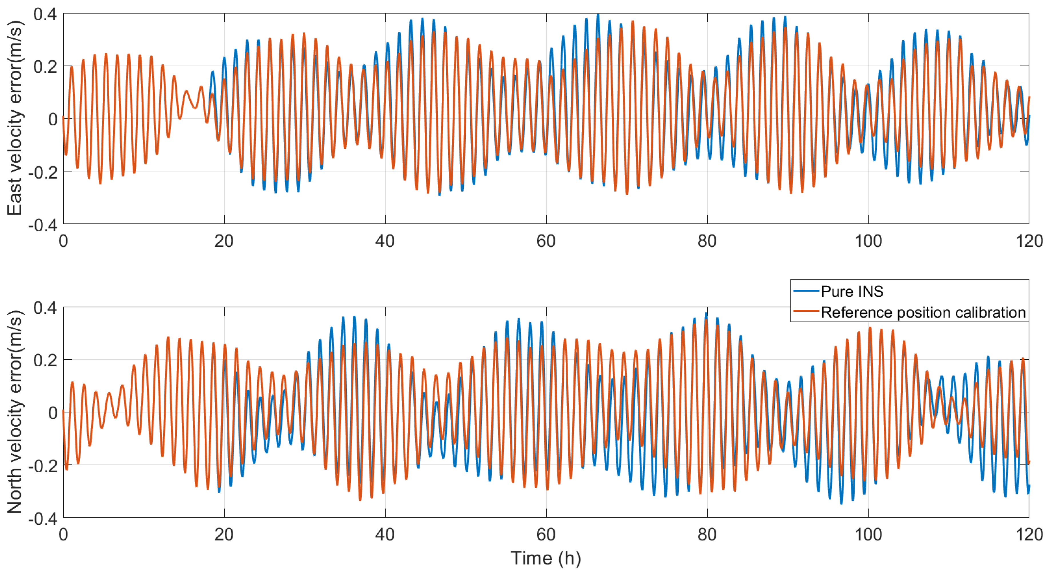
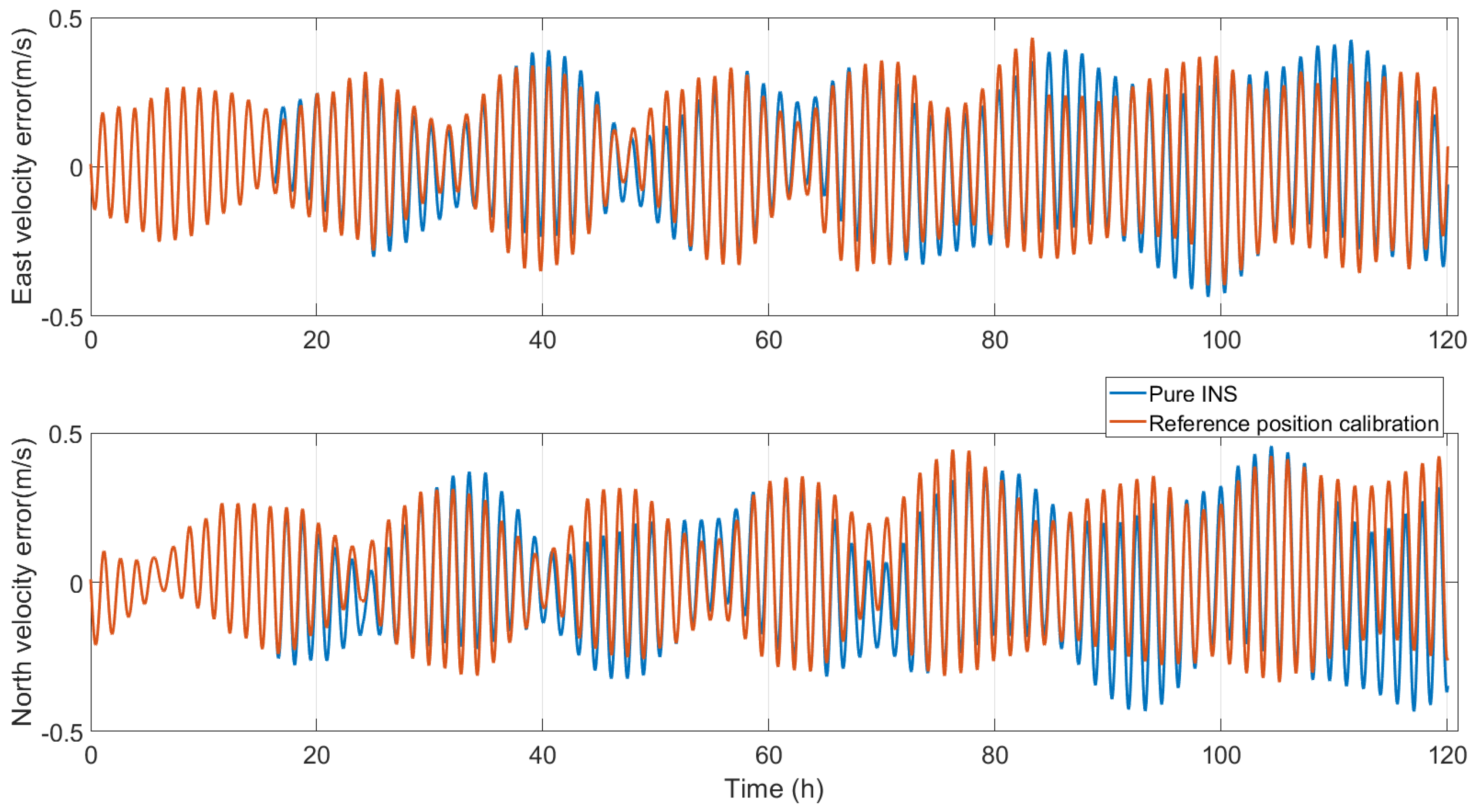
The variation in the velocity errors is shown in Figure 2. Overall, the velocity changes little after the reference position calibration; the main change is in the oscillation amplitude, and there is also a slight change in the phase. The velocity error statistics are shown in Table 3.

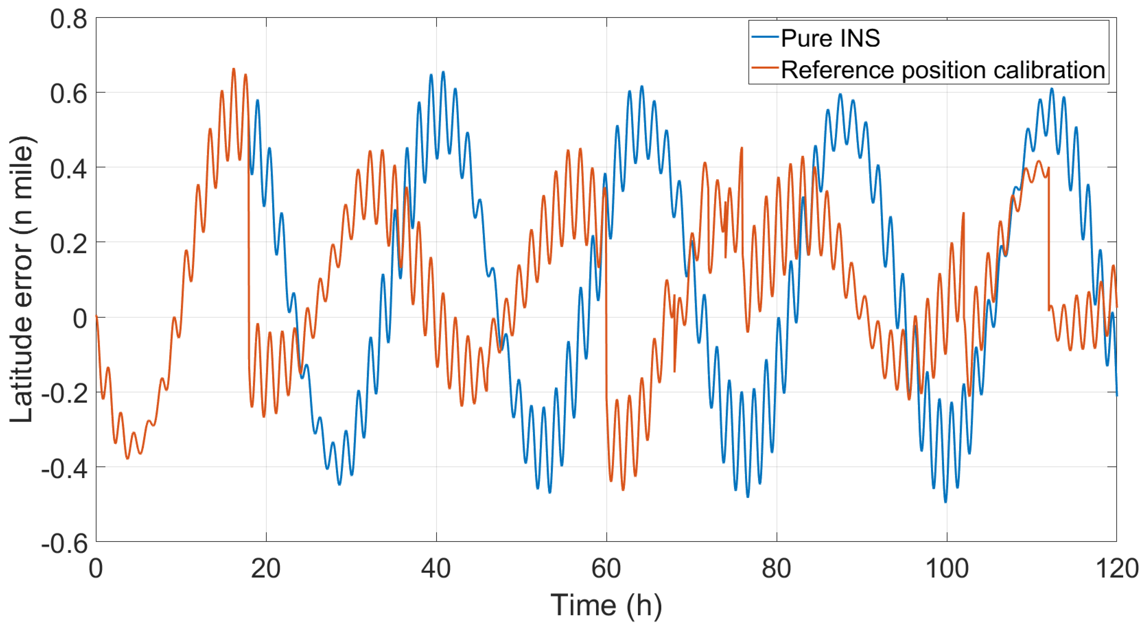
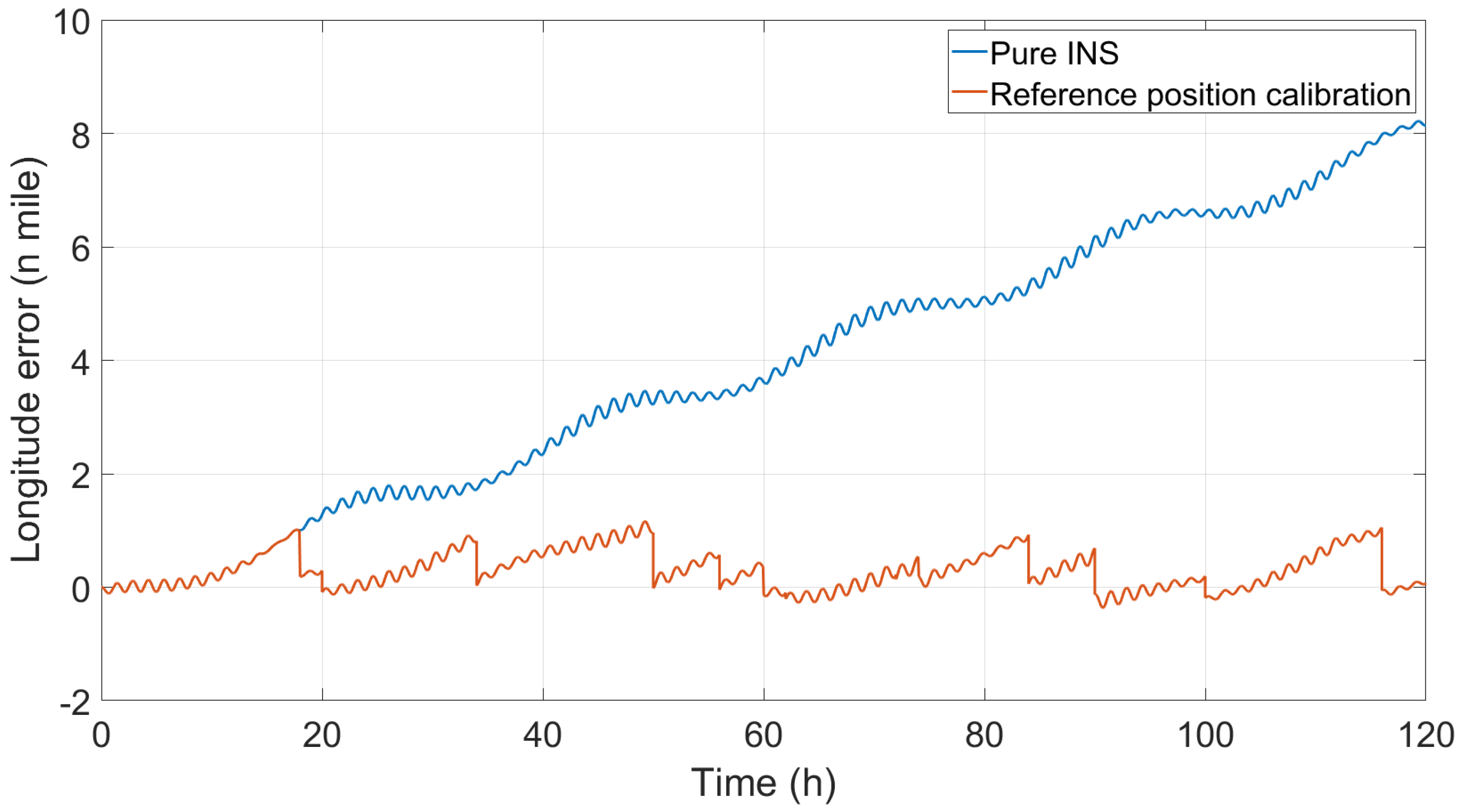
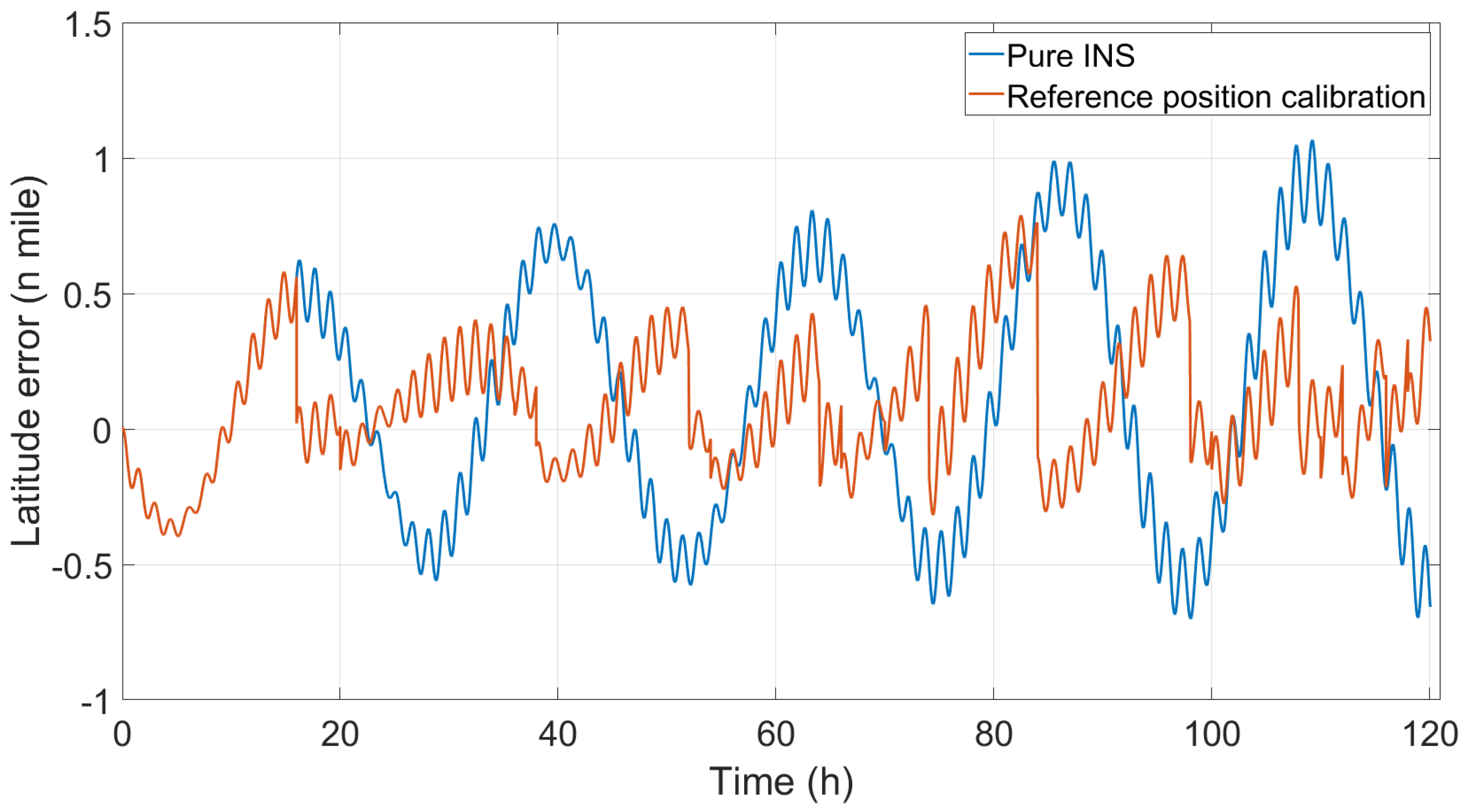
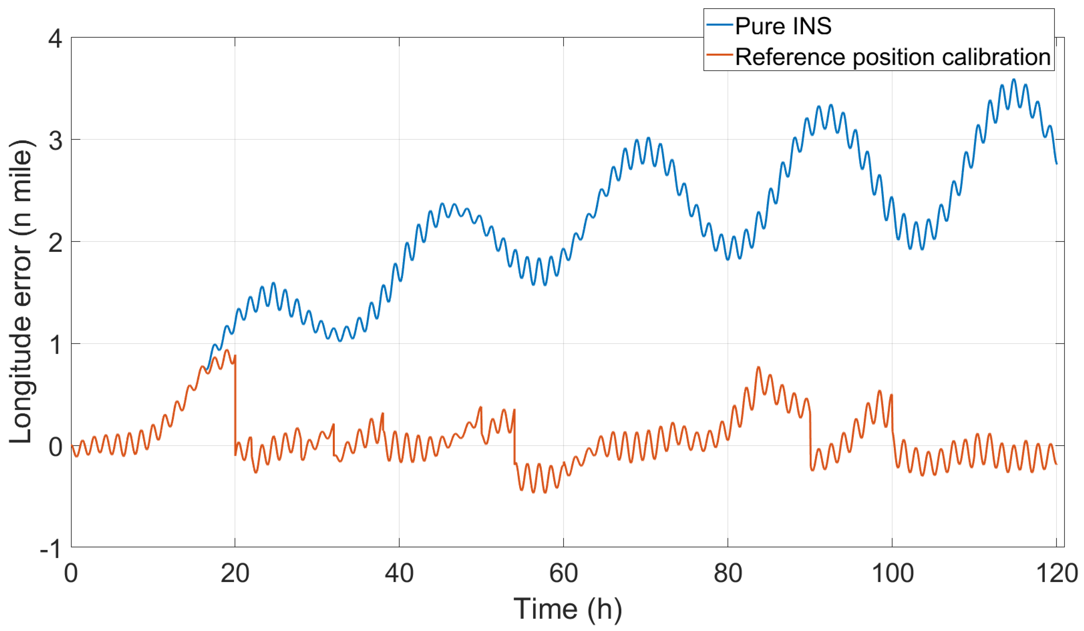
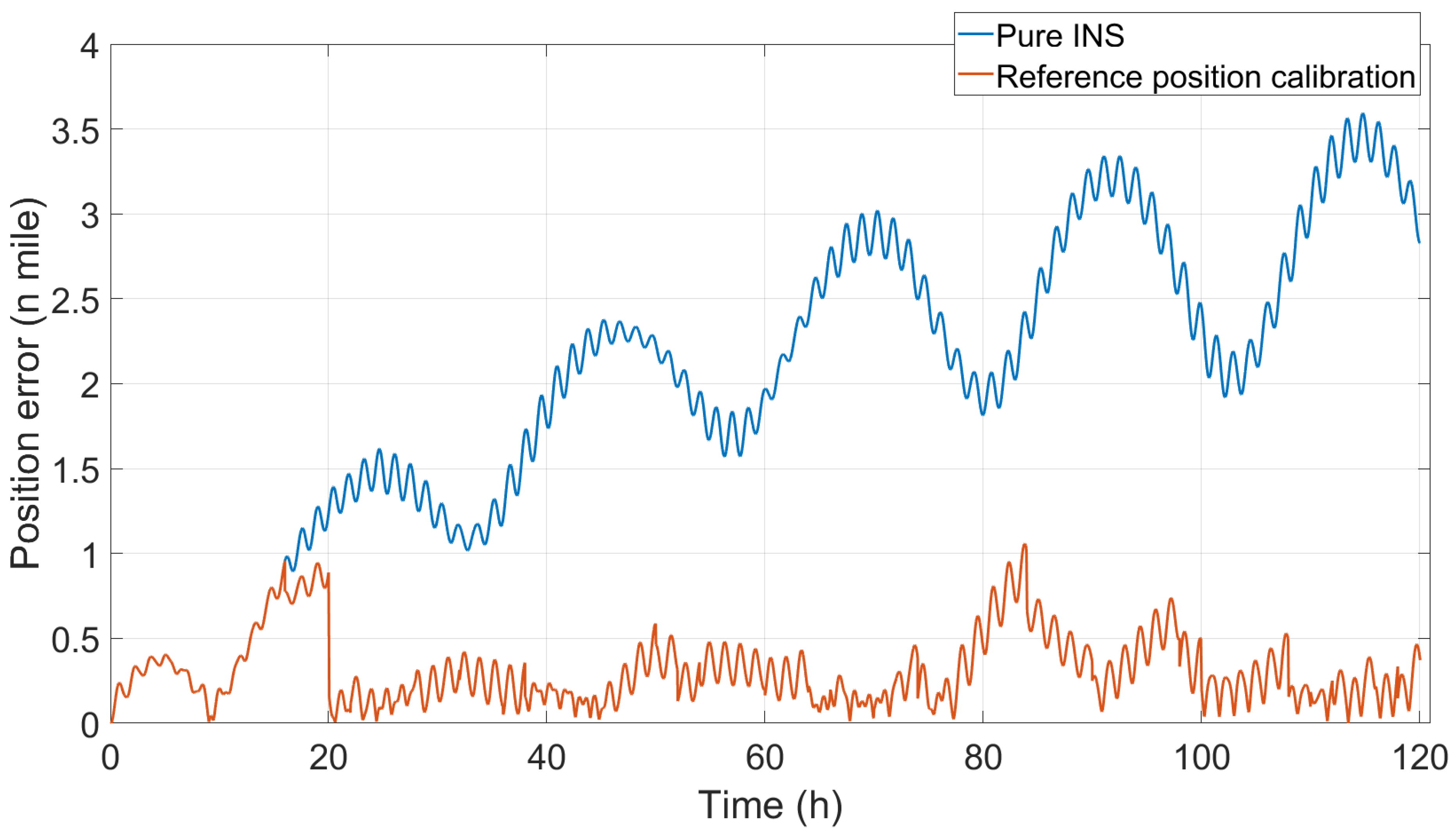
Figure 3, Figure 4 and Figure 5, respectively, show the latitude error, longitude error, and the position error that comprehensively considers the latitude error and longitude error. Because the INS position is calibrated directly, the INS position clearly changes, and the oscillation amplitude of the latitude error decreases, as shown in Figure 3; this indicates that the latitude calibration is correct. The trend of the longitude error increasing with time is suppressed, as shown in Figure 4; this indicates that the longitude calibration is correct. In the longitudinal direction, the greatest influence of the error is the trend item that grows over time, so the std value of the longitudinal error is not considered; rather, only the max value is calculated. As time goes by, the influence of the longitude error on the position error will become increasingly greater, and the position error will more prominently reflect the characteristics of the longitude error. As can be seen from Figure 5, the trend of the continuous growth of the position error over time has also been significantly suppressed. Similarly, only the max value of the position error is considered, and the statistical results are shown in Table 3.

First, the statistical results of the attitude angle errors are analyzed. After position calibration, the pitch angle error max value changed from 10.7594 $″$ to 10.8561 $″$, the value slightly increased, and the accuracy decreased by 0.89%. The std value changed from 4.2816 $″$ to 4.0791 $″$; the value decreased, and the accuracy improved by 4.73%. The roll angle error max value changed from 10.8463 $″$ to 10.6492 $″$, the value decreased, and the accuracy improved by 1.82%. The std value changed from 4.3613 $″$ to 4.1384 $″$; the value decreased, and the accuracy improved by 5.11%. The yaw angle error max value changed from 53.6742 $″$ to 54.9406 $″$; the value increased, and the accuracy decreased by 4.13%. The std value changed from 23.4260 $″$ to 14.5905 $″$; the value decreased, and the accuracy improved by 37.72%. The max values of the pitch angle and yaw angle are slightly larger than those of the pure INS, whereas the max values of the roll angle are slightly smaller. However, the standard deviation of the three attitude angles decreases, indicating that the fluctuation in the attitude angle error decreases after position calibration, especially the change in the yaw angle. This is consistent with the rule in Figure 1. The pitch angle and roll angle change slightly before and after position calibration, but the yaw angle clearly changes.

For the statistical results of the velocity error, after position calibration, the east velocity error max changed from 0.3961 m/s to 0.3711 m/s; the value decreased, and the accuracy improved by 6.31%. The std value changed from 0.1652 m/s to 0.1557 m/s; the value decreased, and the accuracy improved by 5.75%. The north velocity error max value changed from 0.3786 m/s to 0.3527 m/s; the value decreased, and the accuracy improved by 6.84%. The std value changed from 0.1663 m/s to 0.1552 m/s; the value decreased, and the accuracy improved by 6.67%. Both the max and std values decrease after position calibration. The decrease in the std value also indicates that the fluctuation in the velocity error decreases. The most important factor is the statistical result of the position error because the position is directly calibrated. Table 3 shows that the maximum latitude error does not change and that the std value decreases. The latitude error max value changed from 0.6644 $\mathrm{n} \mathrm{mile}$ to 0.6644 $\mathrm{n} \mathrm{mile}$; the value remained unchanged, and the accuracy was improved to 0%. The std value changed from 0.3250 $\mathrm{n} \mathrm{mile}$ to 0.2245 $\mathrm{n} \mathrm{mile}$; the value decreased, and the accuracy improved by 30.92%. Combined with Figure 3, this is because the maximum latitude error appeared before calibration in terms of the numerical value, and after position calibration, the maximum latitude error significantly decreased, and the fluctuation also decreased. The longitude error max value changed from 8.2168 $\mathrm{n} \mathrm{mile}$ to 1.1629 $\mathrm{n} \mathrm{mile}$; the value decreased, and the accuracy improved by 85.85%. The position error max value changed from 8.2168 $\mathrm{n} \mathrm{mile}$ to 1.2003 $\mathrm{n} \mathrm{mile}$; the value decreased, and the accuracy improved by 85.39%. Obviously, the longitude error and position error max value are significantly reduced.

4.2. Simulation Dynamic Test

In the simulation dynamic test, the inertial device error setting and initial error setting are the same as those in the simulation static test, as shown in Table 1 and Table 2, respectively. The simulation of the reference position is generated in the same way as the simulation static test. The carrier travel path is as follows: first, travel northward for 1 day, then move in the direction of 30° east of north for 2 days, and finally, follow a direction of 60° east of north for another 2 days. There is a short turning smoothing time in the above process. The test results are shown in Figure 6, Figure 7, Figure 8, Figure 9 and Figure 10.

Overall, the variation in the attitude angle errors are very similar to the simulation static test results, and the variation in the pitch angle error and roll angle error is very small, which indicates that direct INS position calibration has little influence on the pitch angle and roll angle, whereas the yaw angle error obviously changes, and the amplitude of the Earth periodic oscillation is suppressed, as shown in Figure 6. The specific statistical results are shown in

Table 4. Error statistics and accuracy evaluation of different methods under simulation dynamic test conditions.

Navigation Parameter Error	Pure INS		Position Calibration		Accuracy Improvement
	Max	Std	Max	Std	Max	Std
Pitch angle error ($″$)	10.6962	4.9015	10.9735	4.9755	2.53% ↓	1.49% ↓
Roll angle error ($″$)	12.9578	4.8825	13.0270	4.9900	0.53% ↓	2.15% ↓
Yaw angle error ($″$)	139.0604	47.6391	126.4014	26.1073	9.10% ↑	45.20% ↑
East velocity error (m/s)	0.4353	0.1864	0.4324	0.1855	0.67% ↑	0.48% ↑
North velocity error (m/s)	0.4561	0.1866	0.4441	0.1814	2.63% ↑	2.79% ↑
Latitude error ($\mathrm{n} \mathrm{mile}$)	1.0664	0.4501	0.7883	0.2384	26.08% ↑	47.03% ↑
Longitude error ($\mathrm{n} \mathrm{mile}$)	3.5907	\	0.9383	\	73.87% ↑	\
Position error ($\mathrm{n} \mathrm{mile}$)	3.5931	\	1.0581	\	70.55% ↑	\

“↑“ represents an improvement in accuracy, while “↓“ represents a decrease in accuracy, and "\" indicates that no statistics should be conducted.

.

The velocity error variation after reference position calibration are shown in Figure 7, which is close to the result of the pure INS, indicating that position calibration has little influence on velocity.

After position calibration, the Earth oscillation in terms of latitude is suppressed to a certain extent, as shown in Figure 8, which is very similar to the result of the yaw error. The trend item of the longitude error increasing with time has also been significantly suppressed, as shown in Figure 9. The situation of the position error is similar to that of the longitude error, as shown in Figure 10, which can greatly improve the navigation and positioning ability of INSs for long endurance. The detailed statistical results are shown in Table 4.

For the attitude angle error, after position calibration, the pitch angle error max value changed from 10. 6962 $″$ to 10.9735 $″$; the value slightly increased, and the accuracy decreased by 2.53%; the std value changed from 4.9015 $″$ to 4.9755 $″$; the value increased, and the accuracy decreased by 1.49%. The roll angle error max value changed from 12.9578 $″$ to 13.0270 $″$; the value increased, and the accuracy decreased by 0.53%; the std value changed from 4.8825 $″$ to 4.9900 $″$; the value decreased, and the accuracy decreased by 2.15%. The yaw angle error max value changed from 139.0604 $″$ to 126.4014 $″$; the value decreased, the accuracy improved by 4.13%; the std value changed from 47.6391 $″$ to 26.1073 $″$; the value decreased, and the accuracy improved by 45.20%. Compared with the results of the pure INS, the max and std values of the pitch angle and roll angle are both larger after reference position calibration, but the magnitude is very small, which is consistent with the results reflected in Figure 6, and the max and std values of the yaw angle are significantly reduced, which is also consistent with the results in Figure 6.

The east velocity error max value changed from 0.4353 m/s to 0.4324 m/s; the value decreased, and the accuracy improved by 0.67%. The std value changed from 0.1864 m/s to 0.1855 m/s; the value decreased, and the accuracy improved by 0.48%. The north velocity error max value changed from 0.4561 m/s to 0.4441 m/s; the value decreased, and the accuracy improved by 2.63%. The std value changed from 0.1866 m/s to 0.1814 m/s; the value decreased, and the accuracy improved by 2.79%. The max and std values of both the east velocity and the north velocity decrease after reference position calibration.

The latitude error max value changed from 1.0664 $\mathrm{n} \mathrm{mile}$ to 0.7883 $\mathrm{n} \mathrm{mile}$; the value remained unchanged, and the accuracy was improved to 26.08%. The std value changed from 0.4501 $\mathrm{n} \mathrm{mile}$ to 0.2384 $\mathrm{n} \mathrm{mile}$; the value decreased, and the accuracy improved by 47.03%. The longitude error max value changed from 3.5907 $\mathrm{n} \mathrm{mile}$ to 0.9383 $\mathrm{n} \mathrm{mile}$; the value decreased, and the accuracy improved by 73.87%. The position error max value changed from 3.5931 $\mathrm{n} \mathrm{mile}$ to 1.0581 $\mathrm{n} \mathrm{mile}$; the value decreased, and the accuracy improved by 70.55%. The max and std values of the latitude error are also significantly smaller, and the max value of the longitude error and position error are also significantly reduced, which indicates that the position calibration method proposed in this paper is effective and significantly improves the navigation and positioning ability of the INS for long-term endurance.

5. Conclusions

Because continuous, stable, and high-precision position information is not easy to obtain in practical applications, this paper proposed a position calibration method for INSs that is based on sparse and low-precision position information. On the basis of the analysis of the INS error law, a judgment method was given to determine whether sparse and low-precision position information is available. The effectiveness of the proposed method was verified via static and dynamic simulation tests. Intuitively, the effect of this method on the attitude angle is not obvious. This is because the attitude angles were not directly calibrated. Although the statistical results of the max and std values show that after position calibration, some of them are even larger, the magnitude is very small, and the effect of this method on velocity is not obvious. Similarly, this is because there is no direct calibration of the velocity; however, the max and std values are reduced, and the position error is more obvious. In the simulation static test, the max value of the longitude error decreased from 8.2168 $\mathrm{n} \mathrm{mile}$ to 1.1629 $\mathrm{n} \mathrm{mile}$, and the accuracy improved by 85.85%; the max value of the position error decreased from 8.2168 $\mathrm{n} \mathrm{mile}$ to 1.2003 $\mathrm{n} \mathrm{mile}$, and the accuracy improved by 85.39%. In the simulation dynamic test, the max value of the longitude error decreased from 3.5907 $\mathrm{n} \mathrm{mile}$ to 0.9383 $\mathrm{n} \mathrm{mile}$, and the accuracy improved by 73.87%; the max value of the position error decreased from 3.5931 $\mathrm{n} \mathrm{mile}$ to 1.0581 $\mathrm{n} \mathrm{mile}$, and the accuracy improved by 70.55%.

The max values of longitude and position errors were suppressed. The simulation static test and dynamic test demonstrated that the comprehensive calibration method proposed in this paper can suppress the cumulative errors in INSs based on sparse and low-precision position information. This method can effectively improve the autonomous navigation and positioning ability of underwater vehicles during long-term endurance navigation.

It can be seen from the simulation results that the method proposed in the paper realizes the effective utilization of sparse and low-precision position information, and ensures the consistency of the calibration effect as a whole. Although from the statistical results of the attitude angles, some indicators have become larger, in fact, the values are very small, which is acceptable.

The test results are in line with expectations. Since the external auxiliary position is judged and then the INS position is directly calibrated, the suppression effect of the position error will be the most obvious after comprehensive calibration. This is also one of the most concerned parameters for the safe navigation of underwater submersibles. The advantage of this method lies in its simplicity and feasibility. It effectively utilizes sparse and low-precision position information, avoids the damage of outliers to INSs, and has important application value.

6. Discussion

Overall, the means of navigation and positioning in marine navigation scenarios are much fewer than those in land navigation scenarios, especially in underwater navigation. Due to the influence of the complex marine environment, underwater navigation and positioning still face significant challenges. Since INSs can hardly be used as a single sensor in long-voyage navigation tasks but require external auxiliary information for calibration, it is natural to consider the characteristics of the auxiliary information, such as continuity and accuracy. There are relatively mature solutions for INS calibration using continuous and high-precision auxiliary information. The method proposed in this paper is mainly used to solve the problem of INS calibration using sparse and low-precision position information, which has important practical significance and engineering application value.

An important application scenario of the method proposed in this paper is marine navigation, especially underwater navigation. This has been described in detail in Section 1, particularly with respect to the GAINS. The GAINS is a mainstream autonomous passive positioning method, and it has significant application value in the military field. Currently, the precision of gravity matching results is basically at the level of hundreds of meters or even larger. Many factors affect the accuracy of gravity matching, such as the accuracy and resolution of the gravity database, the gravity change characteristics of the matching area, the real-time measurement accuracy of gravity, and the gravity matching algorithm. However, the ultimate goal of the GAINS is to calibrate the INS after a matching position is obtained. Therefore, which matching positions can be used for calibration and how to perform the calibration are also important aspects. This is one of the main issues that this paper focused on and aimed to address. The matching positions from the GAINS conform to the characteristics of sparsity and low precision. In fact, the matching position is the reference position in the simulation test. In practical applications, the matching position needs to be combined with the INS position for comprehensive judgment, and then the matching position that meets the conditions is selected for INS calibration.

Although this is illustrated with the GAINS as an example, it should be noted that this method is universal and can also be extended to other application scenarios. Under special environments, only sparse and low-precision position information can be obtained, and as long as the external auxiliary information conforms to the comprehensive judgment method proposed in this paper, it can be used for INS calibration.

There are two shortcomings of this method. The first one is that the judgment conditions might be overly strict. Strict judgment conditions are aimed at obtaining available reference positions, avoiding damage to INSs, and thus ensuring the safety of navigation. However, at the same time, this will also reduce the utilization rate of reference information. Therefore, improving the judgment conditions is a direction for future research. The second is that the suppression effect of this method on the attitude angle and velocity errors is not obvious. Therefore, conducting comprehensive processing in combination with other data is another direction for future research.

In marine navigation applications, the Doppler velocity log (DVL) is also a common auxiliary item of equipment that can provide velocity information and has two working modes: one is to provide the velocity of the seabed, which is highly accurate but difficult to achieve in deep sea areas; the other is to provide the velocity of the current. This mode is affected by the marine environment, and the accuracy is limited [33,34,35]. The next research focus is how to use the DVL effectively to further improve the INS positioning accuracy on the basis of this paper.