Using the Debiased Brier Skill Score to Evaluate S2S Tropical Cyclone Forecasting

Abstract

To evaluate tropical cyclone forecasting on synoptic timescale, tracking and intensity are used. On subseasonal to seasonal (S2S) timescale, what aspects of tropical cyclones should be predicted and how to evaluate forecasting skills still remain open questions. Following our previous work, which proposed using daily tropical cyclone probability (DTCP) as a measure of tropical cyclone activity and the debiased Brier skill score (DBSS) to evaluate tropical cyclone forecasting on S2S timescale, the present research investigates the influence of several factors that may influence the use of DTCP and the DBSS framework. These factors are the forecast time window, tropical cyclone influence radius, evaluation region, forecast sample, and how the Brier score for the reference climate forecast is computed. The influence of these factors is discussed based on the output of the S2S prediction project database and comparison of the DBSS when the above factors are changed individually. Changes in the forecast time window, evaluation region, and tropical cyclone influence radius can change the DTCP. The larger the tropical cyclone influence radius and the longer the forecast time window, the larger the DTCP will be. However, the spatially averaged DBSS changes very little. Using estimated Brier score for reference climate forecast can cause variation due to limited forecast samples. It is recommended to use the theoretical value of the Brier score for reference climate forecasting, instead of its estimation.

1. Introduction

The annual tropical cyclone (TC)-related coastal risk and associated destructive losses continue to rise [1,2,3,4]. Due to improvements in numerical modeling, forecasting skills for extreme events have been substantially enhanced [5], contributing to better TC monitoring.

Subseasonal-to-seasonal (S2S) prediction is generally defined as including forecasts spanning beyond 14 days but less than a season (14 days to 3 months). Previously, S2S forecasting was often referred to as a “predictability desert”, representing a significant gap between weather and climate prediction [6]. This gap arises because the S2S scale is too long for the atmosphere to retain sufficient memory of initial conditions, unlike the synoptic scale. Conversely, relative to seasonal scale, the S2S scale is too short to fully capture the coupling signals of boundary condition anomalies. This disparity is further reflected in the lack of operational forecasting products bridging the gap between weather and seasonal prediction.

However, recent technological advancements and growing demand for S2S predictions have renewed people’s interest in this field [7]. An increasing number of research institutions are now focusing on S2S forecasting, and improvements in numerical models have uncovered new sources of predictability, significantly enhancing forecasting skills. Under the leadership of the World Meteorological Organization (WMO), multiple countries and research institutions have collaborated on S2S prediction across various domains, particularly for extreme events, such as in TC forecasting. Nevertheless, challenges remain, including inconsistencies in the TC variables used across different institutions.

S2S TC forecasting plays a crucial role between synoptic forecasting and seasonal forecasting. However, the transition of S2S TC forecasting from research to operational applications has been slow, partly due to the absence of standardized operational practice [8]. To advance research, improve forecasting skills, and expand the scope of operational S2S forecast, the World Weather Research Programme (WWRP) and the World Climate Research Programme (WCRP) under the WMO jointly launched a ten-year (2013–2023) initiative known as the S2S Prediction Project [9,10]. The project aimed to bridge the gap between medium-range weather forecasting and seasonal prediction while improving the understanding of S2S predictability sources. Phase I of the S2S Prediction Project (2013–2017) focused on establishing the S2S database, which included hindcast data from 11 centers [11]. The project was subsequently extended into Phase II (2018–2023). A key component of Phase II was real-time prediction (RTP), which aimed to provide real-time S2S forecasts for broader geographical regions and applications [12]. Though the Phase II project was officially concluded at the end of 2023, many institutions still continue to provide their S2S forecast products.

Various TC variables and evaluation metrics have been used to evaluate S2S TC forecasting. In one early research project, the hindcast from the European Centre for Medium-Range Weather Forecasts (ECMWF) was used to assess weekly TC occurrences in different regions of the Southern Hemisphere, employing the Brier skill score (BSS) as the evaluation metric [13]. Subsequent work [14] introduced a series of TC forecast products from ECMWF, including “strike” probability and TC probability maps. The “strike” area was defined as within 120 km of the TC track. Additionally, probability maps for TC activity (including genesis) were provided for wind speeds exceeding 17 m/s and 33 m/s, calculated over a 7-day time window, with a TC influence radius of 300 km. A TC track verification method was developed using ECMWF forecasts in the North Atlantic (ATL), matching them with best-track datasets [15]. Although the model captured nearly all TCs during two TC seasons, substantial errors persisted, which underscores the inapplicability of using TC track for S2S prediction.

Probabilistic forecasts for TC activity (genesis and movement) using a 3-day sliding window and a 300 km TC influence radius were validated with BSS within 14 days [16]. The results demonstrated that models could provide skillful TC predictions beyond the second week, outperforming climatological forecasts. Monthly TC forecasts from the Geophysical Fluid Dynamics Laboratory High-Resolution Atmospheric Model were evaluated in ATL by TC frequency and Accumulated Cyclone Energy (ACE) [17]. However, the monthly resolution limited precise description of TC location.

Recent studies evaluating S2S TC forecasts have described TC activity within a “Box” (20° longitude × 15° latitude). Both the probability of TC occurrence and the frequency of genesis have been utilized to assess multi-model hindcasts from the S2S database on a weekly basis [18]. Evaluations employed the ACE and BSS, using two different reference forecasts including monthly varying climatology. The Australian Bureau of Meteorology’s seasonal forecasting systems (ACCESS-S2) were applied to predict weekly global TC activity [19]; the results showed that BSS varied across different time periods, and different calibration methods failed to improve the ACCESS skill. This indicates that differences in forecast samples lead to irreducible systematic variations that affect skill scores. Similarly, multi-week TC forecasts during the 2017–2019 Southern Hemisphere TC seasons were also evaluated using real-time predictions from ACCESS-S [20,21]. It was found that models with larger ensemble sizes, higher spatial resolution, and better initialization schemes exhibited better forecasting skill.

Daily tropical cyclone probability (DTCP) was proposed as a forecast variable and used to systematically evaluate 11 models in the S2S reforecast database for the Western North Pacific (WNP) via debiased Brier skill score (DBSS) and Taylor score [22]. The evaluation of S2S TC activity forecasts using NOAA’s Global Ensemble Forecast System and ECMWF hindcasts for the ATL emphasized the impact of ensemble size on the model’s skill. [23]. Genesis Potential Index (GPI) and DBSS were applied to assess NASA’s GEOS-S2S-2 hindcasts for the ATL over a 30-day lead time [24]. The growing interest in S2S prediction led to the SubX subseasonal experiment [25], designed to integrate multi-model ensembles for S2S forecasting, mainly for the ATL region. SubX combines hindcast data from seven global models, leveraging their strengths to enhance prediction accuracy.

A recent review [26] summarized progress in S2S TC forecasting and highlighted multi-model TC forecast data from various databases. However, methods for evaluating TC forecasts remain diverse. As mentioned earlier, most S2S TC forecast products are probabilistic, but the application of probabilistic methods and the impact of different evaluation criteria on results require further exploration. Therefore, this study examines TC forecast data from four models in the S2S real-time database, testing and evaluating multiple factors influencing the models’ forecasting skills. Clarifying the influence of these factors will enhance the societal application of TC forecasting. The WNP is the most active basin for TC globally [27]. On average, approximately 30 TCs occur annually in the WNP, accounting for over 30% of the global annual total of about 80 TCs [28] and contributing to roughly 40% of the worldwide ACE [29]. TC activity in the WNP exhibits remarkable complexity. Given these characteristics, this study used forecast products from the WNP to conduct tests with these factors changed individually, one by one. This paper is organized as follows. Materials and methods for the S2S TC forecasting skills evaluation test are described in Section 2, and the results of different test cases are reported in Section 3, followed by conclusions in Section 4.

2. Materials and Methods

2.1. Observational Tropical Cyclone Data

The International Best Track Archive for Climate Stewardship (IBTrACS) is an integrated dataset of historical TC activities [30]. The dataset combines all available information from buoys, offshore observation platforms, satellites, etc. IBTrACS unifies data from different institutions and different ocean basins, providing a global TC track database. The latest version of the dataset is 4.0, which includes a time interval of 3 h for all TC tracks. This study used data on the position of TC centers, maximum sustained wind speeds, and minimum pressure at cyclone centers. We calculated the observed DTCP from the TC center position information (longitude and latitude).

2.2. S2S Real-Time Database

Table 1. Details of 4 models that provided forecasts in the WMO S2S real-time prediction project. These models started to provide their forecasts in different years (Column 4) and include different forecasting samples (Column 2). The frequency of forecasts (Column 6) and numbers of ensemble members (Column 5) are also shown.

System	Forecast Samples	Lead Time (Day)	Period (Year)	Ensemble Size	Frequency
ECMWF	473	46	2015–2023	51	Twice/week
KMA	1656	60	2015–2023	4	Daily
NCEP	1656	44	2015–2023	16	Daily
UKMO	1452	60	2016–2023	4	Daily

provides the relevant information regarding the real-time forecast models. The 4 models selected were those from the European Centre for Medium-Range Weather Forecasts (ECMWF), the Korea Meteorological Administration (KMA), the United States National Centers for Environmental Prediction (NCEP), and the United Kingdom Met Office (UKMO). These models started providing their real-time products in different years (Column 4), and they also have different ensemble members (Column 5). Moreover, the models have different forecast frequencies (Column 6) and numbers of forecast samples (Column 2). All these details could influence evaluation of the forecasting skill of specific models [26,31]. The forecast lead time also varies (Column 3). Thus, our evaluation test calculation was for forecasts with lead time up to 30 days.

Based on previous research [16,18,22], the ECMWF model is generally considered to have better forecasting skills; so, its real-time TC forecasting data are representative for conducting experiments. When testing the impact of forecast frequency, we additionally selected three daily forecast models to make the experiment robust. The same TC tracker was applied to all these S2S models [32]. The models’ DTCP was computed based on the results of the TC tracker for each ensemble member and these values were used in our test. Because most TCs happen in summer or autumn, we used only the forecasting samples from May to October for the WNP. Though there are around a dozen institutions that provide their forecasts in real time, only these four were selected for the present research. The reason for this is that the ECMWF model tends to have high S2S TC forecasting accuracy and the models from KMA, NCEP and UKMO produce forecasts daily, providing a larger forecast sample than the other models from the S2S database that have lower frequency (weekly or bi-weekly).

2.3. Daily Tropical Cyclone Probability

When evaluating TC forecasting on the S2S timescale, several factors may influence the evaluation. This study utilized the DTCP proposed previously [22] to find out how these factors affected forecasting skill. DTCP is defined as the probability of TC occurrence within a specific TC influence radius of a location and 1 day forecast time window. We computed DTCP on a $1°\times 1°$ grid and tested the influence of factors such as TC influence radius, forecast time window, etc. The computation of DTCP from observation was based on the IBTrACS data being collected every three hours. When calculating the DTCP from the models, TC center positions predicted by each ensemble member were used to compute the DTCP for that ensemble member, and the final DTCP for the ensemble prediction system was the average of the DTCP fields of all ensemble members in the model. As an example, Figure 1 shows the DTCP predictions of Typhoons Noul and Dolphin made by the KMA model from 2 May to 7 May 2015. Due to the fact that the KMA ensemble forecasting system has 4 ensemble members, there are 5 possible outcomes for calculating DTCP based on the model (DTCP values of 0, 0.25, 0.5, 0.75, and 1).

2.4. Debiased Brier Skill Score

According to the definition of DTCP, the occurrence of a TC can be treated as a dichotomous event similar to precipitation, so it is possible to use the Brier skill score [33] to evaluate forecasting skills. A correction term is added to obtain the debiased Brier skill score, which corrects the negative bias caused by small ensemble members and makes it more suitable for ensemble forecasting systems [34]. The DBSS is defined as follows:

$$\mathrm{D}\mathrm{B}\mathrm{S}\mathrm{S}=1-{\displaystyle \frac{<\mathrm{B}\mathrm{S}>}{<{\mathrm{B}\mathrm{S}}_{\mathrm{C}\mathrm{L}}>+\mathrm{D}}}$$

(1)

where <BS> is the Brier score, which is the mean squared error calculated from forecast and observation; <∙> is the average over the forecast samples. The $<\mathrm{B}\mathrm{S}>$ can be computed directly as follows:

$$<\mathrm{B}\mathrm{S}>=\sum _{\mathrm{k}=1}^2\sum _{\mathrm{j}=1}^{\mathrm{N}}{\displaystyle \frac{{({\mathrm{Y}}_{\mathrm{k}\mathrm{j}}-{\mathrm{O}}_{\mathrm{k}\mathrm{j}})}^2}{\mathrm{N}}},$$

(2)

where k = 1, 2 is the number of categories (with and without TC in observation); ${\mathrm{Y}}_{\mathrm{k}\mathrm{j}}$ is the prediction for category k and sample j; ${\mathrm{O}}_{\mathrm{k}\mathrm{j}}$ is the observed DTCP for category k and sample j. The value of $<\mathrm{B}\mathrm{S}>$ changes from 0 to 2, with 0 as the perfect prediction and 2 as the situation when the prediction is wrong every time.

$<{\mathrm{B}\mathrm{S}}_{\mathrm{C}\mathrm{L}}>$ is the Brier score when a reference climate forecast is used; $<{\mathrm{B}\mathrm{S}}_{\mathrm{C}\mathrm{L}}>$ can be calculated theoretically via the following formula:

$$<{\mathrm{B}\mathrm{S}}_{\mathrm{C}\mathrm{L}\_\mathrm{t}\mathrm{h}\mathrm{e}\mathrm{o}\mathrm{r}\mathrm{y}}>=2\mathrm{p}·\left(1-\mathrm{p}\right).$$

(3)

On the other hand, $<{\mathrm{B}\mathrm{S}}_{\mathrm{C}\mathrm{L}}>$ can also be directly estimated based on forecast samples, according to the following formula:

$$<{\mathrm{B}\mathrm{S}}_{{\mathrm{C}\mathrm{L}}_{\mathrm{e}\mathrm{s}\mathrm{t}\mathrm{i}\mathrm{m}\mathrm{a}\mathrm{t}\mathrm{e}}}>=\sum _{\mathrm{k}=1}^2\sum _{\mathrm{j}=1}^{\mathrm{N}}{\displaystyle \frac{{\left({\mathrm{C}}_{\mathrm{p}}-{\mathrm{O}}_{\mathrm{k}\mathrm{j}}\right)}^2}{\mathrm{N}}}.$$

(4)

where ${\mathrm{C}}_{\mathrm{p}}$ is the climatological TC occurrence probability, either $\mathrm{p}$ or $1-\mathrm{p}$.

In Formula (3), $<{\mathrm{B}\mathrm{S}}_{\mathrm{C}\mathrm{L}\_\mathrm{t}\mathrm{h}\mathrm{e}\mathrm{o}\mathrm{r}\mathrm{y}}>$ is computed from $\mathrm{p}$, which is the climatological DTCP calculated from observation for the years when the model provided a forecast. It should be noted that in Formula (2), there is a summation over TC categories k, with and without TC activity, but in another formulation [23], there is no summation over TC category k. There is a difference in $<\mathrm{B}\mathrm{S}>$ and $<{\mathrm{B}\mathrm{S}}_{\mathrm{C}\mathrm{L}}>$ by a factor of 2 with and without summation over the category k. It should be noted that using summation over the category k is consistent with the derivation of the correction term D for ranked probability skill score [34].

In Formula (1), D is given as follows:

$$\mathrm{D}={\displaystyle \frac{\mathrm{p}·\left(1-\mathrm{p}\right)}{\mathrm{M}}}$$

(5)

where M is the number of ensemble members. D can correct negative bias that occurs when M is small, and its effect decreases when M becomes large [34].

The meaning of the DBSS is to compare the Brier score from model forecast with the Brier score of reference climate forecast if D is ignored for convenience. When the forecast from a model is better than the reference climate forecast, the DBSS is greater than 0. The model forecast can provide further valuable information compared with a straightforward reference climate forecast. We removed the grid points with $p$ below a certain threshold when computing the basin-averaged DBSS. Some grid points were removed before computing the basin-averaged DBSS to avoid exceptionally negative values at these points. Both the two terms in the denominator of Equation (1) have climatological DTCP $\mathrm{p}$. If $\mathrm{p}$ is zero, the value of DBSS at that point is not defined. If p is small, an exceptionally large negative DBSS may be generated.

3. Results

Probabilistic forecasting variables have been widely applied for evaluation of S2S TC prediction [14,16,18,22]. However, multiple factors in the computation can influence the evaluation results, such as the TC influence radius and forecast time window in DTCP. The lack of standardized calculation methods for these probabilistic forecasts poses significant challenges for the operational application of S2S TC prediction.

Previous studies have commonly employed the Brier skill score (BSS) and debiased Brier skill score (DBSS) to assess probabilistic forecasting skill. Nevertheless, the computational approaches of the terms in the above equation are different. This section systematically focuses on DTCP and DBSS to examine the factors affecting evaluation of the models’ forecasting skill, including different evaluation regions, varying forecast time windows, different TC influence radii, alternative methods for computing the Brier score of reference climate forecasts, and the application of the correction term D. Through comprehensive experiments, we analyzed the influence of these factors on DTCP and DBSS. In the initial framework [22], we used a definition of DTCP with a 1-day forecast time window and 500 km TC influence radius. Based on the four models’ forecast outputs (mainly the ECMWF model) in Table 1, we investigated the effect of removing the grid points where climatological $\mathrm{p}$ was below certain criteria, such as 0.01, and when a different forecast time window and TC influence radius were used. The influence of different methods to compute $<{\mathrm{B}\mathrm{S}}_{\mathrm{C}\mathrm{L}}>$ and whether to include correction term D are also analyzed.

3.1. Test of Evaluation Region for Basin Averaged DBSS

A mask was implemented in the calculation of basin-averaged DBSS to exclude grid points with observed climatological DTCP $p$ below specified thresholds. This prevented the potential influence of exceptionally large negative DBSS values due to extremely low $p$ values at certain grid points.

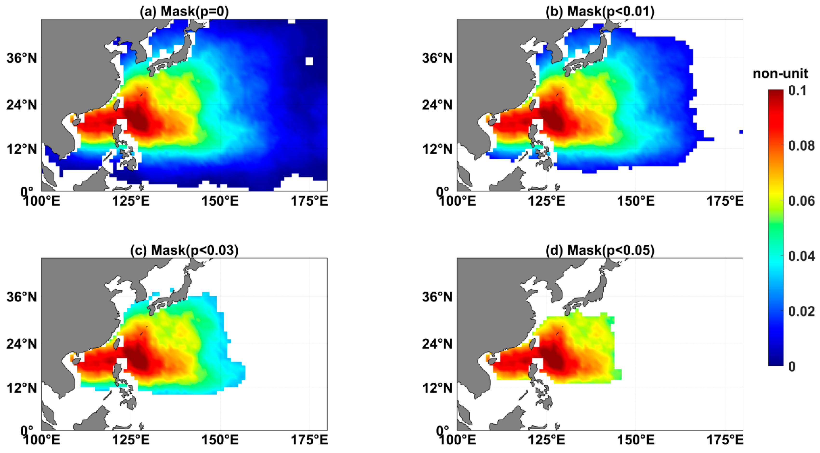
The selection of different thresholds inherently defines varying evaluation regions; higher thresholds correspond to oceanic regions with more TC activity. To systematically evaluate the sensitivity of DBSS to different evaluation regions, we examined four threshold values: 0 (Figure 2a), 0.01 (Figure 2b), 0.03 (Figure 2c), and 0.05 (Figure 2d). The spatial coverage showed progressive contraction with increasing thresholds. While the zero threshold excluded only limited equatorial areas (Figure 2a), the biggest threshold of 0.05 confined the evaluation region to the most active TC area including the East China Sea, South China Sea, and the ocean east of the Philippines and Japan (Figure 2d).

Figure 3 demonstrates that the mean DBSS from the ECMWF model showed some variation for the different regions under evaluation. During the first 7 days, the mean DBSS gradually increased with rising threshold values. After the first week, the mean DBSS values for thresholds of 0.01, 0.03, and 0.05 exhibited negligible differences, while the zero-threshold DBSS displayed higher values with more pronounced fluctuations. This phenomenon may be attributed to excessively negative DBSS values with small $p$ values, which ultimately affected the basin average. The elevated zero-threshold DBSS after the first week could potentially have resulted from inactive TC regions contributing more positive DBSS. The choice of evaluation region influenced the model’s DBSS, but it produced no substantial variations except for extreme thresholds. The mean DBSS across different thresholds generally fell below zero around day 10.

3.2. Test of Forecast Time Window

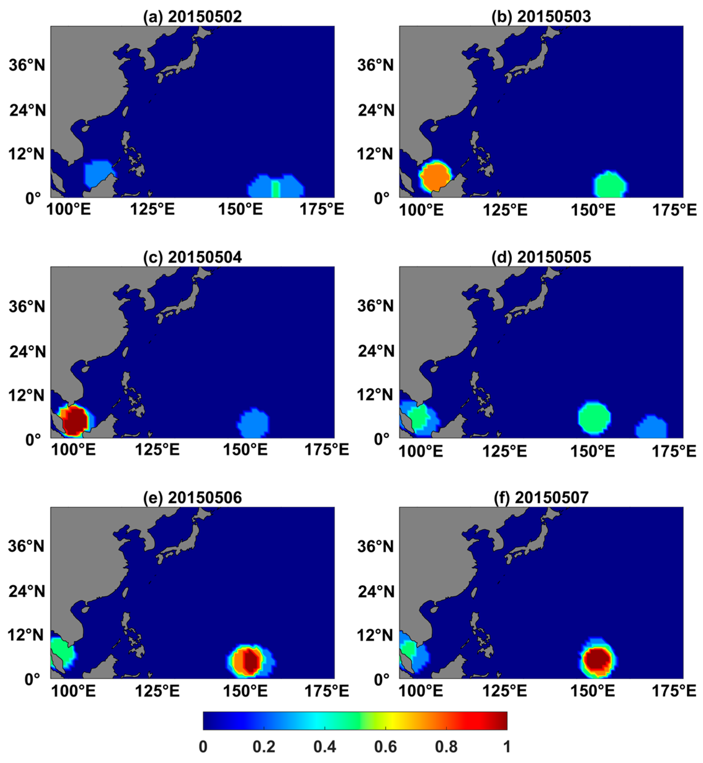
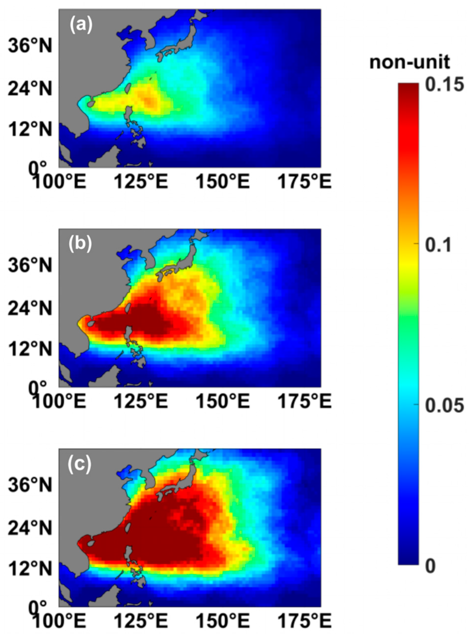
The choice of forecast time window can also influence the DBSS, and how to choose the time window is an interesting question. An excessively long time window is unfavorable for forecasting individual TCs [14,17], while a short time window can easily lead to inaccurate forecasting [15]. This experiment was conducted with forecast time windows of 1, 3, and 5 days, respectively. For the multi-day sliding forecast time window, the algorithm expands bidirectionally (both forward and backward in time). When processing the observational data, all TC positions within the extended 3-day (or 5-day) period were aggregated to compute the DTCP, though the word “daily” is not accurate when the forecast time window is 3 or 5 days. 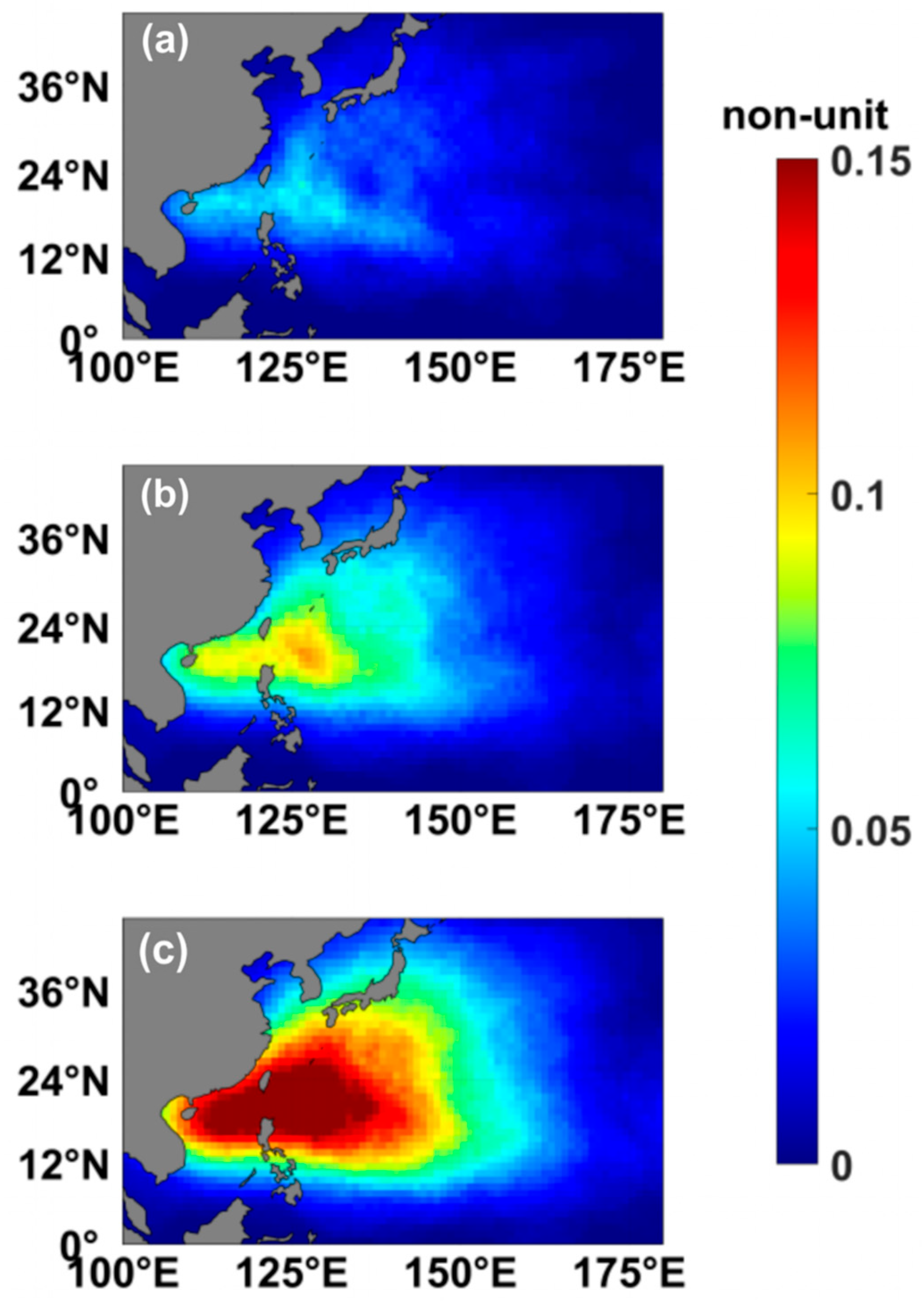As illustrated in Figure 4, extending the forecast time window led to an increase in the observed climatological DTCP, as it included TC occurrences across multiple days. To compute the model’s DTCP, the DTCP is first computed separately for each day, and the maximum DTCP across different days at the same grid point was selected as the final forecast DTCP.

It should be noted that when extending the forecast time window to 3 days, the first day (Day 1) and the last day (Day 30) cannot be expanded further backward or forward, respectively. Similarly, for a 5-day forecast time window, Days 1–2 and Days 29–30 cannot be extended beyond the available time range. Consequently, when applying a 3-day (or 5-day) forecast time window, the mean DBSS values for Day 1 and Day 30 (or Days 1–2 and Days 29–30) were excluded from the comparison.

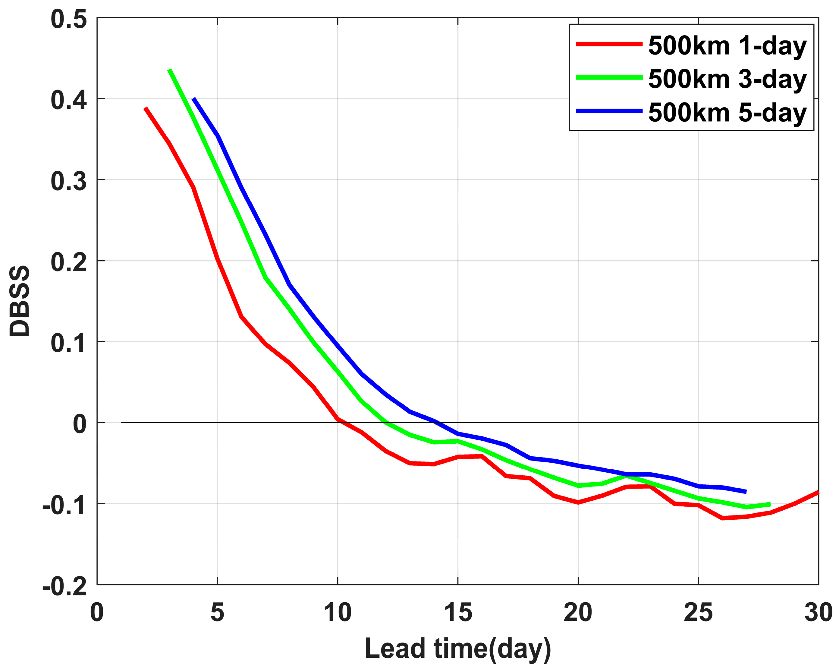
As shown in Figure 5, the mean DBSS of the ECMWF model increased with the extension of the forecast time window. The reason may have been that a longer forecast time window allowed for greater permissible errors in the model predictions, thereby leading to a higher mean DBSS. The increase of mean DBSS with a longer forecast time window is limited since the DBSS is the ratio of model forecast error and forecast error from a reference climate forecast (if the D term is ignored).

When the forecast time window was extended to 3 days, the mean DBSS dropped below 0 by day 12. Similarly, with a 5-day forecast time window, the mean DBSS fell below 0 by day 14. This result demonstrates that the DBSS did not change dramatically and exhibited robustness in response to variations in the forecast time window.

3.3. Test of TC Influence Radius

Similar to the selection of time windows, choosing the appropriate TC influence radius is crucial for evaluation. When the spatial range of forecast indicators are excessively broad, it is impossible to accurately locate TCs (such as ACE [18] or ‘box’ evaluation [19,20,21]), and overly specific forecast variables are also not suitable for the S2S scale (such as TC tracks [15]). In the definition of DTCP, the area within the TC influence radius is considered to be affected by the TC. The size of the TC influence radius can influence the calculation of DTCP. We examined the impact on mean DBSS by setting the TC influence radius to 300 km and 700 km, and compared the results with a TC influence radius of 500 km. As illustrated in Figure 6, the increase in the TC influence radius led to a larger area being affected by TC, consequently resulting in higher observed climatological DTCP.

Figure 7 shows the mean DBSS of the ECMWF model using different TC influence radius. The smallest DBSS occured within the 300 km radius, dropping below zero by day 9. The 700 km radius yielded a higher DBSS that fell below 0 by day 12. For the intermediate 500 km radius, the mean DBSS became negative on day 10. Consistent with the findings from the influence of forecast time window, the differences in mean DBSS among various TC influence radii remained relatively small. This behavior was as expected, because a larger TC influence radius accommodates greater positional errors in model forecasts. However, the expanded radius also introduces more false alarms as it covers larger areas where the TC may not actually occur. Consequently, while increasing the TC influence radius does moderately enhance the value of the DBSS, the enhancement is limited, demonstrating that the DBSS exhibits low sensitivity to variations in the TC influence radius.

3.4. Test of Brier Score for Reference Climate Forecast

Previous research conducted an analysis of the correction effect of term D, demonstrating that incorporating this term can effectively mitigate the negative bias in models with limited ensemble members [23,24]. However, in the application of Formula (1), $<\mathrm{B}\mathrm{S}>$ and $<{\mathrm{B}\mathrm{S}}_{\mathrm{C}\mathrm{L}}>$ were computed without distinguishing between event categories (i.e., TC occurrence and non-occurrence), which may have led to an overestimation of term D’s contribution to the DBSS calculation. In Formulas (3) and (4), $<{\mathrm{B}\mathrm{S}}_{\mathrm{C}\mathrm{L}}>$ can be derived either through theoretical calculation or estimated directly from model forecast samples, potentially yielding different DBSS values depending on the computation method. To investigate this sensitivity, we designed four experimental calculations: (1) using $<{\mathrm{B}\mathrm{S}}_{\mathrm{C}\mathrm{L}\_\mathrm{t}\mathrm{h}\mathrm{e}\mathrm{o}\mathrm{r}\mathrm{y}}>$ with D; (2) using $<{\mathrm{B}\mathrm{S}}_{\mathrm{C}\mathrm{L}\_\mathrm{t}\mathrm{h}\mathrm{e}\mathrm{o}\mathrm{r}\mathrm{y}}>$ without D; (3) using $<{\mathrm{B}\mathrm{S}}_{\mathrm{C}\mathrm{L}\_\mathrm{e}\mathrm{s}\mathrm{t}\mathrm{i}\mathrm{m}\mathrm{a}\mathrm{t}\mathrm{e}}>$ with D; and (4) using $<{\mathrm{B}\mathrm{S}}_{\mathrm{C}\mathrm{L}\_\mathrm{e}\mathrm{s}\mathrm{t}\mathrm{i}\mathrm{m}\mathrm{a}\mathrm{t}\mathrm{e}}>$ without D. This comparison allowed evaluation of DBSS’s sensitivity to different calculation methods of $<{\mathrm{B}\mathrm{S}}_{\mathrm{C}\mathrm{L}}>$ and the inclusion (or exclusion) of term D.

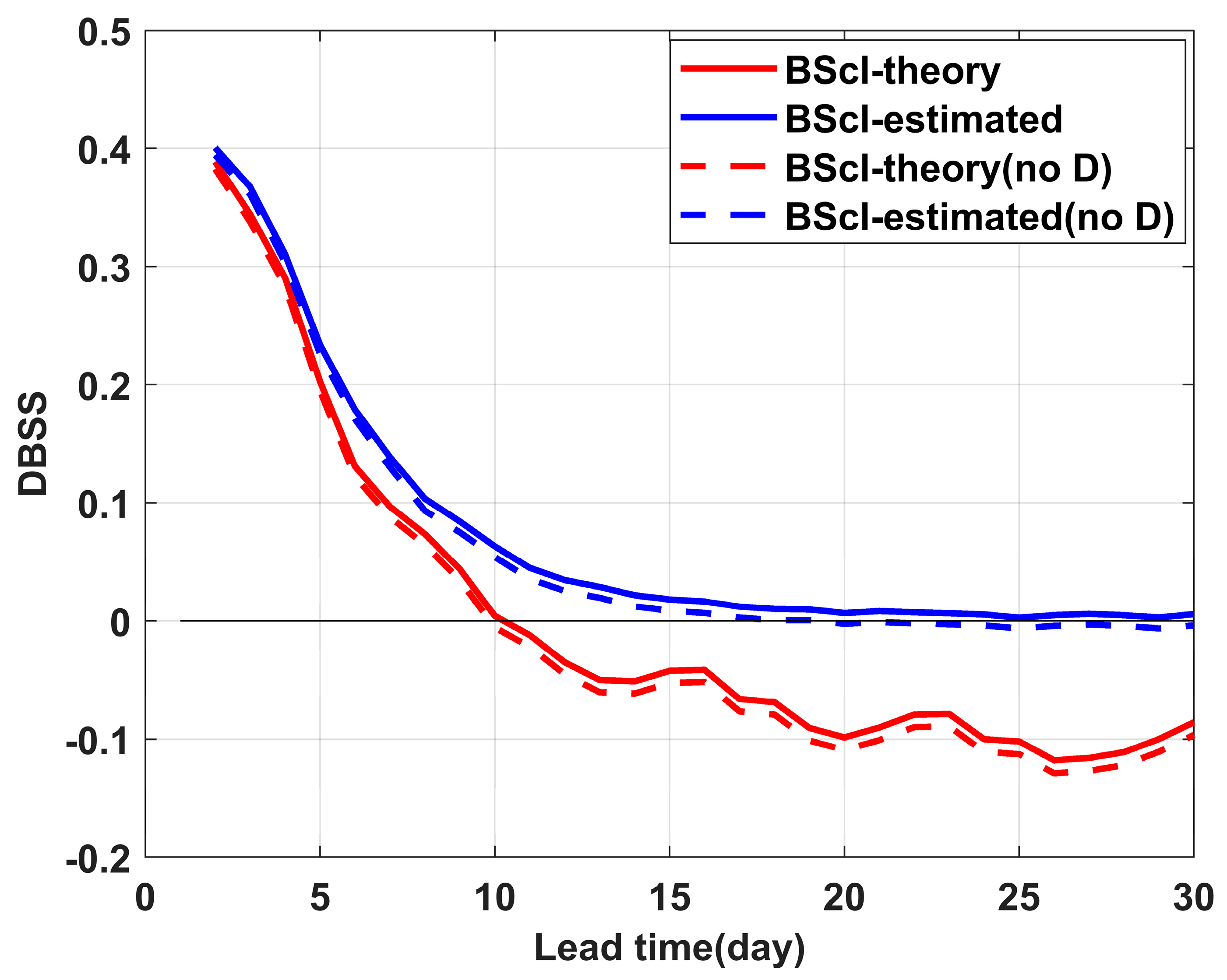
The experimental results presented in Figure 8 demonstrate that DBSSs computed using different $<{\mathrm{B}\mathrm{S}}_{\mathrm{C}\mathrm{L}}>$ methods remained nearly identical during the first 5 forecast days, but they began to diverge significantly after day 10. Notably, the mean DBSS based on $<{\mathrm{B}\mathrm{S}}_{\mathrm{C}\mathrm{L}\_\mathrm{e}\mathrm{s}\mathrm{t}\mathrm{i}\mathrm{m}\mathrm{a}\mathrm{t}\mathrm{e}}>$ approached zero after day 15, while that calculated using $<{\mathrm{B}\mathrm{S}}_{\mathrm{C}\mathrm{L}\_\mathrm{t}\mathrm{h}\mathrm{e}\mathrm{o}\mathrm{r}\mathrm{y}}>$ dropped below zero after day 10.

A distinct smoothing effect was observed in the mean DBSS curve when $<{\mathrm{B}\mathrm{S}}_{\mathrm{C}\mathrm{L}\_\mathrm{e}\mathrm{s}\mathrm{t}\mathrm{i}\mathrm{m}\mathrm{a}\mathrm{t}\mathrm{e}}>$ was employed, compared with the $<{\mathrm{B}\mathrm{S}}_{\mathrm{C}\mathrm{L}\_\mathrm{t}\mathrm{h}\mathrm{e}\mathrm{o}\mathrm{r}\mathrm{y}}>$ results. This smoothing is likely to be because $<{\mathrm{B}\mathrm{S}}_{\mathrm{C}\mathrm{L}\_\mathrm{e}\mathrm{s}\mathrm{t}\mathrm{i}\mathrm{m}\mathrm{a}\mathrm{t}\mathrm{e}}>$ was derived from forecast samples where the sample size was inherently linked to the frequency of forecasts. This relationship between sample size and forecast frequency may have introduced fluctuations in the $<{\mathrm{B}\mathrm{S}}_{\mathrm{C}\mathrm{L}}>$ calculations. However, when both $<{\mathrm{B}\mathrm{S}}_{\mathrm{C}\mathrm{L}\_\mathrm{e}\mathrm{s}\mathrm{t}\mathrm{i}\mathrm{m}\mathrm{a}\mathrm{t}\mathrm{e}}>$ and $<\mathrm{B}\mathrm{S}>$ were computed based on model forecast frequencies, these fluctuations tended to cancel each other out. Further investigation into the effects of forecast frequency and sample size will be presented in a subsequent case study. When different models are involved in the evaluation, using an estimated Brier score for reference climate forecast is not appropriate, since the practice introduces a different Brier score for the reference climate forecast.

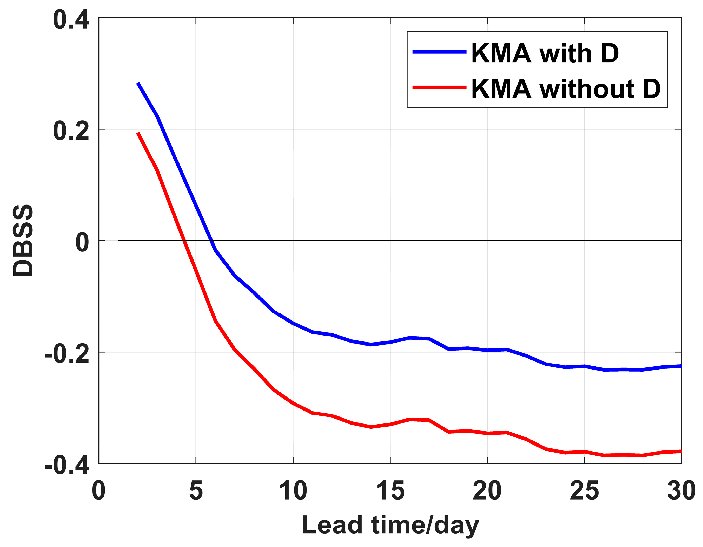
Figure 8 illustrates that including the D-term caused relatively minor variations in the mean DBSS. As indicated in Table 1, this limited impact can be attributed to the ECMWF model’s substantial ensemble size of 51 members, which resulted in a considerably small magnitude of the D correction term computed from Formula (5). To further examine the impact of D in models with smaller ensemble sizes, we conducted experiments using the KMA model, which operates with only four ensemble members. Figure 9 demonstrates a pronounced enhancement in mean DBSS following the implementation of the D correction term in the KMA model. This analysis clearly indicates that the D term plays a crucial role in models with small numbers of ensemble members, effectively correcting negative skill score biases, while its contribution becomes less significant in models with large ensemble sizes such as the ECMWF model.

Previous studies [19,23,24,26] emphasized the fundamental importance of ensemble size in evaluating model forecast skill. The inclusion of the D correction term in the assessment of forecasting skill is particularly valuable, especially for operational models with few ensemble members.

3.5. Test of Forecast Frequency

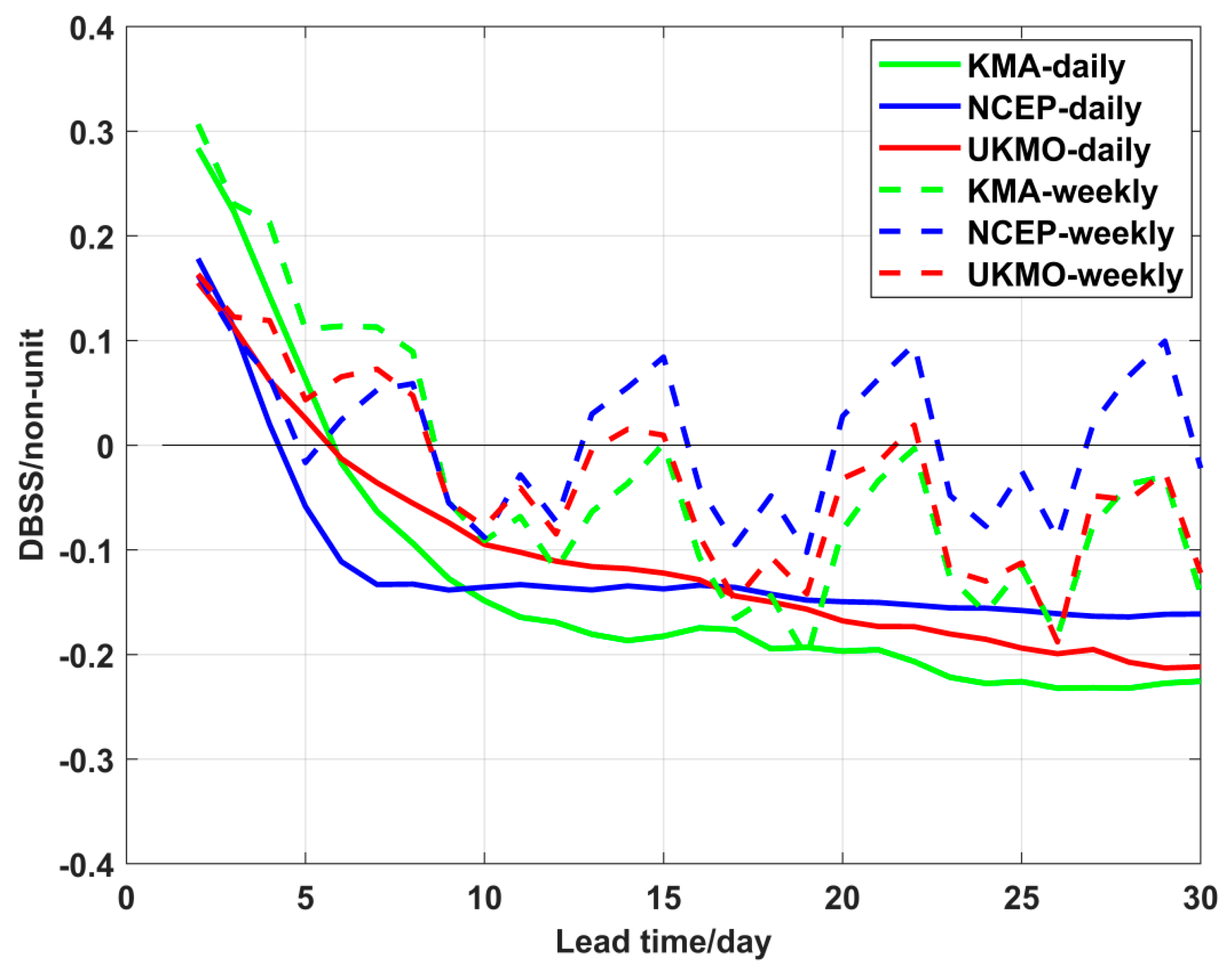
In Section 3.4, we mentioned the impact of forecast sample size on DBSS. To further investigate its influence, we conducted experiments by modifying the frequency of forecasts to alter the sample size. We selected three daily forecast models (KMA, NCEP, and UKMO) from the S2S real-time database and artificially changed their forecast frequency from daily to weekly, thereby creating three hypothetical models.

Compared with the mean DBSS of the original daily forecast models, their weekly forecast counterparts revealed pronounced periodic oscillations in mean DBSS (Figure 10). This phenomenon arose from reduced forecast sample sizes leading to increased uncertainty. These results clearly demonstrate that variations in the sample size of forecasts significantly affect DBSS. Consequently, when evaluating models’ forecasting skill, careful consideration of sample sizes is essential to ensure reliable assessment.

It is worth noting that although our experiments specifically focused on the DTCP and DBSS framework, the findings possess broader applicability to other TC probability forecasting evaluation frameworks. For instance, the ‘Box’ approach employed by earlier researchers [18,19,20,21] shares conceptual similarities with our TC influence radius definition, while the 3-day sliding window [16] closely resembles our forecast time window methodology. The quantitative findings of our research might be different for other models and other TC basins, as indicated by a research focusing on the predictability range of ensemble forecasts [35]. This study provides some guidance for evaluating S2S TC forecasts and establishes a foundation for future global assessments of S2S TC forecast skill.

4. Discussion and Conclusions

Currently, there is no universally accepted standard for evaluating S2S TC forecasts. Several probabilistic variables have been proposed, including daily tropical cyclone probability (DTCP) and the debiased Brier skill score (DBSS) framework. In this study, we systematically examined the influence of several important factors using DTCP as the forecast variable and DBSS as the forecasting skill score metric. Through separate sensitivity tests, we demonstrated that while modifications to the evaluation region, forecast time window, and TC influence radius altered spatially averaged DBSS values, their overall impacts remained consistent and relatively minor. However, the use of estimated Brier score for reference climate forecasts introduces notable variability due to the limited sample sizes—a crucial consideration when evaluating models’ forecasting skill.

Based on the results presented in Section 3, we recommend the following for multi-model evaluation on S2S scale. (1) The theoretical Brier score should be used for reference climate forecasts to ensure fair comparisons between different models. (2) The correction term D should be applied to mitigate negative biases while evaluating models with small ensemble sizes. (3) While expanding either the forecast time window or TC influence radius may improve forecasting skill scores, these adjustments simultaneously reduce spatial precision in TC localization. Therefore, these key parameters should be carefully selected based on specific operational requirements. These recommendations provide standardized evaluation criteria while maintaining the flexibility necessary for diverse operational applications.

The DTCP and DBSS framework evaluated here transcends the WNP focus of this study, offering a scalable template for evaluation of global S2S TC forecasting. By analyzing factors such as ensemble size, forecast frequency, and reference climatology, this work bridges gaps between research and operational implementation. Moreover, our results underscore the potential of S2S forecasts to enhance early warning systems and adaptive management strategies; for example, adjusting the forecast time window and TC influence radius introduces greater flexibility into predictions. We also prove their robustness for operational applications.

As climate change amplifies TC risks, the ability to predict TC activity weeks in advance becomes indispensable for safeguarding lives and economies. Future research could extend this framework to other basins and explore couplings with oceanic and atmospheric drivers (e.g., MJO, ENSO) to further enhance predictions. This study refines the technical evaluation of S2S TC forecasts and by clarifying the impacts of evaluation choices, we pave the way for more credible, actionable, and globally relevant S2S predictions, ultimately contributing to resilience in the face of growing threats from tropical cyclones.