Sea Clutter Suppression Method Based on Correlation Features

Abstract

Radar target detection in a sea clutter environment is of significant importance in both civilian and military applications, with the detection of small maneuvering targets being particularly challenging. To address this issue, this paper introduces the autocorrelation characteristics of sea clutter into orthogonal projection operations to suppress sea clutter and enhance the detection capability of small maneuvering targets on the sea surface. The proposed method first generates speckle components that are consistent with the correlation characteristics of the observed sea clutter. Then, it uses these speckle components to derive the feature subspace of the sea clutter and applies this subspace in an orthogonal projection suppression algorithm, thereby achieving effective suppression of the sea clutter. This method does not rely on the covariance matrix estimation of sea clutter from reference cells but instead directly utilizes the autocorrelation characteristics of the observed sea clutter data to obtain the feature subspace, making it more adaptable to different environments. Simulation and experimental results demonstrate that this method significantly suppresses sea clutter and effectively improves the performance of target detection on the sea surface.

1. Introduction

As the demand for real-time monitoring and precise detection of maritime targets increases, the ability of radar to quickly and reliably detect small maneuvering targets on the sea surface (such as small boats, divers, low-flying aircraft, etc.) has become increasingly important [1,2]. However, due to the influence of surface motion in the sea, sea clutter exhibits non-homogeneous, non-Gaussian, and non-stationary characteristics, causing interference with sea surface targets in both the time and frequency domains. Current research on small sea surface target detection mainly focuses on two aspects: one is the study of sea clutter suppression methods, and the other is the development of sea target detection algorithms. Since sea clutter suppression is a prerequisite for effective target detection, it is of greater importance.

At present, approaches for sea clutter suppression include time-domain cancellation methods, wavelet transform techniques, deep learning-based approaches, space-time adaptive processing (STAP), and subspace-based methods. Time-domain cancellation methods suppress sea clutter by constructing a cancellation signal from measured clutter data and subtracting it from the observed signal. A typical example is the Moving Target Indication (MTI) technique, which can only filter out clutter near zero Doppler frequency and is incapable of adapting to Doppler shifts in sea clutter [3,4]. To achieve more accurate suppression, some studies generate cancellation signals based on estimated sea clutter parameters obtained from measurements [5,6,7]. However, these methods heavily rely on the precise estimation of clutter characteristics, and any deviation in the estimated parameters may weaken the target echo features, resulting in suboptimal clutter suppression performance. The wavelet transform method separates sea clutter from target signals in the wavelet domain and removes clutter using thresholding, but it depends on selecting an appropriate basis function and may distort the phase information of the received signal [8]. With the development and application of deep learning [9,10], researchers have proposed new sea clutter suppression methods from the perspective of image processing [11,12]. In addition, techniques such as multi-label feature selection and pixel-based feature selection can be applied to sea clutter suppression [13,14,15,16]. Although these methods perform well in some cases, they still face issues such as model complexity and poor generalization, which limit their widespread application. Space-time adaptive processing (STAP) can effectively utilize multi-domain information such as spatial, Doppler, and range data to suppress sea clutter [17,18]. Although this method provides performance improvements to varying degrees, STAP is mainly suited for airborne radar systems and involves high computational complexity. In contrast, subspace-based sea clutter suppression algorithms have been widely applied in radar target detection due to their strong target feature extraction capabilities, lower computational complexity, and better engineering feasibility.

Subspace methods typically decompose the echo signal into the sea clutter feature subspace and the signal feature subspace. The singular values corresponding to the sea clutter feature subspace are set to zero, and the signal is then reconstructed to achieve sea clutter suppression [19]. Reference [20] proposed a sea clutter suppression algorithm that combines singular value decomposition (SVD) and fractional Fourier transform (FrFT). However, since the number of singular values corresponding to the sea clutter feature subspace and the signal order are typically unknown, this method relies on prior knowledge of the sea clutter, making it difficult to adaptively filter out the clutter. Building on subspace-based ideas, Yang et al. proposed an orthogonal projection-based constant false alarm rate (CFAR) detection algorithm [21], which considers the similarity of radar echo signals from adjacent range cells. This method constructs an orthogonal projection operator in the projection space to suppress sea clutter. The aforementioned subspace methods often rely on neighboring reference cells to estimate the sea clutter covariance matrix, assuming that the sea clutter is homogeneous—i.e., the backscatter in each range bin follows the same statistical distribution. However, in practical applications, the training samples from adjacent range bins do not always satisfy the assumption of independent and identically distributed (i.i.d.) data [22]. As a result, the sea clutter covariance matrix estimation may be inaccurate, which in turn affects the effectiveness of clutter suppression [23,24]. To address this issue, Reference [25] leveraged the fact that sea clutter exhibits different texture features in different polarization channels and proposed a maximum likelihood (ML) criterion-based covariance matrix method. Reference [26] applied an over-symmetry method for covariance matrix estimation, reducing reliance on training sample data. Reference [27] used prior information to improve the accuracy of covariance matrix estimation, resulting in a fully adaptive radar target coherent detector. Reference [28] proposed a covariance matrix estimation method based on hidden Markov models and compound Gaussian models.

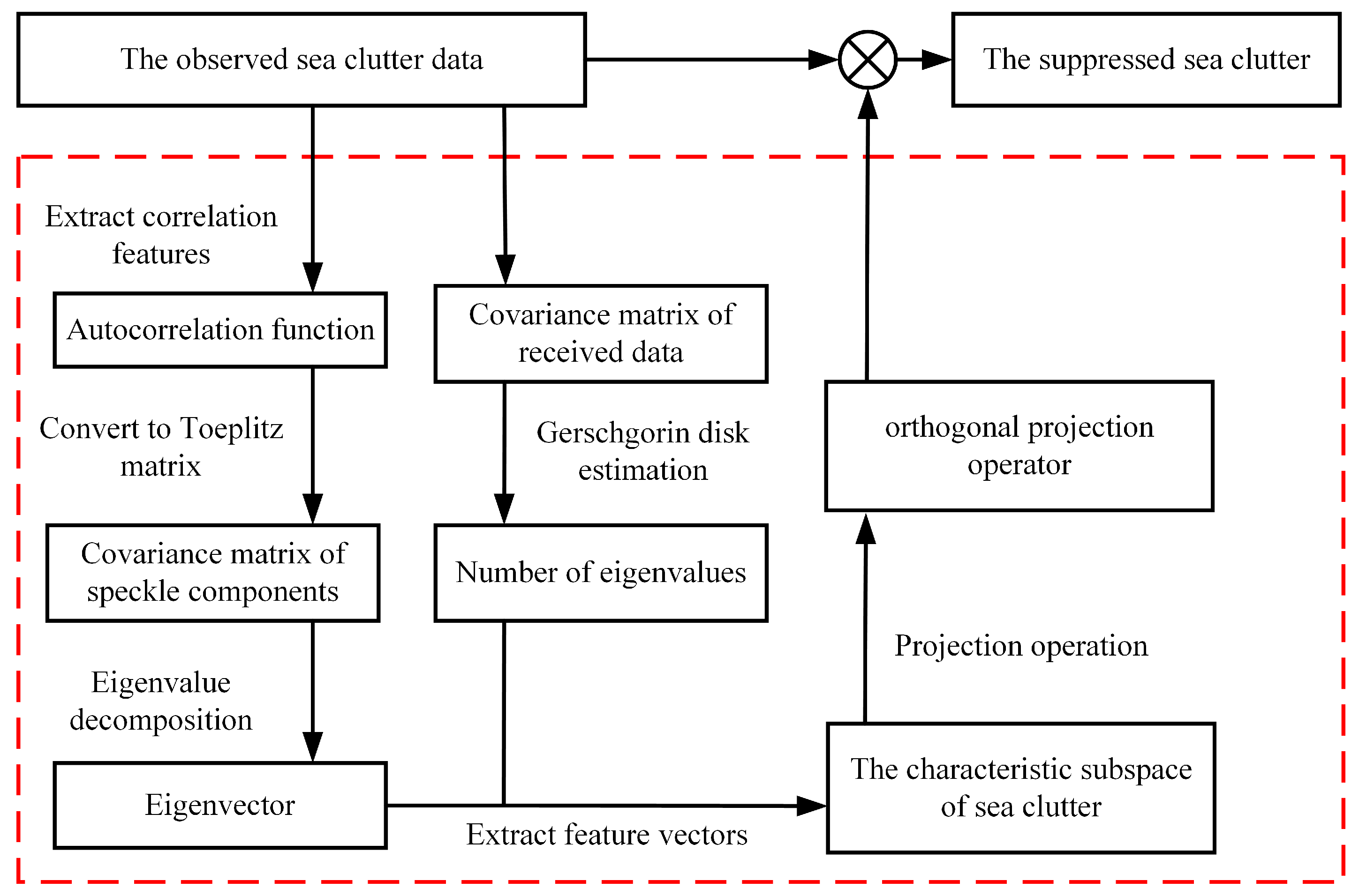
To address the challenges faced by subspace methods in practical applications, this paper proposes an orthogonal projection-based sea clutter suppression method that constructs the covariance matrix using speckle components. The method first computes the autocorrelation function of sea clutter and utilizes this function to generate speckle components. These speckle components are then used to construct the required covariance matrix. Finally, the original signal is orthogonally projected onto the sea clutter feature subspace to achieve clutter suppression. Unlike traditional methods, the proposed approach directly constructs the sea clutter covariance matrix from the received data, without relying on training data from adjacent cells, thereby avoiding inaccuracies in covariance matrix estimation. This innovation not only simplifies the sea clutter suppression process but also provides new insights and methods for related fields. The main contributions of this paper are as follows:

(1)

We propose a novel method to construct the covariance matrix of speckle components using the autocorrelation function of observed sea clutter, enabling the formation of a clutter feature subspace for suppression. Based on this subspace, an orthogonal projection operator is derived and applied to effectively suppress sea clutter. The feasibility of using speckle components for clutter suppression is analyzed, providing a new perspective for subspace construction in nonstationary clutter environments.

(2)

We prove the relationship between the eigenvectors of the sea clutter covariance matrix and the eigenvectors of the texture component covariance matrix. The conclusion drawn is: “The magnitude of the eigenvalues of the sea clutter covariance matrix is mainly determined by the texture components, while the eigenvectors are primarily determined by the speckle components”. This finding provides theoretical support for the sea clutter suppression method proposed in this paper.

(3)

Traditional methods often estimate the sea clutter covariance matrix using adjacent reference cells around the cell under test. However, due to inconsistencies in the clutter spectral characteristics between the test cell and the reference cells, the covariance matrix estimation can suffer from significant errors. The proposed sea clutter suppression method does not rely on reference cells to construct the covariance matrix. Instead, it generates speckle components based on the autocorrelation characteristics of the observed sea clutter data and uses these components to suppress the clutter. This approach offers a novel perspective for sea clutter suppression.

Table 1. Comparison of the proposed method with existing sea clutter suppression techniques.

Method Type	Advantages	Disadvantages	Relative Advantages of Proposed Method
Deep Learning Methods	Automatic feature extraction; performs well in some scenarios	Complex models, high demand for training data, poor generalization	No need for training data; simple algorithm; strong adaptability
STAP	Capable of handling non-homogeneous clutter; strong performance	High computational complexity; suitable for airborne radar only	Low computational cost; suitable for real-time processing in ground-based radar
Wavelet Transform Methods	Can distinguish different frequency components	Depends on wavelet basis selection; may distort phase information	More robust due to being based on physical modeling
MTI	Good real-time performance; simple structure	Only suppresses static or low-speed clutter; ineffective for Doppler-shifted clutter	Capable of adapting to clutter Doppler shifts; stronger suppression ability
Orthogonal Projection Algorithm [21]	Can suppress similar clutter structures	Inaccurate covariance estimation under non-homogeneous sea clutter	Constructs projection operator directly from observed data; avoids reference cell errors

presents the main differences and advantages between the proposed method and deep learning, STAP, wavelet-based methods, and MTI, as well as existing orthogonal projection algorithms.

The structure of the rest of the paper is arranged as follows: Section 2 describes the problems that need to be addressed in sea clutter suppression. Section 3 presents the generation of speckle components using the sea clutter autocorrelation function. Section 4 provides a detailed description of the sea clutter suppression method proposed in this paper. Section 5 presents the simulation experiments and validation of the proposed method. Finally, Section 6 provides a conclusion and summary of the paper.

2. Problem Description

For pulse-Doppler radar, in the case where sea clutter dominates, the presence of a target in the echo signal received from the detection cell can be represented by the following binary hypothesis test:

$$\left\{\begin{array}{c}{H}_0:x=c\\ H_1:x=c+ap\end{array}\right.$$

(1)

Here, the null hypothesis $H_0$ indicates that there is no target signal in the data to be detected, while the alternative hypothesis $H_1$ indicates that there is a target signal in the data to be detected. x is the observed signal, c is the sea clutter signal, a represents the target amplitude, and p is the steering vector of the target.

To improve the probability of target detection, the most direct approach is to reduce the impact of sea clutter. To achieve this, it is necessary to thoroughly study the sea clutter model and identify effective suppression methods. According to the compound Gaussian model, sea clutter consists of two components: the texture component and the speckle component. The texture component primarily reflects the amplitude characteristics of sea clutter, while the speckle component mainly represents its correlation characteristics. The speckle component consists of echoes from a large number of independent basic scatterers and follows a zero-mean complex Gaussian distribution with fast variations. In contrast, the texture component reflects the power level of the radar illumination area and changes relatively slowly. During a period of coherent integration, when the observation time is only a few microseconds, the compound Gaussian model simplifies to the Spherically Invariant Random Vector (SIRV) model [29,30], i.e.:

$$c=\sqrt{\tau }\eta ,\tau \sim p\left(\tau \right),\eta \sim CN(0,\mathbf{M})$$

(2)

In the equation, c represents the sea clutter data, $\eta$ denotes the speckle component, $\tau$ denotes the texture component, $CN(0,\mathbf{M})$ is a complex Gaussian random vector with zero mean and covariance matrix $\mathbf{M}$, and $p\left(\tau \right)$ is the probability density function of the texture component $\tau$.

The amplitude distribution of sea clutter exhibits non-Gaussianity, primarily due to the texture components. Given the texture component, the conditional probability of the sea clutter amplitude is:

$$f\left(c\right|\tau )={\displaystyle \frac{1}{{\left(\pi \tau \right)}^m\left|\mathbf{M}\right|}}exp(-{\displaystyle \frac{c^H{\mathbf{M}}^{-1}c}{\tau }})$$

(3)

Here, $|·|$ represents the matrix determinant, $\mathbf{M}$ is the covariance matrix that the speckle component follows, and the statistical average of $f\left(c\right|\tau )$ with respect to gives the probability density function of c:

$$f\left(c\right)={\int }_0^{\infty }f\left(c\right|\tau )p\left(\tau \right)d\tau$$

(4)

Here, $p\left(\tau \right)$ represents the probability density function of the texture component.

Since the amplitude of the texture component is a random variable that follows a specific probability density function, it, together with the speckle component that follows a Rayleigh distribution, jointly determines the amplitude characteristics of sea clutter [31]. As the range cell changes, the sea clutter power fluctuates, causing the texture component to also fluctuate. Therefore, in different reference cells, the texture components typically vary, making it difficult to accurately estimate the texture component of the cell under test. This variability increases the difficulty of distinguishing sea clutter based on amplitude characteristics, making it hard to effectively suppress sea clutter using the texture component alone. In contrast, the correlation characteristics of the speckle component contain Doppler information and phase difference information between the real and imaginary parts of the signal, and the correlation characteristics of sea clutter are relatively stable [32]. Therefore, utilizing speckle components offers a significant advantage in sea clutter suppression.

3. Constructing Speckle Components Based on Correlation Characteristics

Sea clutter correlation refers to the correlation characteristics exhibited between radar signal pulses within range resolution cells, reflecting the surface fluctuations of the sea. The autocorrelation function is obtained by summing the product of the signal’s value at each time point with its value after a certain delay [33]. For sea clutter data, the autocorrelation function gradually converges to zero as the number of time intervals increases and exhibits a specific shape, making it a useful basis for identifying sea clutter. This section presents a method for extracting sea clutter features, aiming to provide a detailed description of the correlation characteristics of sea clutter.

Assuming that the sea clutter signal c satisfies the generalized stationary property, the correlation between different time points primarily depends on the time delay and is independent of the specific time points. By averaging the autocorrelation functions of all range cells in the sample, an approximate expression for the autocorrelation function can be obtained:

$$\tilde{r}\left(k\right)={\displaystyle \frac{1}{M}}\sum _{m=1}^M\left[{\displaystyle \frac{\frac{1}{N-k}{\sum }_{n=0}^{N-k-1}{c}_{m,n}{c}_{m,n+k}}{\frac{1}{N}{\sum }_{n=0}^{N-1}{\left|c_{m,n}\right|}^2}}\right]$$

(5)

In the equation, M represents the number of range cells in the sample, N represents the number of pulses in the sample, $c_{m,n}$ denotes the echo signal of the m-th range cell in the n-th pulse, and k represents the pulse interval number.

It should be noted that even if a target exists in the observed sea clutter data, its impact on the autocorrelation function is not significant. This is because the aforementioned autocorrelation function is obtained by averaging the correlation across all range cells, and in sea clutter data that include a large number of range cells, the proportion of the target is minimal, so its effect can be neglected. Therefore, even in the presence of a target, the resulting sea clutter autocorrelation function can still accurately reflect the correlation of sea clutter in the observed sample.

Sea clutter signals typically exhibit strong temporal variability, and the autocorrelation function is used to describe the similarity between the signal at different time points. Therefore, as the time interval increases, the autocorrelation function of the sea clutter data gradually decreases, the similarity between the signals weakens, and it eventually approaches zero. The number of time intervals K at which the autocorrelation function converges to zero can be calculated using the following formula:

$$K=\min \left\{k:|\tilde{r}\left(k\right)|<\epsilon \right\}$$

(6)

Here, $\epsilon$ represents a threshold close to zero.

By setting the autocorrelation function value to zero for time intervals greater than K, the autocorrelation matrix formed by the autocorrelation function of the sea clutter data becomes a Toeplitz matrix, which can be expressed as:

$$\mathbf{C}=\left[\begin{array}{cccccc}\tilde{r}\left(0\right)& \tilde{r}\left(1\right)& \dots & \tilde{r}\left(K\right)& \dots & 0\\ \tilde{r}\left(1\right)& \tilde{r}\left(0\right)& \dots & \tilde{r}(K-1)& \dots & 0\\ ⋮& ⋮& \ddots & ⋮& & ⋮\\ \tilde{r}\left(K\right)& \tilde{r}(K-1)& \dots & \tilde{r}\left(0\right)& \dots & ⋮\\ ⋮& ⋮& & ⋮& \ddots & ⋮\\ 0& 0& \dots & \dots & \dots & \tilde{r}\left(0\right)\end{array}\right]$$

(7)

According to the SIRP theory, the speckle component originates from the radar echoes of a large number of basic scatterers, so its characteristics are not affected by the amplitude distribution [34]. Due to the excellent property of the Gaussian distribution, which retains its Gaussian nature after linear transformation, we choose the Gaussian distribution as the starting sample to generate the correlated clutter samples.

Let ${\mathbf{W}}_I$ and ${\mathbf{W}}_Q$ be M × N Gaussian white noise matrices. ${\mathbf{W}}_I$ and ${\mathbf{W}}_Q$ together form a complex Gaussian white noise matrix:

$$\mathbf{W}={\mathbf{W}}_1+j·{\mathbf{W}}_Q$$

(8)

We need to transform the complex Gaussian white noise matrix into a colored noise matrix with given correlation characteristics, thereby generating a speckle component matrix that reflects the correlation information of sea clutter. Since the Cholesky decomposition can introduce autocorrelation characteristics into independent and identically distributed white noise, it can also be used to generate a complex Gaussian white noise matrix with a specific autocorrelation structure [35]. The Cholesky decomposition of the autocorrelation matrix $\mathbf{C}$ is:

$$\mathbf{C}=\mathbf{L}{\mathbf{L}}^H$$

(9)

Here, $\mathbf{L}$ is the lower triangular matrix obtained from the Cholesky decomposition of $\mathbf{C}$.

Multiplying the complex white noise matrix by the matrix $\mathbf{L}$ obtained from the Cholesky decomposition gives a colored noise matrix with the desired correlation characteristics.

$$\mathit{\eta }=\mathbf{W}\mathbf{L}$$

(10)

The covariance matrix of the speckle component can be approximately expressed as:

$$\mathbf{M}=\mathit{\eta }{\mathit{\eta }}^H=\mathbf{L}\mathbf{W}{\mathbf{W}}^H{\mathbf{L}}^H=\mathbf{C}$$

(11)

Through derivation, we find that the covariance matrix of the speckle components can be expressed using the autocorrelation matrix of the sea clutter.

4. Sea Clutter Suppression Algorithm Based on Correlation

The sea clutter received by the receiver is typically composed of sea surface echoes and radar thermal noise [36]. The correlation characteristics of sea clutter are mainly determined by the sea surface echoes, and the sea surface echoes account for a larger proportion compared to thermal noise. Therefore, the eigenvectors corresponding to the large eigenvalues in the covariance matrix of the sea clutter data form the feature subspace of the sea clutter. Accurately selecting the feature subspace of the sea clutter is key to improving the performance of sea clutter suppression. To this end, this section uses the speckle components to extract the feature subspace of the sea clutter and applies this feature subspace to the orthogonal projection method for effective sea clutter suppression.

4.1. Determining the Subspace of Sea Clutter

4.1.1. The Relationship Between the Sea Clutter Covariance Matrix and the Speckle Component Covariance Matrix

According to the compound Gaussian model, the texture component of sea clutter is modeled as a random variable following a specific distribution, while the speckle component is represented as a complex Gaussian random vector characterized by a certain covariance matrix. We assume that the sea clutter data for the i-th pulse within a coherent processing interval (CPI) are given by:

$${\mathbf{c}}_i={\mathit{\mu }}_i{\mathit{\eta }}_i$$

(12)

Here, ${\mathit{\mu }}_i$ denotes the vector formed by taking the square root of the texture component values pointwise along the range dimension for the i-th pulse. ${\mathit{\eta }}_i$ represents the complex vector corresponding to the speckle component along the range dimension for the i-th pulse. Then, the elements of the sea clutter covariance matrix $\mathbf{R}$ within a coherent processing interval (CPI) can be expressed as:

$${\mathbf{R}}_{ij}={\left({\mathit{\mu }}_i{\mathit{\eta }}_i\right)}^H\left({\mathit{\mu }}_j{\mathit{\eta }}_j\right)={\mathit{\mu }}_i^H{\mathit{\mu }}_j{\mathit{\eta }}_i^H{\mathit{\eta }}_j$$

(13)

where i and j denote the i-th and j-th pulses, respectively.

Therefore, the covariance matrix $\mathbf{R}$ of the sea clutter can be expressed as:

$$\mathbf{R}=\left[\begin{array}{cccc}{\mathit{\mu }}_1^H{\mathit{\mu }}_1& {\mathit{\mu }}_1^H{\mathit{\mu }}_2& \dots & {\mathit{\mu }}_1^H{\mathit{\mu }}_N\\ {\mathit{\mu }}_2^H{\mathit{\mu }}_1& {\mathit{\mu }}_2^H{\mathit{\mu }}_2& \dots & {\mathit{\mu }}_2^H{\mathit{\mu }}_N\\ ⋮& ⋮& \ddots & ⋮\\ {\mathit{\mu }}_N^H{\mathit{\mu }}_1& {\mathit{\mu }}_N^H{\mathit{\mu }}_2& \dots & {\mathit{\mu }}_N^H{\mathit{\mu }}_N\end{array}\right]\mathbf{M}$$

(14)

Here, ⊙ represents the Hadamard product, and $\mathbf{M}$ is the covariance matrix of the speckle component.

Theorem 1. 

The magnitude of the eigenvalues of the sea clutter covariance matrix is primarily determined by the texture component, while the eigenvectors are mainly determined by the speckle component.

Proof. 

Perform an eigenvalue decomposition of the covariance matrix of the speckle components. The covariance matrix, eigenvalues, and eigenvectors of the speckle components satisfy the following relationship:

$$\mathbf{M}\mathbf{U}=\mathbf{U}\mathbf{\Sigma }$$

(15)

Here, $\mathbf{\Sigma }=diag\left({\lambda }_1,{\lambda }_2,\cdots ,{\lambda }_N\right)$ is the diagonal matrix composed of the eigenvalues of $\mathbf{M}$, and $\mathbf{U}=\left[u_1,u_2,\cdots ,u_N\right]$ is the matrix composed of the eigenvectors of $\mathbf{M}$.

Then, multiply the covariance matrix $\mathbf{R}$ of the sea clutter by the matrix $\mathbf{U}$ composed of the eigenvectors of the texture component, and perform the following derivation:

$$\begin{array}{c}\hfill \mathbf{R}=\left[\begin{array}{cccc}{\mathit{\mu }}_1^H{\mathit{\mu }}_1& {\mathit{\mu }}_1^H{\mathit{\mu }}_2& \dots & {\mathit{\mu }}_1^H{\mathit{\mu }}_N\\ {\mathit{\mu }}_2^H{\mathit{\mu }}_1& {\mathit{\mu }}_2^H{\mathit{\mu }}_2& \dots & {\mathit{\mu }}_2^H{\mathit{\mu }}_N\\ ⋮& ⋮& \ddots & ⋮\\ {\mathit{\mu }}_N^H{\mathit{\mu }}_1& {\mathit{\mu }}_N^H{\mathit{\mu }}_2& \dots & {\mathit{\mu }}_N^H{\mathit{\mu }}_N\end{array}\right]\odot \mathbf{M}\mathbf{U}=\left[\begin{array}{cccc}{\mathit{\mu }}_1^H{\mathit{\mu }}_1& {\mathit{\mu }}_1^H{\mathit{\mu }}_2& \dots & {\mathit{\mu }}_1^H{\mathit{\mu }}_N\\ {\mathit{\mu }}_2^H{\mathit{\mu }}_1& {\mathit{\mu }}_2^H{\mathit{\mu }}_2& \dots & {\mathit{\mu }}_2^H{\mathit{\mu }}_N\\ ⋮& ⋮& \ddots & ⋮\\ {\mathit{\mu }}_N^H{\mathit{\mu }}_1& {\mathit{\mu }}_N^H{\mathit{\mu }}_2& \dots & {\mathit{\mu }}_N^H{\mathit{\mu }}_N\end{array}\right]\odot \mathbf{U}\mathbf{\Sigma }\\ \hfill =\mathbf{U}\left[\begin{array}{cccc}{\mathit{\mu }}_1^H{\mathit{\mu }}_1{\mathit{\lambda }}_1^H& 0& \dots & 0\\ 0& {\mathit{\mu }}_2^H{\mathit{\mu }}_2{\mathit{\lambda }}_2^H& \dots & 0\\ ⋮& ⋮& \ddots & ⋮\\ 0& 0& \dots & {\mathit{\mu }}_N^H{\mathit{\mu }}_N{\mathit{\lambda }}_N^H\end{array}\right]=\mathbf{U}\widehat{\mathit{\Sigma }}\end{array}$$

(16)

At this point, $\widehat{\mathit{\Sigma }}=diag({\mathit{\mu }}_1^H{\mathit{\mu }}_1{\mathit{\lambda }}_1^H,{\mathit{\mu }}_2^H{\mathit{\mu }}_2{\mathit{\lambda }}_2^H,\cdots ,{\mathit{\mu }}_N^H{\mathit{\mu }}_N{\mathit{\lambda }}_N^H)$ is the diagonal matrix composed of the eigenvalues of $\mathbf{R}$. We find that the eigenvectors of the covariance matrix $\mathbf{R}$ are the same as the eigenvectors of the covariance matrix of the speckle component.

Therefore, it can be concluded that the eigenvalues of the sea clutter covariance matrix are primarily determined by the texture component, while the eigenvectors are mainly determined by the speckle component. □

4.1.2. Obtaining the Sea Clutter Subspace Using the Speckle Component Covariance Matrix

The sea clutter covariance matrix describes the correlation of and variance in sea clutter data in different dimensions. The matrix $\mathbf{U}$ can be considered as the direction of the components of the sea clutter covariance matrix, directly reflecting the correlation characteristics of the data along these directions, while $\widehat{\mathit{\Sigma }}$ represents the variance in the corresponding directions. The amplitude information of the sea clutter is contained in $\widehat{\mathit{\Sigma }}$, while $\mathbf{U}$ only contains the correlation information of the sea clutter.

Since the speckle component shares the same eigenvectors as the covariance matrix of the sea clutter, the eigenvectors corresponding to the large eigenvalues in the speckle component’s covariance matrix can also form the subspace of the sea clutter. However, the eigenvalues of the speckle component and the sea clutter covariance matrix are not identical, and the number of eigenvectors determined solely by the speckle component is inaccurate. To address this issue, we utilize the received data to obtain the sea clutter covariance matrix and apply the Gerschgorin disk estimation (GDE) method [37] to determine the number of eigenvectors corresponding to the sea surface echo. Typically, the Gerschgorin disks of the sea surface echo and thermal noise in the sea clutter covariance matrix do not exhibit obvious differences. Therefore, it is necessary to transform the covariance matrix using the Gerschgorin disk theorem, so that the radius of the Gerschgorin disk corresponding to the sea surface echo is significantly larger than that of the thermal noise, enabling a reliable estimation of the number of eigenvectors associated with the sea surface echo based on the radius of the Gerschgorin disk.

Assume that the received sea clutter covariance matrix $\mathbf{R}$ undergoes a unitary transformation, separating the sea clutter and noise disks. Typically, the disk radius corresponding to the sea clutter is larger, while the disk radius corresponding to the noise is smaller. The data covariance matrix is then partitioned, and its expression is as follows:

$$\mathbf{R}=\left[\begin{array}{cc}{\mathbf{R}}^{\prime }& \mathbf{r}\\ {\mathbf{r}}^H& r_{NN}\end{array}\right]$$

(17)

Here, ${\mathbf{R}}^{\prime }$ is an $(N-1)\times (N-1)$ dimensional matrix; $\mathbf{r}$ is a column vector of dimension $N-1$; ${\mathbf{r}}^H$ denotes the Hermitian transpose of $\mathbf{r}$ which is a row vector of dimension $N-1$; and $r_{NN}$ represents a scalar element.

Let $\widehat{\mathbf{U}}$ be the matrix composed of the eigenvectors of ${\mathbf{R}}^{\prime }$, then the transformation matrix is constructed as:

$$\mathbf{T}=\left[\begin{array}{cc}\widehat{\mathbf{U}}& 0\\ 0^H& 1\end{array}\right]$$

(18)

Therefore, the covariance matrix after the unitary transformation can be expressed as:

$${\mathbf{R}}_T={\mathbf{T}}^H\mathbf{R}\mathbf{T}=\left[\begin{array}{cc}\widehat{\mathit{\Sigma }}& {\widehat{\mathbf{U}}}^H\mathbf{r}\\ {\mathbf{r}}^H\widehat{\mathbf{U}}& r_{NN}\end{array}\right]=\left[\begin{array}{ccccc}{\widehat{\lambda }}_1& 0& \dots & 0& {\rho }_1\\ 0& {\widehat{\lambda }}_2& \dots & 0& {\rho }_2\\ ⋮& ⋮& \ddots & ⋮& ⋮\\ 0& 0& \dots & {\widehat{\lambda }}_{N-1}& {\rho }_{N-1}\\ {\rho }_1& {\rho }_2& \dots & {\rho }_{N-1}& r_{NN}\end{array}\right]$$

(19)

According to the GDE (Gerschgorin Disk Estimation) principle, the transformation leads to a separation between sea clutter and target signals in the Gerschgorin disk space. Typically, the Gerschgorin radii corresponding to sea clutter are relatively large, while those corresponding to targets are smaller. At this point, $|{\rho }_i|$ represents the radius of the Gerschgorin disk associated with the i-th eigenvalue ${\widehat{\lambda }}_i$. Based on the statistical distribution characteristics of the disk radii, the empirical formula for estimating the number of eigenvectors corresponding to the target subspace is given by:

$$K^{\prime }=max\left\{k:|{\rho }_k|-{\displaystyle \frac{{\epsilon }_1}{N-1}}\sum _{i=1}^{N-1}\left|{\rho }_i\right|>0\right\}$$

(20)

In the formula, ${\epsilon }_1$ represents an adjustment factor related to the matrix T, and its main role is to adjust the mean of the radius in conjunction with the size of the matrix T.

Therefore, the subspace of sea clutter is represented as:

$${\mathbf{U}}_{sea}=\left[u_1,u_2,\cdots ,u_{K^{\prime }}\right]$$

(21)

In the formula, $u_1,u_2,\cdots ,u_{K^{\prime }}$ are the first $K^{\prime }$ eigenvectors of the speckle component covariance matrix $\mathbf{M}$.

It should be noted that when there is a small moving target present in the observed sea clutter data, the obtained feature vectors in the sea clutter subspace will have one more feature vector than in the normal case. Since the number of actual feature vectors of sea clutter is much larger than 1, even if a target is present in the observed sea clutter data, the sea clutter subspace obtained through the method presented in this paper will still be accurate.

4.2. Sea Clutter Suppression Using Orthogonal Projection

Orthogonal projection methods can effectively suppress sea clutter [38,39]. In the orthogonal projection operation, the data are projected in specific directions. In this paper, we construct the sea clutter subspace using the texture component, and according to the projection theorem, the projection operator can be expressed as:

$$\Phi ={\mathbf{U}}_{sea}{\left({\mathbf{U}}_{sea}^H{\mathbf{U}}_{sea}\right)}^{-1}{\mathbf{U}}_{sea}^H$$

(22)

Let $\mathbf{x}$ represent the radar’s received observation data, $\widehat{\mathbf{c}}$ represent the estimated sea clutter signal of the unit under test, and $\widehat{\mathbf{x}}$ be the target signal after projection. Then, the relationship between the three can be expressed as:

$$\widehat{\mathbf{x}}=\mathbf{x}-\widehat{c}$$

(23)

Therefore, the remaining signal after orthogonal projection suppression can be expressed as:

$$\widehat{\mathbf{x}}=\left(1-{\mathbf{U}}_{sea}{\left({\mathbf{U}}_{sea}^H{\mathbf{U}}_{sea}\right)}^{-1}{\mathbf{U}}_{sea}^H\right)\mathbf{x}$$

(24)

In the equation, $\left(1-{\mathbf{U}}_{sea}{\left({\mathbf{U}}_{sea}^H{\mathbf{U}}_{sea}\right)}^{-1}{\mathbf{U}}_{sea}^H\right)$ is the orthogonal projection operator, through which sea clutter suppression can be achieved.

4.3. Process Flow of Sea Clutter Suppression Method

The sea clutter suppression method in this paper directly derives the feature subspace of sea clutter from the observed data, avoiding the use of adjacent range cell data. The specific flowchart is shown in Figure 1:

The specific steps of the proposed method are as follows:

(1)

Calculate the autocorrelation function of the observed sea clutter data and construct the Toeplitz matrix based on this autocorrelation function, which serves as the covariance matrix for the speckle component.

(2)

Combine the Gerschgorin disk estimation (GDE) method with the covariance matrix of the observed sea clutter data to determine the number of eigenvalues $K^{\prime }$ corresponding to the sea clutter.

(3)

Extract the first $K^{\prime }$ eigenvectors from the eigenvalue decomposition of the speckle component’s covariance matrix to construct the feature subspace of sea clutter.

(4)

Use this feature subspace to derive the orthogonal projection operator, and apply it to the observed sea clutter data, thereby achieving effective suppression of the sea clutter.

In terms of computational complexity, the proposed method involves an autocorrelation function computation with complexity $O\left(NM\right)$. The eigenvector extraction from the speckle component covariance matrix via eigenvalue decomposition has a complexity of $O\left(N^3\right)$. Similarly, determining the number of eigenvectors based on the observed sea clutter data also requires $O\left(N^3\right)$ complexity. The orthogonal projection operation has a computational complexity of $O\left(N{K}^{\prime 2}\right)$. In addition, the method constructs the sea clutter feature subspace directly from the autocorrelation characteristics of the observed data, avoiding reliance on adjacent reference cells and complex training models, thereby simplifying the processing workflow. Overall, the proposed method maintains a manageable computational complexity and is well suited for radar systems that demand high real-time performance and adaptability.

5. Simulation Experiments

To verify the performance of the sea clutter suppression method proposed in this paper, the data used primarily come from the first issue of the 2020 dataset in the “Sea Detection Radar Data Sharing Program (SDRDSP)” [40]. We conducted a comparative analysis of the characteristics of sea clutter before and after applying the proposed method, as well as its effectiveness in improving the Signal-to-Clutter Ratio (SCR). In addition, simulated sea clutter data were used to further explore the impact of different model parameters on algorithm performance. To validate the generalizability of the proposed method, we also selected sea clutter data under various sea conditions for target detection experiments, which further demonstrated the effectiveness of the method.

5.1. Analysis of Sea Clutter Suppression Effect

Since the sea clutter suppression algorithm in this paper is based on the autocorrelation matrix to derive the orthogonal projection operator, and there exists a Fourier transform relationship between the autocorrelation function and the power spectrum, this algorithm can more accurately suppress sea clutter in the frequency domain. To demonstrate the effectiveness of the proposed algorithm in suppressing sea clutter, we extracted a 300 × 200 matrix as a sample from the data file “20210106155330_01_staring” for the sea clutter suppression experiment. In the time dimension, the range of pulse units selected was from 1 to 300, and in the range dimension, the selected range was from 2001 to 2200. 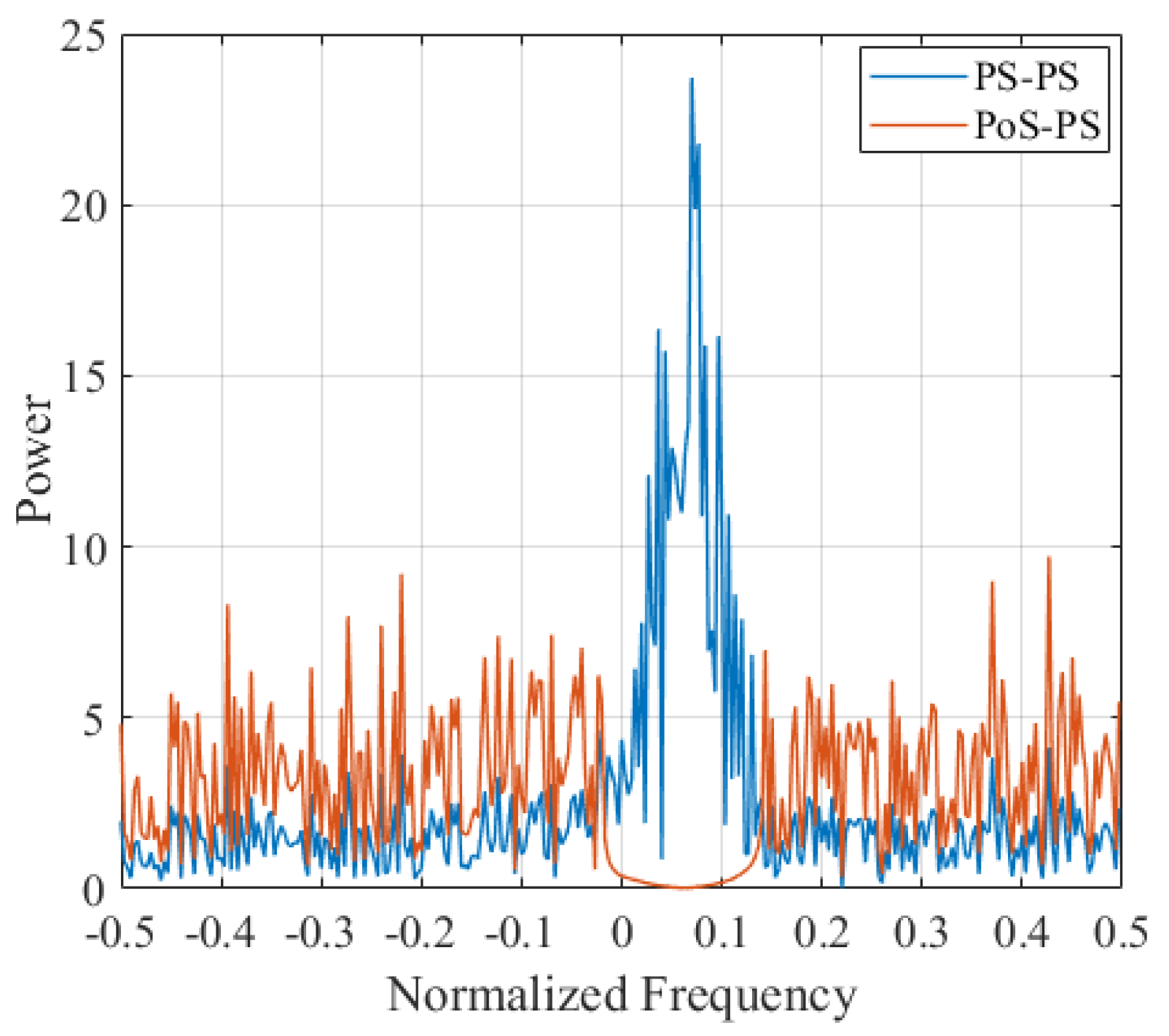Figure 2 illustrates the change in the normalized power spectrum of the sea clutter before and after applying the algorithm.

Due to the movement of the sea surface driven by wind, the radar echoes from the sea surface exhibit a frequency shift. As a result, the spectral peak position of the sea clutter power spectrum reflects the frequency shift induced by sea surface motion. As shown in Figure 2, after applying the proposed method, the spectral peak of the sea clutter power spectrum is significantly reduced. This is because the autocorrelation function effectively characterizes the complex signal form of sea clutter, and the suppression algorithm can adaptively match the autocorrelation characteristics of the actual sea clutter, filtering out a significant portion of the echoes from the moving sea surface, thereby reducing the intensity of the sea clutter. 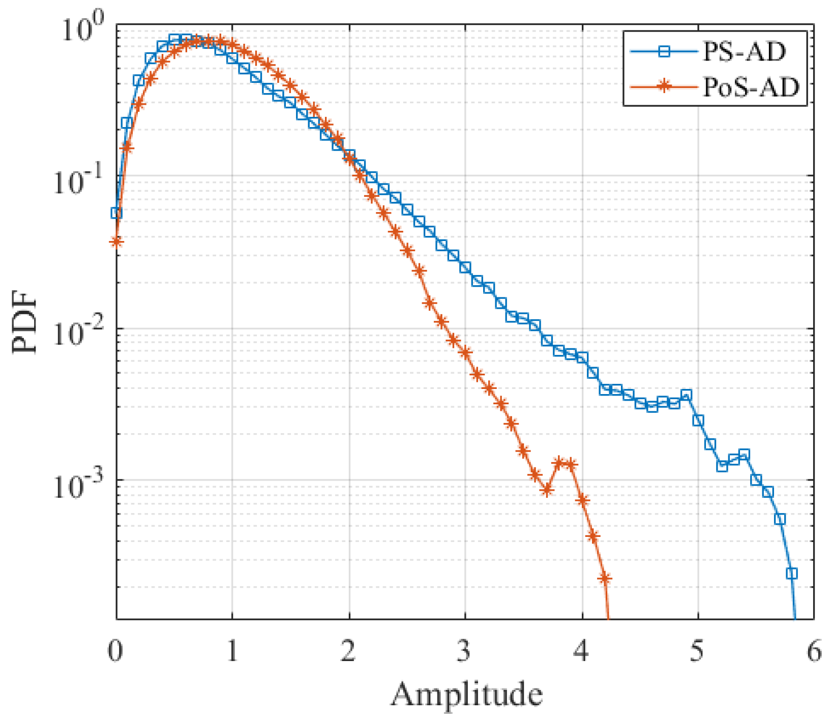Figure 3 displays the amplitude distribution of the sea clutter sample, as well as the amplitude distribution after applying the sea clutter suppression method proposed in this paper.

As shown in Figure 3, the tailing features in the sea clutter amplitude distribution are significantly reduced after applying the proposed method. This indicates that the sea clutter caused by the motion of the sea surface, especially the sharp peak echoes, has been effectively suppressed. Since these sharp peak echoes have a substantial impact on target detection performance, suppressing them can significantly enhance the target detection results. In the sea clutter suppression experiment presented in this paper, the number of eigenvalues was determined to be 52 using the Gerschgorin disk method. Given 200 range cells, 300 pulses, and 52 selected eigenvectors, the overall computational complexity of the proposed method is approximately $O(5.5\times {10}^7)$. This level of complexity is relatively low, indicating strong potential for real-time implementation. The simulation results presented later will further confirm this improvement.

5.2. Improvement of SCR by the Proposed Method

In this section, we consider a scenario where a target is present and analyze the impact of the proposed method on the SCR performance. To ensure the reliability of the experimental results, we continue to use real measured data for comparative analysis. Specifically, we selected sea clutter samples by extracting 300 consecutive pulses from range cells 2000 to 2200 in the data file “$20210106155330\_01\_$staring”. A moving target was added at the 100th range cell of the sea clutter sample, with the SCR set to 0 dB. The target was moving toward the radar at a speed of 3 m/s. The SCR is defined as the ratio of the target signal power to the sea clutter power, and is expressed as:

$$SCR\left(\mathrm{dB}\right)=10{log}_{10}({\displaystyle \frac{{\left|a\right|}^2·{\left|\right|p\left|\right|}^2}{N·P_{clutter}}})$$

(25)

Here, a denotes the amplitude of the target, p represents the steering vector of the target, $P_{clutter}$ indicates the average power of the sea clutter, N is the number of pulses, and dB denotes that the power values are expressed in decibels.

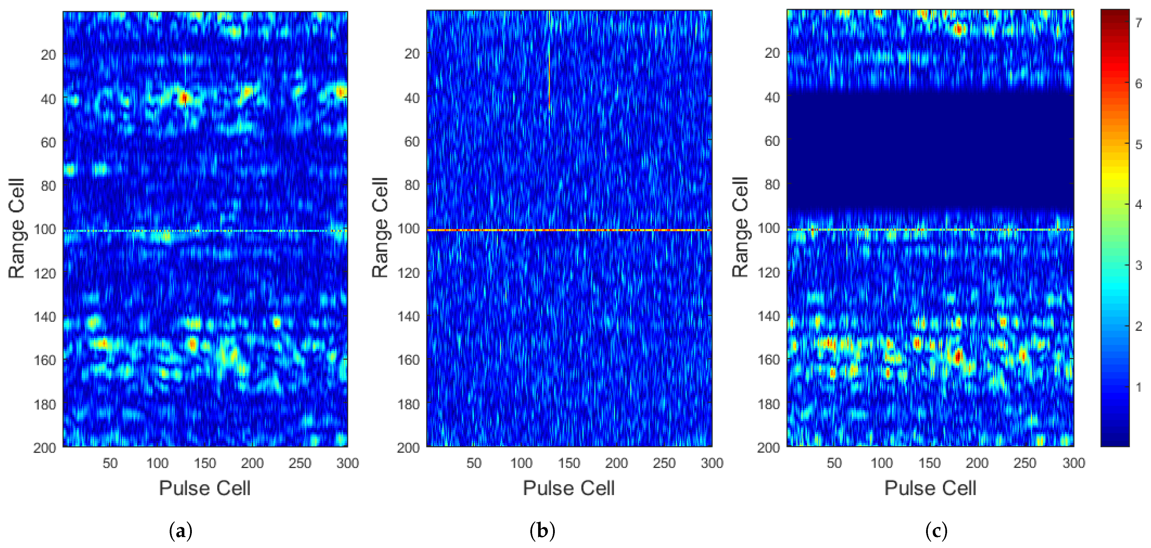
Figure 4a shows the unprocessed range-time image, while Figure 4b presents the result after applying the proposed method. For comparison, we also adopt the method from [21], where 50 range cells in front of the target are selected as reference samples to construct the clutter covariance matrix. To ensure consistency in comparison, the method also uses the Gerschgorin disk method to extract eigenvectors for sea clutter suppression. The corresponding result is shown in Figure 4c.

As observed in Figure 4, the original image shows that the target is completely submerged in the sea clutter and is difficult to identify by the naked eye. However, after applying the proposed suppression method, the sea clutter is significantly reduced and becomes more uniformly distributed, allowing the target to be clearly revealed. This improvement is due to the suppression algorithm’s ability to effectively filter out a large amount of clutter echoes originating from the moving sea surface, thereby enhancing the detectability of targets whose motion characteristics differ from those of the sea surface. In contrast, although the method from [21] performs well in suppressing sea clutter within the reference cells, it shows limited suppression capability in the vicinity of the target cell, making the target still difficult to distinguish. In addition, the computational complexity of the proposed method is approximately $O(5.5\times {10}^7)$, while that of the method in [21] is approximately $O(5.9\times {10}^7)$, and the complexity of the MTI method is about $O(3\times {10}^4)$. Since MTI uses a simple linear filtering operation and does not involve complex matrix computations, it has the lowest computational complexity. The proposed method avoids covariance matrix estimation and simultaneously reduces the computational load during target detection. Therefore, compared with [21], the computational complexity of the proposed method is significantly lower.

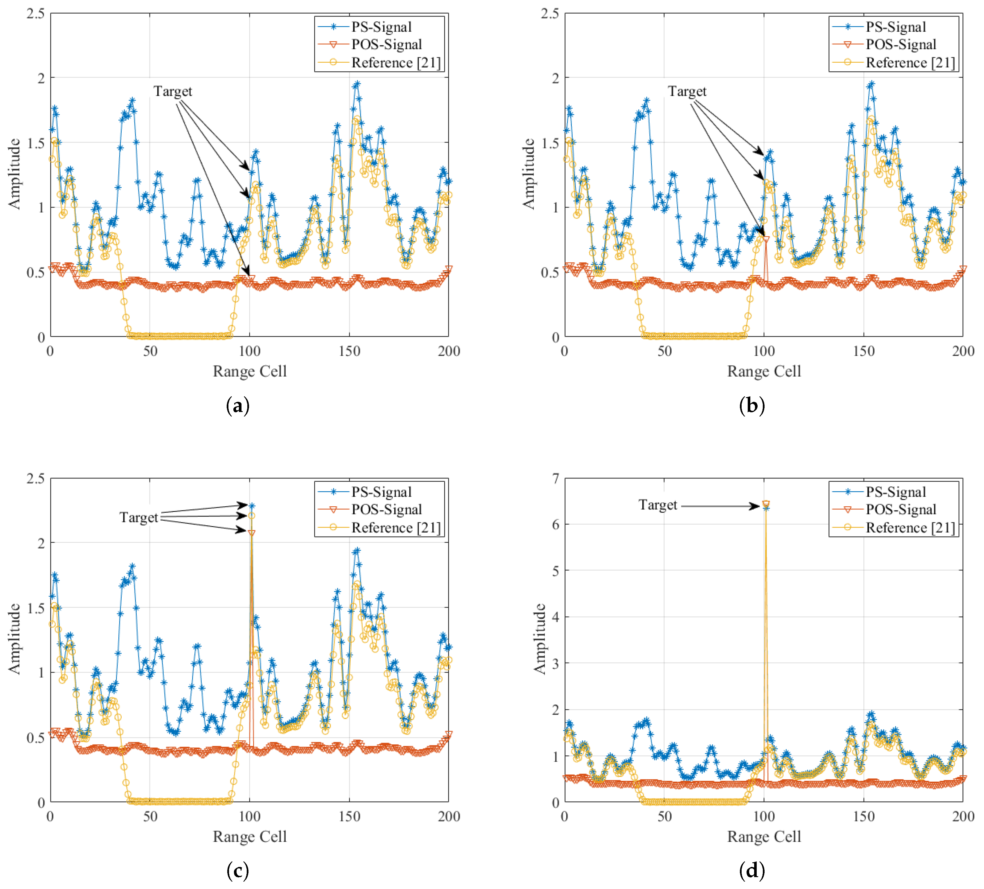
To validate the effectiveness of the proposed suppression method in enhancing the SCR, non-coherent integration was performed on 300 selected pulses. With the target velocity set to 3 m/s, the proposed method was compared with Reference [21] in terms of non-coherent integration performance after sea clutter suppression under SCR conditions of −10 dB, −5 dB, 0 dB, and 5 dB. The processing results are presented in Figure 5.

As shown in Figure 5, the unprocessed range-time images reveal that the target becomes clearly observable only when the SCR reaches 0 dB. At SCR = $-5$ dB, the target is almost completely obscured by sea clutter and becomes hardly discernible. After processing with the proposed method, however, the target maintains clear visibility along the range dimension even under low SCR conditions (SCR = $-5$ dB), demonstrating superior sea clutter suppression capability. In contrast, while Reference [21]’s method achieves effective clutter suppression in reference cells, its performance deteriorates significantly near the target cell, resulting in inadequate target-clutter separation.

5.3. Verification Using Simulated Data

This section presents an experiment based on simulated sea clutter data to verify the effectiveness of the proposed method in improving the Signal-to-Clutter Ratio (SCR). The sea clutter data were generated using the modeling approach proposed in [29], which is based on the SIRP (Spherically Invariant Random Process) model. In this model, the texture component governs the amplitude variation of the sea clutter, while the speckle component describes its temporal and spatial correlation characteristics. The amplitude distribution model used in [29] is the CG-IG distribution, and the temporal correlation function model is as follows:

$$f_{time}\left(m\right)=exp(-{\sigma }_{time}m+j{\omega }_{time}m)$$

(26)

Here, ${\sigma }_{time}$ is a parameter that determines the strength of temporal correlation; ${\omega }_{time}$ is a parameter that controls the periodicity of the correlation function and is related to the central Doppler shift of the clutter; and m represents the time lag index.

The spatial correlation function model used in [29] is as follows:

$$f_{space}\left(n\right)=exp(-{({\sigma }_{space}·n)}^2)$$

(27)

Here, ${\sigma }_{space}$ is a parameter that determines the strength of spatial correlation, and n represents the range lag index.

To obtain statistical characteristics representative of real-world scenarios, we adopted the parameter extraction method proposed in [29] and applied it to the data from range cells 2000 to 2200 in the file “$20210106155330\_01\_$staring”. The corresponding sea clutter statistical parameters are shown in

Table 2. Sea clutter statistical parameters of “$20210106155330\_01\_$staring”.

Characteristic	Parameter
Amplitude distribution	v = 1.378
a	b = 1.396
Temporal correlation	${\sigma }_{time}$ = 0.185
a	${\omega }_{time}$ = 0.418
Spatial correlation	${\sigma }_{space}$ = 0.264

.

Based on the statistical parameters extracted in Table 1, simulated sea clutter data were generated. To investigate the impact of individual parameters on the effectiveness of sea clutter suppression, each parameter was varied independently while keeping the remaining statistical parameters unchanged. The effectiveness of clutter suppression was quantitatively evaluated using the improvement in SCR, which is defined as:

$$TheimprovementinSCR={\displaystyle \frac{Post-suppressionSCR}{Pre-suppressionSCR}}$$

(28)

It is important to note that the SCR used in the above expression refers to the linear ratio of signal power to clutter power, rather than the decibel (dB) value.

In the simulation experiments, the target SCR was set to 5 dB. A total of 100 Monte Carlo trials were conducted, and the results were averaged for analysis. Figure 6 illustrates the impact of different statistical parameters on the SCR improvement capability. Specifically, Figure 6a shows the effect of the shape parameter v; Figure 6b shows the effect of the temporal correlation parameter ${\sigma }_{time}$; Figure 6c shows the effect of the temporal periodicity parameter ${\omega }_{time}$; and Figure 6d presents the influence of the spatial correlation parameter ${\sigma }_{space}$.

According to the SIRP theory, in the CG-IG distribution, the shape parameter v in the texture component reflects the heavy-tailed characteristics of sea clutter amplitudes. An increase in v indicates a higher occurrence of sea spikes within the clutter. As shown in Figure 6a, the SCR improvement increases with the shape parameter v, which demonstrates that the proposed algorithm is effective in suppressing sea spikes in the clutter. According to Equation (25), as the temporal correlation parameter ${\sigma }_{time}$ increases, the temporal correlation weakens. Since the proposed method designs an orthogonal projection operator based on the temporal correlation function, Figure 6b shows that the sea clutter suppression performance improves with stronger temporal correlation. In addition, the temporal periodicity parameter ${\omega }_{time}$ affects the frequency range of the sea clutter. As shown in Figure 6c, the proposed method exhibits adaptability in suppressing sea clutter across different frequency ranges. According to Equation (26), as the spatial correlation parameter ${\sigma }_{space}$ increases, the spatial correlation decreases. Figure 6d shows that with stronger spatial correlation, the frequency band in which clutter is suppressed becomes narrower. This is because spatial correlation primarily reflects the power distribution characteristics of sea clutter along the range dimension, while the texture component describes the local variation of clutter power. When sea clutter exhibits strong spatial correlation in the range dimension, its local power variation becomes more stable, resulting in reduced fluctuation in the texture component. As previously derived, the magnitude of the texture component directly affects both the number of eigenvalues and eigenvectors representing sea clutter. When the texture component increases, the dimensionality of the clutter subspace decreases accordingly, thereby reducing the range of clutter subspace that can be effectively suppressed in the frequency domain by the proposed method. This ultimately leads to a narrower frequency band over which the clutter can be suppressed.

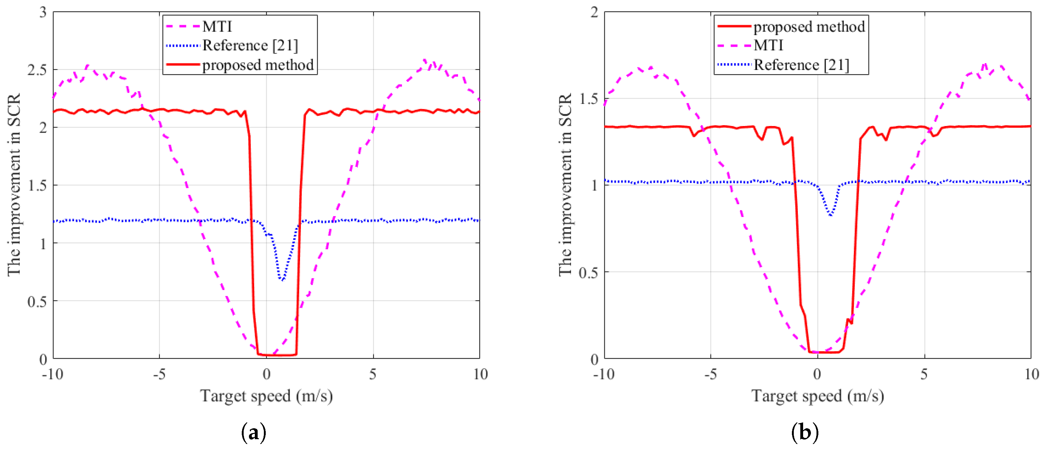
5.4. Verification Using Real Sea Clutter Data

To further validate the effectiveness of the proposed method under real sea clutter conditions, a comparative study was conducted using measured data. The performance of the proposed method, the method in [21], and the conventional Moving Target Indication (MTI) method was evaluated in terms of SCR improvement. The sea clutter suppression performance was compared under different sea states to further confirm the reliability of the simulation results. The measured data used in this experiment were obtained under sea state levels 3–4 and level 2, both from the file “$20210106155330\_01\_$staring” A pure sea clutter region was selected from range cells 1900 to 2100, and 300 consecutive pulses were extracted for processing. To improve statistical reliability, 100 Monte Carlo simulations were performed, and the results were averaged. The final experimental results are presented in Figure 7.

As shown by the variation in SCR improvement capability in Figure 6, the proposed method outperforms the method in [21] in terms of sea clutter suppression. This is primarily attributed to the fact that the proposed algorithm fully considers the overall frequency characteristics of sea clutter during its design, thereby offering stronger adaptability. In contrast, the method in [21] mainly relies on suppressing clutter within the reference cells, with limited suppression capability near the target cell. As a result, its overall effectiveness in SCR enhancement is less significant. The MTI method essentially functions as a high-pass filter, effectively suppressing stationary clutter near zero Doppler frequency. When the target has a high velocity, its Doppler shift moves away from the zero-frequency band, making the signal more distinguishable. In such cases, MTI demonstrates better SCR enhancement performance. Although traditional MTI methods have some clutter suppression capability, they lack the ability to adaptively match the spectral characteristics of sea clutter. As a result, when the target is near zero Doppler frequency, MTI may suppress the target signal along with the clutter, thereby degrading detection performance. A further comparison between Figure 8a,b reveals that the proposed method demonstrates more pronounced suppression performance under high sea state conditions. This is due to the stronger spikiness and higher temporal correlation of sea clutter in rougher sea states. These experimental results are consistent with the conclusions previously drawn from the simulated sea clutter data.

In addition, the classical CA-CFAR (Cell-Averaging Constant False Alarm Rate) method [41] was employed to evaluate the effectiveness of the proposed method in improving target detection performance. Through Monte Carlo simulations, the detection probability (PD) of CA-CFAR under various SCR levels was studied for a target with a radial velocity of −3 m/s. The data used in this experiment were drawn from two sources: (1) a sea clutter region corresponding to range cells 2000 to 2200 in the SDRDSP dataset file “$20210106155330\_01\_$staring” from which 300 consecutive pulses were randomly selected; and (2) real radar measurements collected by IPIX in 1998, specifically, the file “$19980223\_192144\_$antstep” from which another 300 consecutive pulses were randomly extracted [42]. The number of non-coherent integrations was set to 300, and 1000 Monte Carlo trials were performed to ensure statistical reliability. Under a fixed false alarm probability of 0.001, the relationship between SCR and detection probability was obtained, as shown in Figure 8.

The results in the figure show that the proposed method effectively suppresses sea clutter by constructing a clutter feature subspace and applying orthogonal projection. However, under low SCR conditions, the constructed subspace may still contain frequency components outside the clutter, leading to partial suppression of the target signal and reduced detection performance. In contrast, the MTI method, which uses a high-pass filter to directly suppress near-zero Doppler clutter, retains weak target signals with Doppler frequencies away from zero more effectively, giving it an advantage in extremely low SCR scenarios. Nevertheless, across a range of SCR values, the proposed method consistently outperforms both the MTI method and the approach in Reference [21] in terms of detection probability. This performance gain is primarily attributed to the proposed suppression strategy’s ability to effectively eliminate strong sea clutter echoes, thereby enhancing the relative prominence of target signals and significantly improving the detection performance for small targets over the sea surface.

6. Conclusions

This paper proposes a sea clutter suppression method based on autocorrelation features to address the problem of detecting small maneuvering targets in sea clutter environments. The method constructs speckle components using the autocorrelation characteristics of the observed data and extracts the sea clutter feature subspace. By applying orthogonal projection, clutter suppression is achieved without relying on covariance matrix estimation from adjacent reference cells, which significantly enhances the robustness and adaptability of the algorithm. To validate the effectiveness of the proposed method, both simulated and real measured data were used for comparative analysis against two traditional approaches. Experimental results show that, compared with the orthogonal projection method relying on reference cell covariance estimation, the proposed method performs better in terms of target energy enhancement, SCR improvement, and detection probability. In comparison with the MTI method, the proposed approach is more capable of adapting to Doppler shifts in sea clutter and demonstrates stronger overall clutter suppression. Moreover, the method features a clear structure and moderate computational complexity, requires no training data or extensive prior knowledge, and exhibits strong potential for real-time implementation. In conclusion, the proposed method provides an efficient, robust, and practical solution for detecting small maneuvering targets in complex sea clutter environments.