
Analysis of Offshore Pile–Soil Interaction Using Artificial Neural Network


Abstract
1. Introduction
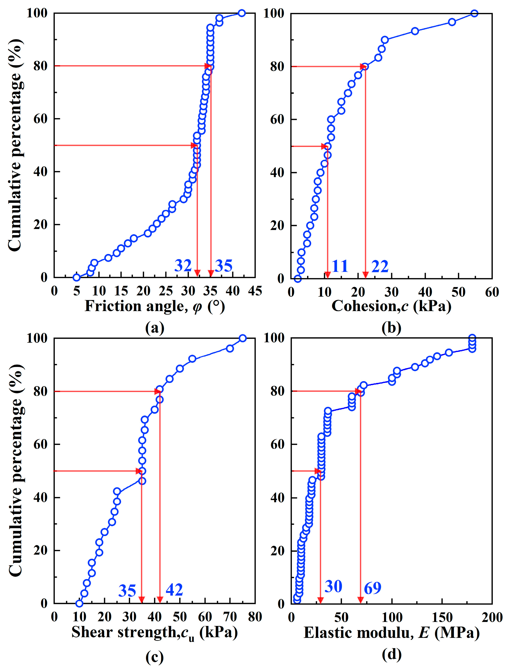
2. Database
3. Neural Network Modeling of Pile–Soil Interaction
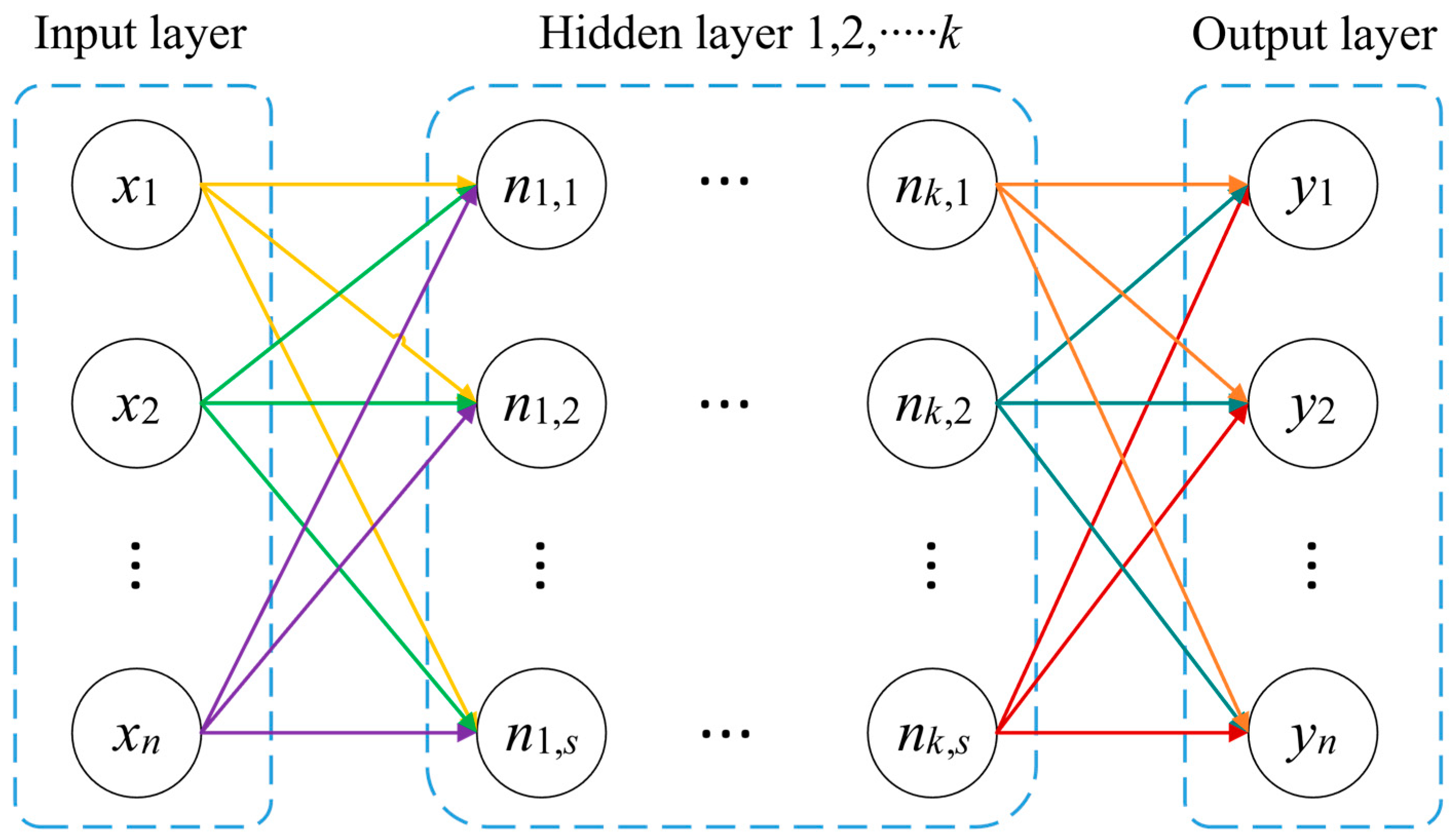
3.1. Artificial Neural Networks
3.2. Architecture Design & Workflow
3.2.1. Data Preprocessing
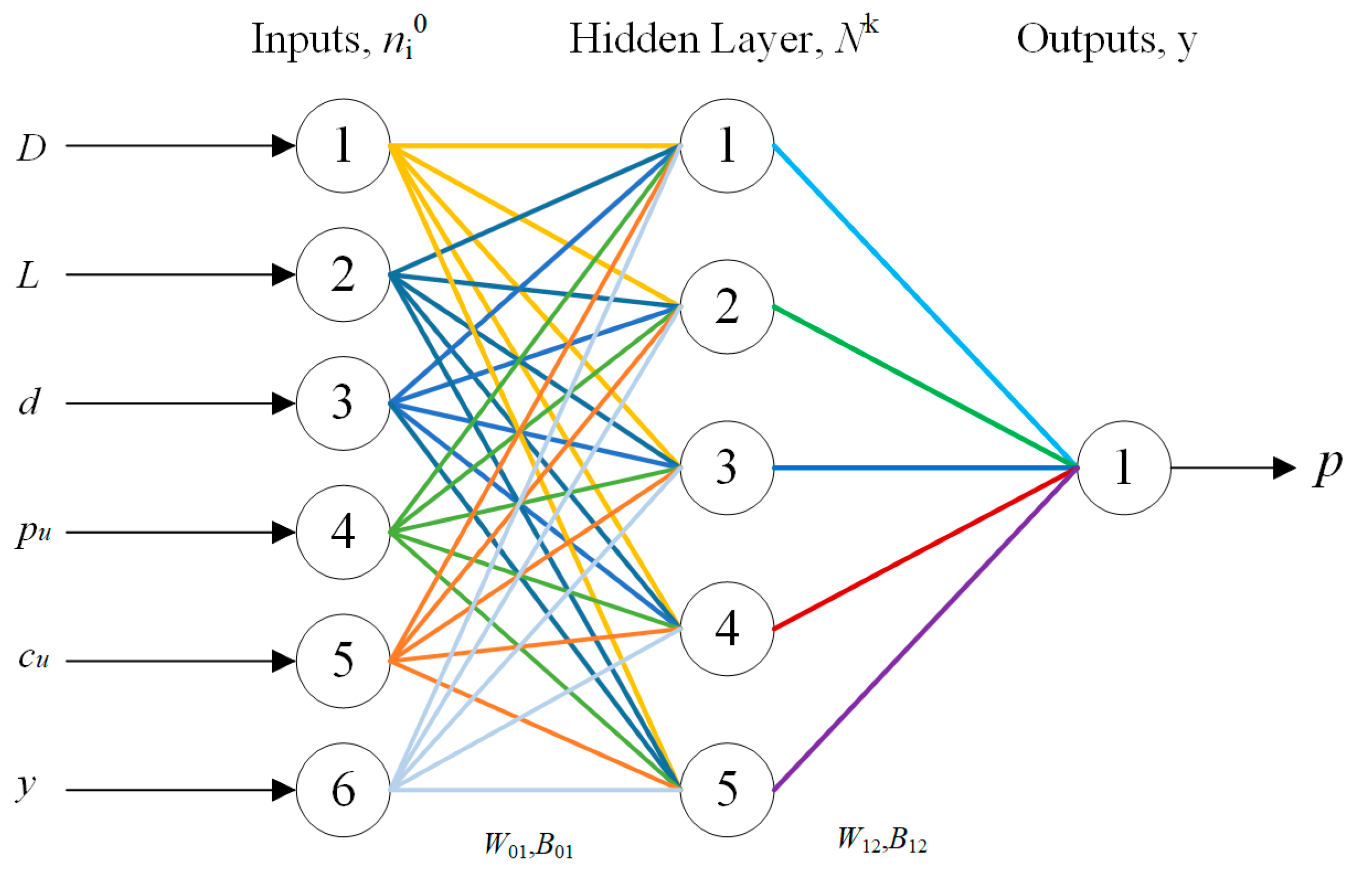
3.2.2. Topology Structure
3.2.3. Propagation Mechanism & Training Algorithm
3.2.4. Learning Rate & Iterations
3.2.5. Validation and Regularization
4. Results
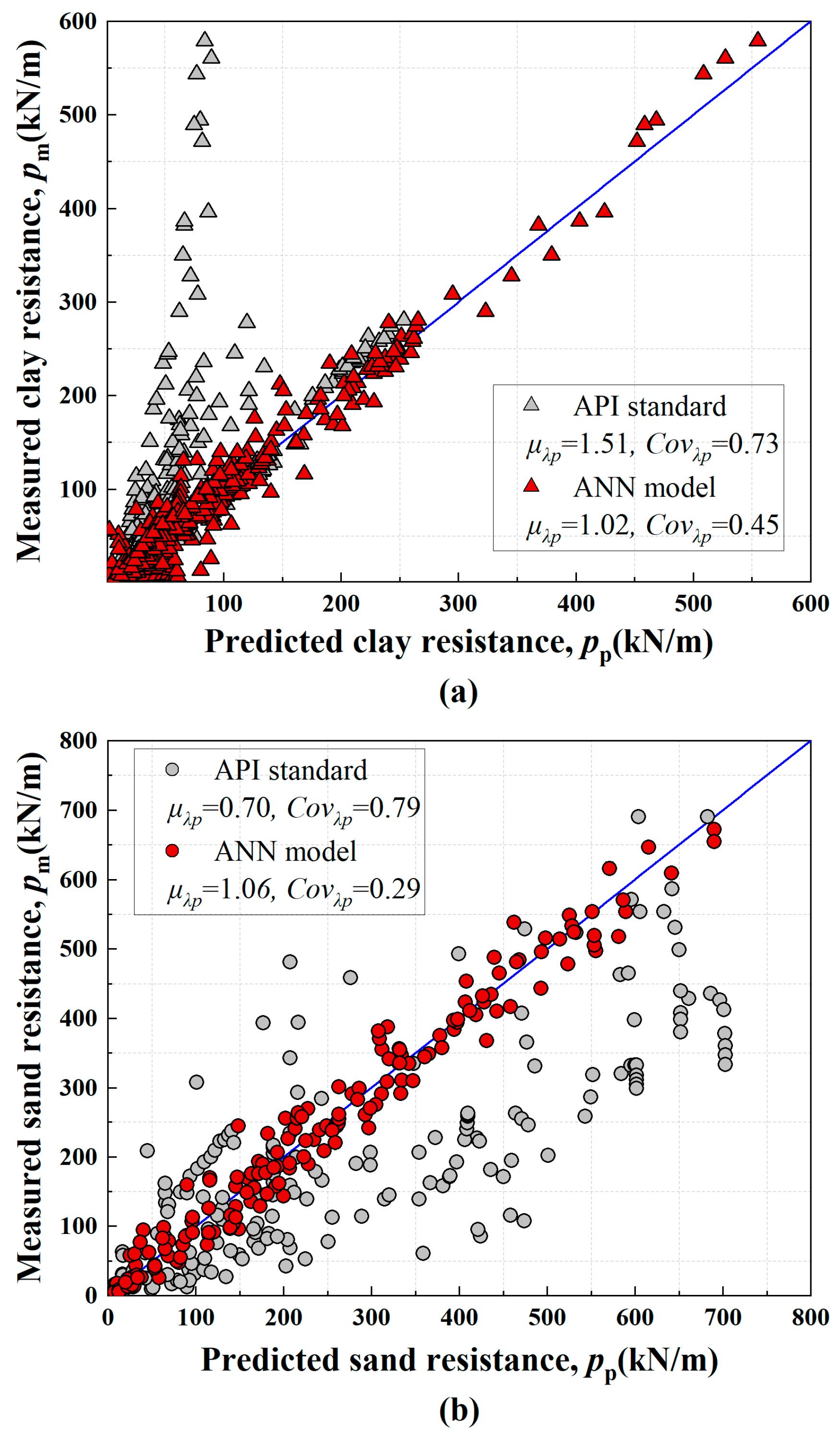
4.1. Predictions of p-y Curves
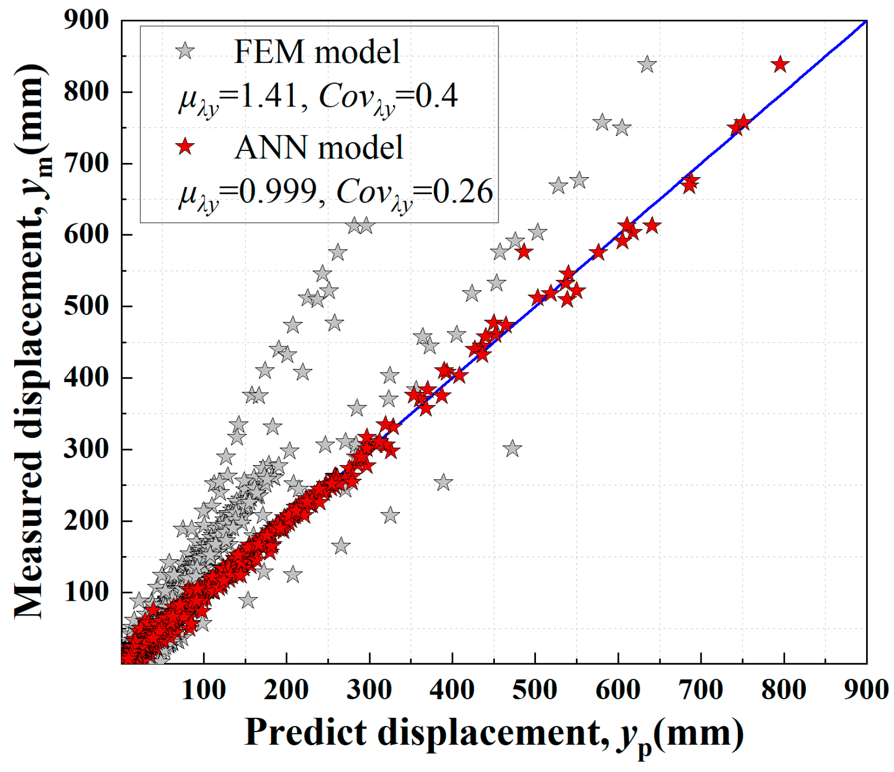
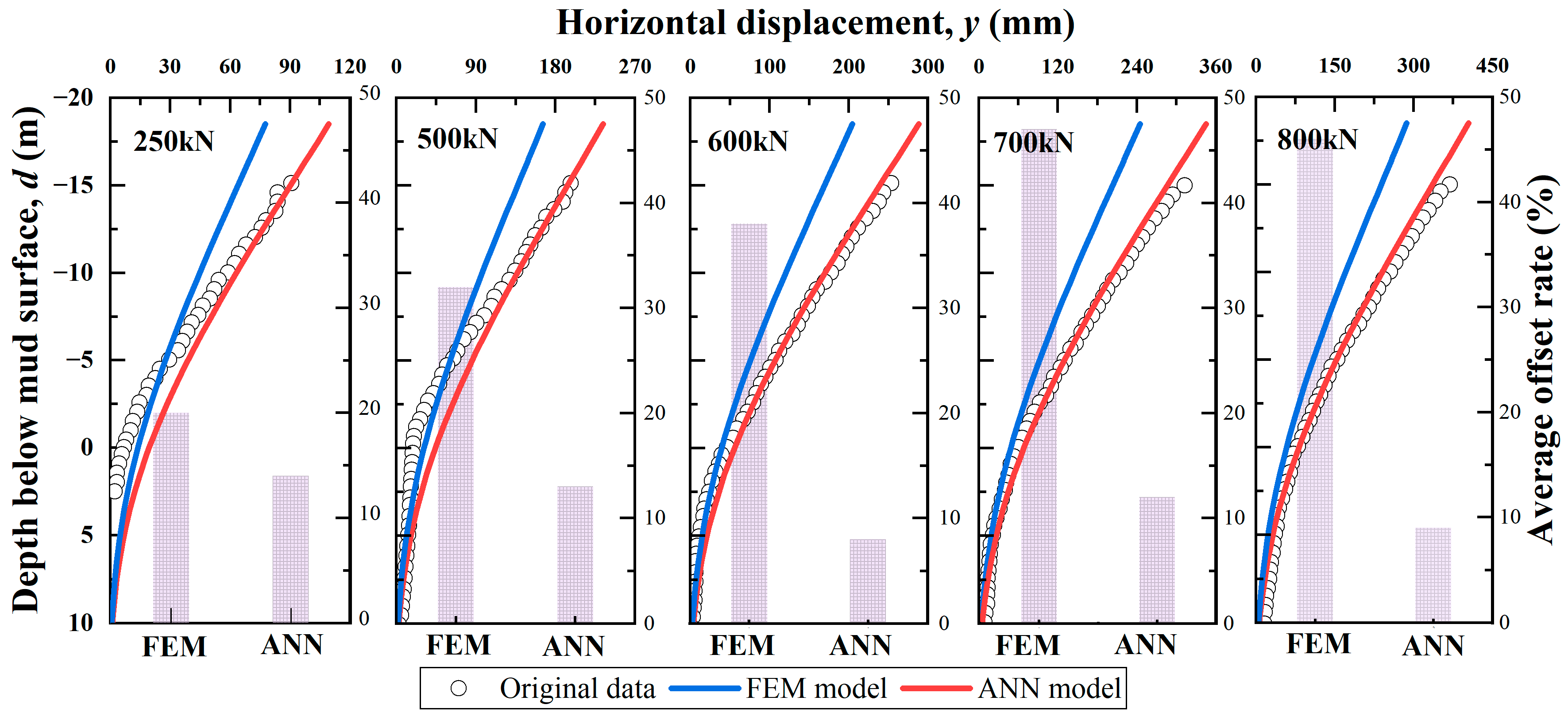
4.2. Pile Horizontal Displacement Prediction
5. Discussion
5.1. Model Performance
5.2. Parameter Sensitivity
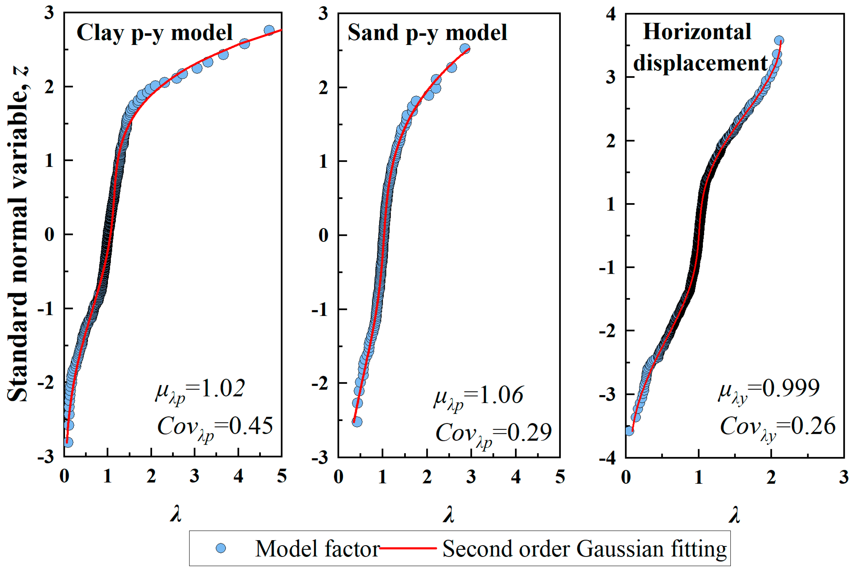
5.3. Probability Distribution
5.4. Case Application
6. Conclusions
Author Contributions
Funding
Data Availability Statement
Conflicts of Interest
Abbreviations
| ak | Activation of the k-th hidden neuron |
| A-D | Anderson–Darling |
| ANN | Artificial neural network |
| API | American Petroleum Institute |
| B01 | 5 × 1 bias vector |
| B12 | Hidden-to-output layer bias vector |
| bk,t | Bias vector of the layer |
| c | Cohesion |
| cu | Shear strength |
| COVλ | Coefficient of variation |
| d | Depth |
| D | Outer diameter |
| e | Residual vector |
| E | Elastic modulus |
| f(x) | Activation functions (logistic) |
| FEM | Finite element method |
| F | Horizontal force applied at the pile head |
| i | Total number of samples |
| Identity matrix | |
| Jacobian matrix of partial derivatives | |
| The transpose of the Jacobian matrix | |
| K-S | Kolmogorov–Smirnov |
| l | Distance from the test point to the pile top |
| L | Pile length |
| Regularized loss function | |
| LM | Levenberg–Marquardt |
| m | Number of hidden nodes |
| MSE | Mean squared error |
| n | Input dimension |
| The p-th input to the k-th neuron | |
| pu | Ultimate resistance |
| Pm | Measured soil resistance |
| Pp | Predicted soil resistance |
| Nmax | Maximum iteration threshold |
| Input vector | |
| Output vector of the first hidden layer | |
| p | Mobilized soil resistance |
| R2 | Coefficient of determination |
| SVM | Support vector machines |
| t | Wall thickness |
| wk,p,t | Weight matrix of the layer |
| W01 | 5 × 6 weight matrix |
| W12 | Hidden-to-output layer weight matrix |
| x | Raw data |
| Normalized value | |
| Maximum value | |
| Minimum value | |
| y | Lateral soil displacement |
| ym | Measured displacement |
| yp | Predicted displacement |
| Normalized bound of measured input parameters | |
| Normalized bound of measured input parameters | |
| Predicted value | |
| Actual value | |
| zk | Pre-activation of the k-th hidden neuron |
| Change in validation loss | |
| Weight update vector | |
| α | Hyperparameter optimized via cross-validation. |
| β | Hyperparameter optimized via cross-validation |
| φ | Internal friction angle |
| μ | Damping factor |
| η | Learning rate |
| γ | Soil’s unit weight |
| λ | Model factorMean value |
| μλ | |
| Squared error | |
| Mean squared error | |
| Regularization penalty term |
References
- IEA. Offshore Wind Outlook 2019; IEA: Paris, France, 2019. [Google Scholar]
- Hjelmeland, M.; Nøland, J.K. Correlation Challenges for North Sea Offshore Wind Power: A Norwegian Case Study. Sci. Rep. 2023, 13, 18670. [Google Scholar] [CrossRef] [PubMed]
- Santhakumar, S.; Meerman, H.; Faaij, A.; Martinez Gordon, R.; Florentina Gusatu, L. The Future Role of Offshore Renewable Energy Technologies in the North Sea Energy System. Energy Convers. Manag. 2024, 315, 118775. [Google Scholar] [CrossRef]
- Ponder, A.N.; Avdic, D.B. Offshore Wind and Power-to-Hydrogen in the Baltic Sea Region; BOWE2H Strategic Roadmap; IKEM: Berlin, Germany, 2024. [Google Scholar]
- Ren, L.; Wang, Y.; Zhang, W.; Yang, H.; Wang, H.; Wei, J.; Mateos, L.M.F. Characterizing Wind Fields at Multiple Temporal Scales: A Case Study of the Adjacent Sea Area of Guangdong–Hong Kong–Macao Greater Bay Area. Energy Rep. 2022, 8, 212–223. [Google Scholar] [CrossRef]
- Sun, Y. Experimental and Numerical Studies on a Laterally Loaded Monopile Foundation of Offshore Wind Turbine. Ph.D. Thesis, Zhejiang University, Hangzhou, China, 2016. [Google Scholar]
- Zhang, J.; Wang, H. Development of Offshore Wind Power and Foundation Technology for Offshore Wind Turbines in China. Ocean Eng. 2022, 266, 113256. [Google Scholar] [CrossRef]
- Buljac, A.; Kozmar, H.; Yang, W.; Kareem, A. Concurrent Wind, Wave and Current Loads on a Monopile-Supported Offshore Wind Turbine. Eng. Struct. 2022, 255, 113950. [Google Scholar] [CrossRef]
- Yang, Y.F.; Zheng, Y.Q.; Ge, H.; Wang, C.Z. Nonlinear Interactions between Solitary Waves and Structures in a Steady Current. Ocean Eng. 2023, 274, 113920. [Google Scholar] [CrossRef]
- Yu, Y.; Chen, X.; Guo, Z.; Zhang, J.; Lü, Q. Robust Design of Monopiles for Offshore Wind Turbines Considering Uncertainties in Dynamic Loads and Soil Parameters. Ocean Eng. 2022, 266, 112822. [Google Scholar] [CrossRef]
- Qi, W.; Gao, F. Equilibrium Scour Depth at Offshore Monopile Foundation in Combined Waves and Current. Sci. China Technol. Sci. 2014, 57, 1030–1039. [Google Scholar] [CrossRef]
- Gupta, B.K. Soil-Structure Interaction Analysis of Monopile Foundations Supporting Offshore Wind Turbines. Ph.D. Thesis, University of Waterloo, Waterloo, ON, Canada, 2018. [Google Scholar]
- Poulos, H.G. Pile Behaviour—Theory and Application. Géotechnique 1989, 39, 365–415. [Google Scholar] [CrossRef]
- Hansen, N.M. Interaction Between Seabed Soil and Offshore Wind Turbine Foundations; DCAMM Special Report; DTU Mechanical Engineering: Lyngby, Denmark, 2012; ISBN 9788790416805. [Google Scholar]
- Zhu, B.; Wen, K.; Li, T.; Wang, L.; Kong, D. Experimental Study on Lateral Pile–Soil Interaction of Offshore Tetrapod Piled Jacket Foundations in Sand. Can. Geotech. J. 2019, 56, 1680–1689. [Google Scholar] [CrossRef]
- Sheil, B.B.; McCabe, B.A. An Analytical Approach for the Prediction of Single Pile and Pile Group Behaviour in Clay. Comput. Geotech. 2016, 75, 145–158. [Google Scholar] [CrossRef]
- Shi, S.; Zhai, E.; Xu, C.; Iqbal, K.; Sun, Y.; Wang, S. Influence of Pile-Soil Interaction on Dynamic Properties and Response of Offshore Wind Turbine with Monopile Foundation in Sand Site. Appl. Ocean Res. 2022, 126, 103279. [Google Scholar] [CrossRef]
- Tang, H.; Yue, M.; Yan, Y.; Li, Z.; Li, C.; Niu, K. Influence of Soil–Structure Interaction Models on the Dynamic Responses of An Offshore Wind Turbine Under Environmental Loads. China Ocean Eng. 2023, 37, 218–231. [Google Scholar] [CrossRef]
- Chow, Y.K.; Kencana, E.Y.; Leung, C.F.; Purwana, O.A. Spudcan-Pile Interaction in Thick Soft Clay and Soft Clay Overlying Sand: A Simplified Numerical Solution. Appl. Ocean Res. 2021, 112, 102684. [Google Scholar] [CrossRef]
- Lin, Z.; Jiang, Y.; Xiong, Y.; Xu, C.; Guo, Y.; Wang, C.; Fang, T. Analytical Solution for Displacement-Dependent Active Earth Pressure Considering the Stiffness of Cantilever Retaining Structure in Cohesionless Soil. Comput. Geotech. 2024, 170, 106258. [Google Scholar] [CrossRef]
- Randolph, M.F. The Response of Flexible Piles to Lateral Loading. Géotechnique 1981, 31, 247–259. [Google Scholar] [CrossRef]
- Heidari, M.; Hesham El Naggar, M. Analytical Approach for Seismic Performance of Extended Pile-Shafts. J. Bridge Eng. 2018, 23, 04018069. [Google Scholar] [CrossRef]
- American Petroleum Institute. Planning, Designing, and Constructing Fixed Offshore Platforms: Working Stress Design; API: Washington, DC, USA, 2020. [Google Scholar]
- DET NORSKE VERITAS DNVGL-ST-N001; Marine Operations and Marine Warranty; DNV GL: Oslo, Norway, 2016.
- MOT China Communications Press. JTS 167-2018: Code for Design of Pile Foundations in Port and Waterway Engineering; China Communications Press: Beijing, China, 2022. [Google Scholar]
- Liu, P.; Jiang, C. A Modified P-y Curve Model for Offshore Piles near Sandy Slopes Considering the Soil-Pile-Slope Deformation Mechanism. Mar. Struct. 2024, 98, 103675. [Google Scholar] [CrossRef]
- Stevens, J.B.; Audibert, J.M.E. Re-Examination Of P-Y Curve Formulations. In Proceedings of the Offshore Technology Conference, Houston, TX, USA, 30 April–3 May 1979. [Google Scholar]
- Wang, H.; Wang, L.Z.; Hong, Y.; He, B.; Zhu, R.H. Quantifying the Influence of Pile Diameter on the Load Transfer Curves of Laterally Loaded Monopile in Sand. Appl. Ocean Res. 2020, 101, 102196. [Google Scholar] [CrossRef]
- White, D.J.; Doherty, J.P.; Guevara, M.; Watson, P.G. A Cyclic P-y Model for the Whole-Life Response of Piles in Soft Clay. Comput. Geotech. 2022, 141, 104519. [Google Scholar] [CrossRef]
- Lin, P.; Zhong, X.; Guo, C.; Yang, F.; Wang, F. Statistical Evaluation of Jacking-Installation Resistance Models for Suction Foundation of Offshore Wind Turbines in Sands. Ocean Eng. 2023, 279, 114605. [Google Scholar] [CrossRef]
- Yeter, B.; Garbatov, Y.; Guedes Soares, C. Uncertainty Analysis of Soil-Pile Interactions of Monopile Offshore Wind Turbine Support Structures. Appl. Ocean Res. 2019, 82, 74–88. [Google Scholar] [CrossRef]
- Byrne, B.W.; Houlsby, G.T.; Burd, H.J.; Gavin, K.G.; Igoe, D.J.P.; Jardine, R.J.; Martin, C.M.; McAdam, R.A.; Potts, D.M.; Taborda, D.M.G.; et al. PISA Design Model for Monopiles for Offshore Wind Turbines: Application to a Stiff Glacial Clay Till. Géotechnique 2020, 70, 1030–1047. [Google Scholar] [CrossRef]
- Haiderali, A.; Madabhushi, G. Three-Dimensional Finite Element Modelling of Monopiles for Offshore Wind Turbines. In Proceedings of the Advances in Civil, Environmental, and Materials Research, Seoul, Republic of Korea, 26–29 August 2012. [Google Scholar]
- McAdam, R.A.; Byrne, B.W.; Houlsby, G.T.; Beuckelaers, W.J.A.P.; Burd, H.J.; Gavin, K.G.; Igoe, D.J.P.; Jardine, R.J.; Martin, C.M.; Muir Wood, A.; et al. Monotonic Laterally Loaded Pile Testing in a Dense Marine Sand at Dunkirk. Géotechnique 2020, 70, 986–998. [Google Scholar] [CrossRef]
- Xiao-ling, Z.; Rui, Z.; Yan, H. Study on P-y Curve of Large Diameter Pile under Long-Term Cyclic Loading. Appl. Ocean Res. 2023, 140, 103736. [Google Scholar] [CrossRef]
- Sheil, B.; Finnegan, W. Numerical Simulations of Wave–Structure–Soil Interaction of Offshore Monopiles. Int. J. Geomech. 2017, 17, 04016024. [Google Scholar] [CrossRef]
- Brinkgreve, R.B.; Bürg, M.; Andreykiv, A.; Lim, L. Beyond the Finite Element Method in Geotechnical Analysis; Bundesanstalt für Wasserbau: Karlsruhe, Germany, 2015; Volume 98, pp. 91–102. [Google Scholar]
- Lin, P.; Ding, M.; Liu, H.; Liu, Y.; Wang, K. Statistical Accuracy of Finite Element Method in Predicting Horizontal Displacement of Monopiles for Offshore Wind Turbines. Mar. Struct. 2024, 97, 103641. [Google Scholar] [CrossRef]
- Murphy, G.; Igoe, D.; Doherty, P.; Gavin, K. 3D FEM Approach for Laterally Loaded Monopile Design. Comput. Geotech. 2018, 100, 76–83. [Google Scholar] [CrossRef]
- Wang, S.; Han, B.; Jiang, J.; Telyatnikova, N. Machine Learning and FEM-Driven Analysis and Optimization of Deep Foundation Pits in Coastal Area: A Case Study in Fuzhou Soft Ground. Undergr. Space 2025, 22, 55–76. [Google Scholar] [CrossRef]
- Baghbani, A.; Choudhury, T.; Costa, S.; Reiner, J. Application of Artificial Intelligence in Geotechnical Engineering: A State-of-the-Art Review. Earth-Sci. Rev. 2022, 228, 103991. [Google Scholar] [CrossRef]
- Lin, P.; Zhao, C.; Zhang, W.; Xue, Y. Machine Learning Methods and Applications in Geotechnical Engineering; China Architecture & Building Press: Beijing, China, 2023. [Google Scholar]
- Vahab, M.; Shahbodagh, B.; Haghighat, E.; Khalili, N. Application of Physics-Informed Neural Networks for Forward and Inverse Analysis of Pile–Soil Interaction. Int. J. Solids Struct. 2023, 277–278, 112319. [Google Scholar] [CrossRef]
- Zhang, W.; Li, H.; Li, Y.; Liu, H.; Chen, Y.; Ding, X. Application of Deep Learning Algorithms in Geotechnical Engineering: A Short Critical Review. Artif. Intell. Rev. 2021, 54, 5633–5673. [Google Scholar] [CrossRef]
- Cui, C.; Zhang, S.; Chapman, D.; Meng, K. Dynamic Impedance of a Floating Pile Embedded in Poro-Visco-Elastic Soils Subjected to Vertical Harmonic Loads. Geomech. Eng. 2018, 15, 793–803. [Google Scholar] [CrossRef]
- Dong, Y.; Cui, L.; Zhang, X. Multiple-GPU Parallelization of Three-dimensional Material Point Method Based on Single-root Complex. Int. J. Numer. Methods Eng. 2022, 123, 1481–1504. [Google Scholar] [CrossRef]
- Cui, C.; Zhang, S.; Yang, G.; Li, X. Vertical Vibration of a Floating Pile in a Saturated Viscoelastic Soil Layer Overlaying Bedrock. J. Cent. South Univ. 2016, 23, 220–232. [Google Scholar] [CrossRef]
- Zhang, Y.; Zhong, W.; Li, Y.; Wen, L.; Sun, X. ResGRU: A Deep Learning Approach for Settlement Prediction in CFRD Based on the Spatiotemporal Feature Fusion Method. Comput. Geotech. 2024, 173, 106518. [Google Scholar] [CrossRef]
- Wang, W.; Yan, J.; Liu, J.P. Study on p-y Models for Large-Diameter Pile Foundation Based on In-Situ Tests of Offshore Wind Power. Chin. J. Geotech. Eng. 2021, 43, 1131–1138. [Google Scholar] [CrossRef]
- Hu, Z.; Zhai, E.; Luo, L.; Yang, X. Study of P-y Curves of Large-Monopiles for Offshore Wind Power in Sand. Acta Energiae Solaris Sin. 2019, 40, 3571–3577. [Google Scholar]
- Wu, R.; Ye, J.; Luo, G.; Shen, X.; Zhang, Q. Experimental Study on the Bearing Characteristics of Steel Pipe Pile in Radial Sandbar of Jiangsu Province. Ocean Eng. 2021, 39, 121–132. [Google Scholar] [CrossRef]
- Luo, L.; Wang, Y.; Zhai, E.; Hu, Z.; Yang, X.; Li, Q. Study on P-y Curves of Monopile in Layered Soil Based on Field Test. Acta Energiae Solaris Sin. 2019, 40, 3258–3264. [Google Scholar]
- Kim, Y.; Jeong, S.; Won, J. Effect of Lateral Rigidity of Offshore Piles Using Proposed P-y Curves in Marine Clay. Mar. Georesources Geotechnol. 2009, 27, 53–77. [Google Scholar] [CrossRef]
- Zhang, Y. Study on Horizontal Load Test of Large-Diameter Steel Pipe Piles for Offshore Wind Power. Energy Environ. 2022, 175, 18–20. [Google Scholar] [CrossRef]
- Gong, W.; Huo, S.; Yang, C.; Huang, X.; Guo, C. Experimental Study on Horizontal Bearing Capacity of Large Diameter Steel Pipe Pile for Offshore Wind Farm. J. Hydraul. Eng. 2015, 46, 34–39. [Google Scholar] [CrossRef]
- Bao, J.; Su, J.; Wu, F. Field Horizontal Loading Test and P-y Curve Applicability of Large-Diameter Single Pile Foundation in Deep Soft Clay Groundsill. J. Hohai Univ. (Nat. Sci.) 2023, 51, 127–134. [Google Scholar] [CrossRef]
- Liu, J.; Zhang, F.; Dai, G. Research on P-y Curve of Pile Foundation in Clay Based on Cpt Data. Acta Energiae Solaris Sin. 2023, 44, 172–180. [Google Scholar] [CrossRef]
- Zhu, B.; Zhu, Z.; Li, T.; Liu, J.; Liu, Y. Field Tests of Offshore Driven Piles Subjected to Lateral Monotonic and Cyclic Loads in Soft Clay. J. Waterw. Port. Coast. Ocean Eng. 2017, 143, 05017003. [Google Scholar] [CrossRef]
- Cai, W.; Ye, J. Experimental Investigation of Large Diameter Pipe Piles Under Vertical and Lateral Load in Ocean Engineering. Shanghai Land Resour. 2011, 32, 81–86. [Google Scholar] [CrossRef]
- Zhu, Z.; Gong, W.; DAI, G. Field Test Research of Horizontal Bearing Capacity of Large Diameter Steel Pipe Pile. Build. Sci. 2010, 26, 32–36. [Google Scholar] [CrossRef]
- Wang, Q.; Wang, S.; Wu, F. Research on Horizontal Load Testing of Large-Diameter Steel Pipe Piles. Ocean Dev. Manag. 2018, 35, 9–13. [Google Scholar] [CrossRef]
- Bi, M.; Liu, D.; Wang, H. Calculation Method Study for the Horizontal Bearing Capacity of Offshore Wind Turbine Steel-Pile. South. Energy Constr. 2018, 5, 77–82. [Google Scholar] [CrossRef]
- Lao, W.; Zhou, L.; Wang, Z. Field Test and Theoretical Analysis on Flexible Large-Diameter Rock-Socketed Steel Pipe Piles Under Lateral Load. Chin. J. Rock. Mech. Eng. 2004, 23, 1770–1777. [Google Scholar] [CrossRef]
- Choo, Y.W.; Kim, D. Experimental Development of the P-y Relationship for Large-Diameter Offshore Monopiles in Sands: Centrifuge Tests. J. Geotech. Geoenviron. Eng. 2016, 142, 04015058. [Google Scholar] [CrossRef]
- Wang, T.; Wang, T. Experimental Research on Silt P-Y Curves. Rock. Soil. Mech. 2009, 30, 1343–1346. [Google Scholar] [CrossRef]
- Liu, H.; Zhang, D.; Lv, X. Model Tests on Lateral Bearing Capacity of Single Piles Under Cyclic Load Saturated Silt. Period. Ocean Univ. China 2015, 45, 76–82. [Google Scholar] [CrossRef]
- Lin, H.; Ni, L.; Suleiman, M.T.; Raich, A. Interaction between Laterally Loaded Pile and Surrounding Soil. J. Geotech. Geoenviron. Eng. 2015, 141, 04014119. [Google Scholar] [CrossRef]
- Zhu, B.; Zhu, R.; Chen, R.; Kong, L.; Luo, J. Model Tests on Characteristics of Ocean and Offshore Elevated Piles with Large Lateral Deflection. Chin. J. Geotech. Eng. 2010, 32, 521–530. [Google Scholar]
- Wu, T.; Lu, Z.; Dou, D.; Wu, Q. Model Tests and Finite Element Analysis of Behaviors of Ocean and Offshore Elevated Piles under Lateral Load. Sci. Technol. Eng. 2013, 13, 7697–7702. [Google Scholar]
- Zhu, B.; Chen, R.-P.; Guo, J.; Kong, L.; Chen, Y. Large-Scale Modeling and Theoretical Investigation of Lateral Collisions on Elevated Piles. J. Geotech. Geoenviron. Eng. 2012, 138, 461–471. [Google Scholar] [CrossRef]
- Li, W.; Zhu, B.; Yang, M. Static Response of Monopile to Lateral Load in Overconsolidated Dense Sand. J. Geotech. Geoenviron. Eng. 2017, 143, 04017026. [Google Scholar] [CrossRef]
- Yu, J.; Zhu, J.; Kanmin, S.; Huang, M.; Leung, C.; Tan, Q. Bounding-Surface-Based p-y Model for Laterally Loaded Piles in Undrained Clay. Ocean Eng. 2020, 216, 107997. [Google Scholar] [CrossRef]
- Wood, D.M. Geotechnical Modelling; CRC Press: London, UK, 2017; ISBN 9781315273556. [Google Scholar]
- Arany, L.; Bhattacharya, S.; Macdonald, J.; Hogan, S.J. Design of Monopiles for Offshore Wind Turbines in 10 Steps. Soil Dyn. Earthq. Eng. 2017, 92, 126–152. [Google Scholar] [CrossRef]
- Kolmogorov, A.N. On the Representation of Continuous Functions of Many Variables by Superposition of Continuous Functions of One Variable and Addition. Russ. Acad. Sci. 1957, 114, 953–956. [Google Scholar]
- Hsein Juang, C.; Lu, P.C.; Chen, C.J. Predicting Geotechnical Parameters of Sands from CPT Measurements Using Neural Networks. Comput.-Aided Civ. Infrastruct. Eng. 2002, 17, 31–42. [Google Scholar] [CrossRef]
- Liu, C.; Macedo, J.; Rodríguez, A. Leveraging Physics-Informed Neural Networks in Geotechnical Earthquake Engineering: An Assessment on Seismic Site Response Analyses. Comput. Geotech. 2025, 182, 107137. [Google Scholar] [CrossRef]
- Zhang, W.; Gu, X.; Hong, L.; Han, L.; Wang, L. Comprehensive Review of Machine Learning in Geotechnical Reliability Analysis: Algorithms, Applications and Further Challenges. Appl. Soft Comput. 2023, 136, 110066. [Google Scholar] [CrossRef]
- Anglade, E.; Aubert, J.-E.; Sellier, A.; Papon, A. Physical and Mechanical Properties of Clay–Sand Mixes to Assess the Performance of Earth Construction Materials. J. Build. Eng. 2022, 51, 104229. [Google Scholar] [CrossRef]
- Ouendi, F.; Zentar, R. Investigating the Influence of Particle Size Ranges on the Physical, Mineralogical, and Environmental Properties of Raw Marine Sediment. Constr. Build. Mater. 2023, 409, 133987. [Google Scholar] [CrossRef]
- Wan, J.-H.; Zaoui, A. Mechanical Resistance behind Fiber-Reinforced Polymer Pile: Role of Clay Minerals. Comput. Geotech. 2024, 168, 106158. [Google Scholar] [CrossRef]
- Phoon, K.-K.; Tang, C. Characterisation of Geotechnical Model Uncertainty. Georisk Assess. Manag. Risk Eng. Syst. Geohazards 2019, 13, 101–130. [Google Scholar] [CrossRef]
- Yuan, J.; Lin, P. Reliability Analysis of Soil Nail Internal Limit States Using Default FHWA Load and Resistance Models. Mar. Georesour. Geotechnol. 2019, 37, 783–800. [Google Scholar] [CrossRef]
- Xu, D.; Xu, X.; Li, W.; Fatahi, B. Field Experiments on Laterally Loaded Piles for an Offshore Wind Farm. Mar. Struct. 2020, 69, 102684. [Google Scholar] [CrossRef]


| Pipe Number | Soil Type | Load | Soil Parameter | Pile Parameter | Reference | |||||
|---|---|---|---|---|---|---|---|---|---|---|
| F (kN) | φ (°) | c (kPa) | E (MPa) | γ (kN/m3) | L (m) | D (m) | t (mm) | |||
| P1 | Clay, fine sand | 200–650 | 18–42 | 0–15 | 10–180 | 18.5–20.5 | 78.5 | 2 | 30 | [49] |
| P2 | Clay, fine sand | 200–650 | 18–42 | 0–15 | 10–180 | 18.5–20.5 | 78.5 | 2 | 30 | [49] |
| P3 | Medium-coarse sand, residual cohesive soil | 148–1480 | 14–35 | 23–24 | 15–30 | 23.5–27.5 | 55 | 1.8 | 30 | [50] |
| P4 | Medium-coarse sand, residual cohesive soil | 148–1480 | 14–35 | 23–24 | 15–30 | 23.5–27.5 | 53 | 1.9 | 30 | [50] |
| P5 | Silt | 140–840 | 3.2–34.0 | 2–37 | 69–157 | 18.0–19.5 | 51 | 1.8 | 25 | [51] |
| P6 | Silty clay | 400–800 | 8.1–33.6 | 7–37 | 8.0–33.6 | 17.8–20.0 | 72.7 | 2 | - | [52] |
| P7 | Marine clay, silty clay, residual soil | 200–900 | 24–33 | - | - | 17.5–20.5 | 26.6 | 1.016 | 16 | [53] |
| P8 | Silt, fine sand, silty clay | 150–900 | 31–35 | - | - | 6.5–9.5 | 89 | 2 | 26–30 | [54] |
| P9 | Silt, fine sand, silty clay | 40–480 | 11–34.5 | 0.1–16.6 | 5.9–36.7 | 17.4–19.5 | 85.2 | 1.7 | 25–30 | [55] |
| P10 | Silt, silty clay, clay | 40–480 | 11–34.5 | 0.1–16.6 | 5.9–36.7 | 17.4–19.5 | 85.2 | 1.7 | 25–30 | [55] |
| P11 | Silt, silty clay, medium sand, silty sand | 100–700 | 30–37 | - | 2–50 | 5.8–10.9 | 105.4 | 2.4 | 40 | [56] |
| P12 | Clay | 300–1300 | - | - | 16.02 | 17.9 | 83 | 2 | 26 | [57] |
| P13 | Soft clay, sandy | 200–2000 | 35 | - | 12–17 | 6.7 | 66 | 2.2 | 30 | [58] |
| P14 | Silt, sandy silt, silty clay, fine sand | 22–220 | 15–34 | 11–54.7 | - | 17.3–19.8 | 60 | 1.2 | 16 | [59] |
| P15 | Silty clay, clay, silt | 20–300 | 8–34 | 7–18 | 8–36 | 17.4–20.5 | 82.1 | 30 | 1.7 | [60] |
| P16 | Silty clay, fine sand | 50–425 | 8–35 | 2–17 | 20–60 | 18.3–20.0 | 93.7 | 35 | 2.8 | [61] |
| P17 | Silty clay, fine sand | 100–500 | 8–35 | 2–17 | 20–60 | 18.3–20.0 | 93.7 | 35 | 2.8 | [61] |
| P18 | Silt, silty, sand | 300–2000 | 8–18 | 15–16 | 8–30 | 17.7–20.2 | 70.0 | 30 | 2.2 | [62] |
| P19 | Silt, argillaceous sand | 50–250 | 8–45 | 1–20 | 8–180 | 23.4–27.5 | 30.7 | 16 | 1.4 | [63] |
| P20 | Silt, argillaceous sand | 50–250 | 8–45 | 1–20 | 8–180 | 23.4–27.5 | 32.2 | 16 | 1.4 | [63] |
| P21 | Sand | 250–1500 | 38–43 | - | - | 8.1–19.5 | 0.41 | 0.079 | 1.2 | [64] |
| P22 | Silty soil | 0–10 | 25 | 12 | - | - | 2.3· | 0.089 | 4.0 | [65] |
| P23 | Silty soil | 8.1–55.1 | 27 | 5 | - | - | 1.1 | 0.032 | 7.0 | [66] |
| P24 | Sand | 0–3.8 | 38 | - | 8.23 | 15.1–16.5 | 1.4 | 0.102 | 6.4 | [67] |
| P25 | Sand | 0.28–2.6 | 28.5 | - | - | 17.5 | 7.0 | 0.114 | 2.5 | [68] |
| P26 | Silt | 0.26–1.5 | 35.5 | 0.1 | - | 15.7 | 2.0 | 0.165 | 3.0 | [69] |
| P27 | Silt, sand | 0.72–6.1 | 30 | - | - | 19.3 | 4.5 | 0.159 | 4.5 | [70] |
| P28 | Sand | 400–800 | 37 | 30 | 2.0 | - | 3.0 | 0.34 | - | [71] |
| P29 | Sand | 148–1480 | - | 30 | 1.8 | - | 12 | 2.0 | - | [72] |
| Prediction | Input Nodes | Output Node | Hidden Nodes Number | Learning Rate | Maximum Iteration | R2 | ||
|---|---|---|---|---|---|---|---|---|
| Train | Validation | Test | ||||||
| Clay p-y curve | D, L, d, pu, cu, y (6) | p | 5 | 0.01 | 1000 | 0.95 | 0.96 | 0.97 |
| Sand p-y curve | D, L, d, φ, γ, y (6) | p | 4 | 0.93 | 0.96 | 0.96 | ||
| Pile horizontal displacement | F, L, D, d, l, E, φ, c (8) | y | 5 | 0.97 | 0.96 | 0.98 | ||
| Model | Parameters | Spearman’s Rank | |
|---|---|---|---|
| p | ρ | ||
| Clay p-y curve | (λ, Pu) | 0.039 | 0.142 |
| (λ, d/L) | 0.023 | 0.183 | |
| (λ, y/D) | 0.028 | 0.153 | |
| (λ, y/L) | 0.150 | 0.072 | |
| (λ, D/L) | 0.048 | 0.109 | |
| (λ, D) | 0.046 | −0.106 | |
| (λ, L) | 0.037 | −0.125 | |
| Sand p-y curve | (λ, φ) | 0.031 | −0.163 |
| (λ, d/L) | 0.046 | −0.147 | |
| (λ, y/D) | 0.029 | 0.191 | |
| (λ, y/L) | 0.023 | −0.178 | |
| (λ, t/D) | 0.068 | −0.032 | |
| (λ, D/L) | 0.010 | 0.201 | |
| (λ, D) | 0.000 | −0.401 | |
| (λ, L) | 0.000 | −0.272 | |
| Pile horizontal displacement | (λ, φ) | 0.000 | −0.191 |
| (λ, F) | 0.000 | 0.219 | |
| (λ, E) | 0.000 | −0.241 | |
| (λ, l/L) | 0.001 | 0.106 | |
| (λ, t/D) | 0.001 | −0.111 | |
| (λ, D/L) | 0.003 | −0.093 | |
| (λ, D) | 0.000 | 0.158 | |
| (λ, L) | 0.000 | −0.338 | |
| Model | Equation | Parameter | Value | R2 |
|---|---|---|---|---|
| Clay p-y curve | a1 | 790.2102 | 0.97 | |
| b1 | 11.5655 | |||
| c1 | 3.90184 | |||
| a2 | 0.94124 | |||
| b2 | 0.08995 | |||
| c2 | 1.71666 | |||
| Sand p-y curve | a1 | 0.75607 | 0.99 | |
| b1 | −0.617 | |||
| c1 | 2.0571 | |||
| a2 | 169.8418 | |||
| b2 | 13.26167 | |||
| c2 | 5.31597 | |||
| Pile horizontal displacement | a1 | 2.12399 | 0.99 | |
| b1 | 3.15144 | |||
| c1 | 2.16728 | |||
| a2 | 0.82494 | |||
| b2 | −0.5293 | |||
| c2 | 1.68297 |
| Model | μλ | COVλ |
|---|---|---|
| API standard clay p-y curve | 1.51 | 0.73 |
| API standard sand p-y curve | 0.70 | 0.79 |
| ANN clay p-y curve | 1.02 | 0.45 |
| ANN sand p-y curve | 1.06 | 0.29 |
| FEM horizontal displacement | 1.41 | 0.40 |
| ANN horizontal displacement | 0.99 | 0.26 |
| Soil | Soil Thickness (m) | Elasticity Modulus (MPa) | Poisson Ratio | Cohesion (kPa) | Unit Weight (kN/m3) | |
|---|---|---|---|---|---|---|
| Sedimentary | 11.1 | 18.0 | 0.3 | 15.5 | 16.5 | 18.4 |
| Alluvial | 25.7 | 20.1 | 0.3 | 15.0 | 17.0 | 18.8 |
| Fine sand | 13.9 | 36.0 | 0.2 | 8.0 | 33.4 | 19.5 |
| Silt | 20.7 | 30.3 | 0.2 | 24.6 | 30.5 | 19.0 |
| Clay | 14.5 | 18.5 | 0.3 | 26.2 | 18.3 | 20.0 |
Disclaimer/Publisher’s Note: The statements, opinions and data contained in all publications are solely those of the individual author(s) and contributor(s) and not of MDPI and/or the editor(s). MDPI and/or the editor(s) disclaim responsibility for any injury to people or property resulting from any ideas, methods, instructions or products referred to in the content. |
© 2025 by the authors. Licensee MDPI, Basel, Switzerland. This article is an open access article distributed under the terms and conditions of the Creative Commons Attribution (CC BY) license (https://creativecommons.org/licenses/by/4.0/).
Share and Cite
Lin, P.; Li, K.; Yu, X.; Liu, T.; Yuan, X.; Li, H. Analysis of Offshore Pile–Soil Interaction Using Artificial Neural Network. J. Mar. Sci. Eng. 2025, 13, 986. https://doi.org/10.3390/jmse13050986
Lin P, Li K, Yu X, Liu T, Yuan X, Li H. Analysis of Offshore Pile–Soil Interaction Using Artificial Neural Network. Journal of Marine Science and Engineering. 2025; 13(5):986. https://doi.org/10.3390/jmse13050986
Chicago/Turabian StyleLin, Peiyuan, Kun Li, Xiangwei Yu, Tong Liu, Xun Yuan, and Haoyi Li. 2025. "Analysis of Offshore Pile–Soil Interaction Using Artificial Neural Network" Journal of Marine Science and Engineering 13, no. 5: 986. https://doi.org/10.3390/jmse13050986
APA StyleLin, P., Li, K., Yu, X., Liu, T., Yuan, X., & Li, H. (2025). Analysis of Offshore Pile–Soil Interaction Using Artificial Neural Network. Journal of Marine Science and Engineering, 13(5), 986. https://doi.org/10.3390/jmse13050986