Joint Allocation of Shared Yard Space and Internal Trucks in Sea–Rail Intermodal Container Terminals

Abstract

The sea–rail intermodal container terminal serves as a key transportation hub for green logistics, where efficient resource coordination directly enhances multimodal connectivity and operational synergy. To address limited storage capacity and trans-shipment inefficiencies, this study innovatively proposes a resource-sharing strategy between the seaport and the railway container terminal, focusing on the joint allocation of yard space and internal trucks. For indirect trans-shipment operations between ships, the port, the railway container terminal, and trains, a mixed-integer programming model is formulated with the objective of minimizing the container trans-shipment cost and the weighted turnaround time of ships and trains. This model simultaneously determines yard allocation, container transfers, and truck allocation. A two-layer hybrid heuristic algorithm incorporating adaptive Particle Swarm Optimization and Greedy Rules is designed. Numerical experiments verify the model and algorithm performance, revealing that the proposed method achieves an optimality gap of only 1.82% compared to CPLEX in small-scale instances while outperforming benchmark algorithms in solution quality. And the shared yard strategy enhances ship and train turnaround efficiency by an average of 33.45% over traditional storage form. Sensitivity analysis considering multiple realistic factors further confirms the robustness and generalizability. This study provides a theoretical foundation for sustainable port–railway collaboration development.

1. Introduction

Cooperation and resource sharing have become mainstream in modern transportation systems. The combined transportation between maritime and railway changing from rivals to team mates enables optimal utilization of their respective transportation strengths while achieving mutually beneficial complementarity. Sea–rail intermodal transportation not only ensures the stability of domestic and international supply chains but provides efficient, low-cost, and green logistics channels for inland areas. The Ministry of Transport of China has proposed a key performance goal for 2035: achieving an over 90% hourly completion rate for multimodal transportation operations. Future indicators for measuring the development of multimodal transport will emphasize trans-shipment efficiency and seamless connectivity.

The sea–rail intermodal container terminal (SRICT) serves as a key hub for multimodal transportation, facilitating container trans-shipment between ships and trains [1]. The enhancement of sea–rail intermodal transportation networks and expansions of operational mileage, combined with inherent differences in maritime and railway transport organization modes, have significantly increased container storage and trans-shipment volumes within SRICTs, exhibiting spatiotemporal imbalance. Confronted with constrained yard and equipment capacities, SRICT operations face critical challenges. Compared to hardware expansion or upgrades, coordinated resource management through optimized allocation mechanisms presents an eco-friendly, cost-effective, and sustainable transformation pathway.

Following the trend of resource sharing, some seaports and railway container terminals (i.e., RCTs) have established cooperative agreements to jointly utilize storage yard space and trucks, which avoids the fact that turnover needs cannot be met due to the insufficient resources during peak periods. However, the coordination between seaports and RCTs remains operationally complicated. Regulators attempt to facilitate synchronization and cooperation between these entities through policy interventions [2]. Similarly, the coordination of multiple transport modes has gained significant research attention [3,4].

There are three layouts for SRICTs. The first type is the on-dock layout, where tracks are located at the quayside. The second type is the off-dock layout, where the RCT is located within the seaport. The third is separation layout, where the RCT is physically adjacent to but administratively separate from the port, as both function as independent business entities. Most operational SRICTs built and put into use follow the third layout, as shown in Figure 1. Under the first two layout layouts, all sea–rail intermodal containers are stored within the port yard, while the separated layout serves as the essential prerequisite for resource sharing between the port and the RCT.

Internal trucks and cranes undertake container transshipment among ships, yards, and trains by direct and indirect trans-shipment mode, as shown in Figure 1 for inbound containers. The former trans-ships containers between ships and trains without storing. However, its practical implementation remains challenging due to the requirement of a strict match for timetables. Indirect trans-shipment allows for flexible schedules while requiring temporary yard storage, which is the predominant operational paradigm in SRICTs. Industry consultants estimate that, in 2024, direct trans-shipment will account for less than 2% of volume at Dalian Port and under 1% at Ningbo Beilun Port. This overwhelming predominance of indirect trans-shipment creates substantial storage capacity pressure at SRICTs. Compared to single-mode maritime or railway container flows, internal trucks in SRICTs serve as critical transportation links connecting ships, port yards, railway yards, and trains, significantly increasing system complexity. Effective truck coordination management, coupled with optimized yard resource allocation, becomes a decisive performance factor for SRICTs. Herein, the designation “trucks” consistently denotes internal trucks, defined as dedicated transportation vehicles for container trans-shipment.

Motivated by the need for enhanced cooperation between RCTs and seaports, this study addresses indirect trans-shipment decisions of inbound sea–rail intermodal containers under the seaport–RCT separation layout. Direct trans-shipment containers fall outside our scope as they are not stored in the SRICT. To our knowledge, the joint allocation of storage yard space and internal trucks has not been well-studied. The main contributions of this work are as follows:

• Focusing on the seaport–RCT separation layout commonly used in practice, we introduce an innovative resource-sharing mechanism between two independent entities, namely the seaport and the RCT. A novel framework for joint allocation of shared yard space and trucks is investigated. This collaborative approach overcomes inefficiencies in ship and train turnaround operations.
• Considering practical constraints including yard capacities and equipment limitations, along with operational disparities between the port and the RCT, we develop a mixed-integer programming (i.e., MIP) model that integrates yard allocation, container transfers, and truck allocation to balance trans-shipment costs and handling efficiency. A two-layer hybrid heuristic algorithm incorporating Adaptive Particle Swarm Optimization and Greedy Rules (i.e., APSO-GR) is designed to obtain globally optimal solutions.
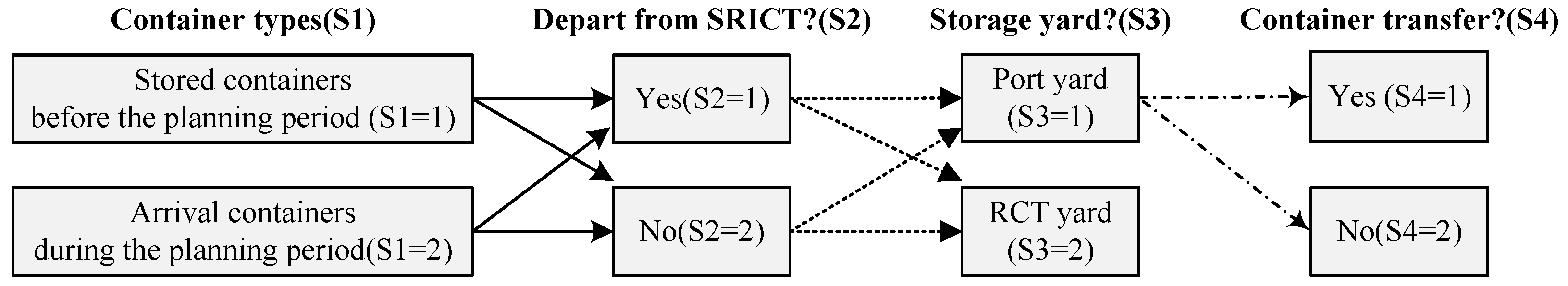
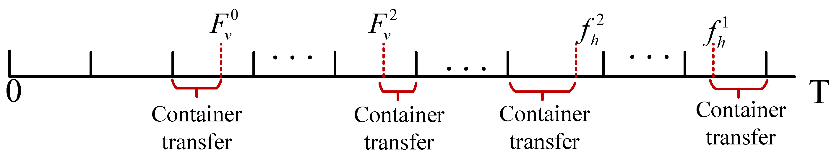
• The handling time continuity of vehicles (ships and trains are hereafter collectively termed “vehicles”) and all possible states of trans-shipment containers are presented. The optimization objectives are designed to align with the long-term strategic goals. Therefore, although this study primarily addresses a single-period resource coordination problem, the proposed framework can be extended to complex multi-period scenarios through decomposition into sequential independent single-period decisions, maintaining its practical applicability for strategic planning purposes.

The remainder of this paper is organized as follows. Section 2 reviews the relevant literature. Section 3 provides a detailed problem description considering shared yards and trucks and develops an MIP optimization model. Section 4 discusses the two-layer APSO-GR algorithm. Section 5 conducts computational experiments to test the performance of the model and algorithm. Section 6 draws conclusions with key findings and future work.

2. Literature Review

2.1. Storage Space Allocation Problem

The storage resource allocation problem encompasses both strategic-level storage space allocation and operational-level storage location assignment. The former involves allocating arriving containers to storage areas, including the yard allocation among multiple terminals and block allocation within one terminal. The storage location assignment refers to allocating containers to specific storage slots defined by three dimensions: bay, row, and tier [5]. This paper focuses on the strategic decision-making level, specifically the yard allocation problem.

The literature directly addressing the yard allocation problem remains limited. Relevant studies were conducted by Lee et al. [6] and Zhen et al. [7], who framed yard allocation as optimal calling terminal selection for arriving ships by minimizing bunker consumption and transportation costs. Hu et al. [8] developed a multi-objective model for yard allocation between seaport and dry port to minimize transportation distance, balance yard utilization, and improve shared space in the dry port. Yard allocation in SRICT concerning two independent parties presents greater complexity and challenges. The most relevant study was investigated by Xie and Song [9], who determined container flows from the port yard and railway buffer to tracks based on train schedules. However, their model ignored critical factors including the handling efficiency of inbound ships, the connection between ships and trains, and resources allocation consideration.

To some extent, block allocation is similar to yard allocation, and related research is relatively mature. The fundamental distinction lies in the yard allocation’s potential involvement of multiple stakeholders with divergent trans-shipment operational paradigms, whereas block allocation operates within a single terminal’s operational framework. Carlo et al. [10] provided comprehensive overviews of block allocation in seaports. Abouelrous et al. [11] determined the block allocation for trans-shipment containers to balance discharge time from unloading vessel to blocks and loading time from blocks to loading vessel. Hu et al. [12] investigated integrated optimization of block allocation and yard crane deployment considering delayed trans-shipment containers. Wang et al. [13] proposed a 3D block allocation problem with the time dimension to decide storage locations for container batches. Cordeau et al. conducted relatively systematic studies on block management, considering traffic intensities to weigh inter-block distances while investigating block allocation within seaports on a whole-ship-container basis [14]. Moreover, they extended the block allocation framework to address yard assignment in an automative trans-shipment terminal [15]. They subsequently established distance thresholds for determining inter-block container transfers within seaports and examined scheduling problems for straddle carriers and multi-trailer systems based on container transfer demand [16].

Driven by the wave of the sharing economy concept, scholars have increasingly focused on storage space sharing in container terminals. Kim et al. [17] classified storage space sharing as logistic facility sharing. He et al. [18] and Tan et al. [19] investigated that each sub-block could be shared among different ships within a port yard. Jin et al. [20] presented the feasibility of shared storage space among different handling companies, proposing a game theory-based approach to allocate storage space and cost among participants. Hu et al. [8] proposed a yard sharing strategy between a seaport and a dry port. Liu et al. [1] conceptualized yard sharing as a mixed storage strategy for railway and road containers within the port yard.

2.2. Truck Allocation Problem

Truck management significantly affects terminal operational efficiency [21]. Plenty of literature has investigated the coordinated scheduling of cranes and trucks [22,23]. Wang et al. [24] presented a two-layer model for truck scheduling problem and truck employment strategy. Karam et al. [21,25] estimated the handling time of ships based on the assigned number of QCs and trucks. Chargui et al. [26] proposed that QC productivity rate is directly correlated with truck deployment. Li et al. [22] formulated time windows according to tidal factors and constructed a joint allocation model of berth-QC-truck. Several works have proposed truck sharing among multiple terminals to overcome resource constraints. Karam et al. [25] developed truck sharing and outsourcing strategies for adjacent terminals. Considering the operation and transfer cost of trucks, Vahdani et al. [27] investigated truck assignment to cranes and truck sharing between adjacent terminals. He et al. [28] discussed the truck-sharing problem to minimize overflowed workloads and transfer costs.

2.3. Container Transshipment Operation

Numerous studies have concentrated on ship-to-ship trans-shipment operation involving only port yard, particularly regarding storage yard management [6,12,22]. Container trans-shipment at intermodal terminals has gradually attracted scholarly attention [2,9,29,30]. Based on the off-dock SRICT layout, Yan et al. [2,30] investigated trans-shipment operation to determine the train schedule template and trans-shipment plan. Considering the turnaround efficiency, Schepler et al. [29] studied the coordinated scheduling of ships, trains, and trucks in a multi-terminal, multi-modal container port.

When arriving and departing terminals differ, inter-terminal transport (i.e., ITT) operations become necessary. The trans-shipment of sea–rail intermodal containers between ports and railways investigated in this research can be attributed to the ITT problem. Heilig and Voß [31] and Hu et al. [32] provided comprehensive reviews of ITT problems. Tierney et al. [33] highlighted that the primary goal of an effective ITT system is reducing transport delays. Schepler et al. [29] studied the ITT problem between multiple ports and RCTs. To reduce the truck traveling costs and container delay, Hu et al. [3,34] investigated the integrated planning for container ITT within the port area and towards the hinterland. Ramadhan et al. [35] determined the truck routing problem of the ITT system to reduce total transportation delay.

2.4. Research Motivation

Existing research on container trans-shipment has predominantly focused on on-dock and off-dock SRICT layouts, while ignoring the most typical seaport–RCT separation layout. Then, several papers have investigated sub-blocks sharing within the port [18,19], and limited research [8,20] has explored yard sharing between seaport and dry ports. However, the coordinated sharing of both yard space and trucks between RCTs and their associated seaports remains an unaddressed research gap. A comparative analysis is presented in

Table 1. Literature on resource allocation in storage yards related to this study.

Literature	Research Area	Resource Allocation	Container Flow	Container Transfer	Objective	Solution Algorithm
Lee et al. (2012) [6]	Multiple sea terminals	Yard and block allocation	Sea containers	Yes	Cost	Two-stage algorithm
Zhen et al. (2016) [7]	Multiple sea terminals	Yard allocation	Sea containers	Yes	Cost	Local branching and PSO *
He et al. (2025) [18]	Seaport yard	Sub-block allocation	Sea containers	No	Yard utilization	PSO
Tan et al. (2024) [19]	Seaport yard	Sub-block allocation	Sea containers	No	Transportation distance and yard utilization	Upper-bound model
Hu et al. (2021) [8]	A seaport yard and a dry port yard	Yard allocation	Sea containers	No	Transportation distance and yard utilization	NSGA-II
Jin et al. (2019) [20]	Multi-terminals	Yard and cost allocation	Storage orders	No	Cost	Game theory
Xie and Song (2018) [9]	SRICT	Yard allocation	Sea–rail containers	Yes	Cost	Optimal strategy
This paper	SRICT	Yard and truck allocation	Sea–rail containers	Yes	Cost and turnaround efficiency	APSO-GR

* Particle swarm optimization.

below. This operational challenge is intricately linked to both ends of sea–rail intermodal transportation, impacting not only the operational capacity of SRICTs but also the coordination efficiency between liner services and freight trains. Given the spatiotemporal constraints of yard operation and storage capacity, coupled with the consideration of accelerating handling efficiency, containers frequently require inter-yard transfer that inevitably increases the yard operational costs. However, the existing literature focuses on the trans-shipment cost minimization while ignoring vehicle turnaround efficiency. The latter is closely related to equipment resource coordination, especially for truck allocation schemes involving highly mobile equipment. To our knowledge, none of the literature addressed the joint allocation optimization of yard space and trucks, so the trans-shipment plan of existing studies is local.

Therefore, this paper fills the research gap by investigating comprehensive resource sharing allocation in the SRICT with the seaport–RCT separation layout. Specifically, we develop a joint optimization framework that simultaneously addresses three critical operational aspects: yard allocation, container transfer, and truck allocation. Departing from the existing literature, our model formulation explicitly balances trans-shipment costs with vehicle turnaround times, offering a more holistic approach to terminal operations optimization.

3. Methodology

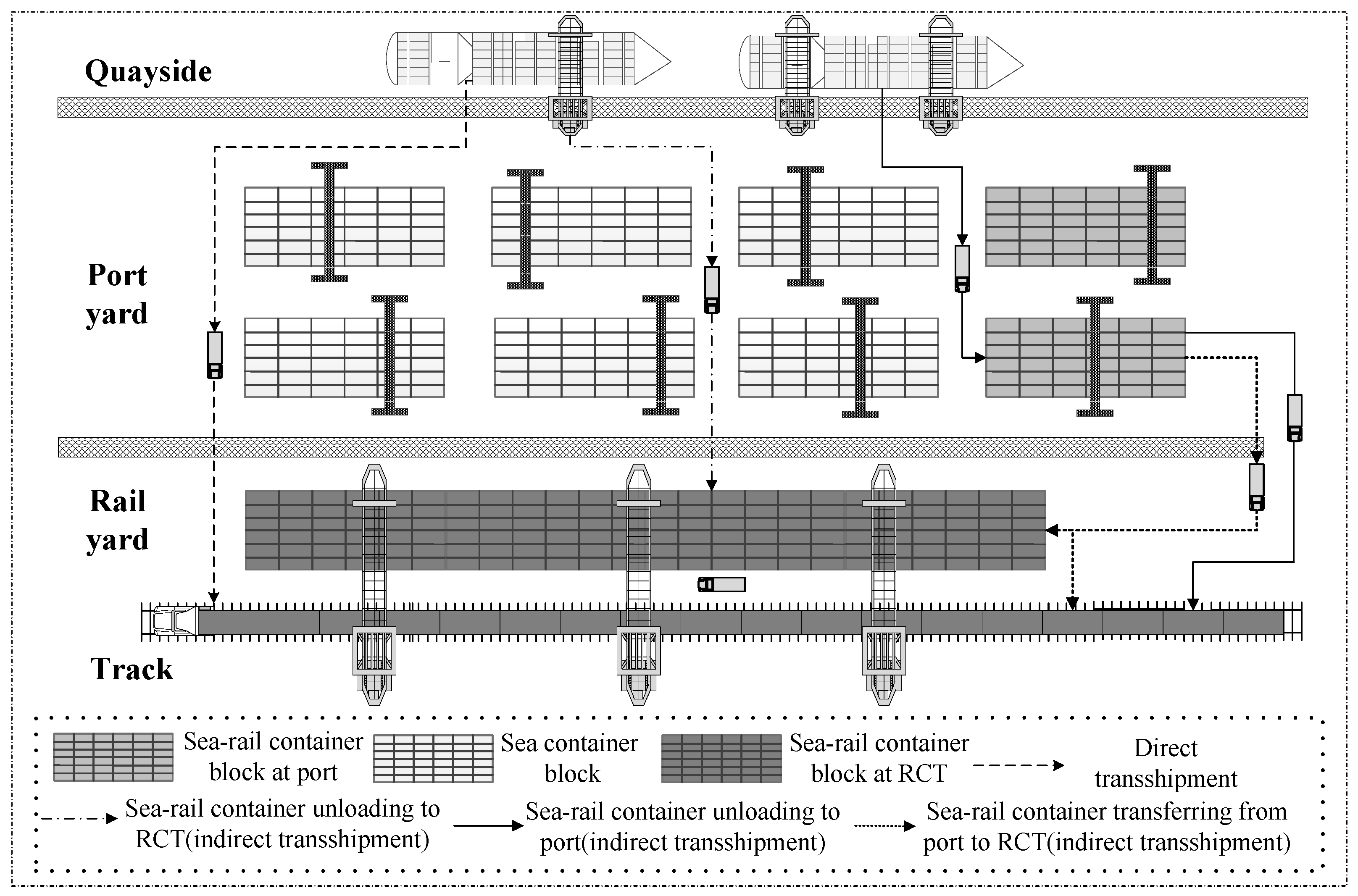
3.1. Problem Description

In traditional storage form, inbound containers are first unloaded from ships to the port yard and subsequently transported to rail tracks when trains arrive. This practice frequently leads to port yard congestion and potential train delays. Based on the shared storage space form, arriving containers could be flexibly stored in either the port yard or RCT yard. Operators can reasonably arrange yards by evaluating storage capacity, handling efficiency, and equipment availability. Consequently, three trans-shipment modes are established for inbound containers: (1) ship-to-port yard, (2) ship-to-RCT yard, and (3) ship-to-port yard-to-RCT yard.

Mode 1 is the same as the traditional form, which boasts high ship unloading efficiency but compromising train loading efficiency due to long-distance transportation. In Mode 2, QCs unload containers from arrived ships onto trucks for horizontal transportation to the RCT yard. Upon train arrival, gantry cranes (i.e., GCs) subsequently load containers from the RCT yard onto the train. Mode 2 offers superior loading efficiency at the expense of reduced ship unloading efficiency. Mode 3 has container transfer operation from the port yard to the RCT yard by trucks, reducing handling distances. Therefore, the storage pressure and cost between port and RCT and handling efficiencies between ships and trains have been balanced. All three modes require QC unloading and GC loading operations exhibiting distinct utilization patterns for trucks, yard cranes (i.e., YCs), and GCs is inconsistent. Figure 2 maps five imported container flows to three trans-shipment modes. The flow of import trans-shipment containers from the RCT yard to the port yard produces two invalid transfers that violate the practical business. Figure 3 systematically defines all 12 possible operational states based on four key attributes.

Given the strategic nature of resource allocation decisions, the chosen level of granularity is the batch level. A batch corresponds to a set of containers with the same attributes. For arriving containers arriving during the planning period, a batch refers to a set of containers unloaded from the same ship and later loaded onto the same train. For stored containers before the planning period, a batch refers to a set of containers stored in a port yard and loaded onto the same train, or stored in a RCT yard and loaded onto the same train. We employ batches instead of container units to reduce the model complexity [8,14,29]. In practice, trans-shipment operations at SRICTs occur on a continuous timeline. To reduce computational complexity while maintaining alignment with real-world operational requirements, we use discrete time intervals to represent actual continuous arrival, handling, and departure times of ships and trains. We will discuss the following three sub-problems based on the seaport–RCT separation layout.

• Yard allocation: For arriving trans-shipment batches during the planning horizon, decide which yard containers are stored, RCT yard or port yard.
• Container transfer: Due to limited storage capacity and the turnaround efficiency of vehicles, containers may transfer from the port yard to the RCT yard. We conduct the quantity and time of container transfer. This sub-problem is intended for the import trans-shipment batches arriving and stored in the port during the planning horizon and pre-existing batches stored in the port before the planning horizon.
• Truck allocation: Allocate trucks for ships, trains, and container transfer within specified fleet constraints.

3.2. Model Formulation

3.2.1. Model Assumptions

Several assumptions are adopted for the mathematical formulation:

(1) All containers are FEUs (i.e., forty-foot equivalent units).

(2) The arrival schedules of ships and trains are known in advanced by referring to timetables.

(3) The total exchange container volume between ships and trains is predetermined.

(4) The handling efficiency under the configuration of cranes and trucks is known.

3.2.2. Notations

(1) Sets and Parameters

T: Set of time intervals of the planning horizon, $t\in T=\{1,\dots ,|T\left|\right\}$

V: Set of ships, $v\in V$

H: Set of trains, $h\in H$

B: Set of container batches, $b\in B$

R: Set of yards, $r\in R=\{1,2\}$, and 1 and 2 represent the port yard and RCT yard

S: Set of vehicle, including ships and trains, $s\in S=\{1,2,\dots ,|S\left|\right\}$ and $S=V\cup H$

$\mathrm{\Gamma }$: Set of truck number, $n\in \mathrm{\Gamma }=\{1,\dots ,|\mathrm{\Gamma }\left|\right\}$

$m_v$: Index of QC’s number allocated to ship v

g: Index of GC’s number

$F_v^0$: Planned start time of unloading trans-shipment containers for ship v

$f_h^0$: Planned start time of loading trans-shipment containers for train h

$P_{bv}$: Set to 1 if batch b is unloaded from ship v, and 0 otherwise

$p_{br}$: Set to 1 if batch b is stored in the yard r before planning horizon, and 0 otherwise

$q_{bh}$: Set to 1 if batch b is loaded to train h, and 0 otherwise

${\mathrm{\Omega }}_r^1$: Storage capacity of yard r

${\mathrm{\Omega }}_{tr}^2$: Handling capacity of yard r at interval t

$N_b$: Number of containers in batch b

$c^1$: Unit handling cost of the YC

$c^2$: Unit handling cost of the GC

$c^3$: Unit handling cost of the QC

$c_r$: Unit storage cost of yard r

$c^4$: Unit usage cost of trucks

$w_s$: Weight of turnaround time for vehicle s

$\tau$: Hours in a planning interval

M: A sufficiently large positive number

${\rho }_{m_v}^{nr}$: Average number of containers handled to yard r with n trucks per QC and per interval when the number of QCs allocated to ship v is $m_v$

${\pi }_g^n$: Average number of containers for handling with n trucks per GC and per interval when the number of GCs allocated to train is g

${\psi }_s$: Maximum truck number allocating to vehicle s

(2) Decision variables

$x_{br}$: =1 if batch b is loaded to train from yard r; =0 otherwise

$y_{bt}$: =1 if batch b is transferred to RCT yard during interval t; =0 otherwise

${\xi }_{vn}$: =1 if allocated number of trucks to ship v for unloading is n; =0 otherwise

${\zeta }_{hn}$: =1 if allocated number of trucks to train h for loading is n; =0 otherwise

${\sigma }_{tn}$: =1 if allocated number of trucks to transfer containers during interval t is n; =0 otherwise

(3) Derived variables

$z_{br}$: =1 if arriving batch b is unloaded to terminal r; =0 otherwise

${\chi }_{ts}$: Allocated number of trucks to vehicle s in interval t

$F_v^r$: Finish time for ship v unloading containers to yard r

$f_h^r$: Finish time for train h loading containers from yard r

${\alpha }_{vr}^t$: Number of containers unloading from ship v to yard r in interval t

${\beta }_{rh}^t$: Number of containers loading from yard r to train h in interval t

$Q_t^r$: Number of containers storing in yard r at the end of interval t

$C_b^1$: Unit storage cost of batch b

$C_b^2$: Unit usage cost of batch b

$C_b^3$: Unit handled cost of batch b

3.2.3. Formulation

$$min{Z}_0=\lambda Z_1+(1-\lambda )\omega Z_2$$

(1)

$$Z_1=\sum _{b\in B}\sum _{i\in \{1,2,3\}}{N}_b{C}_b^i$$

(2)

$$Z_2=\left[\sum _{v\in V}{w}_v(F_v^2-F_v^0)+\sum _{h\in H}{w}_h(f_h^1-f_h^0)\right]3600\tau$$

(3)

Equation (1) is the objective function, including container operational cost in Equation (2) and the weighted vehicle turnaround time in Equation (3). The difference in truck transportation cost from the quayside to rail tracks is small, so we ignore it and focus on truck usage cost varied with trans-shipped modes. Considering the differences in operating costs and time sensitivity, a weighting coefficient $w_s$ is introduced to reflect the priority of vehicles [29]. To reconcile the dimension inconsistency between these two indicators, we introduce balancing parameter $\omega$. Moreover, we used the weight $\lambda$ to measure the preference of indicators to the SRICT operators.

$$\begin{array}{cc}\hfill & C_b^1=\sum _{t\in T}{y}_{bt}{c}_1\left[x_{b1}(t-\sum _{v\in V}{P}_{bv}{F}_v^0)+p_{b1}{c}_{1}t\right]+\sum _{r\in R}\sum _{h\in H}{z}_{br}{c}_r{q}_{bh}\left[p_{br}{f}_h^1+x_{br}(f_h^1-\sum _{v\in V}{P}_{bv}{F}_v^0)\right]\hfill \\ \hfill & \sum _{t\in T}(x_{b1}+p_{b1})y_{bt}{c}_2\left[\sum _{h\in H}{q}_{bh}(f_h^1-t)+(1-\sum _{h\in H}{q}_{bh})(\left|T\right|-t)\right]+\hfill \\ \hfill & (1-\sum _{h\in H}{q}_{bh})c_2\left[p_{b1}\left|T\right|+\sum _{r\in R}{x}_{br}(\left|T\right|-\sum _{v\in V}{P}_{bv}{F}_v^0)\right]+\hfill \\ \hfill & (1-\sum _{h\in H}{q}_{bh})(1-\sum _{t\in T}{y}_{bt})c_1\left[p_{b1}\left|T\right|+\sum _{r\in R}{x}_{br}(\left|T\right|-\sum _{v\in V}{P}_{bv}{F}_v^0)\right]\hfill \end{array}$$

(4)

$$C_b^2=\sum _{r\in R}{c}^4{x}_{br}+\sum _{t\in T}{c}^4{y}_{bt}+c^4{z}_{b1}$$

(5)

$$C_b^3=\sum _{r\in R}{c}^3{x}_{br}+\sum _{r\in R}{c}^2{z}_{br}+\sum _{t\in T}(c^1+c^2)y_{bt}+c^1{x}_{b1}+c^2{x}_{b2}+c^1{z}_{b1}$$

(6)

$$\sum _{r\in R}{x}_{br}=1-\sum _{r\in R}{p}_{br},\forall b\in B$$

(7)

$$\sum _{t\in T}{y}_{bt}\le 1,\forall b\in B$$

(8)

$$\sum _{t\in T}{y}_{bt}\le p_{br}+x_{br},\forall b\in B,r=1$$

(9)

$$p_{br}+x_{br}\le 1-\sum _{t\in T}{y}_{bt},\forall b\in B,r=2$$

(10)

$$t{y}_{bt}\ge p_{br},\forall b\in B,r=1,t\in T$$

(11)

$$t{y}_{bt}+M(1-x_{br})\ge \sum _{v\in V}{P}_{bv}\lceil F_v^1\rceil +1,\forall b\in B,r=1$$

(12)

$$t{y}_{bt}\le M(1-x_{br})+\sum _{h\in H}{q}_{bh}\lfloor f_v^0\rfloor -1,\forall b\in B,r=1$$

(13)

$$z_{b1}+M\left[1-(x_{b1}+p_{b1})\sum _{h\in H}{q}_{bh}+\sum _{t\in T}{y}_{bt}\right]\ge 1,\forall b\in B$$

(14)

$$z_{b2}+M\left[2-(x_{b1}+p_{b1})\sum _{h\in H}{q}_{bh}-\sum _{t\in T}{y}_{bt}\right]\ge 1,\forall b\in B$$

(15)

$$z_{b2}+M\left[1-(x_{b2}+p_{b2})\sum _{h\in H}{q}_{bh}\right]\ge 1,\forall b\in B$$

(16)

$$Q_t^r=\sum _{b\in B}{p}_{br}{N}_b,\forall r\in R,t=0$$

(17)

$$Q_t^1=Q_{t-1}^1+\sum _{v\in V}{\alpha }_{v1}^t-\sum _{h\in H}{\beta }_{1h}^t-\sum _{b\in B}{y}_{bt}{N}_b,\forall t\in T$$

(18)

$$Q_t^2=Q_{t-1}^2+\sum _{v\in V}{\alpha }_{v2}^t-\sum _{h\in H}{\beta }_{2h}^t,t=1$$

(19)

$$Q_t^2=Q_{t-1}^2+\sum _{v\in V}{\alpha }_{v2}^t+\sum _{b\in B}{y}_{b(t-1)}{N}_b-\sum _{h\in H}{\beta }_{2h}^t,\forall t\in T,t\ge 2$$

(20)

$$Q_t^r\le {\mathrm{\Omega }}_r^1,\forall r\in R,t\in T$$

(21)

$$\sum _{t\in T}{\alpha }_{vr}^t=\sum _{b\in B}{N}_b{x}_{br}{P}_{bv},\forall r\in R,v\in V$$

(22)

$$\sum _{t\in T}{\beta }_{rh}^t=\sum _{b\in B}{q}_{bh}{N}_b{z}_{br},\forall h\in H,r\in R$$

(23)

$$\sum _{v\in V}{\alpha }_{vr}^t+\sum _{h\in H}{\beta }_{rh}^t+\sum _{b\in B}{y}_{b(t-r+1)}{N}_b\le {\mathrm{\Omega }}_{tr}^2,\forall t\in T,r\in R$$

(24)

$${\alpha }_{vr}^t\le \sum _{n\in \mathrm{\Gamma }}{\xi }_{vn}{\rho }_{m_v}^{nr},\forall t\in T,v\in V,r\in R$$

(25)

$${\beta }_{rh}^t\le \sum _{n\in \mathrm{\Gamma }}{\zeta }_{hn}{\pi }_g^n,\forall t\in T,h\in H,r\in R$$

(26)

$${\chi }_{tv}=n{\xi }_{vn},\lceil F_v^0\rceil \le t\le \lceil F_v^2\rceil ,n\in [0,min(\left|\mathrm{\Gamma }\right|,{\psi }_v)],v\in V$$

(27)

$${\chi }_{th}=n{\zeta }_{hn},\lceil f_h^2\rceil \le t\le \lceil f_h^1\rceil ,n\in [0,min(\left|\mathrm{\Gamma }\right|,{\psi }_h)],h\in H$$

(28)

$$\sum _{s\in V\cup H}{\chi }_{ts}+\sum _{n\in \mathrm{\Gamma }}n{\sigma }_{tn}\le \left|\mathrm{\Gamma }\right|,\forall t\in T$$

(29)

$$F_v^r\ge F_v^{r-1}+\sum _{b\in B}\sum _{n\in \mathrm{\Gamma }}{\xi }_{vn}{P}_{bv}{x}_{br}{N}_b/{\rho }_{m_v}^{nr},\forall v\in V,r\in R$$

(30)

$$f_h^2\ge f_h^0+\sum _{b\in B}{q}_{bh}{N}_b{z}_{b2}/{\pi }_g^0,\forall h\in H$$

(31)

$$f_h^1\ge f_h^2+\sum _{b\in B}\sum _{n\in \mathrm{\Gamma }}{\zeta }_{hn}{q}_{bh}{N}_b{z}_{b1}/{\pi }_g^n,\forall h\in H$$

(32)

$$(x_{br},y_{bt},{\xi }_{vn},{\zeta }_{hn},{\sigma }_{tn},z_{br})\in \{0,1\},\forall b\in B,r\in R,t\in T,n\in \mathrm{\Gamma }$$

(33)

$$({\chi }_{ts},{\alpha }_{vr}^t,{\beta }_{rh}^t,Q_t^r)\in \mathbb{N},\forall t\in T,s\in V\cup H,h\in H,v\in V$$

(34)

$$(F_v^r,f_h^r,C_b^i)\ge 0,\forall v\in V,r\in R,h\in H,b\in B,i\in \{1,2,3\}$$

(35)

Equations (4)–(6) calculate the handling cost, truck usage cost, and storage cost, with the detailed computation methodology provided in Appendix A. Aligned with all operational states illustrated in Figure 3, we consider the differences in handling, transportation, and storage operations between the ports and the RCT. Equation (7) indicates that each arriving containers must be allocated to exactly one yard. Equation (8) limits at most one transfer for each batch. Equations (9) and (10) restrict that only batches stacked in the port yard may transfer, excluding stored batched in the RCT yard. For the batch stored in the port yard before the planning horizon, Equations (11) and (13) confine the transfer time to no less than one and no later than the start loading time of the train. For arriving batch stored in the port during the planning horizon, Equations (12) and (13) limit the transfer time to no earlier than the finish time of ship unloading and no later than the start time of train loading. Equations (14)–(16) define the derived variable by decision variables $x_{br}$ and $y_{bt}$. Equations (17)–(20) are recursion for the storage quantity and the expression for the inflow and outflow of containers. Equation (21) limits the storage capacity. Equations (22) and (23) define handling volumes through variables. Equation (24) limits yard handling capacity. Equations (25) and (26) illustrate that handling volumes are limited by truck transport capacity. Equations (27) and (28) indicate the relationship between variables related to truck allocation. Specifically, trucks would be allocated to vehicles only when they have transportation needs. Equation (29) limits the available trucks number. Equations (30)–(32) represent the completion time of vehicles. Generally, the SRICT adopts “nearest principle” for handling. During ship unloading process, the batch allocated to the port yard is unloaded first and then to the RCT yard, while train loading process follows the reverses sequence. Equations (33)–(35) define variables.

3.2.4. Model Validation

To verify the correctness of the model, we employ the CPLEX solver to obtain solutions. Specific parameters refer to Section 5.1. The formulation presented in Section 3.2 constitutes a nonlinear MIP model, and Appendix B gives its linearization process. The linearization increases model complexity by introducing high-dimensional variables and additional constraints. We set the computational (i.e., CPU) time limit of 7200 s for CPLEX solver.

Table 2. Solution results by CPLEX solver.

Instance	${\mathit{Z}}_1$	${\mathit{Z}}_2$/s	${\mathit{Z}}_0$	CPU/s
I1	5209.7	9288.6	4879.7	236
I2	5906.7	7248.5	4854.9	577
I3	7011.4	10,232.0	5773.7	1328
I4	26,067.4 *	10,392.7 *	25,111.9 *	7200
I5	—	—	—	7200

* Satisfactory solutions obtained by CPLEX at 7200 s (indicating that CPLEX cannot obtain best solutions within 7200 s).

shows results. The value of parameter $\omega$ is also determined by Equation (42), meaning it adopts the same value obtained from the APSO-GR algorithm in Section 5.2. This approach is necessary because the dimensional standards of indicators $Z_1$ and $Z_2$ cannot be predetermined. Conducting prior algorithmic experiments provides a scientifically justified value while facilitating subsequent validation of the algorithm’s effectiveness.

Exact solutions for small size instances I1∼I3 can be obtained within 7200 s by the CPLEX solver, confirming the MIP model’s solvability and correctness. However, computational complexity grows exponentially with problem size. For medium- and large-scale instances I4∼I12, the CPLEX fails to obtain exact solutions within 7200 s. Notably, for instances I5∼I12, feasible solutions cannot be obtained within 7200 s by the CPLEX. Therefore, we develop a dedicated algorithm to solve the comprehensive problem.

4. Solution Algorithm

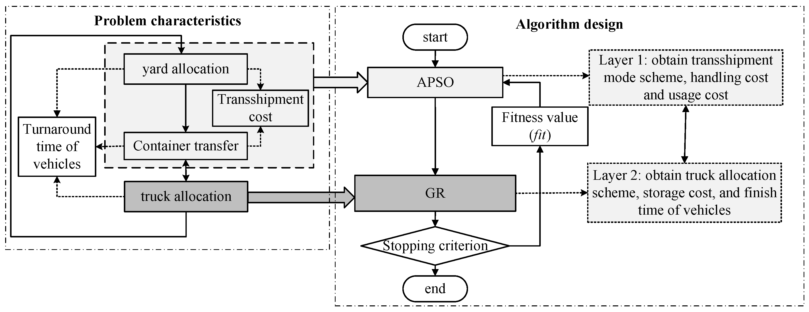
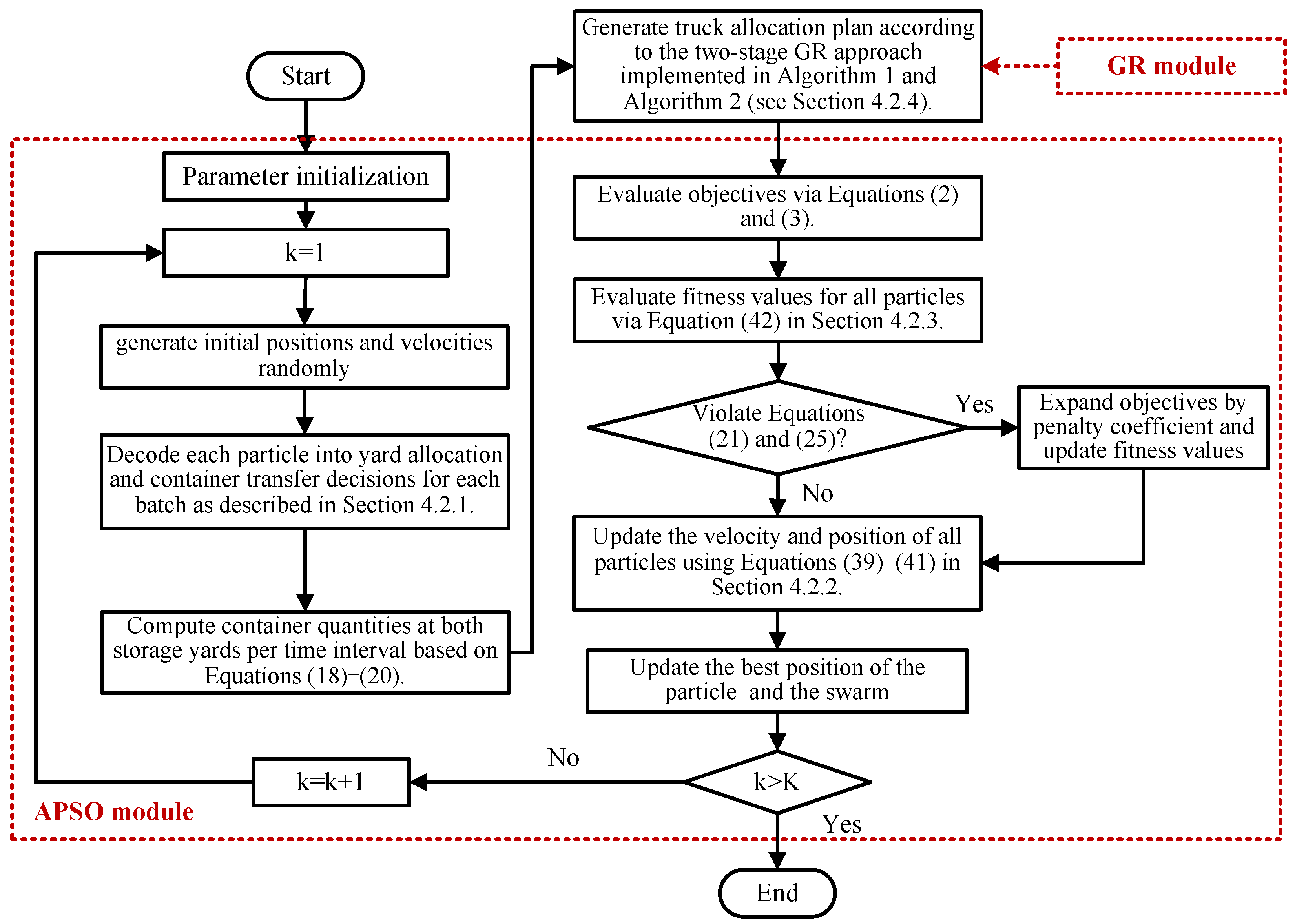
4.1. Algorithm Framework

The joint allocation problem is a two-level and two-way correlation optimization problem, as indicated in Figure 4. Yard allocation is the basis for container transfer. Both decisions require trucks for horizontal transportation. All sub-problems affect vehicle turnaround. Faster ship turnaround occurs if containers prefer to unload to the port yard, while accelerated train turnaround is achieved if containers are headed towards unloading or transferring to the RCT yard. The higher the number of trucks allocated, the faster the turnaround efficiency. However, the number of trucks assigned is limited by the total quantity availability and operational capabilities. Container transfer increases transit costs but accelerates vehicle turnaround.

Lee et al. [6] regarded the yard allocation problem as a simple space–time network, where the temporal dimension represents transfer time and the spatial dimension reflects storage yards. Both Lee et al. [6] and Zhen et al. [7] demonstrated that the yard allocation problem is NP-hard. Truck allocation is a mechanical assignment problem that has been proved NP-hard [28]. The joint allocation problem of shared resources in SRICTs can be demonstrated as NP-hard through polynomial-time reduction to the classical Bin Packing problem [36]. By establishing the following mapping relationships: assuming unlimited capacity for each storage yard, the item volumes in Bin Packing correspond to the storage demands of containers, the number of bins maps to the limit on the number of storage yards, and the dependency between the number of containers allocated to a yard and the required number of trucks is defined to couple the capacity constraints of Bin Packing with the transportation resource constraints. This mapping process only requires iterating through all n items (containers) and m bins (yards) with a time complexity of $O(m+n)$, along with directly calculating truck demands (in $O\left(1\right)$ per yard), resulting in an overall linear time complexity that is polynomially bounded. Therefore, since the joint allocation problem of shared resources can be reduced to the NP-hard Bin Packing problem in polynomial time, it follows that the former is also NP-hard. As shown in Table 2, it is inefficient to obtain optimal solutions by commercial solvers or exact algorithms in polynomial time unless P = NP [37]. Therefore, based on the characteristics of the problem, we propose a two-layer hybrid heuristic algorithm, namely APSO-GR algorithm, to obtain solutions.

The overall framework of the APSO-GR algorithm is shown in Figure 4. The first layer utilizes the APSO algorithm to solve yard allocation and container transfer decisions. The trans-shipment modes for each batch are determined, after which $C_b^2$ and $C_b^3$ can be calculated. According to these trans-shipment results, the second layer employs GR to decide the truck allocation scheme. The obtained fitness value is returned to the APSO layer. Then, the down-top iteration is performed. The APSO-GR algorithm employs a bi-directional layer-by-layer iteration process, first top-down then bottom-up, to obtain global optimization. The maximum number of iterations is set as the termination condition. The complete procedural workflow of the APSO-GR algorithm is detailed in Figure 5.

In recent years, the PSO algorithm, wolf pack algorithm (i.e., WPA), genetic algorithm, etc., have been effectively applied to solve optimization problems. This study prioritizes PSO as the first-layer algorithm due to its inherent advantages. Firstly, PSO exhibits superior optimization capabilities for the continuous variable problem. Assuming symbol–number coding is used in the first layer, a three-dimension coding framework needs to be established for the selected storage yard, whether to transfer, and the transfer time. The symbol encoding introduces greater complexity and randomness to solutions generation and updating. Therefore, we adopt float continuous encoding for binary variables $x_{br}$ and $y_{bt}$. Secondly, PSO has demonstrated effectiveness and been widely applied in port operation management, including yard allocation [7], sub-block allocation [18], and crane scheduling [38]. Thirdly, PSO’s simplicity and low computational cost enhance its suitability for large-scale scenarios. Finally, PSO requires fewer parameters, simplifying the search process and enabling faster adaptation and implementation.

4.2. Algorithm Tactics

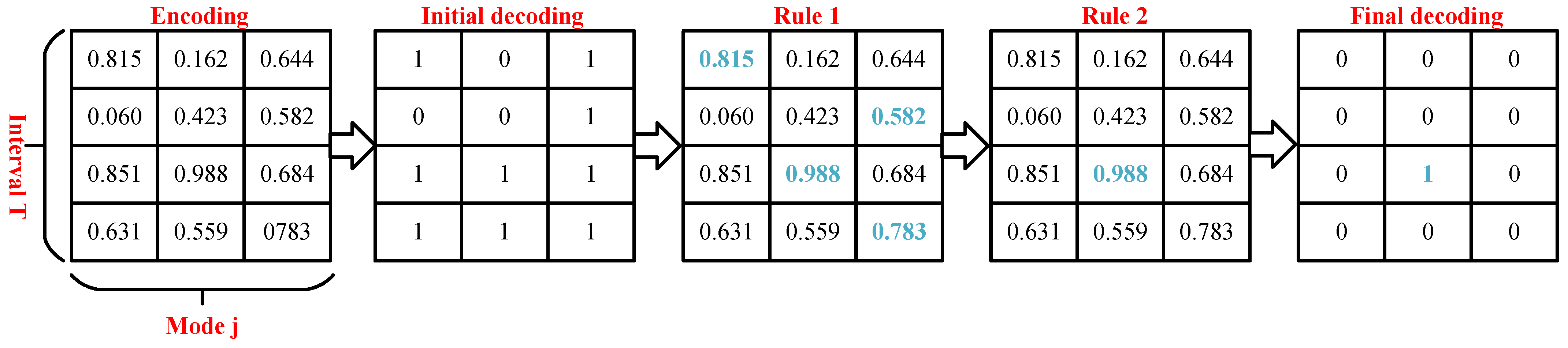
4.2.1. Encoding and Decoding Strategy

We define the binary variable $X_{bt}^j$ to reflect decision variables $x_{br}$ and $y_{bt}$ in Equations (36) and (37). If batch b chooses the trans-shipment mode j of the sharing yard form in Figure 2, $X_{bt}^j=1$; otherwise, $X_{bt}^j=0$, where $j\in \{1,2,3\}$.

The position and velocity of particle i in iteration k are defined by $U_{ki}=\left\{u_{btj}^{ki}\right\}$ and $V_{ki}=\left\{v_{btj}^{ki}\right\}$, respectively. We map the continuous particle space $u_{btj}^{ki}$ to the discrete problem space $X_{bt}^j$ with Equation (38).

$$\left\{\begin{array}{c}{x}_{b1}=1\&{\displaystyle \sum _{t\in T}}{y}_{bt}=0\to X_{b0}^1=1\hfill \\ x_{b2}=1\&{\displaystyle \sum _{t\in T}}{y}_{bt}=0\to X_{b0}^2=1\hfill \\ x_{b1}=1\&y_{bt}=1\to x_{bt}^3=1\hfill \end{array}\right.\hspace{1em}\forall b\in B,t\in T$$

(36)

$$\left\{\begin{array}{c}{p}_{b1}=1\&{\displaystyle \sum _{t\in T}}{y}_{bt}=0\to X_{b0}^1=1\hfill \\ p_{b1}=1\&y_{bt}=1\to X_{bt}^3=1\hfill \end{array}\right.\hspace{1em}\forall b\in B,t\in T$$

(37)

$$X_{bt}^j=\left\{\begin{array}{c}1if{u}_{btj}^{ki}>0.5\hfill \\ 0if{u}_{btj}^{ki}\le 0.5\hfill \end{array}\right.$$

(38)

A trans-shipment mode for batch b must meet the constraint of ${\displaystyle \sum _{j\in \{1,2,3\}}}{\displaystyle \sum _{t\in T}}{X}_{bt}^j=1$ and comply with Equations (11)–(13) on transfer time. We design two heuristic rules for the encoding and decoding strategy, and a sample example is shown in Figure 6.

Rule1: For any interval t and batch b, if multiple modes j satisfy $X_{bt}^j=1$, select the plan $j^{*}$ with maximum value of positions; that is, $j^{*}=argma{x}_j\left(u_{btj}^{ki}\right)$.

Rule2: For any batch b, if multiple intervals t satisfy $X_{bt}^j=1$, select the plan j corresponding to the interval $t^{*}$ with the largest value of positions; that is, $t^{*}=argma{x}_t\left(u_{btj}^{ki}\right)$, while meeting the preliminary transfer time determination. Equations (11)–(13) define the transfer time range of the batch as $\left[\lceil F_v^1\rceil +1,\lfloor f_h^0\rfloor -1\right]$. Since $\lceil F_v^1\rceil$ is the variable to solve, it needs to be replaced by known parameters. We reasonably expand the transfer time to $\left[\lceil F_v^0\rceil +1,\lfloor f_h^0\rfloor -1\right]$. Then, when evaluating the fitness value, transfer time violating Equations (11)–(13) are eliminated by applying a penalty coefficient ℓ that expands the objective function by ℓ times based on prior experiments.

4.2.2. Adaptively Updating of Velocity and Position

Equations (39) and (40) are the velocity and position updating method. The non-negative $w^k$ represents the inertia factor; K denotes the maximum iteration count; $l_1$ and $l_2$ are learning factors within [0,4], typically set to 2 [7]; $r_1$ and $r_2$ are random numbers uniformly distributed in (0,1); $PbBes{t}_{btj}^{ki}$ represent the best position of particle i along dimension $(b,t,j)$ up to iteration k; $gBes{t}_{btj}^k$ is the best position of the entire swarm along dimensions $(b,t,j)$ up to iteration k.

$$v_{btj}^{(k+1)i}=w^k{v}_{btj}^{ki}+l_1{r}_1(PbBes{t}_{btj}^{ki}-u_{btj}^{ki})+l_2{r}_2(gBes{t}_{btj}^k-u_{btj}^{ki})$$

(39)

$$u_{btj}^{(k+1)i}=u_{btj}^{ki}+v_{btj}^{(k+1)i}$$

(40)

The dynamic inertia factor outperforms fixed values by adaptively balancing the global and local optimization. We adopt an adaptively decreasing weight strategy to adjust the inertia factor based on particle swarm fitness values in Equation (41). When particle swarm diversity is high, a larger inertia factor is assigned to enhance global search capabilities; when the diversity is low, a smaller inertia factor is used to strengthen local search. This adaptive mechanism maintains a balanced exploration–exploitation trade-off throughout the search process. Parameters $w^{ini}$ and $w^{end}$ represent the initial weight at iteration 1 and the final weight at maximum iteration K, with typical values of 0.9 and 0.4, respectively. Values $fi{t}_{best}\left(k\right)$ and $fi{t}_{worst}\left(k\right)$ denote the best fitness value and the worst fitness value in the current iteration k, respectively.

$$w^k=w^{end}+(w^{ini}-w^{end}){\displaystyle \frac{fi{t}_{best}\left(k\right)-fi{t}_{worst}\left(k\right)}{fi{t}_{best}\left(k\right)+fi{t}_{worst}\left(k\right)}}$$

(41)

4.2.3. Fitness Function

By calculating the mean value of $Z_1$ and $Z_2$ for the whole swarm in each iteration, we determine the balance coefficient $\omega$ using the ratio of their mean values. The obtained fitness function is given in Equation (42).

$$\left\{\begin{array}{c}fitness=Z_0=\lambda Z_1+(1-\lambda )\omega Z_2\hfill \\ \omega =\overline{Z_1\left(k\right)}/\overline{Z_2\left(k\right)}\hfill \end{array}\right.$$

(42)

4.2.4. GR for Truck Allocation

We design a two-stage GR approach to allocate limited trucks. The first stage in Algorithm 1 allocates trucks to sorted vehicles based on arrival time according to freight ratios of handling containers, which conforms to the basic principle of demand-driven provisioning in real-world operations. The second stage in Algorithm 2 utilizes remaining truck capacity for container transfer. The specific implementation follows these stages.

Algorithm 1 The first stage pseudocode: allocate trucks for vehicles

Input:  $ST$: the beginning time of ships’ unloading containers and trains’ loading containers stored in the port, $ST=\{F_v^0,f_h^2,v\in V,h\in H\}$; $XL$: the container number of ships’ unloading to two yards and trains’ loading from the port yard, $XL=\{{\displaystyle \sum _{t\in T}}{\alpha }_{vr}^t,{\displaystyle \sum _{t\in T}}{\beta }_{1h}^t,v\in V,h\in H,r\in R\}$; $\left|\mathrm{\Gamma }\right|$, $\left|S\right|$, and ${\psi }_s$ refer to Section 3.2.2. Output:  $chr$: truck allocation scheme for vehicles, $chr=\{n{\xi }_{vn},n{\zeta }_{hn},v\in V,h\in H\}$; $FT$: Handling completion time of vehicles, $FT=\{F_v^2,f_h^1,v\in V,h\in H\}$; $Tchr$: truck allocation scheme for each vehicle in each interval, $Tchr=\{{\chi }_{ts},t\in T,s\in S\}$. 1: sort $ST$ in ascending order, and set the order index with notation ℓ 2: $chr\left(\mathcal{l}\left(1\right)\right)\Leftarrow min(\left|\mathrm{\Gamma }\right|,{\psi }_{\mathcal{l}\left(1\right)})$ when $XL\left(\mathcal{l}\left(1\right)\right)\ge 0$. 3: compute $FT$ of vehicle $\mathcal{l}\left(1\right)$ according to Equations (30)–(32) 4: $Tchr\left(\left(\mathcal{l}\right(1),ST:FT\right)\Leftarrow chr$ 5: for $m\in \left\{\mathcal{l}\right(2),\dots ,\mathcal{l}(\left|S\right|\left)\right\}$do 6:    if $XL\left(m\right)>0$ then 7:      $ind\Leftarrow ind\cup \left\{m^{*}\right\}$ when $ST\left(m^{*}\right)\le \lceil ST\left(m\right)\rceil \le FT\left(m^{*}\right)$ for all $m^{*}\in \{1,\dots ,m-1\}$ 8:      /*Compute the freight ratios $ft$ when $ind\ne ⌀$ 9:      $ft\left(e\right)\Leftarrow XL(1,e)/{\displaystyle \sum _{e\in ind\cup \left\{m\right\}}}XL(1,e)$, for all $e\in ind\cup \left\{m\right\}$ 10:      $chr\left(e\right)\Leftarrow min\left\{max\left[round\left(\right|\mathrm{\Gamma }\left|ft\right(e\left)\right),1\right],{\psi }_m\right\}$, for all $e\in ind\cup \left\{m\right\}$ 11:      compute $FT$ and $Tchr$ of vehicles with index e, for all $e\in ind\cup \left\{m\right\}$ 12:      /*Repair procedure for Scenario 1 13:      for $t\in \left\{1,\dots ,\lceil FT\left(m\right)\rceil \right\}$ do 14:         sum the number of trucks of each interval denoted as $STchr\left(t\right)$ 15:         $in{d}^{\prime }\Leftarrow in{d}^{\prime }\cup k^{*}$ when $STchr\left(t\right)>\left|\mathrm{\Gamma }\right|$ and $Tchr(k^{*},t)>0$ 16:         reset $chr$, $FT$, and $Tchr$ of vehicles in set $in{d}^{\prime }$ according to freight ratio when $in{d}^{\prime }\ne ⌀$ 17:      end for 18:    else 19:      /* Means that vehicle m is a train, and the batches carried are all stored in the RCT yard 20:      compute completion time $FT$ and $Tchr$ of vehicles m. 21:    end if 22: end for

Algorithm 2 The second stage pseudocode: allocate trucks to container transfer

Input:  $CT$: Number of containers to be transferred, $CT=\left\{{\displaystyle \sum _{b\in B}}{\displaystyle \sum _{t\in T}}{y}_{b}t{N}_b\right\}$; Notations T and $\mathrm{\Gamma }$ refer to Section 3.2.2; Notations $ST,chr,FT,Tchr$ and $STchr$ refer to Algorithm 1. Output:  $Zchr$: truck allocation scheme for container transfer, $Zchr=\{n{\sigma }_{tn},t\in T,n\in N\}$; Notations $chr,FT,Tchr$, and $STchr$ refer to Algorithm 1. 1: compute remaining transportation capacity at each interval and denote as $Rcap$. 2: for $t\in T$ do 3:     $done\Leftarrow 0$ 4:     while $done=0$ do 5:         if $Rcap\left(t\right)<CT\left(t\right)$ then 6:            if $\left|\mathrm{\Gamma }\right|-STchr\left(t\right)>0$ then 7:                $Zchr\left(t\right)\Leftarrow Zchr\left(t\right)+1$, $done\Leftarrow 0$, and recompute $STchr\left(t\right)$ 8:            else 9:                find the maximal $Tchr(k^{*},t)$ with $k^{*}$ for all the vehicle 10:              $Zchr\left(t\right)\Leftarrow Zchr\left(t\right)+1$, $done\Leftarrow 0$ when $Tchr(k^{*},t)>1$ 11:              recompute $FT$, $chr$ and $Tchr$ of vehicle $k^{*}$, and recompute $STchr\left(t\right)$ 12:              /* Repair procedure for Scenario 2 13:              if the original completion time $F{T}^{\prime }\left(k^{*}\right)\le FT\left(k^{*}\right)$ then 14:                  for $tt\in \left\{\lceil F{T}^{\prime }\left(k^{*}\right)\rceil +1,\dots ,\rceil FT(k^{*}\rceil )\right\}$ do 15:                      $ind\Leftarrow ind\cup k^0$ when $Tchr(k^0,tt)>0$ and $STchr\left(tt\right)\le \left|\mathrm{\Gamma }\right|$ 16:                      reset $FT,chr,$ and $Tchr$ of other vehicles based on the freight ratio, except for vehicle $k^{*}$, and recompute $STchr\left(tt\right)$ 17:                  end for 18:              end if 19:            end if 20:         else 21:             $done\Leftarrow 1$; continue the for 22:         end if 23:     end while 24: end for

Stage 1: Truck allocation for vehicles (arriving ships and trains). First, sort all vehicles in ascending order according to the start time requiring trucks for handling containers; that is, $F_v^0$ and $f_h^2$. Then, allocate all available trucks exclusively to the vehicle ranked first in the sequence. Next, allocate trucks to the remaining vehicles in sequential order. For each vehicle currently awaiting allocation, if its required truck operational start time falls within truck execution time window of any preceding vehicles, reallocate trucks proportionally based on freight ratios among vehicles with overlapping time windows. The specific pseudocode is presented in Algorithm 1. Given a total of six trucks with a freight ratio of 2:1:3 for the top three vehicles, Figure 7 illustrates a detailed sample example.

Stage 2: Truck allocation for container transfer. To ensure efficient vehicle handling while reducing resource waste, based on allocation results in Stage 1, the unused truck capacity during the initial and final time intervals of required time windows can be utilized for container transfer, as shown in Figure 8. Therefore, in this stage, first, use remaining transportation capacity for trucks for container transfer. If the remaining capacity is insufficient, cycle to find the vehicle with the maximum number of trucks in the corresponding time interval and reassign one truck for container transfer. The specific pseudocode is presented in Algorithm 2.

Two infeasible scenarios may occur, necessitating repair procedures.

Scenario 1: In Stage 1, after allocating trucks to a vehicle, we need to check whether the number of trucks in intervals preceding the vehicle’s completion time exceeds the total availability quantity. If so, reallocate trucks for all vehicles in infeasible intervals based on freight ratios. The specific pseudocode is presented in Algorithm 1.

Scenario 2: In Stage 2, if a vehicle releases one truck for container transfer, the vehicle’s completion time may be extended. Truck allocation plan for intervals between the original and updated completion time may be infeasible. We reallocate trucks in infeasible intervals according to freight ratios. The specific pseudocode is presented in Algorithm 2.

5. Numerical Experiments

Numerical experiments are conducted to test the effectiveness of the proposed model and algorithm. All experiments are run on a PC with Intel (R) Core (TM) i7-7700 CPU @ 3.60 GHz processor and 8GB RAM. Programs based on the steps in Figure 5 are written using MATLAB R2020b.

5.1. Text Instances

One day is divided into four intervals. Each interval contains 6 h. The handling operations of vehicles are continuous and are completed within one day. If the planning horizon spans twelve intervals, the actual planning scope encompasses twelve intervals plus four additional intervals. However, we only consider decisions regarding arriving and departing vehicles, the yard allocation plan, the truck allocation plan, and related costs within the twelve intervals. Although this paper addresses a single-period problem, all possible states and the continuity of vehicles handling time are considered. Therefore, the multi-period decision problem of the SRICT can be simplified into multiple independent single-period problems.

The experimental data were collected from Dalian Port. The port has two blocks for storing sea–rail import containers, and each block has 40 bays, six rows, and four layers. The RCT has five tracks, and each track yard for inbound containers has 30 bays, five rows, and three layers. Due to container relocation, the storage capacity coefficients are set at 85%. The number of available trucks for sea–rail intermodal containers is 12. The number of QCs and GCs equipped for each ship and train is two. The configuration ratios of QCs to trucks and GCs to trucks are 1:4 and 1:3, respectively. The handling efficiency is determined by the minimum operational capacity of the crane and the trucks. The cost parameters are set according to industrial standards. Referring to Yan et al. [2], the unit cost values only represent the proportion between them. The values are $c^1=1,c^2=c^3=2,c_1=2,c_2=2.5,c^4=1.5$. For the algorithm parameters, the swarm size is 100, and the maximum number of iterations is 500. Each planning horizon includes three groups of instances as represented in

Table 3. Parameters of instances.

Instance	Intervals	Ships	Trains	Batches*	Container Number/FEU
I1	4 + 4	3	4	46/18/11/17	590
I2	4 + 4	4	5	52/23/16/13	693
I3	4 + 4	4	6	55/25/14/16	775
I4	12 + 4	12	16	75/52/11/14	1338
I5	12 + 4	12	20	90/60/16/14	1666
I6	12 + 4	12	20	101/68/16/17	1763
I7	20 + 4	16	27	140/100/21/19	2059
I8	20 + 4	19	30	169/121/23/25	2537
I9	20 + 4	19	33	181/134/22/25	2675
I10	28 + 4	23	46	215/145/30/40	3212
I11	28 + 4	26	46	235/164/33/38	3557
I12	28 + 4	26	49	249/183/32/34	3492

Batch*: Total number of batches/Number of arriving batches during the planning horizon/Number of stacking batches at the port yard before the planning horizon/Number of stacking batches already the RCT yard before the planning period.

.

The selection of penalty coefficient ℓ significantly influences the search performance of the APSO-GR algorithm. We conducted preliminary experiments using medium-scale instance I6 and large-scale instance I12 with coefficient values of 10, 100, 500, and 1000.

According to the results in

Table 4. Test results for the penalty coefficient.

Parameter ℓ	Convergence Situation of I6		Convergence Situation of I12
	Iterations	Objective	Iterations	Objective
10	364	29,111.78	369	93,573.7
100	228	28,571.3	195	90,214.2
500	185	28,738.47	226	91,874.4
1000	103	30,330.46	89	94,233.46

, the optimal coefficient value is 100, where the algorithm achieves optimal convergence speed and solution quality. Smaller coefficients lead to slower convergence and reduced effectiveness in exploring feasible solutions, while larger coefficients tend to cause premature convergence and falling into local optima.

5.2. Experimental Results

We conducted numerical experiments on 12 instances listed in

Table 5. Experimental results of instances I1∼I12.

Instance	Objective ${\mathit{Z}}_0$			Transshipment Cost ${\mathit{Z}}_1$			Turnaround Time ${\mathit{Z}}_2$			CPU/s
	Average	Best	FR/%	Average/s	Best/s	FR/%	Average	Best	FR/%	Average
I1	4931.0	4917.4	0.28	5312.4	5258.3	1.02	9287.6	9287.6	0.00	31
I2	4978.3	4934.0	0.89	6081.7	6028.5	0.87	7385.6	7362.5	0.31	46
I3	5905.4	5840.1	0.39	7177.1	7127.5	0.68	10,452.8	10,282.0	1.63	48
I4	23,026.4	22,783.1	0.53	24,751.5	24,683.6	0.27	9164.3	9020.8	1.21	168
I5	25,678.6	25,278.8	1.56	30,259.1	29,902.7	1.18	12,351.1	12,098.5	2.05	212
I6	28,899.8	28,571.3	1.15	33,780.3	33,599.4	0.54	12,307.3	12,148.1	1.30	232
I7	43,072.5	42,693.8	0.88	44,438.7	44,421.1	0.04	11,491.7	11,307.3	1.60	511
I8	53,185.6	52,887.1	1.15	54,890.1	54,098.0	1.44	12,520.5	12,446.5	0.59	585
I9	56,280.1	55,990.2	0.52	58,031.8	57,612.7	0.72	13,647.5	13,606.6	0.30	622.0
I10	94,487.4	93,648.5	0.89	92,628.6	92,317.3	0.34	13,745.0	13,526.2	1.59	1006
I11	98,188.1	96,901.6	1.34	98,112.5	97,288.7	0.84	13,874.0	13,614.7	1.87	1175
I12	91,050.9	90,214.2	0.92	92,628.1	92,213.6	0.48	15,452.1	15,225.7	1.47	1397

. Each instance is executed ten times to test the robustness of the algorithm using the fluctuation rate (i.e., FR) metric [39] as defined in Equation (43). The smaller the rate, the higher the approximation degree to the optimal solutions.

$$FR=|average-best|/average$$

(43)

The observed maximum fluctuation rate of only 2.05% demonstrates the solution stability and robustness of the APSO-GR algorithm. As the size of the batches becomes larger, the CPU time gradually increases, but the CPU time of instance I12 is only 1396.6 s. Therefore, the solution efficiency of the algorithm is relatively high.

Figure 9 shows the best results for instance I6. In Figure 9a, for arriving containers during the planning horizon, the ratios of selecting Mode 1, Mode 2, and Mode 3 are 39.71%, 30.88%, and 29.41% respectively. For containers stacked in the port before the planning horizon, the transfer ratio is 50%. The total transfer proportion is as high as 33.33%. In Figure 9(b-1), vehicles 1 to 12 represent ships, and vehicles 13 to 32 represent trains. Due to the high priority and slower unloading efficiency, the ships’ demand for trucks is significantly higher than that of trains. As shown in Figure 9(b-2), trucks are fully utilized in each interval, and all vehicles have completed handling operations after interval 13. Except for interval 1, all other intervals need to transfer containers. In Figure 9(b-3), the remaining capacity of trucks allocated to vehicles is almost sufficient to undertake container transfer, and only one additional truck needs to be dispatched in interval 8. These comprehensive results meet the requirements of the problem description and model constraints, demonstrating the joint planning approach we investigated is feasible and practical.

5.3. Performance Analysis of the Model and Algorithm

5.3.1. Performance Analysis with Different Solving Methods

To verify the validity of the algorithm, we compare four solving methods of the APSO-GR, WPA-GR, the standard PSO-GR (i.e., SPSO-GR) [40], and the CPLEX solver.

Table 6. Comparison results for different solving algorithms.

Instance	WPA-GR		SPAO-GR		Gap Value/%
	${\mathbf{Z}}_{\mathbf{0}}$	CPU/s	${\mathbf{Z}}_{\mathbf{0}}$	CPU/s	Gap*(1)	Gap*(2)	Gap*(3)
I1	5070.0	33	4944.1	30	2.82	0.27	−1.25
I2	5261.9	49	5066.4	50	5.70	1.77	−2.50
I3	6492.4	48	6007.9	53	9.94	1.74	−1.73
I4	24,710.8	174	23,722.4	163	7.32	3.02	9.08
I5	27,483.0	221	26,408.1	198	7.03	2.84	—
I6	31,327.8	250	29,803.2	244	8.40	3.13	—
I7	45,905.5	536	44,613.1	587	6.58	3.58	—
I8	57,096.2	636	55,490.8	581	7.35	4.33	—
I9	61,037.2	648	59,022.5	693	8.45	4.87	—
I10	100,754.7	1109	99,535.7	979	6.63	5.34	—
I11	107,289.4	1289	104,528.5	1276	9.27	6.46	—
I12	98,551.5	1467	96,602.9	1209	8.24	6.10	—

shows the detailed results. The CPLEX and APSO-GR results are presented in Table 2 and Table 5.

Similar to the PSO, the WPA has been widely applied to continuous variable optimization problems [41]. By adopting WPA and SPSO as the first layer, we compare results with APSO-GR based on the same number of searches as 5000. The gap metric is a widely used measure in operations research, combinatorial optimization, and heuristic algorithms [7,8,18,29,36], as it directly quantifies the relative performance of an algorithm or strategy against a benchmark. We therefore employ the gap metric in Equation (44) to evaluate differences between the three benchmark algorithms and APSO-GR. Let ${\mathrm{\Phi }}_i^1$ represent the value of the objective $Z_0$ for algorithm i, where $i=\{1,2,3,4\}$ represents WPA-GR, SPSO-GR, CPLEX, and APSO-GR.

$$Ga{p}^{*}\left(i\right)=({\mathrm{\Phi }}_i^1-{\mathrm{\Phi }}_4^1)·100/{\mathrm{\Phi }}_4^1,\forall i\in \{1,2,3,4\}$$

(44)

In Table 6, for the small instances I1∼I3, the objective value of the APSO-GR algorithm is very close to the exact solution obtained by the CPLEX solver. The maximum gaps of objective $Z_0$ s 2.50%. Experimental results from Table 2 and Table 5 confirm that the APSO-GR algorithm achieves significant CPU time savings. For medium- to large-size instances (I4∼I12), CPLEX fails to reach optimality within a reasonable time limit, whereas our APSO-GR algorithm efficiently generates near-optimal solutions. This confirms its dual capability of preserving solution quality while dramatically enhancing computational efficiency.

For the same number of search iterations, APSO-GR demonstrates minimal CPU time variation compared to the two benchmark algorithms (WPA-GR and SPSO-GR), with maximum difference of 115 s and 102 s, respectively. However, WPA-GR exhibits significantly inferior solution quality relative to APSO-GR, evidenced by an average objective gap of 7.31%. Compared to the WPA, PSO exhibits superior global search capabilities due to efficient information sharing among particles. The comparative experiments confirm that the search performance of APSO-GR is superior to SPSO-GR, achieved through dynamic inertia weight adjustment based on fitness values to balance global and local search performance. Compared with SPSO-GR, APSO-GR achieves superior solution quality with an average objective gap of 3.62%. Notably, this performance advantage becomes more pronounced as instance scale increases.

Moreover, the experimental results of the three optimization algorithms are further validated through statistical significance testing [42], with the Friedman test yielding ${\chi }^2=24$ and an extremely significant p-value of $6.14\times {10}^{-6}$, confirming global performance differences across all 12 instances. The post hoc Nemenyi test shown in

Table 7. Average rank differences and p value from post-hoc Nemenyi test.

	APSO-GR	WPA-GR	SPSO-GR
APSO-GR	0/1	2/0.000003	1/0.038
WPA-GR	2/0.000003	0/1	1/0.038
SPSO-GR	1/0.038	1/0.038	0/1

, employing a Critical Difference (i.e., CD) threshold of 0.96, demonstrated that the average rank differences between APSO-GR and benchmark algorithms exceeded the CD value. APSO-GR exhibited statistically significant superiority over its counterparts in all instances ($p<0.05$), validated by unanimous Friedman ranking consistency and a maximum Kendall’s W coefficient of 1.0, which reflects perfect agreement in algorithmic dominance.

5.3.2. Performance Analysis for Truck Allocation Strategies

To verify the effectiveness of greedy rules (i.e., TA1) of APSO-GR, we compare the TA1 strategy with random allocation strategy for vehicles (i.e., TA2) and individual allocation strategy for container transfer operations (i.e., TA3). The average results of 10 experiments are shown in

Table 8. Comparative results of different truck allocation strategies.

Instance	TA2 Strategy				TA3 Strategy
	${\mathbf{Z}}_{\mathbf{1}}$	${\mathbf{Z}}_{\mathbf{1}}$/s	Gap(2,1)/%	Gap(2,2)/%	${\mathbf{Z}}_{\mathbf{1}}$	${\mathbf{Z}}_{\mathbf{1}}$/s	Gap(3,1)/%	Gap(3,2)/%
I1	5386	9989	1.37	7.03	5375	9288	1.16	0.00
I2	6294	9573	3.37	22.85	6225	7689	2.31	3.95
I3	7311	13,381	1.83	21.88	7188	11,463	0.15	8.81
I4	25,535	11,794	3.07	22.30	24,972	9717	0.88	5.68
I5	31,439	18,063	3.75	31.62	30,844	13,418	1.89	7.95
I6	34,576	18,590	2.30	33.80	34,133	13,568	1.03	9.29
I7	45,339	14,294	1.99	19.61	44,518	11,893	0.18	3.38
I8	57,190	16,071	4.02	22.09	55,098	13,187	0.38	5.05
I9	59,477	19,136	2.43	28.68	58,649	14,587	1.05	6.44
I10	95,240	17,147	2.74	19.84	93,323	14,471	0.74	5.02
I11	101,761	18,035	3.59	23.07	98,352	14,954	0.24	7.22
I12	95,879	20,451	3.41	24.44	94,026	16,775	1.49	7.89

. The difference between indicators $Z_1$ and $Z_2$ is significant on different strategies, resulting in parameter $\omega$ varying greatly. Therefore, it is pointless to compare objective $Z_0$. The gap metric is introduced to evaluate differences among the three truck allocation strategies using Equation (45). Let ${\mathrm{\Phi }}_{ij}^2$ represent the value of indicators $Z_j$ for strategy i, where $i=\{1,2,3\}$ corresponds to TA1 strategy, TA2 strategy, and TA3 strategy.

$$Gap(i,j)=({\mathrm{\Phi }}_{i,j}^2-{\mathrm{\Phi }}_{1,j}^2)·100/{\mathrm{\Phi }}_{i,j}^2,\forall i\in \{1,2,3\},j=\{1,2\}$$

(45)

For the TA2 strategy, firstly, randomly allocate trucks to vehicles within the range of $\left[0,{\psi }_s\right]$; if the number of allocated trucks in any interval exceeds the maximum quantity, find out the vehicle with the largest truck allocation and reduce one truck from it; finally, adopt the procedure in Algorithm 2 to assign trucks for container transfer. For the TA3 strategy, the first stage uses Algorithm 1 to allocate trucks to vehicles, and the second stage independently allocates trucks for container transfer instead of remaining transportation capacity. Specifically, if trucks are available, they are directly allocated for container transfer, and otherwise, find out the vehicle with the largest truck allocation and reduce on truck from it for container transfer.

Compared with the TA2 strategy, the TA1 strategy shows a slight improvement in indicator $Z_1$ with an average gap of 2.82%, while demonstrating a significant improvement in indicator $Z_2$ with a higher average gap of 23.10%. These results indicate that truck allocation primarily affects handling efficiency. The increased container handling volume of vehicles leads to greater demand for trucks, making the allocation strategy according to the freight ratio more effective than the random allocation strategy. Since the number of containers requiring transfer is smaller than those being handled, the demand for trucks in transfer operation is significantly lower than for vehicle operations. Consequently, regarding indicators $Z_1$ and $Z_2$, the improvement achieved by the TA1 strategy over the TA3 strategy is significantly smaller than those over TA2 strategy. The maximum gap of $Z_1$ is 2.31%, while gaps of $Z_2$ remain within 10%. Overall, these finding prove that the TA1 strategy is more effective and superior to both TA2 and TA3 strategies.

5.4. Comparative Experiment of Shared Yard Form and Traditional Storage Form

To verify the superiority of the shared yard form, we conduct comparative experiments against the traditional storage form, as shown in Figure 10. For evaluating the traditional form, capacity limitation of the port in Equations (21) and (24) is selectively relaxed to ensure solution feasibility for instances I8∼I12. The gaps between performance indicators are calculated using Equation (46), where ${\mathrm{\Phi }}_i^3$ and ${\mathrm{\Phi }}_i^4$ represent the results of the traditional and shared yard form for indicator i, respectively. Here, $i=\{1,2,3,4\}$ represents $Z_1$, $Z_2$, weighted turnaround time of ships (i.e., WTT-S), and weighted turnaround time of trains (i.e., WTT-T).

$$Gap\left(i\right)=({\mathrm{\Phi }}_i^3-{\mathrm{\Phi }}_i^4)·100/{\mathrm{\Phi }}_i^3,\forall i\in \{1,2,3,4\}$$

(46)

Figure 10b reveals that the shared yard configuration incurs marginally higher trans-shipment costs compared to traditional storage. The latter reduces the handling cost for GCs compared to Mode 3 in Figure 2 without container transfer and the usage cost of trucks compared to Mode 1. Moreover, in the traditional form, all containers remain stored in the port yard, and the unit storage cost is slightly lower than the RCT yard.

The shared yard form achieves a dramatic reduction in $Z_2$ by 19.46–51.55%, with the overall improvement in WTT-S being slightly less pronounced than for WTT-T. In the traditional form, train-loaded containers require truck transportation from the port yard to tracks, significantly increasing moving distance and reducing loading efficiency, whereas ship-unloaded containers only need transport to the port yard rather than the farther RCT yard, thereby shortening moving distance. However, for ships, even if reduced moving distance, unloading efficiency still declines due to constrained truck availability. In summary, the shared yard form slightly increases the cost while substantially improving the turnaround of vehicles and fully utilizing the storage and truck resources, which is more conducive to the rapid development of SRICTs.

5.5. Sensitively Analysis

Sensitivity analysis serves as a principal methodology for verifying the robustness and generalizability of optimization models and algorithms [43]. Accordingly, we examine three critical parameter categories: objective function weights, truck configuration, and storage cost structures, to conduct comprehensive sensitivity testing.

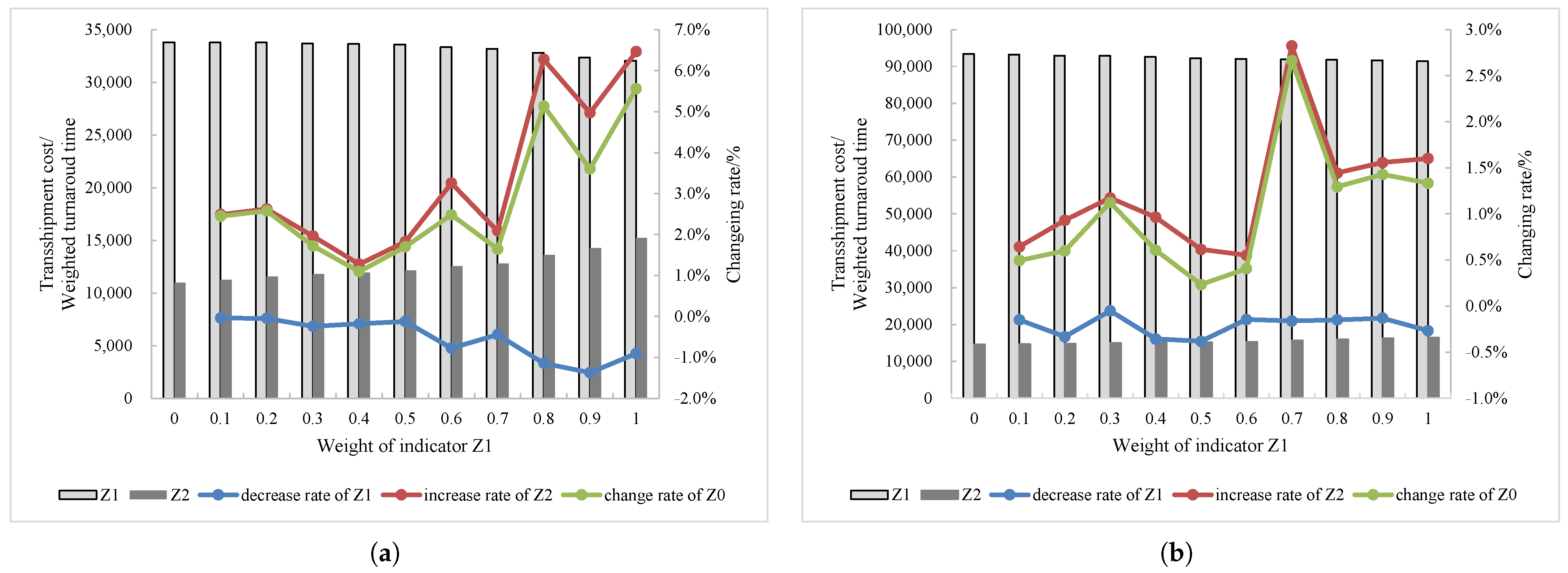
5.5.1. Sensitively Analysis for Objective Weights

The proposed model involves two key performance indicators, utilizing parameter $\lambda$ to quantify SRICT operators’ preference, where optimization results directly manifest these preference variations. For the medium-size instance I6 and large-size instance I12, we conduct comprehensive sensitivity analysis on the weight parameter. The detailed results are shown in Figure 11.

Figure 11 demonstrates that the trans-shipment cost $Z_1$ for instances I6 and I12 presents a downward trend as weight $\lambda$ increases. When weights increase from 0.8 to 0.9 and 0.4 to 0.5, the cost of instances I6 and I12 decreases most significantly, at 1.37% and 0.38%, respectively. Conversely, indicator $Z_2$ shows a positive correlation with $\lambda$. When the weight increases from 0.9 to 1 and from 0.6 to 0.7, the $Z_2$ increases by 6.46% and 2.82% for instances I6 and I12 separately. The trend of indicator $Z_2$ manifests more prominently than $Z_1$. Thus, objective $Z_0$ and indicator $Z_2$ have similar trends. Minimal growth rates occur when $\lambda$ is in the range of 0.3–0.4 for I6 and of 0.4–0.5 for I12, establishing 0.4 and 0.5 as the respective optimal weight values for these instances.

5.5.2. Sensitively Analysis for Truck Configuration

The truck undertakes horizontal transportation to connect ships, yards, and trains. Considering the busy and idle status of SRICTs and variable equipment availability, the equipment configuration is not fixed. According to industry survey, the configuration ratio between cranes and trucks usually ranges from 1:2 to 1:5. For instance, in I6, we perform sensitivity analysis on both truck number ($\left|\mathrm{\Gamma }\right|$) and configuration ratio between cranes and trucks (${\rho }_{m_v}^{nr}$ and ${\pi }_g^n$) through 64 experimental sets. The detailed results are shown in Figure 12.

(1) Trans-shipment requirements cannot be met when available trucks are less than 10, resulting in infeasible solutions, which explains the absence of corresponding results for nine-truck scenarios in Figure 12.

(2) Under the same configuration ratios, turnaround efficiency decreases with the increase in truck number. The marginal value of truck number varies with the degrees of decline. Regarding the configuration proportion between QCs and trucks, the marginal threshold stabilizes at 12 trucks for both 1:2 and 1:3 ratio, whereas it increases to 13 at 1:4 and 1:5 ratios. Regarding the configuration ratio between GCs and trucks, critical values remain constant at 12 trucks throughout operational scenarios.

(3) Under the same truck number, the weighted turnaround time decreases with the increase in configuration ratio. The threshold effect of the configuration ratio is more pronounced when total truck availability is no less than 12. Beyond this marginal value, continuing to expand the ratio has no significant improvement in accelerating the turnaround. When the total number of trucks is 10 and 11, the critical value of the configuration ratio is 1:3.

(4) Two factors have no significant impact on trans-shipment cost. Under the same configuration ratio, the operational cost generally decreases with the increase in the total number of trucks.

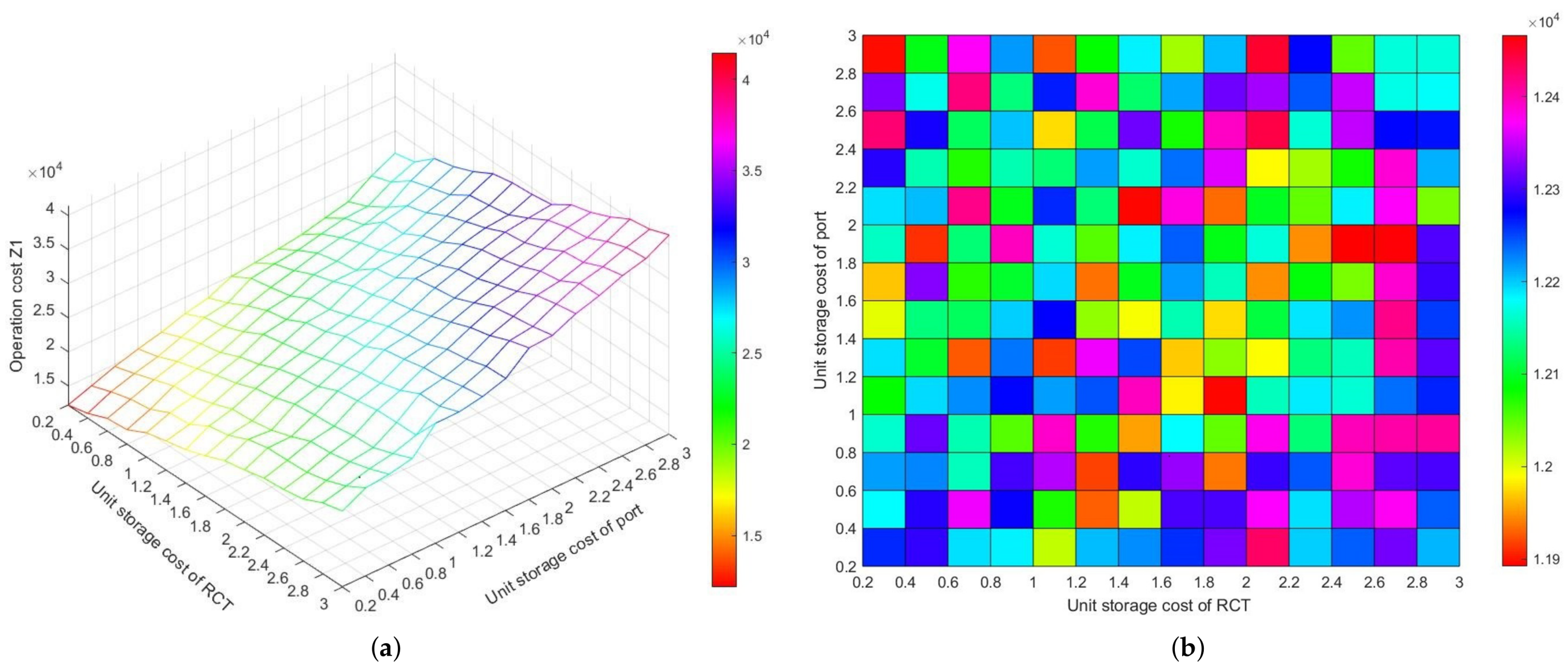
5.5.3. Sensitivity Analysis for Unit Storage Costs

Storage cost is the main component of trans-shipment costs and exerts significant influence on the yard allocation plan. Sensitivity analysis of unit storage cost is performed based on instance I6, changing parameter $c_r$ from 0.2 to 3.0 by the step of 0.2, with the results shown in Figure 13.

From Figure 13a, the trans-shipment cost exhibits a significant positive correlation with the unit storage cost. Container transfer under Mode 3 in Figure 2 requires two handling operations involving trucks, YCs, and GCs, consequently making parameter $c_1$ demonstrate a more pronounced growth trend of trans-shipment cost compared to parameter $c_2$. Moreover, a combination of unit storage costs is recommended to provide a relatively stable impact on the trans-shipment cost, such as $c_1\in [2,2.6]$ and $c_2\in [2.2,2.6]$ in instance I6. Observing Figure 13b, unit storage cost has little impact on the weighted turnaround time. Truck resources are sufficient. And objective $Z_0$ needs to balance $Z_1$ and $Z_2$. Therefore, there is no specific rule in the overall trend of indicator $Z_2$ changing unit storage cost. Nevertheless, since the unit storage cost of one yard is fixed, our approach successfully identifies the corresponding optimal unit storage cost for the counterpart yard, providing a reference for SRICT operators.

Take $c_2=2.4$ and $c_1\in [0.2,3]$ as an example,

Table 9. Container allocation scheme with a unit storage cost of ($c_1,2.4$).

${\mathit{c}}_1$	CT	M1	M2	M3	SP/(FEU·h)	SR/(FEU·h)	WTT-S/s	WTT-T/s
0.2	16	48	10	10	7177.9	3171.3	4930.6	7179.4
0.4	22	40	12	16	6927.8	3459.8	5102.3	7137.8
0.6	17	45	12	11	6743.9	3664.3	5394.3	6993.3
0.8	17	40	16	12	6405.6	3948.8	5527.5	6537.4
1	22	33	18	17	6245.1	4120.1	5692.6	12,421.8
1.2	24	35	17	16	5968.6	4409.2	5344.2	6939.8
1.4	19	34	22	12	5836.8	4516.5	5456.2	6863.7
1.6	22	35	20	13	5521.9	4829.4	5852.7	6434.7
1.8	24	29	23	16	5312.1	4993.3	6104.9	5906.7
2.0	24	26	26	16	5106.9	5125.5	6554.3	5438.4
2.2	23	29	24	15	5092.5	5178.3	6408.3	5756.8
2.4	23	26	27	15	4846.0	5557.0	6529.6	5728.1
2.6	24	24	27	17	4785.1	5474.9	6285.6	5722.7
2.8	23	25	30	13	4591.5	5645.1	6340.2	5796.9
3	27	24	27	17	4212.6	6065.8	6503.1	5622.4

shows the container allocation plan across eight key performance indices, including (1) the number of transfer batches (i.e., CT); (2) the number of arrival batches choosing Mode 1 (i.e., M1), Mode 2 (i.e., M2), and Mode 3 (i.e., M3); (3) container storage duration in port yard (i.e., SP) and RCT yard (i.e., SR); (4) WTT-S and WTT-T. From Table 9, when $c_2=2.4$, the value of indicator SR increases gradually with the increase in $c_1$, while indicator SP shows a downward trend. As a result, containers tend to store in the RCT yard, which makes the WWT-S augment gradually and the overall turnaround speed of trains accelerate.

6. Conclusions and Future Work

This study investigates container trans-shipment operations among ships, yards, and trains in SRICT systems featuring seaport–RCT separation layouts, proposing a novel joint optimization framework that simultaneously addresses yard allocation, container transfers, and truck allocation to minimize trans-shipment costs while accelerating vehicle turnaround efficiency. A two-layer APSO-GR hybrid algorithm is developed to obtain solutions. To our knowledge, the shared and joint allocation of storage yard and trucks between independently operated seaports and RCTs is investigated here for the first time. The correctness of the model and effectiveness of the algorithm are verified by comparative experiments using actual data under different solving methods, truck allocation strategies, and storage forms. Moreover, we conduct the sensitivity analysis considering objective weight, equipment configuration ratio, and unit storage cost, leading to the following key findings.

(1) The proposed APSO-GR algorithm demonstrates statistically significant superiority over CPLEX, SPSO-GR, and WPA-GR across computational efficiency, optimization accuracy, and overall search performance.

(2) Truck allocation strategy considering the freight ratio is more effective than random allocation and independent allocation strategies, particularly in enhancing vehicle turnaround efficiency with average performance improvements of 23.10% and 5.89%, respectively.

(3) Especially for SRICTs with large trans-shipment requirements, the shared yard form is more conducive due to the reasonable usage of storage space and the connection of trucks and cranes. While incurring marginally higher costs, this approach achieves a 33.45% average enhancement in handling efficiency.

(4) The multi-objective framework comprehensively considers economic and efficiency indicators while incorporating operator preferences through adjustable weighting, providing actionable decision support.

(5) Truck configuration mainly affects the turnaround of vehicles. Insufficient configuration cannot meet the trans-shipment requirements while excess capacity has no evident effect on improving turnaround efficiency but causes a waste of resources. Thus, the operators should identify the critical value.

(6) Storage costs mainly affect the trans-shipment cost. Operators decide the ratio of unit storage cost for RCT yard and port yard based on the cooperation needs by referring to our analysis results.

For future research, the cooperation and game between the port and RCT are significant referring to Jin et al. [20]. Another challenge involves enabling proactive joint optimization for bidirectional cargo flow through systematic integration of the disturbance factors of storage requirements and vehicle arrival schedule. Moreover, considering both direct and indirect trans-shipment modes, it may be interesting to study the truck scheduling optimization. Moreover, the reliance on big data and artificial intelligence algorithms like deep reinforcement learning to address resource joint allocation challenges remains an underexplored research gap.

References

1. Liu, W.Q.; Zhu, X.N.; Wang, L.; Li, S.Y. Flexible yard crane scheduling for mixed railway and road container operations in sea-rail intermodal ports with the sharing storage yard. Trans. Res. Part E-Logist. Transp. Rev. 2024, 190, 103714. [Google Scholar] [CrossRef]
2. Yan, B.C.; Jin, J.G.; Zhu, X.N.; Lee, D.H.; Wang, L.; Wang, H. Integrated planning of train schedule template and container transshipment operation in seaport railway terminals. Trans. Res. Part E-Logist. Transp. Rev. 2020, 142, 102061. [Google Scholar] [CrossRef]
3. Hu, Q.; Corman, F.; Wiegmans, B.; Lodewijks, G. A tabu search algorithm to solve the integrated planning of container on an inter-terminal network connected with a hinterland rail network. Trans. Res. Part C-Emerg. Technol. 2018, 91, 15–36. [Google Scholar] [CrossRef]
4. Guo, W.J.; Atasoy, B.; Beelaerts, W.; Negenborn, R.R. A dynamic shipment matching problem in hinterland synchromodal transportation. Decis. Support. Syst. 2020, 134, 113289. [Google Scholar] [CrossRef]
5. Feng, Y.J.; Song, D.P.; Li, D. Smart stacking for import containers using customer information at automated container terminals. Eur. J. Oper. Res. 2022, 301, 502–522. [Google Scholar] [CrossRef]
6. Lee, D.H.; Jin, J.G.; Chen, J.H. Terminal and yard allocation problem for a container transshipment hub with multiple terminals. Trans. Res. Part E-Logist. Transp. Rev. 2012, 48, 516–528. [Google Scholar] [CrossRef]
7. Zhen, L.; Wang, S.A.; Wang, K. Terminal allocation problem in a transshipment hub considering bunker consumption. Nav. Res. Logist. 2016, 63, 529–548. [Google Scholar] [CrossRef]
8. Hu, X.Y.; Liang, C.J.; Chang, D.F.; Zhang, Y. Container storage space assignment problem in two terminals with the consideration of yard sharing. Adv. Eng. Inform. 2021, 47, 101224. [Google Scholar] [CrossRef]
9. Xie, Y.; Song, D.P. Optimal planning for container prestaging, discharging, and loading processes at seaport rail terminals with uncertainty. Trans. Res. Part E-Logist. Transp. Rev. 2018, 119, 88–109. [Google Scholar] [CrossRef]
10. Carlo, H.J.; Vis, I.F.A.; Roodbergen, K.J. Storage yard operations in container terminals: Literature overview, trends, and research directions. Eur. J. Oper. Res. 2014, 235, 412–430. [Google Scholar] [CrossRef]
11. Abouelrous, A.; Dekker, R.; Bliek, L.; Zhang, Y.Q. Real-time policy for yard allocation of transshipment containers in a terminals. Transp. Res. Part B-Methodol. 2025, 192, 103138. [Google Scholar] [CrossRef]
12. Hu, H.T.; Mo, J.; Zhen, L. Integrated optimization of container allocation and yard cranes dispatched under delayed transshipment. Transp. Res. Part C-Emerg. Technol. 2024, 158, 104429. [Google Scholar] [CrossRef]
13. Wang, T.T.; Ma, H.; Xu, Z.; Xia, J. A new dynamic shape adjustment and placement algorithm for 3D yard allocation problem with time dimension. Comput. Oper. Res. 2022, 138, 105585. [Google Scholar] [CrossRef]
14. Cordeau, J.F.; Gaudioso, M.; Laporte, G.; Moccia, L. The service allocation problem at the Giola Tauro Maritime Terminal. Eur. J. Oper. Res. 2007, 176, 1167–1184. [Google Scholar] [CrossRef]
15. Cordeau, J.F.; Laporte, G.; Moccia, L.; Sorrentino, G. Optimizing yard assignment in an automotive transshipment terminal. Eur. J. Oper. Res. 2011, 215, 149–160. [Google Scholar] [CrossRef]
16. Cordeau, J.F.; Legato, P.; Mazza, R.M.; Trunfio, R. Simulation-based optimization for housekeeping in a container transshipment terminal. Comput. Oper. Res. 2015, 53, 81–95. [Google Scholar] [CrossRef]
17. Kim, K.; Jin, X.; Woo, C. A survey on sharing economy and logistics resources sharing. J. Supply Chain Manag. 2017, 17, 89–115. [Google Scholar] [CrossRef]
18. He, J.L.; Liu, Y.L.; Tan, C.M. A novel method for yard space allocation for the port with atypical container collection cycles. Adv. Eng. Inform. 2025, 64, 103040. [Google Scholar] [CrossRef]
19. Tan, C.M.; Liu, Y.L.; He, J.L.; Wang, Y.; Yu, H. Yard space allocation for container transshipment ports with mother and feeder vessels. Ocean Coast. Manag. 2024, 25, 107048. [Google Scholar] [CrossRef]
20. Jin, X.F.; Park, K.T.; Kim, K.H. Storage space sharing among container handling companies. Trans. Res. Part E-Logist. Transp. Rev. 2019, 127, 111–131. [Google Scholar] [CrossRef]
21. Karam, A.; Eltawil, A.; Harraz, N.A. Simultaneous assignment of quay cranes and internal trucks in container terminals. Int. J. Ind. Syst. Eng. 2016, 24, 107–125. [Google Scholar] [CrossRef]
22. Li, M.W.; Xu, R.Z.; Yang, Z.Y.; Hong, W.C.; An, X.G.; Yeh, Y.H. Optimization approach of berth-quay crane-truck allocation by the tide, environment and uncertainty factors based on chaos quantum adaptive seagull optimization algorithm. Appl. Soft Comput. 2024, 152, 111197. [Google Scholar] [CrossRef]
23. Zhang, X.J.; Li, H.J.; Sheu, J.B. Integrated scheduling optimization of AGV and double yard cranes in automated container terminals. Transp. Res. Part B-Methodol. 2024, 179, 102871. [Google Scholar] [CrossRef]
24. Wang, Z.X.; Chan, F.T.S.; Chung, S.H.; Niu, B. A decision support method for internal truck employment. Ind. Manag. Data Syst. 2014, 114, 1378–1395. [Google Scholar] [CrossRef]
25. Karam, A.; Eltawil, A.B. Functional integration approach for the berth allocation, and specific quay crane assignment problems. Comput. Ind. Eng. 2016, 102, 458–466. [Google Scholar] [CrossRef]
26. Chargui, K.; Zouadi, T.; EI Fallahi, A.; Reghioui, M.; Aouam, T. Berth and quay crane allocation and scheduling with worker performance variability and yard truck deployment in container terminals. Trans. Res. Part E-Logist. Transp. Rev. 2021, 154, 102449. [Google Scholar] [CrossRef]
27. Vahdani, B.; Mansour, F.; Soltani, M.; Veysmoradi, D. Bi-objective optimization for integrating quay crane and internal truck assignment with challenges of trucks sharing. Knowl. Based. Syst. 2019, 163, 675–692. [Google Scholar] [CrossRef]
28. He, J.; Zhang, W.; Huang, Y.; Yan, W. A simulation optimization method for internal trucks sharing assignment among multiple container terminals. Adv. Eng. Inform. 2013, 27, 598–614. [Google Scholar] [CrossRef]
29. Schepler, X.; Stefan, B.; Michel, S.; Sanlaville, E. Global planning in a multi-terminal and multi-modal maritime container port. Trans. Res. Part E-Logist. Transp. Rev. 2017, 100, 38–62. [Google Scholar] [CrossRef]
30. Yan, B.C.; Zhu, X.N.; Lee, D.H.; Jin, J.G.; Wang, L. Transshipment operations optimization of sea-rail intermodal container in seaport rail terminals. Comput. Ind. Eng. 2020, 141, 106296. [Google Scholar] [CrossRef]
31. Heilig, L.; Voß, S. Inter-terminal transportation: An annotated bibliography and research agenda. Flex. Serv. Manuf. J. 2016, 29, 35–63. [Google Scholar] [CrossRef]
32. Hu, Q.; Wiegmans, B.; Corman, F.; Lodewijks, G. Critical literature review into planning of inter-terminal transport: In port areas and the hinterland. J. Adv. Transp. 2019, 2019, 9893615. [Google Scholar] [CrossRef]
33. Tierney, K.; Voß, S.; Stahlbock, R. A mathematical model of inter-terminal transportation. Eur. J. Oper. Res. 2014, 235, 448–460. [Google Scholar] [CrossRef]
34. Hu, Q.; Wiegmans, B.; Corman, F.; Lodewijks, G. Integration of inter-terminal transport and hinterland rail transport. Flex. Serv. Manuf. J. 2019, 31, 807–831. [Google Scholar] [CrossRef]
35. Ramadhan, M.H.; Kamal, I.M.; Kim, D.; Bae, H. Solving the inter-terminal truck routing problem for delay minimization using simulated annealing with normalized exploration rate. J. Mar. Sci. Eng. 2023, 11, 2103. [Google Scholar] [CrossRef]
36. Fowler, R.J.; Paterson, M.S.; Tatimoto, S.L. Optimal packing and covering in the plane are NP-complete. Inf. Process. Lett. 1981, 12, 133–137. [Google Scholar] [CrossRef]
37. Tole, K.; Moqa, R.; Zheng, J.Z.; He, K. A simulated annealing approach for the circle bin packing problem with rectangular items. Comput. Ind. Eng. 2023, 176, 109004. [Google Scholar] [CrossRef]
38. Wang, X.H.; Jin, Z.H. Collaborative optimization of multi-equipment scheduling and intersection point allocation for U-shaped automated sea-rail intermodal container terminals. IEEE Trans. Autom. Sci. Eng. 2025, 22, 7373–7393. [Google Scholar] [CrossRef]
39. Xu, B.W.; Jie, D.P.; Li, J.J.; Yang, Y.S.; Wen, F.R.; Song, H.T. Integrated scheduling optimization of U-shaped automated container terminal under loading and unloading mode. Comput. Ind. Eng. 2021, 162, 107695. [Google Scholar] [CrossRef]
40. Tengecha, N.A.; Zhang, X.Y. An efficient algorithm for the berth and quay crane assignments considering operator performance in container terminal using particle swarm model. J. Mar. Sci. Eng. 2022, 10, 1232. [Google Scholar] [CrossRef]
41. Luo, Q.; Rao, Y.Q.; Peng, D. GA and GWO algorithm for the special bin packing problem encountered in field of aircraft arrangement. Appl. Soft Comput. 2022, 14, 108060. [Google Scholar] [CrossRef]
42. Vecek, N.; Crepinsek, M.; Mernik, M. On the influence of the number of algorithms, problems, and independent runs in the comparison of evolutionary algorithms. Appl. Soft Comput. 2017, 54, 23–45. [Google Scholar] [CrossRef]
43. Wieckowski, J.; Salabun, W. Sensitivity analysis approaches in multi-criteria decision analysis: A systematic review. Appl. Soft Comput. 2023, 148, 110915. [Google Scholar] [CrossRef]
Figure 1. Separation layout of SRICTs and transshipment flow for import container.
Jmse 13 00983 g001
Figure 2. Trans-shipment modes of import sea–rail multimodal container.
Jmse 13 00983 g002
Figure 3. Twelve states of import trans-shipment containers.
Jmse 13 00983 g003
Figure 4. Overall framework of the APSO-GR algorithm.
Jmse 13 00983 g004
Figure 5. Procedural workflow of the APSO-GR algorithm.
Jmse 13 00983 g005
Figure 6. Encoding and decoding samples of one batch.
Jmse 13 00983 g006
Figure 7. A sample for truck allocation strategy for vehicles.
Jmse 13 00983 g007
Figure 8. Remaining capacity of trucks required by ships.
Jmse 13 00983 g008
Figure 9. Yard allocation and truck allocation plans of instance I6: (a) Yard allocation plan. (b) Truck allocation plan.
Jmse 13 00983 g009
Figure 10. Comparative results of shared yard form and traditional form: (a) The weighted turnaround time. (b) The value of indicators and gaps.
Jmse 13 00983 g010
Figure 11. Results of two instances for different indicator weights: (a) Results of instance I6. (b) Results of instance I12.
Jmse 13 00983 g011
Figure 12. Results for truck number and the configuration ratio between cranes and trucks: (a) Configuration between QCs and trucks. (b) Configuration between GCs and trucks.
Jmse 13 00983 g012
Figure 13. Results varied with unit storage cost: (a) Trans-shipment costs. (b) Weighted turnaround time.
Jmse 13 00983 g013