An Adaptive Neural Network Fuzzy Sliding Mode Controller for Tracking Control of Deep-Sea Mining Vehicles

Abstract

Traditional track-driven deep-sea nodule mining solutions significantly disrupt seabed ecosystems, making them unsuitable for commercial application. In contrast, ROV-like alternatives, such as the hovering mining vehicle, or HMV, offer substantial improvement in this regard and are deemed to be a viable way forward. This paper proposes an adaptive neural network fuzzy sliding mode controller architecture for the underwater trajectory tracking of HMV. The algorithm, named the Adaptive Radial Basis Function Neural Network Fuzzy Sliding Mode Controller (ARFSMC), replaces modeled vehicle dynamics with a radial basis function neural network (RBFNN). To enhance disturbance rejection, an adaptive mechanism is applied to the RBFNN output weighting matrix. Additionally, a fuzzy inference system (FIS) is implemented as the switching term, replacing the traditional signum function, to reduce high-frequency oscillations in the control signal. The stability of the algorithm under unknown external disturbance was confirmed via Lyapunov stability analysis. To validate the ARFSMC’s performance, three numerical simulation cases were conducted, each designed to reflect an expected operation scenario of the HMV, through which the tracking performance of the ARFSMC under time-varying system inertia is validated and benchmarked against conventional sliding mode control (CSMC) and double-loop sliding mode control (DSMC). The simulation results confirm that comparing the above two controllers, the root mean square error (RMSE) of the ARFSMC is reduced by 15.0% and 11.4%, respectively. And when comparing the CSMC, the chattering is reduced by 97.8%. Both indicate their high robustness and superior performance in tracking control. The controller development and numerical validation in this work are aimed at the trajectory tracking challenge of the HMV in deep-sea mining operation. The dynamical modeling of the vehicle is based on parameters of the HaiMa ROV. External disturbance from currents were considered as sinusoidal functions modified with random noise.

1. Introduction

The global ocean contains a vast amount of high-value mineral deposits, many found on the deep-sea floor as scattered polymetallic nodule fields, crucial resources to decarbonize the current economy [1]. Classical deep-sea nodule mining solutions are of the ship–pipe–buffer–link–miner configuration, in which a track-driven collector rover on the seabed extracts the mineral nodules that are then sent to surface storage by hydrotransport [2]. However, this type of mining operation would induce large disturbance to seabed ecosystems and is currently under heavy scrutiny from the International Sea Authority (ISA) [3,4]. To mitigate the impact of deep-sea nodule mining on the seafloor, buoyancy-based ROV-type collector designs, addressed as the hovering mining vehicle (HMV) in this paper, have emerged as a possible alternative for track-driven miners, as shown in Figure 1 [5]. One key challenge associated with the HMV is its trajectory tracking, as a buoyancy-based collector has increased dimensions of motion compared to a tracked rover and is more susceptible to external time-varying disturbances from currents and seafloor terrain. Furthermore, the underwater dynamical characteristics of the HMV are highly nonlinear and strongly coupled, often times difficult to model accurately beforehand. Therefore, high-precision trajectory tracking of the HMV collector is key to unlocking increasingly environmentally friendly deep-sea nodule mining solutions.

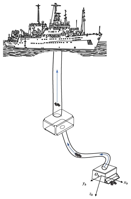
Figure 1. HMV concept.

Because the dynamical behavior of underwater vehicles is in general highly nonlinear in nature, controller algorithms whose effective implementation does not rely on knowledge of the plant dynamics, such as the proportional–integral–derivative (PID) controller and the fuzzy logic controller (FLC), are widely adopted in the field of underwater robotics. The FLC employs a predefined expertise rule base to map system states to control input, while PID is a popular classical linear controller that has the merit of simplicity. Recent increases in hardware computational power have seen artificial neural networks (ANNs) built into a classical PID closed loop to update PID gains online in an effort to form an adaptive PID algorithm that promises better performance and robustness controlling nonlinear and time-varying systems, demonstrating the potential of machine learning in enhancing controller performance [6]. Apart from these, (plant) model-based controllers, for example, the sliding mode controller (SMC), are also popular. The SMC works by using a switching function to switch between two control laws so that an appropriate control signal can be generated to first pull the errors toward a user-specified sliding surface, essentially a lower-order function that is a ‘slice’ of the original error dynamics phase portrait (switching control law); once on the sliding surface, the dynamics are dependent on the design of the surface and the errors are slid on the sliding surface to eventually converge to the zero vector (the equivalent control law). The SMC offers excellent robustness against system uncertainties and external disturbances, as these can be overcome by setting large enough gains in the switching function. However, due to the discontinuous nature of the switching term, the implementation of the SMC on discrete time systems can cause a phenomenon known as chattering—high-frequency limit cycle oscillations about the sliding surface, particularly obvious under high switching gains, reducing the lifespan of actuators (e.g., motors on an ROV) and potentially exciting unmodeled high-frequency modes in doing so [7,8]. Work on the classic SMC to enhance its robustness and mitigate against the chattering problem has been a continuous effort over the years, which saw developments of different disturbance compensation schemes [9,10], the adoption of the boundary layer in proximity to the sliding surface where gains may be tuned down proportionally to distance from the sliding surface (saturation) [11], as well as different continuous switching function designs to replace the classically used signum function based ones [12].

Advances in modern control theory are leading to a popular rise in a mixed control strategy for underwater robotics. Bessa et al. [9], on the basis of the conventional SMC structure, introduced a fuzzy logic inference scheme for the online estimation of disturbances using sliding surface parameters, and together with a boundary layer saturation design, the adaptive fuzzy logic sliding mode controller (AFSMC) achieved robust depth control of an ROV. Wang et al. [13] employed the radial basis function neural network (RBFNN) to perform an online approximation of the general uncertainty, and then, in combination with the SMC, achieved fault-tolerant control (FTC) of an ROV, with numerical simulations performed on a 4-DOF ROV model showing a superior performance compared with traditional fault detection and diagnosis (FDD) unit-informed FTC in the case of thruster failure. A double-loop sliding mode controller (DSMC) divides the problem of trajectory tracking into position tracking (kinematic control) and velocity tracking (dynamic control). Qiao et al. [14] and Li et al. [15] proposed a DSMC architecture based on integral terminal sliding mode control (ITSMC) or fast terminal integral sliding mode control (FITSMC), and implemented an adaptive mechanism to provide an online estimation of general uncertainty; the numerical simulation showed that the method successfully enforced finite-time convergence of the ROV position and velocity tracking errors to zero under modulated time-varying disturbances. Based on an integral DSMC, Huang et al. [16] adopted the inverse tangent function in place of conventional signum function as the switching term to achieve precision trajectory tracking of work-class ROV. Xia et al. [17] designed an adaptive back-stepping terminal SMC scheme with integrated ANN and disturbance observer for uncertainty estimation. Yang et al. [18] employed an offline trained recurrent neural network (RNN) model to estimate and compensate for uncertainty and a fuzzy-logic-based switching term to suppress chattering. Wang et al. [19] developed an adaptive anti-disturbance SMC for ROV usage, adopting saturation to reduce chattering.

Inspired by existing ROV trajectory tracking solutions, this paper presents an adaptive SMC algorithm for the trajectory tracking problem of the HMV. A radial basis function neural network (RBFNN) model with an adaptive output weighting matrix is deployed to identify and compensate for system uncertainty and external disturbances. To reduce chattering, a fuzzy inference system (FIS) is constructed for use as the SMC switching term.

2. HMV Modeling

2.1. Kinematics

To model the motion of the HMV, like it is for any underwater vehicle, it is convenient to define two reference frames: an inertial reference frame and a body-fixed reference frame. The origin of the body-fixed frame is set to the HMV’s center of mass, while the origin of the inertial frame is a fixed point on the ground. An illustration is presented in Figure 2.

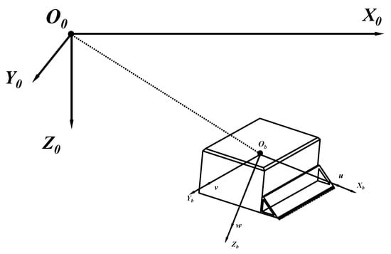
Figure 2. Reference frames.

The HMV has six degrees of freedom (DOF). Its position vector, measured with respect to the inertial reference frame, is denoted $\mathit{\eta }={[x,y,z,\varphi ,\theta ,\psi ]}^T$. The velocity vector of the HMV, measured with respect to the body-fixed frame, is denoted $\mathit{\nu }={[u,v,w,p,q,r]}^T$. The first three elements in the two vectors represent linear displacements and linear velocities, while the last three elements are attitude angles and angular velocities of the HMV, in respective coordinate frames. For an ROV, the metacentric height is typically large enough to self-stabilize in the roll and pitch degrees of freedom, and since practical trajectory tracking of the HMV would be primarily associated with the surge, sway, heave, and yaw degrees of freedom, the kinematic model is simplified to four DOF. The vectors, thereby, are reduced to $\mathit{\eta }={[x,y,z,\psi ]}^T$ and $\mathit{\nu }={[u,v,w,r]}^T$. The relationship between $\mathit{\eta }$ and $\mathit{\nu }$ is described by the transformation:

$$\begin{array}{c}\hfill \dot{\mathit{\eta }}=\mathbf{J}\left(\mathit{\eta }\right)\mathit{\nu }\end{array}$$

(1)

where $\mathbf{J}\left(\mathit{\eta }\right)$ is the Jacobian matrix. Writing Equation (1) in matrix–vector form gives

$$\begin{array}{c}\hfill \left[\begin{array}{c}\dot{x}\\ \dot{y}\\ \dot{z}\\ \dot{\psi }\end{array}\right]=\left[\begin{array}{cccc}cos\psi & -sin\psi & 0& 0\\ sin\psi & cos\psi & 0& 0\\ 0& 0& 1& 0\\ 0& 0& 0& 1\end{array}\right]\left[\begin{array}{c}u\\ v\\ w\\ r\end{array}\right]\end{array}$$

(2)

2.2. Dynamics

Following the general ROV modeling approach, the dynamics of the HMV are governed by [20]

$$\begin{array}{c}\hfill \mathbf{M}\dot{\mathit{\nu }}+\mathbf{C}\left(\mathit{\nu }\right)\mathit{\nu }+\mathbf{D}\left(\mathit{\nu }\right)\mathit{\nu }+\mathbf{g}\left(\mathit{\eta }\right)=\mathit{\tau }+{\mathit{\tau }}_{\mathbf{d}}\end{array}$$

(3)

where $\mathbf{M}\in {\mathbb{R}}^{4\times 4}$ describes the vehicle inertia, $\mathbf{C}\in {\mathbb{R}}^{4\times 4}$ is the Coriolis and centripetal forcing matrix, $\mathbf{D}\in {\mathbb{R}}^{4\times 4}$ is the hydrodynamic damping matrix, $\mathbf{g}\in {\mathbb{R}}^{4\times 1}$ is the combined vehicle weight and buoyancy forcing, $\mathit{\tau }\in {\mathbb{R}}^{4\times 1}$ is the control forcing and moments, and ${\mathit{\tau }}_{\mathit{d}}\in {\mathbb{R}}^{4\times 1}$ contains disturbances. The matrix $\mathbf{M}$, $\mathbf{C}$, $\mathbf{D}$, and the vector $\mathbf{g}$ are given by

$$\begin{array}{c}\hfill \mathbf{M}=diag\left\{\begin{array}{c}m-X_{\dot{u}},m-Y_{\dot{v}},m-Z_{\dot{w}},I_z-N_{\dot{r}}\end{array}\right\}\end{array}$$

(4)

$$\begin{array}{c}\hfill \mathbf{C}\left(\mathit{\nu }\right)=\left[\begin{array}{cccc}0& 0& 0& -\left(\begin{array}{c}m-Y_{\dot{v}}\end{array}\right)v\\ 0& 0& 0& \left(\begin{array}{c}m-X_{\dot{u}}\end{array}\right)u\\ 0& 0& 0& 0\\ \left(\begin{array}{c}m-Y_{\dot{v}}\end{array}\right)v& -\left(\begin{array}{c}m-X_{\dot{u}}\end{array}\right)u& 0& 0\end{array}\right]\end{array}$$

(5)

$$\begin{array}{c}\hfill \mathbf{D}=diag\left\{\begin{array}{c}{X}_u+X_{u\left|u\right|}\left|u\right|,Y_v+Y_{v\left|v\right|}\left|v\right|,Z_w+Z_{w\left|w\right|}\left|w\right|,N_r+N_{r\left|r\right|}\left|r\right|\end{array}\right\}\end{array}$$

(6)

$$\begin{array}{c}\hfill \mathbf{G}=\left[\begin{array}{c}0\\ 0\\ W-B\\ 0\end{array}\right]\end{array}$$

(7)

where m is the mass of the HMV, $I_z$ is the moment of inertia about the HMV body-fixed z-axis, $X_{\dot{u}}{Y}_{\dot{v}}{Z}_{\dot{w}}$ are additional masses on the vehicle, $N_{\dot{r}}$ is an additional moment of inertia, $X_u{X}_{u\left|u\right|}{Y}_v{Y}_{v\left|v\right|}{Z}_w{Z}_{w\left|w\right|}{N}_r{N}_{r\left|r\right|}$ are hydrodynamic coefficients, and W and B are weight and buoyancy, respectively.

Using the transformation described in Equation (2), the dynamic equations of motion of the HMV in the inertial reference frame are

$$\begin{array}{c}\hfill {\mathbf{M}}_{\mathit{\eta }}\left(\mathit{\eta }\right)\ddot{\mathit{\eta }}+{\mathbf{C}}_{\mathit{\eta }}(\mathit{\nu },\mathit{\eta })\dot{\mathit{\eta }}+{\mathbf{D}}_{\mathit{\eta }}(\mathit{\nu },\mathit{\eta })+{\mathbf{g}}_{\mathit{\eta }}\left(\mathit{\eta }\right)={\mathit{\tau }}_{\mathit{\eta }}+{\mathit{\tau }}_{\mathbf{d}}\end{array}$$

(8)

where the subscript $\mathit{\eta }$ indicates inertial frame values. Specifically,

$$\begin{array}{cc}\hfill & {\mathbf{M}}_{\mathit{\eta }}\left(\mathit{\eta }\right)={\mathbf{J}}^{-T}\mathbf{M}{\mathbf{J}}^{-1}\hfill \end{array}$$

(9)

$$\begin{array}{cc}\hfill & {\mathbf{C}}_{\mathit{\eta }}(\mathit{\nu },\mathit{\eta })={\mathbf{J}}^{-T}\left[\begin{array}{c}\mathbf{C}\left(\mathit{\nu }\right)-\mathbf{M}{\mathbf{J}}^{-1}\dot{\mathbf{J}}\end{array}\right]{\mathbf{J}}^{-1}\hfill \end{array}$$

(10)

$$\begin{array}{cc}\hfill & {\mathbf{D}}_{\mathit{\eta }}(\mathit{\nu },\mathit{\eta })={\mathbf{J}}^{-T}\mathbf{D}\left(\mathit{\nu }\right){\mathbf{J}}^{-1}\hfill \end{array}$$

(11)

$$\begin{array}{cc}\hfill & {\mathbf{g}}_{\mathit{\eta }}\left(\mathit{\eta }\right)={\mathbf{J}}^{-T}\mathit{\tau }\hfill \end{array}$$

(12)

$$\begin{array}{cc}\hfill & {\mathit{\tau }}_{\mathit{d}}={\mathbf{J}}^{-T}{\mathit{\tau }}_{\mathit{d}}\hfill \end{array}$$

(13)

3. Controller Design

3.1. Conventional Sliding Mode Controller (CSMC)

The trajectory tracking error is defined as

$$\begin{array}{c}\hfill \mathbf{e}={\mathit{\eta }}_{\mathit{d}}-\mathit{\eta }\end{array}$$

(14)

where ${\mathit{\eta }}_{\mathit{d}}$ is the desired position for the vehicle. The sliding surface is defined by the expression $\mathbf{s}(\mathbf{e},\dot{\mathbf{e}})=\mathbf{0}$, where $\mathbf{s}\in {\mathbb{R}}^{4\times 1}$ is known as the switching function. In CSMC, the switching function is typically constructed as a linear combination of the error vector and its time derivative in the following way:

$$\begin{array}{c}\hfill \mathbf{s}=\mathit{\lambda }\mathbf{e}+\dot{\mathbf{e}}\end{array}$$

(15)

Differentiating Equation (15) with respect to time gives

$$\begin{array}{c}\hfill \dot{\mathbf{s}}=\mathit{\lambda }\dot{\mathbf{e}}+\ddot{\mathbf{e}}\end{array}$$

(16)

The total control action outputted by the CSMC, $\mathit{\tau }$, consists of the equivalent control component ${\mathit{\tau }}_{\mathit{eq}}$ and the switching control component ${\mathit{\tau }}_{\mathit{sw}}$, as described by Equation (17). When the error states ${[\mathbf{e},\dot{\mathbf{e}}]}^T$ are away from the defined sliding surface, the switching control ${\mathit{\tau }}_{\mathit{sw}}$ dominates to drive the system toward the sliding surface; once the error states are on the sliding surface ($\mathbf{s}=\mathbf{0}$), the equivalent control ${\mathit{\tau }}_{\mathit{eq}}$ enforces the reduced-order dynamics $\dot{\mathbf{e}}=-\mathit{\lambda }\mathbf{e}$, which drives the error states to asymptotically converge toward the zero vector:

$$\begin{array}{c}\hfill \mathit{\tau }={\mathit{\tau }}_{\mathit{eq}}+{\mathit{\tau }}_{\mathit{sw}}\end{array}$$

(17)

The core of the SMC is the switching term. Here, the traditionally used signum function is adopted as the switching term. The signum function is defined as, for some independent variable x,

$$\begin{array}{c}\hfill \mathbf{sgn}\left(x\right)=\left\{\begin{array}{cc}-1\hfill & \mathrm{if}x<0\hfill \\ 0\hfill & \mathrm{if}x=0\hfill \\ 1\hfill & \mathrm{if}x>0\hfill \end{array}\right.\end{array}$$

(18)

To achieve sliding mode control, $\dot{\mathbf{s}}$ must be of the opposite sign to $\mathbf{s}$ when $\mathbf{s}\ne \mathbf{0}$, and zero when $\mathbf{s}=\mathbf{0}$. For this reason, a device known as the reaching law is used to output the appropriate $\dot{\mathbf{s}}$ given $\mathbf{s}$. In this work, the exponential reaching law $\dot{\mathbf{s}}=-k\mathbf{s}-\sigma \mathbf{sgn}\left(\mathbf{s}\right)$ is adopted. Combining this and Equations (8), (14) and (16), we arrive at the control law of the CSMC:

$$\begin{array}{c}\hfill \mathit{\tau }={\mathbf{C}}_{\mathit{\eta }}\dot{\mathit{\eta }}+{\mathbf{D}}_{\mathit{\eta }}\dot{\mathit{\eta }}+{\mathbf{g}}_{\mathit{\eta }}+{\mathbf{M}}_{\mathit{\eta }}(\mathit{\lambda }\dot{\mathbf{e}}+{\ddot{\mathit{\eta }}}_{\mathbf{d}}+k\mathbf{s}+\mathit{\sigma }\mathbf{sgn}\left(\mathbf{s}\right))\end{array}$$

(19)

where $\mathit{\sigma }$ is some constant gain. This CSMC is capable of handling basic vehicle position control; however, due to the discontinuous switching term choice, significant chattering is very likely to be present in the control signal from this controller. Moreover, the HMV can be expected to receive unknown external disturbances, possibly time-varying, from its complex deep-sea operation environment. Thus, the CSMC will not suffice for operational trajectory tracking of the HMV. Section 3.2 of this paper thereby presents an improved control scheme which, on the basis of the CSMC, deploys an ANN and FIS to alleviate said issues.

3.2. Adaptive Radial Basis Function Neural Network Fuzzy Logic Controller (ARFSMC)

3.2.1. RBF Neural Network

In recent times, ANN models have found wide use in the trajectory tracking of unmanned underwater vehicles (UUVs) [21,22,23,24]. The radial basis function neural network (RBFNN) is a class of ANN that uses radial basis functions (RBFs) as the activation function. Characterized by its relatively simple structure and strong local approximation capability, the RBFNN is a popular solution for uncertainty compensation on UUVs. In the ARFSMC, output from an offline trained RBFNN model replaces the model-based terms of ${\mathit{\tau }}_{\mathit{eq}}$ in the CSMC control law, ${\mathbf{C}}_{\mathit{\eta }}\dot{\mathit{\eta }}+{\mathbf{D}}_{\mathit{\eta }}\dot{\mathit{\eta }}+{\mathbf{g}}_{\mathit{\eta }}$. The RBFNN consists of three feedforward layers: an input layer, a hidden layer, and an output layer. The input layer accepts input data and passes them to the hidden layer, where at each hidden layer node (neuron), the nodal RBF activation function maps the input data vector into a firing strength value of the particular node, and finally, outputs are produced as linear combinations of the hidden layer firing strength values. The RBFNN model in this work contains five hidden layer nodes and employs the Gaussian RBF defined in Equation (20) as the activation function:

$$\begin{array}{c}\hfill h_j=exp(-{\displaystyle \frac{\parallel \mathbf{s}-{\mathbf{c}}_j{\parallel }^2}{2{b_j}^2}}),j=1,2,\dots ,5\end{array}$$

(20)

where j denotes a specific hidden layer node; $\mathbf{s}\in {\mathbb{R}}^{4\times 1}$ is the SMC switching function value, itself input to the RBFNN model; $b_j\in \mathbb{R}$ and ${\mathbf{c}}_j\in {\mathbb{R}}^{4\times 1}$ are tunable parameters; ${\mathbf{c}}_j$ governs the center position of the nodal activation function in input space; and $b_j$ controls the variance of the function.

The output of the RBFNN is a linear combination of nodal firing strengths, as shown in Equation (21):

$$\begin{array}{c}\hfill \widehat{\mathit{f}}={\widehat{\mathbf{W}}}^{\mathbf{T}}\mathit{h}\end{array}$$

(21)

where ${\widehat{\mathbf{W}}}^{\mathbf{T}}\in {\mathbb{R}}^{4\times 5}$ is the output weighting matrix. ${\widehat{\mathbf{W}}}^{\mathbf{T}}$ describes the linear relationship between the hidden layer firing strengths $\mathit{h}\in {\mathbb{R}}^{5\times 1}$ and the target output vector $\widehat{\mathit{f}}\in {\mathbb{R}}^{4\times 1}$. The initial weightings ${\widehat{\mathbf{W}}}^{\mathbf{T}}$ are small quantities; the RBF center position parameters are $\mathit{c}={[-1,-0.5,0,0.5,1]}^T$, variance parameter $\mathit{b}={[3,3,3,3,3]}^T$. Finally, let

$$\begin{array}{c}\hfill \widehat{\mathit{f}}={\widehat{\mathit{\tau }}}_{\mathit{eq}}\end{array}$$

(22)

where ${\widehat{\mathit{\tau }}}_{\mathit{eq}}$ is to replace the conventionally model-based terms in the SMC equivalent control component ${\mathit{\tau }}_{\mathit{eq}}$, i.e., ${\mathbf{C}}_{\mathit{\eta }}\dot{\mathit{\eta }}+{\mathbf{D}}_{\mathit{\eta }}\dot{\mathit{\eta }}+{\mathbf{g}}_{\mathit{\eta }}$ in Equation (19).

3.2.2. Fuzzy Inference System

The switching term is key to the desirable robustness of an SMC, but in the CSMC, due to the discontinuous nature of the signum function, it also induces chattering [25]. The ARFSMC adopts a Mamdani method FIS in place of the constant switching term gain $\mathit{\sigma }$ in the CSMC, and this modifies the switching control component into a smooth function. The FIS comprises a fuzzifier, a fuzzy rule base, a fuzzy inference engine, and a defuzzifier. The fuzzifier maps a crisp input to the input fuzzy set based on the degrees of the input membership functions. The fuzzy rule base is a collection of fuzzy rules formulated based on human expertise on the problem. In accordance with the fuzzy rules, the fuzzy inference engine maps the input fuzzy set for the particular crisp input to respective firing strengths of the fuzzy rules via the output membership functions; then, the engine composes an output fuzzy set based on the firing strengths. Finally, the defuzzifier maps the output fuzzy set to a crisp output. The inputs to the FIS are entries of the switching function, $s_i\in \mathbf{s},i=1,2,3,4$. The outputs of the FIS are entries of the CSMC constant switching term gain replacement, ${\mu }_i\in \widehat{\mathit{\mu }},i=1,2,3,4$. Correspondingly, the input and output fuzzy sets are defined as

$$\begin{array}{c}\hfill A=\left\{\begin{array}{c}N,Z,P\end{array}\right\}W=\left\{\begin{array}{c}N,Z,P\end{array}\right\}\end{array}$$

(23)

The membership functions associated with the sets are presented in Appendix A. The fuzzy rules are stated in the IF–THEN form, as shown in Equation (24), where $r=1,2,3$ indicates members of the relevant sets. The $\mathbf{IF}$ part of the rule statement is referred to as the antecedent, while the $\mathbf{THEN}$ part is known as the consequent. In order to realize the fuzzification of the switching control term, only the equivalent control is retained in the absence of disturbances. The specific fuzzy rule definitions are presented in Appendix A:

$$\begin{array}{c}\hfill {\mathbf{R}}^{\mathbf{r}}:\mathbf{IF}{s}_i\mathbf{is}{A}^r,\mathbf{THEN}{\mu }_i\mathbf{is}{W}^r\end{array}$$

(24)

It should be noted in this FIS that each fuzzy rule maps a unique input membership function value to an output membership function value (i.e., $A^r\to W^r$); therefore, the r-th fuzzy output set member has the same value as the firing strength of the r-th fuzzy rule, which has the same value as the evaluation of the r-th output membership function. Because in each of the three fuzzy rules, the antecedent only concerns one input fuzzy set member, there is no need to perform any logical operation.

The center-of-gravity (CoG) method is used for defuzzification, which defines the crisp output as the centroid location of the output fuzzy set, as shown in Equation (25), where ${\mu }_i$ is an entry of the FIS output vector $\widehat{\mathit{\mu }}\in {\mathbb{R}}^{4\times 1}$, and ${\mu }_{A^r}$ is the firing strength of the r-th fuzzy rule; both are functions of $s_i$. $z_r$ is the centroid location of the r-th member of the output fuzzy set in crisp output space:

$$\begin{array}{cc}\hfill {\mu }_i\left(s_i\right)& ={\displaystyle \frac{{\displaystyle \sum _{r=1}^3}({\mu }_{A^r}\left(s_i\right)·z_r)}{{\displaystyle \sum _{r=1}^3}{\mu }_{A^r}\left(s_i\right)}}\hfill \end{array}$$

(25)

$$\begin{array}{cc}\hfill & =\mathit{\xi }{\left(s_i\right)}^T\mathbf{z}\hfill \end{array}$$

(26)

Alternatively, Equation (25) can be rewritten into Equation (26), where $\mathbf{z}={[z_1,z_2,z_3]}^T$ and $\mathit{\xi }\left(s_i\right)={[{\xi }_1\left(s_i\right),{\xi }_2\left(s_i\right),{\xi }_3\left(s_i\right)]}^T\in {\mathbb{R}}^{3\times 1}$ is the normalized rule firing strengths vector, whose entry ${\xi }_r\left(s_i\right)$ is

$$\begin{array}{c}\hfill {\xi }_r\left(s_i\right)={\displaystyle \frac{{\mu }_{A^r}\left(s_i\right)}{{\displaystyle \sum _{r=1}^3}{\mu }_{A^r}\left(s_i\right)}}\end{array}$$

(27)

Finally, let the FIS output be the ARFSMC switching term gain:

$$\begin{array}{c}\hfill \widehat{\mathit{\mu }}=\widehat{\mathit{\sigma }}\end{array}$$

(28)

where $\widehat{\mathit{\sigma }}$ is to replace the constant gain $\mathit{\sigma }$ in Equation (19). In summary, the input variable to the FIS is the sliding function $\mathit{s}$. The value of $\mathit{s}$ reflects the deviation in error states from the sliding surface. The input space is $\mathit{s}\in [-1,1]$, as this mostly covers the normal operation of the HMV. Three linguistic descriptors $\mathit{N}$ (Negative), $\mathit{Z}$ (zero), $\mathit{P}$ (Positive) are used to construct the membership functions. The input membership functions are classical triangular and trapezoidal functions to ensure computational efficiency and smoothness. The FIS output variable $\mathit{\mu }$ is used as a smooth replacement for the conventional discontinuous sign function switching term found in the CSMC. The output space also ranges $[-1,1]$ as to fit with the working of the SMC switching term.

3.3. Stability Analysis

Replacing $\mathit{\sigma }$ and ${\mathbf{C}}_{\mathit{\eta }}\dot{\mathit{\eta }}+{\mathbf{D}}_{\mathit{\eta }}\dot{\mathit{\eta }}+{\mathbf{g}}_{\mathit{\eta }}$ in Equation (19) with $\widehat{\mathit{\sigma }}$ and ${\mathit{\tau }}_{\mathit{eq}}$, we arrive at the control law of the ARFSMC, as shown in Equation (29):

$$\begin{array}{c}\hfill \mathit{\tau }=\widehat{\mathit{f}}+{\mathbf{M}}_{\mathit{\eta }}(\mathit{\lambda }\dot{\mathbf{e}}+{\ddot{\mathit{\eta }}}_{\mathit{d}}+k\mathbf{s}+\widehat{\mu }\mathbf{sgn}\left(\mathbf{s}\right))\end{array}$$

(29)

The final controller architecture is shown in Figure 3. Recall that there are three customizable variables in the RBFNN model: $\widehat{\mathbf{W}}$, ${\mathbf{c}}_j$, and $b_j$; among them, the output weighting matrix $\widehat{\mathbf{W}}$ has the most significant impact on the tracking performance. To further increase the robustness of the ARFSMC while retaining simplicity, it is decided that an adaptive mechanism will be applied on $\widehat{\mathbf{W}}$ to compensate for the uncertainty within it. The rest of this section describes the insertion of the adaptive mechanism based on Lyapunov stability analysis.

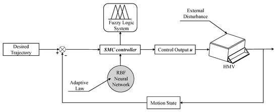
Figure 3. The ARFSMC architecture.

The Lyapunov function candidate is defined as follows:

$$\begin{array}{c}\hfill \mathbf{V}={\displaystyle \frac{1}{2}}{\mathbf{s}}^T\mathbf{s}+{\displaystyle \frac{1}{2}}{\tilde{\mathbf{W}}}^T{\mathbf{\Gamma }}^{-1}\tilde{\mathbf{W}}\end{array}$$

(30)

where $\tilde{\mathbf{W}}$ is the uncertainty in the RBFNN output weighting matrix, $\tilde{\mathbf{W}}={\mathbf{W}}^{*}-\widehat{\mathbf{W}}$, with ${\mathbf{W}}^{*}$ being some optimal RBFNN output weighting matrix. $\mathbf{\Gamma }$ is a matrix of constant gains.

Differentiating Equation (30) with respect to time yields

$$\begin{array}{c}\hfill \dot{\mathbf{V}}={\mathbf{s}}^T\dot{\mathbf{s}}+{\tilde{\mathbf{W}}}^T{\mathbf{\Gamma }}^{-1}\dot{\tilde{\mathbf{W}}}\end{array}$$

(31)

There exists an error $ϵ$ in the output of the RBFNN. For a generic input $\mathbf{x}$, the true value of what the network is tasked with approximating can be expressed as

$$\begin{array}{c}\hfill \mathit{f}\left(\mathbf{x}\right)={\tilde{\mathbf{W}}}^T\mathit{h}+\mathit{ϵ}\end{array}$$

(32)

Combining Equations (31) and (32),

$$\begin{array}{c}\hfill \dot{\mathbf{V}}=-{\mathbf{s}}^T\widehat{\mathit{\mu }}\left(\mathbf{s}\right)\mathbf{sgn}\left(\mathbf{s}\right)-{\mathbf{s}}^T\mathit{ϵ}-{\mathbf{s}}^T\mathbf{d}\left(t\right)+{\tilde{\mathbf{W}}}^T{\mathbf{\Gamma }}^{-1}\dot{\tilde{\mathbf{W}}}\end{array}$$

(33)

where $\mathbf{d}\left(t\right)$ represents unknown disturbances in the system.

The adaptive mechanism is designed as

$$\begin{array}{c}\hfill \dot{\widehat{\mathbf{W}}}=\mathbf{\Gamma }\mathit{h}{\mathbf{s}}^T\end{array}$$

(34)

Substituting Equation (34) into Equation (33), and making the following assumptions:

Assumption 1.

The disturbances $\mathbf{d}\left(t\right)$ and RBFNN approximation error ϵ are bounded from above, meaning $\mathbf{d}\left(t\right)\le \mathbf{D},\mathit{ϵ}\le {\mathit{ϵ}}_b$, where $\mathbf{D}$ and ${\mathit{ϵ}}_b$ are upper bounds of $\mathbf{d}\left(t\right)$ and ϵ.

Assumption 2.

The output of the FIS $\widehat{\mathit{\mu }}\left(\mathbf{s}\right)$ is bounded from below.

Then

$$\begin{array}{c}\hfill \dot{\mathbf{V}}\le -k{\parallel \mathbf{s}\parallel }^2-\widehat{\mathit{\mu }}\left(\mathbf{s}\right)+\mathit{\delta }\le 0\end{array}$$

(35)

where $\mathit{\delta }$ is a small redundancy term. Therefore, from Lyapunov stability theory, the system is asymptotically stable, and convergence of the error states to the sliding surface is guaranteed.

4. Numerical Validation

To further validate the effectiveness of the ARFSMC in tracking the HMV trajectory, numerical simulations are performed based on three expected operational scenarios: (A) vertical deployment in the mining zone, (B) linear translation motion of the vehicle with time-varying mass, and (C) spiral motion. In all three cases, hydrodynamic coefficients of the HMV are approximated by those of the HaiMa ROV. Lumped external disturbance and model uncertainty are modulated as $d_i=0.1M_{ii}sin\left(0.1t\right)+5\mathrm{rand}\left(1\right),i=1,2,3,4$, where $M_{ii}$ is a diagonal element of the vehicle inertia matrix. For each simulation case, the resulting trajectory of the HMV with the ARFSMC is compared to those resulting from the CSMC and DSMC. The integration time is 50 s in all three cases. The simulation software is Matlab R2023b.

4.1. Simulation Case A: Vertical Deployment into Mining Zone

This case simulates the deployment phase of the HMV operation, where the vehicle descends to the designated mining zone before engaging in an operational mineral-gathering trajectory. Thus, the desired trajectory commanded in this simulation case is planned as Equation (36):

$$\begin{array}{c}\hfill \left\{\begin{array}{c}{x}_d\left(t\right)=50tanh(0.1t-5)\hfill \\ y_d\left(t\right)=50tanh(0.1t-5)\hfill \\ z_d\left(t\right)=0.1t\hfill \\ {\psi }_d\left(t\right)=0.25\pi \hfill \end{array}\right.\end{array}$$

(36)

The resulting trajectories of the HMV under the ARFSMC and the other two controllers can be seen in Figure 4, Figure 5, Figure 6, Figure 7 and Figure 8, while the respective trajectory tracking errors are shown in Figure 9, Figure 10, Figure 11 and Figure 12. It is observed that the ARFSMC offers significantly faster convergence rates compared to the CSMC and DSMC. The root mean square (RMS) errors of the resulting trajectories are displayed in Part A of Table 1. The RMS tracking errors are calculated with Equation (37):

$$\begin{array}{c}\hfill \mathbf{RMSE}=\sqrt{{\displaystyle \frac{1}{N}}\sum _{i=1}^N{\mathbf{e}}_i^2}\end{array}$$

(37)

where N is the total number of timesteps in the simulation. Under the ARFSMC, the mean translational DOF RMS tracking error is 19.9% lower than that of the CSMC and 13.1% lower than the DSMC’s. However, in the $\psi$ DOF, the ARFSMC’s RMS tracking error is higher than that of the CSMC and DSMC. Outliers in this DOF may be attributed to the complex or as yet poorly understood dynamics of the system, and thus are not included in subsequent statistics. Figure 13 shows the X-direction control effort required by the three controllers to achieve the respective resulting trajectories, and it is observed that after the initial transient behavior, the control effort required by the ARFSMC is less than the CSMC’s and does not show high-frequency oscillations like the latter. Overall, superior chattering reduction compared to the CSMC has been observed for all four degrees of freedom. To better quantify the severity of chattering in the control signal, the metric $\mathbf{TV}$ presented in Equation (38) is devised based on the sum of the relative variations in control effort requirement between timesteps:

$$\begin{array}{c}\hfill \mathbf{TV}=\sum _{i=2}^N|\mathit{\tau }\left(i\right)-\mathit{\tau }(i-1)|\end{array}$$

(38)

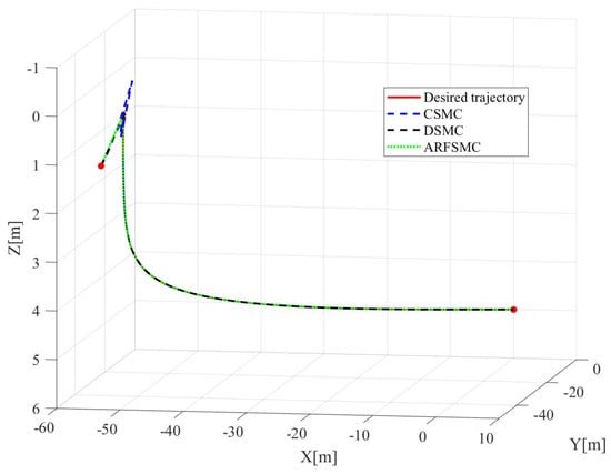
Figure 4. Three-dimensional view of the various trajectories in Simulation Case A.

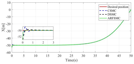
Figure 5. X-directionresulting trajectories comparison, Simulation Case A.

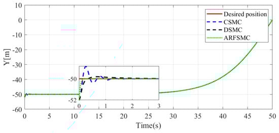
Figure 6. Y-direction resulting trajectories comparison, Simulation Case A.

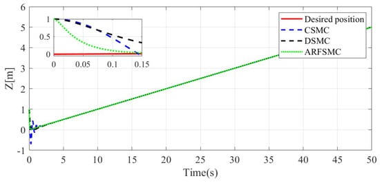
Figure 7. Z-direction resulting trajectories comparison, Simulation Case A.

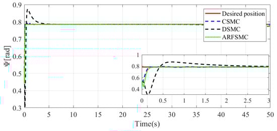
Figure 8. $\psi$-direction resulting trajectories comparison, Simulation Case A.

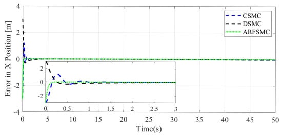
Figure 9. X-direction tracking error comparison, Simulation Case A.

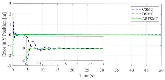
Figure 10. Y-direction tracking error comparison, Simulation Case A.

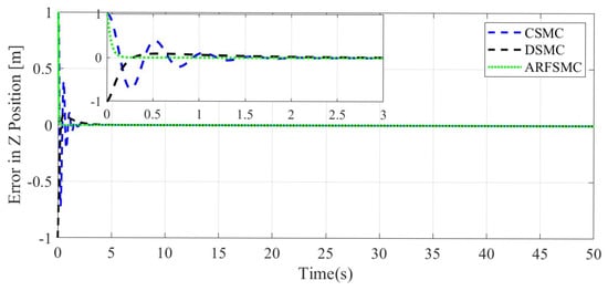
Figure 11. Z-direction tracking error comparison, Simulation Case A.

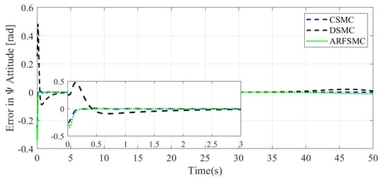
Figure 12. $\psi$-direction tracking error comparison, Simulation Case A.

Table 1. RMS tracking errors; Reduction (1/2) denotes the relative drop in tracking RMSE compared to CSMC or DSMC.

Sim. Case	Controller	Tracking RMSE, in
		$\mathit{X}$ [m]	$\mathit{Y}$ [m]	$\mathit{Z}$ [m]	$\mathit{\psi }/$[m]
A	CSMC	0.0681	0.0474	0.0248	0.0054
	DSMC	0.0654	0.0439	0.0217	0.0117
	ARFSMC	0.0571	0.0382	0.0188	0.0152
	Reduction (1/2)	16.2%/12.8%	19.4%/12.9%	24.2%/13.5%	−180.0%/−30.03%
B	CSMC	0.1006	0.0675	0.0346	0.0177
	DSMC	0.1012	0.0657	0.0335	0.0168
	ARFSMC	0.0913	0.0609	0.0303	0.0155
	Reduction (1/2)	9.2%/9.8%	9.8%/7.3%	12.4%9.5%	12.3%/7.8%
C	CSMC	0.0969	0.0648	0.0332	0.0169
	DSMC	0.0978	0.0633	0.0321	0.0159
	ARFSMC	0.0838	0.0559	0.0278	0.0139
	Reduction (1/2)	13.6%/14.3%	13.8%/11.8%	16.4%/13.5%	17.6%/12.2%

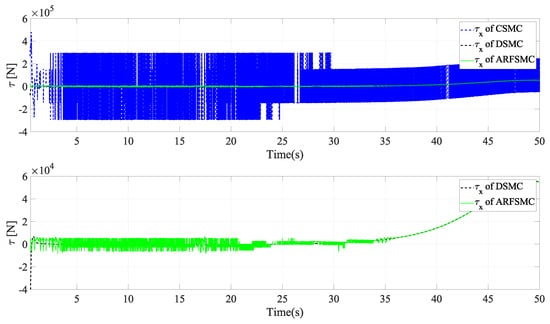
Figure 13. X-direction control signal (thruster force), Simulation Case A.

$\mathbf{TV}$ for combinations of controller type and DOF across all three simulation cases is shown in Table 2. From Table 2A, it is observed based on the TV metric that chattering in the ARFSMC control signals is 98.2%, 98.5%, 98.9%, and 98.9% lower compared to those of the CSMC in the X-, Y-, Z-, and $\psi$-direction, respectively.

Table 2. Chattering quantification metric TV evaluated for the CSMC and ARFSMC control signals; Reduction denotes relative drop in TV compared to the CSMC control signal.

Sim. Case	Controller	TV, in
		$\mathit{X}$ [N]	$\mathit{Y}$ [N]	$\mathit{Z}$ [N]	$\mathit{\psi }$ [Nm]
A	CSMC	$9.63\times {10}^9$	$9.63\times {10}^9$	$1.50\times {10}^{10}$	$9.41\times {10}^9$
	ARFSMC	$1.69\times {10}^8$	$1.40\times {10}^8$	$1.69\times {10}^8$	$1.01\times {10}^8$
	Reduction	98.2%	98.5%	98.9%	98.9%
B	CSMC	$5.65\times {10}^9$	$6.69\times {10}^9$	$8.79\times {10}^9$	$5.52\times {10}^9$
	ARFSMC	$1.92\times {10}^8$	$1.82\times {10}^8$	$2.06\times {10}^8$	$1.37\times {10}^8$
	Reduction	96.6%	97.3%	97.7%	97.5%
C	CSMC	$3.92\times {10}^9$	$3.89\times {10}^9$	$5.80\times {10}^{10}$	$3.64\times {10}^9$
	ARFSMC	$1.28\times {10}^8$	$9.93\times {10}^8$	$1.02\times {10}^8$	$7.21\times {10}^8$
	Reduction	96.7%	97.5%	98.2%	98.0%

4.2. Simulation Case B: Linear Translation with Time-Varying Mass

Once deployed to the designated mining zone, the HMV would repeatedly execute linear translations to gather mineral nodules. The HMV mass is expected to increase initially due to the intake of minerals before the transport rate catches up with the intake rate, and the HMV mass gradually decreases down to the vehicleès own mass again as the mass exchange rates reach equilibrium. In this process, the minerals onboard the HMV may cause a shift in its center of mass position, affecting the motion of the vehicle. This simulation case aims to provide a basic first-order validation of the ARFSMC under such scenarios. Thus, to simplify the analysis, the following assumptions are made:

Assumption 3.

The center of mass position of the HMV does not vary during operation.

Assumption 4.

The HMV mass is sinusoidal in time and is approximated by the function $m=m_0+150\sin \left(0.02\pi t\right)$.

The desired trajectory commanded in this simulation case is planned as Equation (39):

$$\begin{array}{c}\hfill \left\{\begin{array}{c}{x}_d\left(t\right)=0.15t\hfill \\ y_d\left(t\right)=0\hfill \\ z_d\left(t\right)=0\hfill \\ {\psi }_d\left(t\right)=0\hfill \end{array}\right.\end{array}$$

(39)

Similarly to Simulation Case A, the resulting Simulation Case B trajectories of the HMV under the three control algorithms and respective tracking errors are presented in Figure 14, Figure 15, Figure 16, Figure 17, Figure 18, Figure 19, Figure 20, Figure 21 and Figure 22. It is observed that in Simulation Case B, the tracking errors converge significantly faster with the ARFSMC than with the CSMC and DSMC. The RMS errors of the CSMC, DSMC, and ARFSMC trajectories are shown in Table 1B. Under the ARFSMC, the mean translational DOF RMS tracking error is 10.9% lower than that of the CSMC and 8.6% lower than the DSMC’s. Table 2B and Figure 23 indicates that chattering in the ARFSMC control signals is 96.6%, 97.3%, 97.7%, and 97.5% lower compared to those from the CSMC, in the X-, Y-, Z-, and $\psi$-direction, respectively. In general, the mass variation does not visibly affect the tracking results. The ARFSMC is superior compared to the CSMC and DSMC in tracking accuracy.

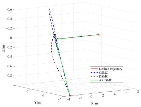
Figure 14. Three-dimensional view of the various trajectories in Simulation Case B.

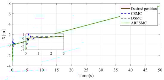
Figure 15. X-direction resulting trajectories comparison, Simulation Case B.

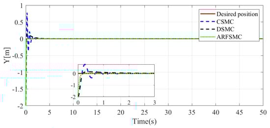
Figure 16. Y-direction resulting trajectories comparison, Simulation Case B.

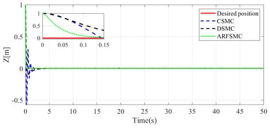
Figure 17. Z-direction resulting trajectories comparison, Simulation Case B.

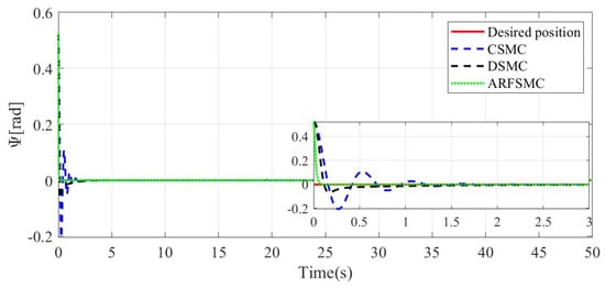
Figure 18. $\psi$-direction resulting trajectories comparison, Simulation Case B.

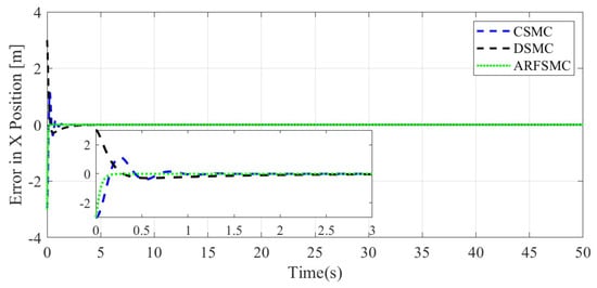
Figure 19. X-direction tracking error comparison, Simulation Case B.

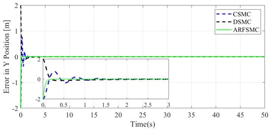
Figure 20. Y-direction tracking error comparison, Simulation Case B.

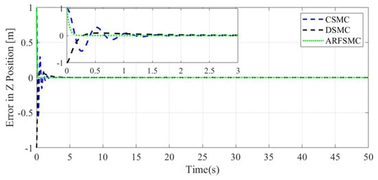
Figure 21. Z-direction tracking error comparison, Simulation Case B.

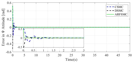
Figure 22. $\psi$-direction tracking error comparison, Simulation Case B.

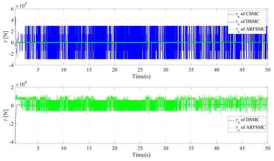
Figure 23. X-direction control signal (thruster force), Simulation Case B.

4.3. Simulation Case C: Spiral Motion

Simulation Case C concerns the maneuverability of the HMV. The mining zone seafloor terrain is likely non-planar and features protrusions; thus, it is crucial that the HMV also has a good maneuvering capability. To test this, a spiral descent trajectory is planned for the vehicle, shown in Equation (40):

$$\begin{array}{c}\hfill \left\{\begin{array}{c}{x}_d\left(t\right)=5cos(0.05\pi t-0.5\pi )\hfill \\ y_d\left(t\right)=5cos(0.05\pi t-0.5\pi )+5\hfill \\ z_d\left(t\right)=0.1t\hfill \\ {\psi }_d\left(t\right)=0.05\pi t\hfill \end{array}\right.\end{array}$$

(40)

The resulting HMV trajectories under the three control algorithms and the respective tracking errors are presented in Figure 24, Figure 25, Figure 26, Figure 27, Figure 28, Figure 29, Figure 30, Figure 31 and Figure 32. It can be observed that the convergence rates of the ARFSMC tracking errors remain high. Under the ARFSMC, the mean translational DOF RMS tracking error is 15.4% lower than that of the CSMC and 13.0% lower than the DSMC’s. Table 2C and Figure 33 indicates that chattering in the ARFSMC control signals is 96.7%, 97.5%, 98.2%, and 98.0% lower compared to the CSMC counterparts in X-, Y-, Z-, and $\psi$-direction, respectively. Overall, the ARFSMC performs satisfactorily in this simulation case.

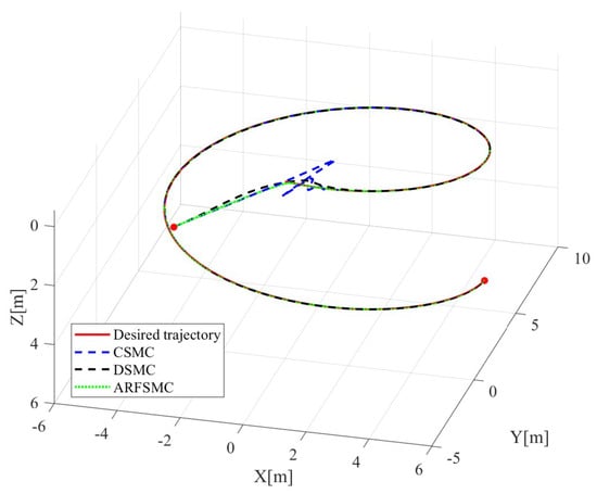
Figure 24. Three-dimensional view of the various trajectories in Simulation Case C.

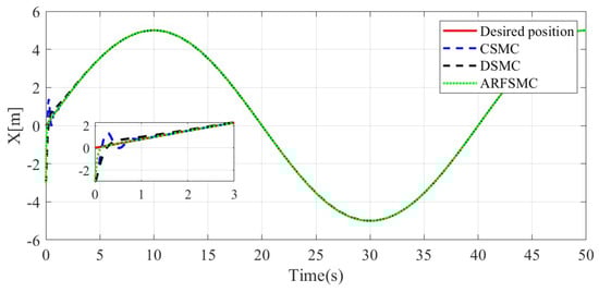
Figure 25. X-direction resulting trajectories comparison, Simulation Case C.

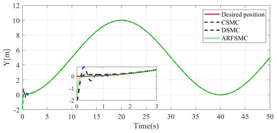
Figure 26. Y-direction resulting trajectories comparison, Simulation Case C.

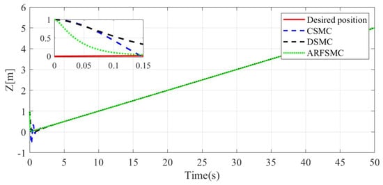
Figure 27. Z-direction resulting trajectories comparison, Simulation Case C.

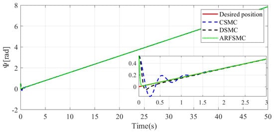
Figure 28. $\psi$-direction resulting trajectories comparison, Simulation Case C.

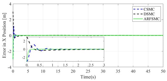
Figure 29. X-direction tracking error comparison, Simulation Case C.

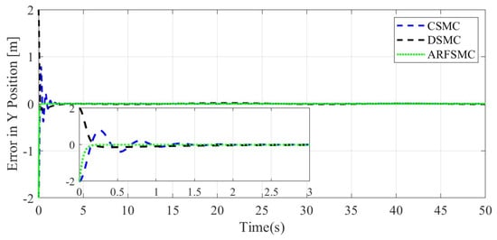
Figure 30. Y-direction tracking error comparison, Simulation Case C.

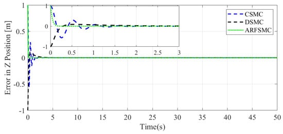
Figure 31. Z-direction tracking error comparison, Simulation Case C.

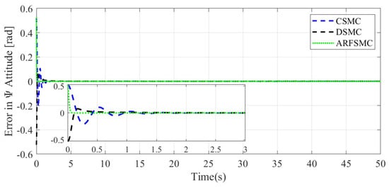
Figure 32. $\psi$-direction tracking error comparison, Simulation Case C.

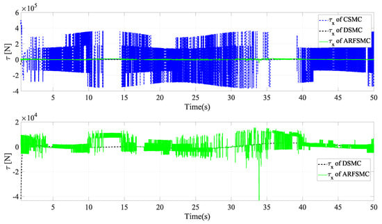
Figure 33. X-direction control signal (thruster force), Simulation Case C.

5. Conclusions

In this paper, an adaptive artificial neural network fuzzy logic sliding mode controller is developed, aimed at tracking the trajectory of a buoyancy-based deep-sea mining vehicle. The algorithm, referred to by the authors as the ARFSMC, uses an off-line trained RBFNN to generate the traditionally model-based components of the equivalent control action, and adopts an FIS switching term gain to achieve chattering alleviation. An adaptive mechanism on the RBFNN weighting matrix is included to enhance the disturbance rejection capability of the controller. To validate the effectiveness of the ARFSMC in HMV trajectory tracking, three sets of numerical simulations, based on a 4-DOF model of the vehicle and each designed to mimic a specific operation scenario, are performed, which sees the ARFSMC benchmarked against the conventional sliding mode controller (CSMC) and double-loop sliding mode controller (DSMC). Satisfactory motion control of the HMV under the ARFSMC has been observed from the simulation results, showing tracking error convergence in all degrees of freedom and smooth control signal output without high-frequency oscillations. Future directions from the current work would be to further investigate the impact of mass variation on the HMV model, as well as to introduce a disturbance observer design into the algorithm to enhance the tracking performance. A prototype vehicle will be developed based on the numerical simulations, and additional tank testing or other real-world validations will be conducted with the prototype vehicle to attain a more rigorous result of the ARFSMC tracking performance on the HMV. Furthermore, additional adaptive laws can be introduced to the RBF tunable parameters to enhance the robustness of the algorithm. It should be noted that the RBFNN used in this work has a simplified structure and lacks features like input weightings and connection thresholds found in a general RBFNN. If computational cost allows, such features afforded by the deployment of a general RBFNN model would give the ARFSMC algorithm additional flexibility.

References

- Guo, X.; Fan, N.; Liu, Y.; Liu, X.; Wang, Z.; Xie, X.; Jia, Y. Deep seabed mining: Frontiers in engineering geology and environment. Int. J. Coal Sci. Technol. 2023, 10, 23. [Google Scholar] [CrossRef]
- Kang, Y.; Liu, S. Review on the Technology and Equipment Progress and the System Scheme of Deep-Sea Mining. J. Mech. Eng. 2023, 59, 325–337. [Google Scholar]
- Levin, L.A.; Mengerink, K.; Gjerde, K.M.; Rowden, A.A.; Van Dover, C.L.; Clark, M.R.; Ramirez-Llodra, E.; Currie, B.; Smith, C.R.; Sato, K.N.; et al. Defining “serious harm” to the marine environment in the context of deep-seabed mining. Mar. Policy 2016, 74, 245–259. [Google Scholar] [CrossRef]
- Mengerink, K.J.; Van Dover, C.L.; Ardron, J.; Baker, M.; Escobar-Briones, E.; Gjerde, K.; Koslow, J.A.; Ramirez-Llodra, E.; Lara-Lopez, A.; Squires, D.; et al. A call for deep-ocean stewardship. Science 2014, 344, 696–698. [Google Scholar] [CrossRef]
- Xiao, J.; Cheng, P.; Cao, J.; Lin, R.; Luo, M.; Yu, C.; Yao, B.; Hu, Y. Dynamic analysis and simulations of a deep-sea floating mining vehicle multi-body system under real-world operating conditions. Ocean Eng. 2024, 306, 117871. [Google Scholar] [CrossRef]
- Tijjani, A.S.; Chemori, A.; Creuze, V. A survey on tracking control of unmanned underwater vehicles: Experiments-based approach. Annu. Rev. Control 2022, 54, 125–147. [Google Scholar] [CrossRef]
- Soylu, S.; Buckham, B.J.; Podhorodeski, R.P. A chattering-free sliding-mode controller for underwater vehicles with fault-tolerant infinity-norm thrust allocation. Ocean Eng. 2008, 35, 1647–1659. [Google Scholar] [CrossRef]
- Slotine, J.J.E. Sliding controller design for non-linear systems. Int. J. Control 1984, 40, 421–434. [Google Scholar] [CrossRef]
- Bessa, W.M.; Dutra, M.S.; Kreuzer, E. An adaptive fuzzy sliding mode controller for remotely operated underwater vehicles. Robot. Auton. Syst. 2010, 58, 16–26. [Google Scholar] [CrossRef]
- Eun, Y.; Kim, J.H.; Kim, K.; Cho, D.I. Discrete-time variable structure controller with a decoupled disturbance compensator and its application to a CNC servomechanism. IEEE Trans. Control Syst. Technol. 1999, 7, 414–423. [Google Scholar]
- Slotine, J.J.; Sastry, S.S. Tracking control of non-linear systems using sliding surfaces, with application to robot manipulators. Int. J. Control 1983, 38, 465–492. [Google Scholar] [CrossRef]
- Chung, S.C.Y.; Lin, C.L. A transformed Lure problem for sliding mode control and chattering reduction. IEEE Trans. Autom. Control 1999, 44, 563–568. [Google Scholar] [CrossRef]
- Wang, Y.; Zhang, M.; Wilson, P.A.; Liu, X. Adaptive neural network-based backstepping fault tolerant control for underwater vehicles with thruster fault. Ocean Eng. 2015, 110, 15–24. [Google Scholar] [CrossRef]
- Qiao, L.; Zhang, W. Double-loop integral terminal sliding mode tracking control for UUVs with adaptive dynamic compensation of uncertainties and disturbances. IEEE J. Ocean. Eng. 2018, 44, 29–53. [Google Scholar] [CrossRef]
- Li, J.; Guo, H.; Zhang, H.; Yan, Z. Double-loop structure integral sliding mode control for UUV trajectory tracking. IEEE Access 2019, 7, 101620–101632. [Google Scholar] [CrossRef]
- Huang, B.; Yang, Q. Double-loop sliding mode controller with a novel switching term for the trajectory tracking of work-class ROVs. Ocean Eng. 2019, 178, 80–94. [Google Scholar] [CrossRef]
- Xia, Y.; Xu, K.; Li, Y.; Xu, G.; Xiang, X. Adaptive trajectory tracking control of a cable-driven underwater vehicle on a tension leg platform. IEEE Access 2019, 7, 35512–35531. [Google Scholar] [CrossRef]
- Yang, M.; Sheng, Z.; Yin, G.; Wang, H. A recurrent neural network based fuzzy sliding mode control for 4-DOF ROV movements. Ocean Eng. 2022, 256, 111509. [Google Scholar] [CrossRef]
- Wang, Z.; Liu, Y.; Guan, Z.; Zhang, Y. An adaptive sliding mode motion control method of remote operated vehicle. IEEE Access 2021, 9, 22447–22454. [Google Scholar] [CrossRef]
- Fossen, T.I. Guidance and Control of Ocean Vehicles; Wiley: Chichester, UK, 1999. [Google Scholar]
- Zhang, M.J.; Chu, Z.Z. Adaptive sliding mode control based on local recurrent neural networks for underwater robot. Ocean Eng. 2012, 45, 56–62. [Google Scholar] [CrossRef]
- Chu, Z.; Chen, Y.; Zhu, D.; Zhang, M. Observer-based adaptive neural sliding mode trajectory tracking control for remotely operated vehicles with thruster constraints. Trans. Inst. Meas. Control 2021, 43, 2960–2971. [Google Scholar] [CrossRef]
- Peng, Z.; Wang, J. Output-feedback path-following control of autonomous underwater vehicles based on an extended state observer and projection neural networks. IEEE Trans. Syst. Man Cybern. Syst. 2017, 48, 535–544. [Google Scholar] [CrossRef]
- Li, J.; Du, J.; Chen, C.P. Command-filtered robust adaptive NN control with the prescribed performance for the 3-D trajectory tracking of underactuated AUVs. IEEE Trans. Neural Netw. Learn. Syst. 2021, 33, 6545–6557. [Google Scholar] [CrossRef] [PubMed]
- Xiang, X.; Yu, C.; Lapierre, L.; Zhang, J.; Zhang, Q. Survey on fuzzy-logic-based guidance and control of marine surface vehicles and underwater vehicles. Int. J. Fuzzy Syst. 2018, 20, 572–586. [Google Scholar] [CrossRef]
Disclaimer/Publisher’s Note: The statements, opinions and data contained in all publications are solely those of the individual author(s) and contributor(s) and not of MDPI and/or the editor(s). MDPI and/or the editor(s) disclaim responsibility for any injury to people or property resulting from any ideas, methods, instructions or products referred to in the content. |
© 2025 by the authors. Licensee MDPI, Basel, Switzerland. This article is an open access article distributed under the terms and conditions of the Creative Commons Attribution (CC BY) license (https://creativecommons.org/licenses/by/4.0/).