Abstract
Marine ship-radiated noise and multipath Doppler effect reduce the positioning accuracy of linear frequency modulation (LFM) signals in ocean waveguide environments. However, the assumption of Gaussian noise underlying most time–frequency domain algorithms limits their effectiveness in mitigating non-Gaussian interference. To address this issue, we propose a Deep-separable Conformer Wave-Unet (DC-WUnet)-based underwater acoustic signal enhancement network designed to reconstruct signals from interference and noise. The encoder incorporates the Conformer module and skip connections to enhance the network’s multiscale feature extraction capability. Meanwhile, the network introduces depthwise separable convolution to reduce the number of parameters and improve computational efficiency. The decoder applies a slope-based linear interpolation method for upsampling to avoid introducing high-frequency noise during decoding. Additionally, the loss function employs joint time–frequency domain constraints to prevent signal loss and compression, particularly under low Signal-to-Noise Ratio (SNR) conditions. Experimental evaluations under an SNR of −10 dB indicate that the proposed method achieves at least a 32% improvement in delay estimation accuracy and a 2.3 dB enhancement in output SNR relative to state-of-the-art baseline algorithms. Consistent performance advantages are also observed under varying SNR conditions, thereby validating the effectiveness of the proposed approach in shipborne noisy environments.
1. Introduction
In marine hydroacoustic positioning systems [1], the distance and position of a target are determined by the time delay in signal propagation [2]. With the growing number of vessels and the increased deployment of detection equipment on ships, radiated ship noise has emerged as a major source of interference [3]. In particular, high-noise environments dominated by propeller and mechanical noise can severely degrade signal quality and compromise positioning accuracy [4]. Furthermore, multipath Doppler interference distorts both the time-domain waveform and frequency-domain characteristics of received signals, resulting in significant localization errors. Therefore, enhancing hydroacoustic signals and suppressing radiated noise are key to improving the performance of hydroacoustic positioning systems [5].
To address the aforementioned challenges, various signal enhancement techniques have been proposed, which can be broadly classified into frequency-domain and time-domain approaches. Frequency-domain methods—such as Continuous Wavelet Transform (CWT) [6], spectral subtraction [7], and adaptive filtering [8]—aim to suppress noise by analyzing spectral characteristics and removing noise components. However, these techniques often perform poorly in complex or unknown noise environments and may introduce phase distortions that compromise signal integrity [9]. Time-domain methods, by contrast, operate directly on raw signal sequences and thus avoid the structural distortion inherent in frequency-domain transformations. Typical examples include Variational Mode Decomposition (VMD) [10] and K-Singular Value Decomposition (K-SVD) [11], which are effective in extracting structural features and reconstructing clean signals. Nonetheless, their performance remains limited under non-stationary noise and multipath Doppler interference in underwater environments [12].
Deep learning methods have demonstrated significant advantages in time-domain signal processing by extracting multi-dimensional features from raw signals through convolutional kernels [13]. However, most existing deep learning models for signal enhancement rely on stacked multi-layer convolutional architectures, which often struggle to effectively preserve and transmit multiscale and global information across layers. This limitation hampers the network’s ability to simultaneously capture global context and fine-grained local details, potentially resulting in signal distortion and the loss of high-frequency components [14,15]. Moreover, some models suffer from high parameter complexity and slow inference speeds, making them unsuitable for real-time sonar applications. To improve robustness under diverse signal and noise conditions, it is also essential to integrate both time- and frequency-domain information.
To address these challenges, we present a lightweight hydroacoustic signal enhancement network that integrates time–frequency domain features while maintaining strong representational capacity and computational efficiency. The proposed method is tailored to mitigate shipborne radiated noise and multipath Doppler interference, thereby improving the accuracy of underwater range measurements. The main contributions of this work are as follows:
- (1)
- A DC-WUnet network model is proposed, which employs an encoder-decoder structure to separate clean signals from ship noise and multipath Doppler effect interference, thereby enhancing the target signal.
- (2)
- In the encoder, the Conformer module and skip connections enhance the network’s ability to capture signal features. Multi-scale features are extracted through feature transfer facilitated by skip connections and convolutional kernels of varying sizes in each encoding layer. Additionally, depthwise separable convolutions are introduced to address the feature loss associated with traditional downsampling methods while reducing network parameters and improving computational efficiency. In the decoder, a slope-based linear upsampling method delivers superior reconstruction performance, particularly in regions of the signal with rapid variations.
- (3)
- In the network loss function, frequency-domain processing is introduced, and by performing joint computation in the time–frequency domain, the problem of information compression and loss caused by the inability to extract clean signals in the time domain is addressed.
2. Related Work
In recent years, time-domain and frequency-domain methods have been extensively applied and researched for noise suppression and signal quality enhancement in hydroacoustic signals. Kumar et al. [16] proposed a denoising algorithm for non-Gaussian non-smooth signals that employs a Continuous Wavelet Transform with Linear Frequency Modulation (LFM) [17]. However, the denoising performance depends on the time-frequency parameters, which must be tuned manually [18], and the robustness is poor. Li et al. [19] proposed a method that integrates a priori Sub-Bottom Profiler (SBP) information with a Variational Mode Decomposition (VMD) framework. This solves the problem of manual parameter tuning and provides good robustness, but it faces difficulties in obtaining a priori information for complex marine environments. Xiao et al. [20] proposed a signal denoising method that employs VMD with a CWT. VMD is used to decompose the signal using Variational Mode Functions (VMFs), and then the denoising of each VMF is achieved using wavelet soft-thresholding [21]. While the algorithm demonstrates strong generalization capability, its use of wavelet soft-thresholding may lead to the unintended removal of useful signal components along with noise, which can result in distortion during signal reconstruction. Additionally, the VMD decomposition involves complex computations and lengthy processing times, making it less suitable for real-time applications, such as underwater acoustic positioning systems. Yang et al. [22] proposed a denoising algorithm integrating variational mode decomposition, multiscale entropy, wavelet thresholding, and Savitzky–Golay filtering, which enhances the suppression of interference signals. However, it remains limited in handling channel interferences such as multipath Doppler effects in marine environments, and suffers from high computational complexity and low efficiency. Wu et al. [23] proposed a low-frequency underwater acoustic signal denoising method based on sparse decomposition and learning via a Discrete Cosine Transform (DCT) [24]. It employs Orthogonal Matching Pursuit (OMP) and K-Singular Value Decomposition to sparsely represent the signal, update the dictionary, and then reconstruct the signal. Nonetheless, the algorithm’s performance heavily relies on the quality of the initial dictionary, and an inappropriate choice can easily cause convergence to a local optimum [25]. Furthermore, the algorithm has relatively high computational complexity, which makes it difficult to apply in real-time localization systems.
Deep learning has recently been proposed for signal denoising. It uses a large amount of noisy data to extract features and model complex structures for signal identification and reconstruction. Gogna et al. [26] proposed a method for signal reconstruction, in which a Stacked Auto Encoder (SAE) [27] was employed. Despite its strengths, a key limitation of this architecture is that the features extracted by each encoding layer are not directly available to the corresponding decoding layers. This lack of inter-layer communication hinders the decoder’s ability to incorporate additional feature constraints during reconstruction, which may lead to signal distortion. Russo et al. [28] proposed an improved denoising autoencoder capable of recovering signal waveforms under various noise conditions, though its feature extraction remains limited in complex marine environments. Guimarães et al. [29] employed a Wave-Unet network [30] for feature extraction and signal enhancement. One limitation of the model arises from the encoder’s use of fixed-size convolutional kernels, which restricts its ability to capture features at varying spatial scales and adversely affects multiscale feature representation. Under complex ocean conditions with low signal-to-noise ratios, the algorithm struggles to effectively capture useful components of the signal, which leads to signal distortion during reconstruction in the decoder. Further, some signal features are discarded during downsampling, which introduces high-frequency artifacts in the reconstructed signal. Chu et al. [31] proposed a deep learning-based high-gain method for underwater acoustic signal detection in environments with intensity fluctuations, in which the Conv-Tasnet framework [32] was employed to extract, separate, and reconstruct signals through its encoder, separator, and decoder modules, respectively. A limitation of this model is that the separation layer employs a stacked convolutional structure, resulting in a substantial increase in the number of parameters and reduced computational efficiency. Additionally, there is no information sharing between the encoder and decoder within the same layer. This structure fails to effectively facilitate information transfer, leading to distortion during signal reconstruction by the decoder.
3. Ranging Signal Simulation Model
3.1. Ship-Radiated Noise Modeling
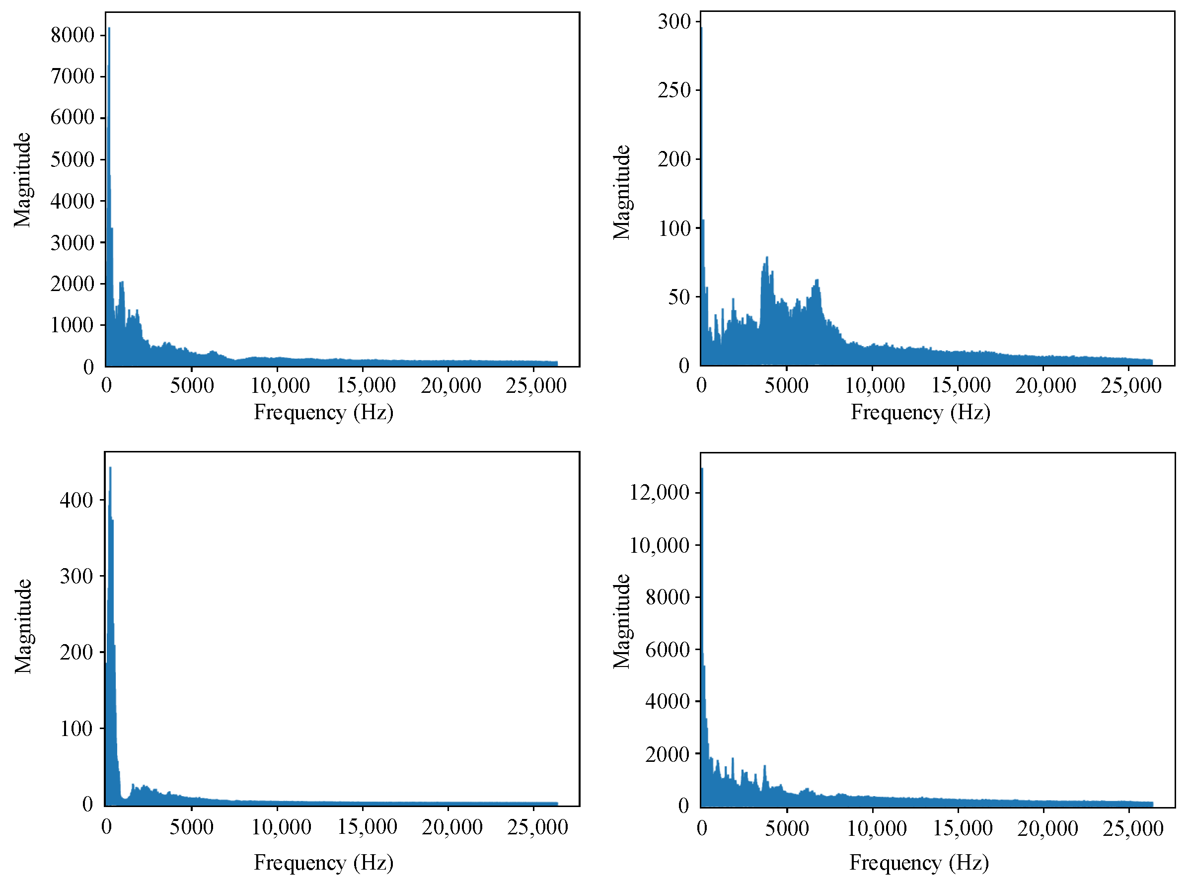
Ship-radiated noise primarily results from the superposition of continuous and line spectra, with mechanical and propeller noise being its main sources. This study uses the Deepship [33] dataset to ensure the reliability of the research findings. The dataset, which contains real ship noise data, is also used to verify the practicality and robustness of the network. The dataset contains 47 h and 4 min of actual underwater recordings, with data collected over nearly 29 months at measurement sites throughout the year. Figure 1 presents the spectral analysis results obtained from random sampling of the Deepship dataset in the frequency domain. The analysis clearly shows that the noise spectrum within the Deepship dataset exhibits typical characteristics of marine environmental noise, encompassing frequency components originating from diverse noise sources.
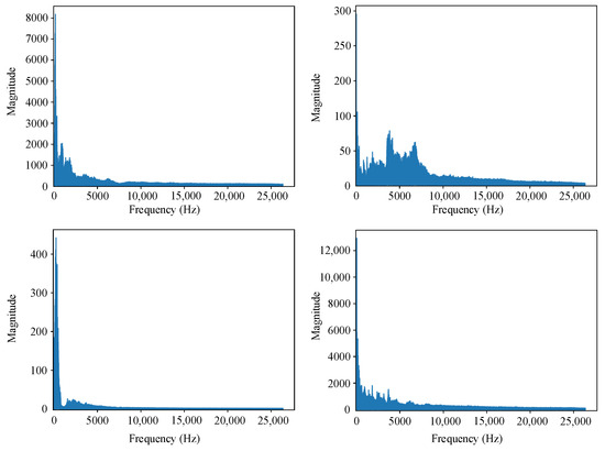
Figure 1.
Frequency domain spectrum of the deepship noise dataset.
3.2. Interference Signal Model
The BELLHOP ray acoustic model is used to simulate the Underwater Acoustic (UWA) channel environment [34]. In this study, we apply the BELLHOP model in combination with the measured marine environmental dataset SWellEx-96 to emulate the underwater acoustic channel more realistically. This approach enables the simulation of ocean noise and channel interference under real-world conditions. A schematic illustration of the BELLHOP model appears in Figure 2.
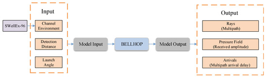
Figure 2.
Schematic of the BELLHOP model.
In marine environments, LFM signals exhibit the advantages of slow signal attenuation and strong penetration, making them widely applicable in underwater acoustic positioning and signal synchronization. To better reflect real-world conditions, this study selects the LFM signal as the target signal. The LFM signal used in this work is defined as follows:
where A is the amplitude, is the starting frequency, is the FM slope, is the initial phase, n is the index of the discrete signal, N is the total number of sampling points, is the sampling rate, and is the discrete time points.
The underwater acoustic channel model simulated by the BELLHOP model is used to simulate the received signal of the LFM signal propagating in the real underwater acoustic channel, taking into account ray attenuation, the multipath effect [35], and the Doppler effect [36]. The received signal is given by
where and are the direct path amplitude and delay for the BELLHOP model, and is the Doppler shift of the direct path. The multipath interference is
where N is the number of multipath signals, and are the amplitude and delay of the ith path, respectively, which are obtained through BELLHOP. is the Doppler shift [37] for the i-th path that causes a modulation of the signal [38], represented by the term
where is the Doppler shift for the i-th path, which can be calculated based on the relative velocity between the transmitter, receiver, and the propagation medium, in conjunction with the Doppler formula [39]
where represents the sound speed in water, is the receiver’s velocity, and is the transmitter’s velocity. When the target’s velocity relative to the receiver is much smaller than , a first-order approximation can be used
where v is the relative velocity along the wave propagation direction. The relative velocity can be expressed as the sum of the ship’s speed and the flow speed, multiplied by the relative angle. Since the arrival angle of the signal differs for each path, the arrival angle for each propagation path is approximated using BELLHOP, which replaces the relative angle, thereby allowing the calculation of the Doppler frequency shift for the signal on each path [40]
where is the relative vessel speed between the ship and the receiver, and is the relative ocean current speed between the ship and the receiver. The combination of vessel speed and ocean current speed is necessary because when they move in the same direction, the vessel’s speed increases, resulting in a higher relative sound speed in water. Conversely, if they are in opposite directions, the current partially cancels out the effect of the vessel’s speed. is the speed of sound in water, and it serves as a conversion factor to align the motion velocities with the actual propagation speed of sound. For simplicity, the sound speed is set to 1500 m/s in this paper. is the arrival angle of the sound wave when it reaches the receiver, which is obtained through BELLHOP [41] by considering the Channel Environment (), Detection Distance (), and Launch Angle (). The includes the water’s temperature, salinity, depth, and other factors that influence sound propagation in the medium, affecting the wave’s path and refraction. refers to the distance between the sound source and the receiver. is the angle at which the sound wave is emitted relative to a reference plane.
To simulate its effect on the received acoustic signal, ship-radiated noise was introduced into the model. The interfering signal after noise addition is given by
where is radiated noise from ships, obtained from the deepship dataset, and is the simulated interference signal.
4. DC-WUnet Network
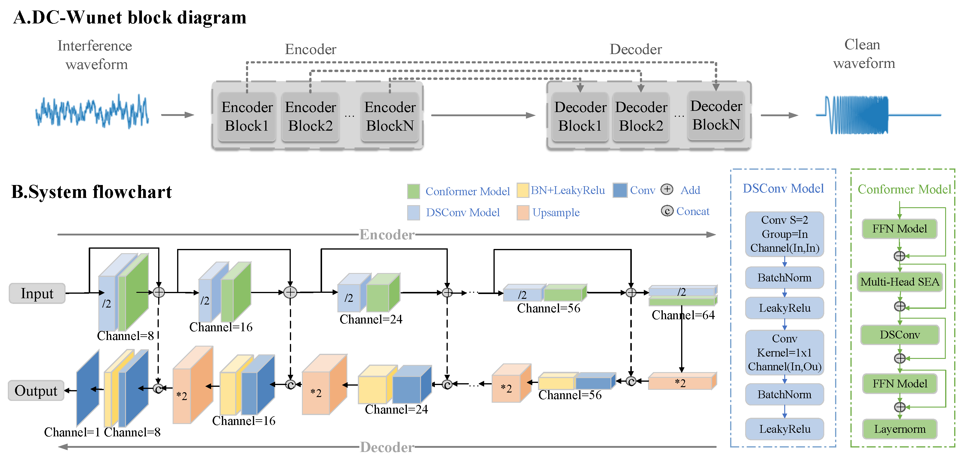
Figure 3A indicates that the DC-WUnet network takes the time-domain waveform of the interfering noise signal as input and outputs the filtered noise target signal after going through the coding and decoding layers. Figure 3B presents the DC-WUnet structure. In the encoder, multiple encoding blocks are used, each consisting of a Depthwise Separable Convolution (DSConv) and a Conformer module. Skip connections transmit features from one encoding block to the next, enhancing feature propagation and mitigating information loss. In the decoder, each decoding block corresponds one-to-one with an encoding block and comprises an upsampling module followed by a convolutional module. These modules integrate the features transmitted from the encoder to reconstruct the target signal. The encoder module has L layers, with each layer halving the temporal resolution and doubling the feature resolution, while the decoder does the opposite.
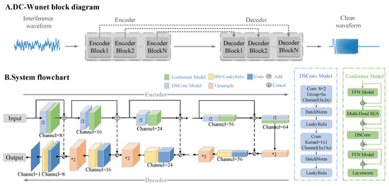
Figure 3.
(A) A block diagram of the DC-WUnet system. The encoder is used to recognize the target signal in the noise signal and extract its feature information, and the decoder reconstructs the target signal based on the extracted signal features. (B) A flowchart of the proposed system. Each encoding block consists of a Conformer module and a depth-separable convolution, and the decoding block consists of a down-adoption module and a convolution module.
DSConv consists of a depth convolution and a point convolution. The number of depth convolution groups is equal to the number of channels, the step size is 2, and the point convolution has a kernel size of 1. The Conformer uses a feedforward module, a multi-attention module, a convolution module, and normalization. UpSample uses slope-based interpolation with doubled temporal resolution. Concat links the currently extracted features with local features, and Add combines these features.
The proposed network parameters are given in Table 1, where e and d represent the coding and decoding layers, respectively, and are the input and output dimensions of the corresponding coding and decoding layers, is the time-domain signal length, is the number of coding and decoding layers, and is the initial number of input passes.

Table 1.
The block diagram of the DC-WUnet architecture illustrates the module composition, arrangement, connection patterns, and key parameters of the encoder and decoder layers while also depicting the data flow and the changes in feature map dimensions throughout the model.
4.1. Loss Function
Most deep learning-based signal enhancement algorithms rely solely on time-domain loss functions during training, which introduces certain limitations. Under high signal-to-noise ratio (SNR) conditions, when the network fails to effectively extract target signal features from interference, it tends to minimize the loss by decreasing the amplitude of the generated signal. This often results in signal distortion or even the omission of important signal components. To address this issue, this paper proposes a joint loss constraint strategy that incorporates both time-domain and frequency-domain losses, thereby guiding the network to preserve signal integrity and mitigating the distortion caused by reliance on time-domain loss alone. The time–frequency domain joint loss function is defined as
where is the time-domain loss Mean Square Error (MSE), is the frequency-domain loss MSE, and and are the time-domain and frequency-domain loss weights with
where is the number of time-domain samples, denotes the Fourier Transform (FT), is the clean hydroacoustic signal without noise and interference, and is the received hydroacoustic signal after network processing.
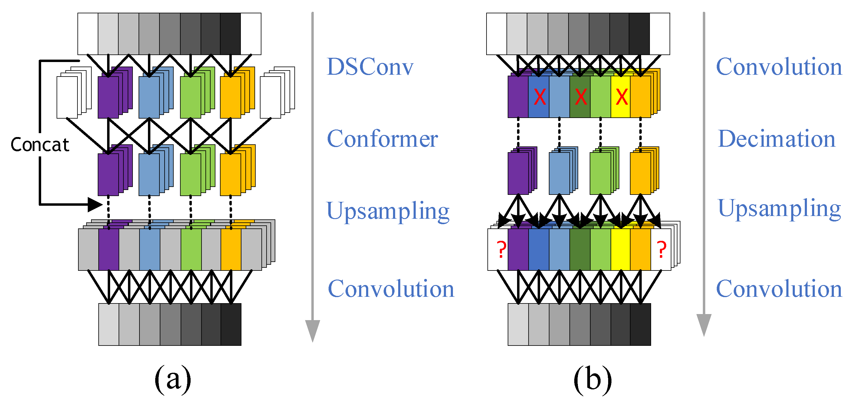
4.2. Upsampling and Downsampling
Convolution and discard operations are typically used for upsampling and downsampling along the time dimension, as shown in Figure 4b. During upsampling, convolution with zero padding extends the time dimension but also introduces high-frequency noise. From the frequency domain perspective, the multipath and Doppler effects cause distortion of the signal’s frequency components. The use of zero padding further inserts artificial zero values into these distorted frequency components, resulting in spectral discontinuities. These discontinuities produce spurious frequency components, which hinder the network’s ability to accurately reconstruct the signal’s frequency information.
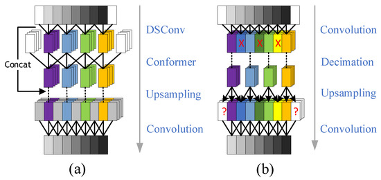
Figure 4.
Optimization diagram for upsampling and downsampling modules. (a) Shows the optimized module diagram; (b) shows the pre-optimized module diagram.
During downsampling, directly discarding data leads to the loss of critical signal features and causes distortion in the reconstructed waveform. To address this, depthwise separable convolutions are employed for downsampling in the time domain to preserve signal integrity while reducing computational complexity. This addresses the high-frequency distortion caused by feature loss, where the depthwise convolution, by performing independent convolutions on each signal component, better preserves its unique time-domain features and prevents feature loss due to signal overlap or interference.
Additionally, pointwise convolutions capture the correlation between the time and feature dimensions more effectively, providing richer and more discriminative features. This property is particularly critical in frequency domain recovery, as there are complex dependencies between frequency components. Pointwise convolutions can uncover the relationships between different frequency components, thereby better restoring the signal’s frequency characteristics.
Furthermore, using interpolation instead of convolution for upsampling ensures temporal continuity after interpolation. This addresses the aliasing problem caused by convolutional padding, which can lead to distortion or loss of certain frequency components in the signal. It also mitigates the introduction of discontinuous frequency components in the frequency domain due to padding, thereby preserving spectral continuity. Traditional linear interpolation computes the average of two adjacent points; however, abrupt amplitude changes when the target signal arrives or departs often introduce high-frequency noise during the interpolation process. To address this issue, this paper proposes a novel interpolation method that incorporates slope information to adjust interpolation parameters, thereby providing a more accurate fit to signal variations. The interpolation function is given by
where is the interpolated feature, and are the local features, M is the local range which is used to determine the slopes for the features of the subsequent M samples, and is the sigmoid function which constrains to the interval [0, 1]. This interpolation is close to when the slope is large and to when it is small; thus, it mitigates the high-frequency noise introduced before and after the signal. The proposed structure is shown in Figure 4a.
4.3. Skip Connections and Conformer Model
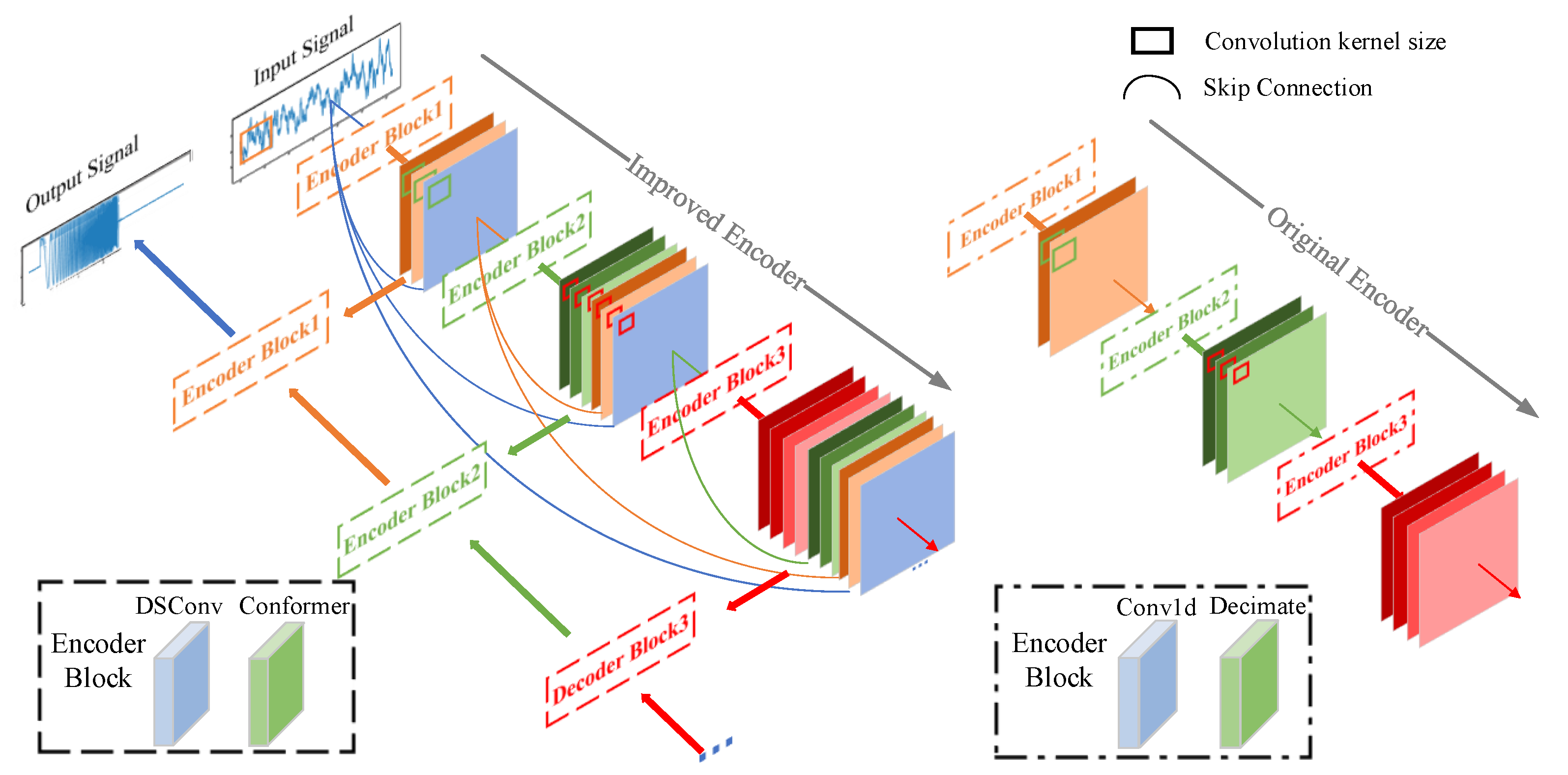
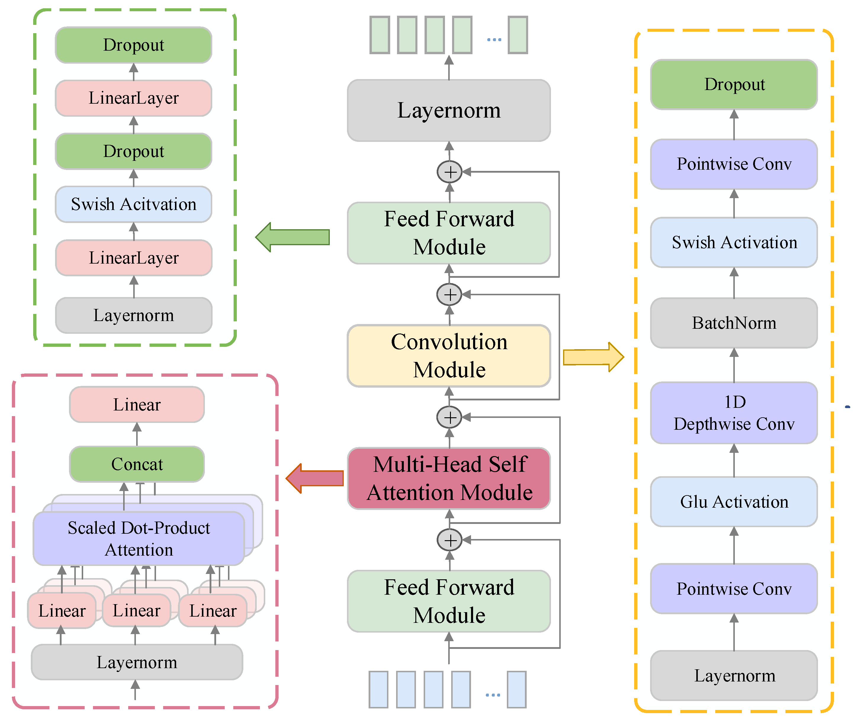
In Figure 5, the improved encoding layer introduces skip connections to pass signal features extracted at each layer to the subsequent encoding layer. Due to varying convolution kernel sizes and feature extraction scales across layers, this design enables multiscale feature extraction and improves the representation of the transmitted features. This not only provides the network with multiscale feature information—facilitating the identification of ship noise components and target signals—but also supplies more detailed features during decoding and reconstruction, enabling the recovery of cleaner signals. The Conformer module [42] shown in Figure 6 is composed of Feed Forward (FF) modules, a multi-head self-attention module, and a convolution module.
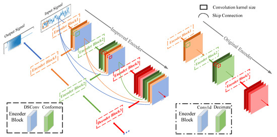
Figure 5.
Comparison of coding layers before and after improvement.
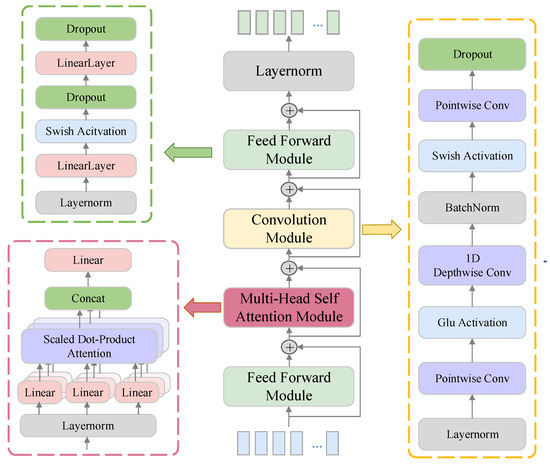
Figure 6.
Structure of the Conformer Module.
4.3.1. Feed Forward Module
The FF module captures the local features of the signal through a nonlinear transformation while modeling the continuous spectrum noise in the ship noise, thereby effectively distinguishing between noise features and signal features. Simultaneously, its capacity for high-dimensional projection and channel expansion enables the compensation for missing or attenuated frequency components in the spectrum, thereby improving the completeness and accuracy of the signal’s frequency domain representation. The FF module consists of two linear transformation layers and a Swish activation function [43]
where x is the input, and are the weights, and and are the biases obtained during training.
4.3.2. Multi-Head Self-Attention Module
In contrast to the FF module, which captures local features and noise modeling, the multi-head self-attention module is able to capture global feature relationships in the signal. Noise features of specific frequencies in line spectral noise are recognized in its multi-head structure through the attention mechanism. By combining the local features extracted in the FF module, higher weights are given to the global and local features of hydroacoustic signals, whereas lower weights are given to the local and global features of ship noise.
Meanwhile, the multi-head self-attention mechanism computes attention weights between different feature channels and time steps. This enables the extraction of global frequency patterns from the temporal characteristics of the input signal. It then decomposes these patterns into multiple frequency domain components, with multiple attention heads learning different frequency dependencies to capture and restore the target frequency components. Finally, the useful frequency components are weighted and combined to recover the original signal frequency. The module consists of a self-attention mechanism and a multi-head mechanism. The input sequence x undergoes three linear transformations to obtain the representations
where are the weight matrices. Then, the result for attention head i is obtained using the Softmax activation function [44]
where denotes the dimensional scaling factor used to stabilize the dot-product attention. In this work, a three-head, self-attention module is employed with scaling factors 2, 2, and 4, respectively. The superscript T denotes transpose.
4.3.3. Convolution Module
The global and local features of the target signals obtained by the FF module and the multi-attention self-attention module are combined with the weight information to reconstruct the clean signals and remove the radiated noise from the ship. It employs two point-by-point convolutions and one deep convolution. The activation functions used are Glu [45] and Swish, and then Batch normalization [46] is performed. The point-by-point convolution kernel is 1×1 with a step size of 1, and the deep convolution kernel is 3 × 3 with a step size of 1.
5. Experiment Setup
5.1. Dataset
To evaluate the performance of the constructed model, 15,000 hydroacoustic signals with measured ship-radiated noise (as described above) and channel interference were simulated under different SNR environments using the signal model described in Section 3.2. From these signals, 13,000 were randomly selected for training, 1000 for validation, and the remaining 1000 for testing. Each signal was sampled at 48 kHz. The simulation parameters are provided in Table 2. Additionally, the direct path delay values were obtained using BELLHOP, which served as the ground truth for delay estimation accuracy in the subsequent network enhancement evaluation.
Table 2.
Simulation parameters required for generating interference signals in a complex marine environment (Section 3.2), including LFM signal simulation parameters and multipath Doppler effect simulation settings.
5.2. Experimental Configuration and Training Goal
For training, the samples were truncated to a length of L = 1500. The loss parameters are and . The Adam optimizer [47] was used with a learning rate of , decay rates of and , a Batchsize of , and 100 epochs. The training algorithm is given in Algorithm 1.
| Algorithm 1: Network Training Algorithm |
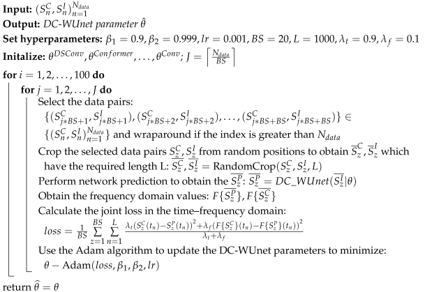 |
5.3. Evaluation Metrics
Two metrics were used for performance evaluation. The Time of Arrival (TOA) error is given by
where is the direct path delay of the clean signal, and is the corresponding delay of the received signal after network processing:
where is the signal correlation at time t, is the clean hydroacoustic signal, is the received signal after network processing, and is the length of the signal. The average TOA error is then
where is the number of test samples.
The specific flowchart for calculating TOA accuracy and error distribution is shown in Figure 7. The SNR is given by
where is the clean signal power, and is the received signal power before and after network processing:
where j = I or P; that is, represents the SNR of the signal after algorithmic enhancement, and represents the SNR of the interference signal.
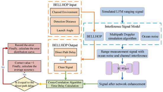
Figure 7.
The flowchart for calculating TOA accuracy and error distribution.
5.4. Comparison Algorithms
In our experiments, we compare the proposed method with five existing approaches introduced in Section 2, including the VMD-CWT method proposed by Xiao, the K-SVD method by Wu, the SAE method by Gogna, the Wave-Unet method by Guimarães, and the Conv-Tasnet method by Chu. These methods were selected due to their widespread use and strong performance in the recent signal enhancement literature. To ensure a fair comparison, all methods are evaluated under the same conditions, including the dataset and evaluation metrics.
6. Experiments and Results
6.1. Training Results
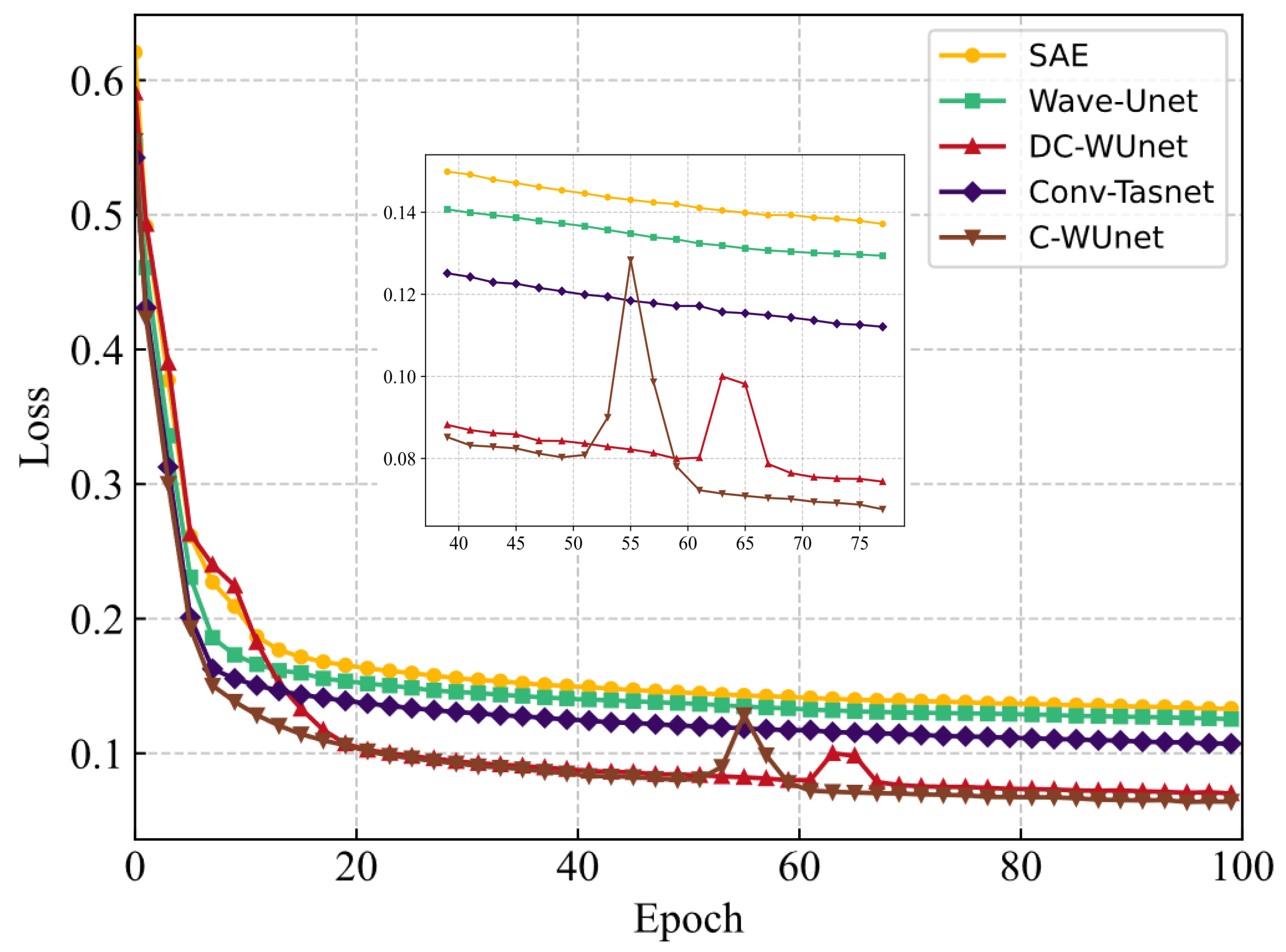
Figure 8 presents the network training loss for five methods with ship-radiated noise, multipath, and Doppler interference at SNR = −10 dB. The results show that the loss increases slightly after 50 epochs due to the introduction of frequency domain loss, which suppresses the amplitude of the compressed signal in the time domain. In the early stages of training, time-domain loss dominates, while in the later stages, frequency-domain loss becomes dominant.
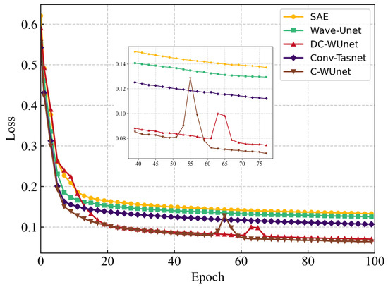
Figure 8.
Training loss for five networks at SNR = −10 dB.
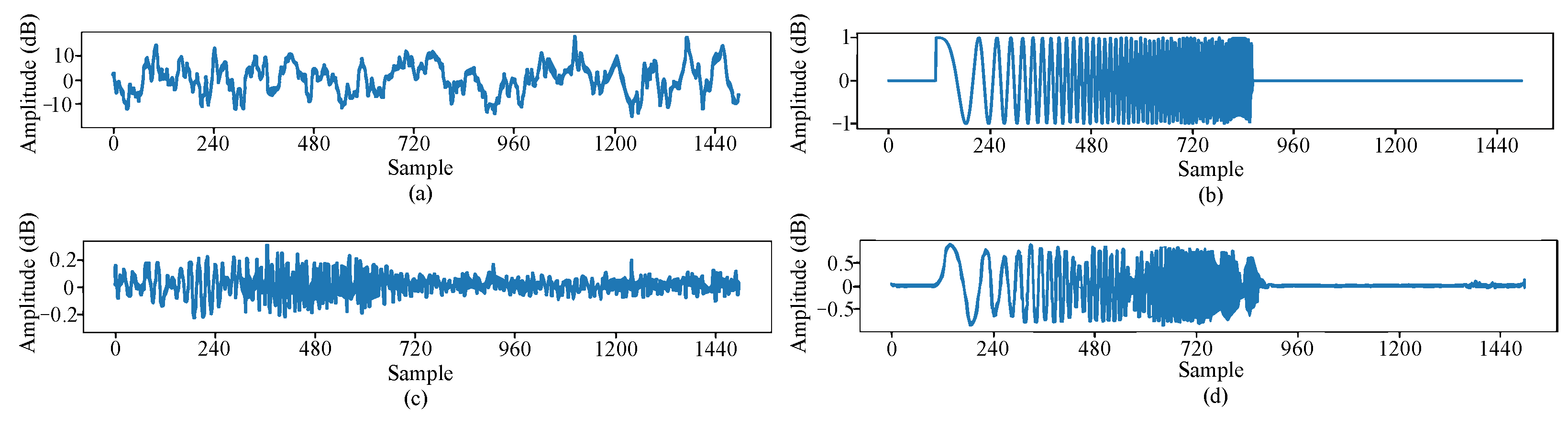
By applying network models trained separately in the time domain and the time–frequency domain to the same data within a common test set, the effectiveness of incorporating frequency-domain loss is evaluated. The results are shown in Figure 9. Figure 9a shows the received hydroacoustic signal with ship-radiated noise, multipath, and Doppler interference at SNR = −10 dB. The corresponding clean signal is given in Figure 9b. The network output after time-domain training is shown in Figure 9c, where the amplitude of the reconstructed signal is only 0.25 dB. This occurs because when the network fails to extract the target signal features, it compresses the signal’s time-domain amplitude to reduce the loss, resulting in signal distortion. After joint time–frequency domain training, the enhanced network performance is depicted in Figure 9d. A comparison with enhancement solely through time-domain training shows significant improvements in the signal waveform, approaching the clean signal. Regarding signal amplitude, the network enhanced with joint frequency-domain training achieves amplitudes ranging approximately from —0.5 to 0.5 dB. In contrast, the amplitude of the signal enhanced with time-domain training only reaches around —0.2 to 0.2 dB. This improvement indicates alleviation of amplitude compression issues.
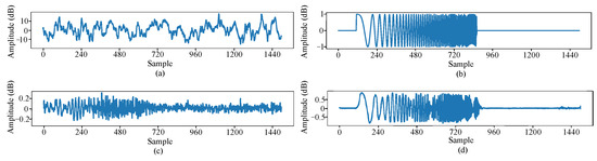
Figure 9.
Signals before and after joint time–frequency domain training using DC-WUnet. (a) is a clean signal, (b) is an interference signal, (c) is the enhancement effect of the network trained in the time domain, and (d) is the enhancement effect of the network trained jointly in the time-frequency domain.
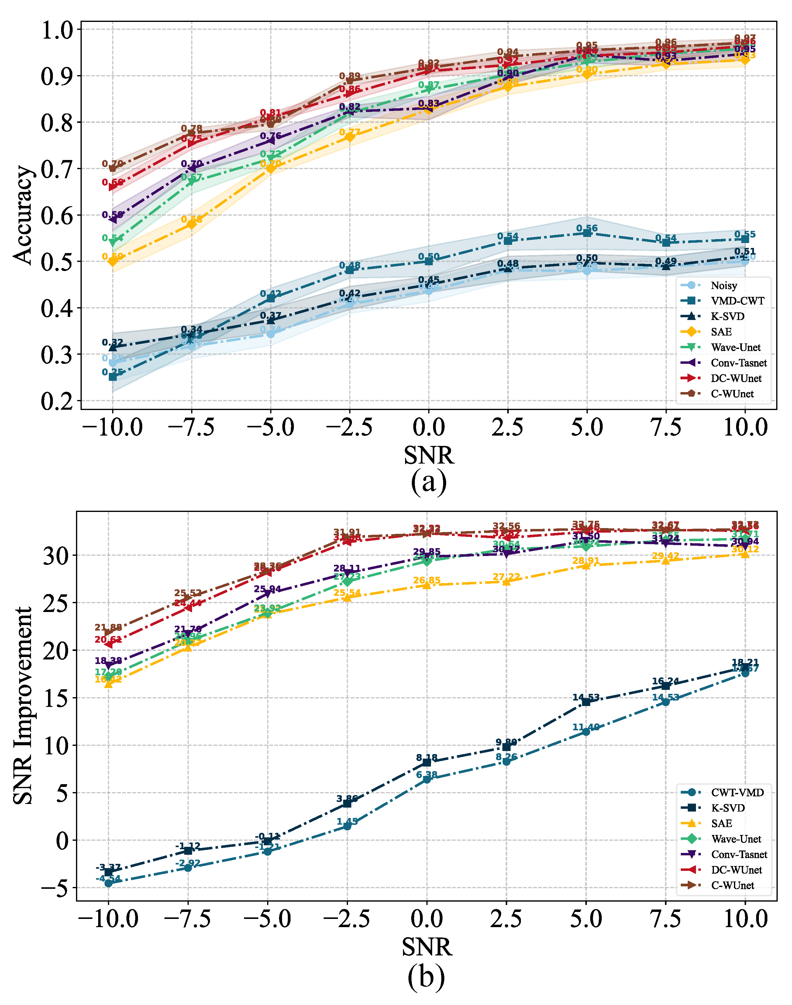
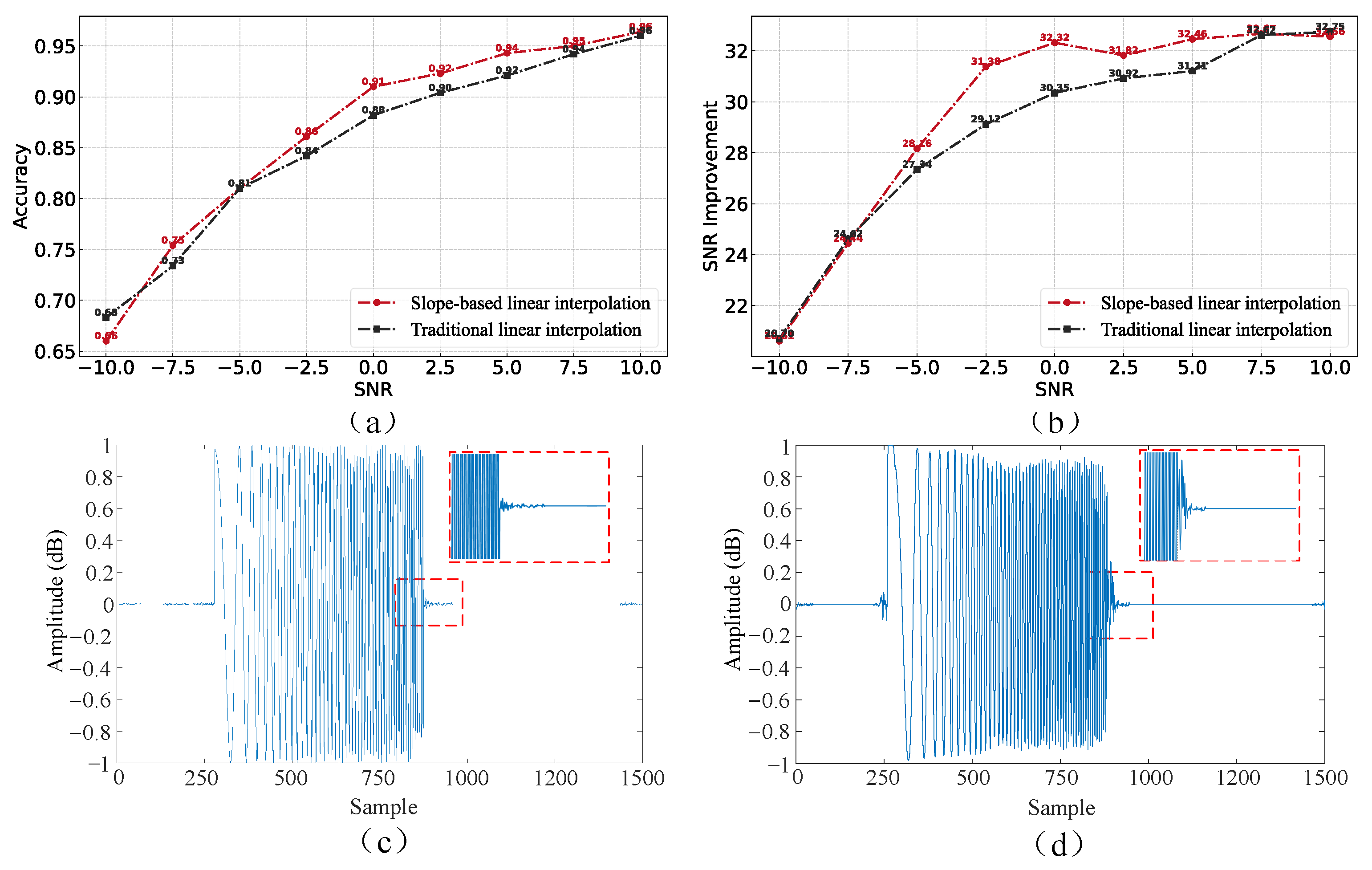
6.2. Comparison of TOA Accuracy and SNR Improvement
Table 3 and Table 4 and Figure 10 present the experimental results under nine SNR conditions with ship-radiated noise and multipath Doppler interference. The results show that DC-WUnet outperforms SAE, Wave-Unet, and Conv-Tasnet in terms of both delay estimation accuracy and SNR improvement. Under low SNR conditions, DC-WUnet leverages the powerful feature extraction capabilities of the Conformer module to effectively capture target signals obscured by noise. As a result, it achieves significantly improved delay estimation accuracy and output SNR compared to baseline algorithms. Notably, when the SNR drops to an extremely low level of −10 dB, the proposed method still maintains robust performance. It achieves at least a 32% improvement in delay estimation accuracy and a 2.3 dB gain in output SNR, relative to other competing methods. Under high SNR conditions, DC-WUnet relies on multiscale features extracted through skip connections to achieve higher accuracy in signal reconstruction. Since the noise interference is smaller in high SNR conditions, all deep learning algorithms perform better, and the improvement over other algorithms is relatively small.
Table 3.
Under nine different SNR conditions, various signal enhancement algorithms were applied to interference signals to estimate the TOA. The estimated TOAs were then compared with the ground truth values to evaluate the accuracy of time delay estimation. The detailed methodology is provided in Section 5.3.
Table 4.
Under nine different SNR conditions, various signal enhancement algorithms were applied to interference-contaminated signals. The SNR of the enhanced signals was estimated and compared with that of the original interference signals to evaluate the SNR improvement. The detailed calculation method is provided in Section 5.3.
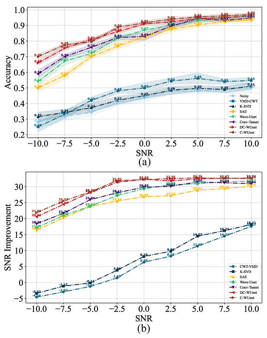
Figure 10.
Performance of seven methods versus SNR with ship-radiated noise; (a) TOA accuracy, where Noisy denotes the received hydroacoustic signal without processing, and the shaded area represents the standard deviation of the three-fold cross-validation; (b) SNR improvement.
The shaded region in Figure 10 represents the error range after three-fold cross-validation. The results show that DC-WUnet and C-WUnet have smaller error ranges, indicating stronger robustness. Both models incorporate the Conformer module, which uses multi-head attention to extract key information from different feature spaces, thus enhancing model robustness. Additionally, both DC-WUnet and C-WUnet employ joint time–frequency domain training, which imposes stricter constraints on signal reconstruction, further improving their robustness.
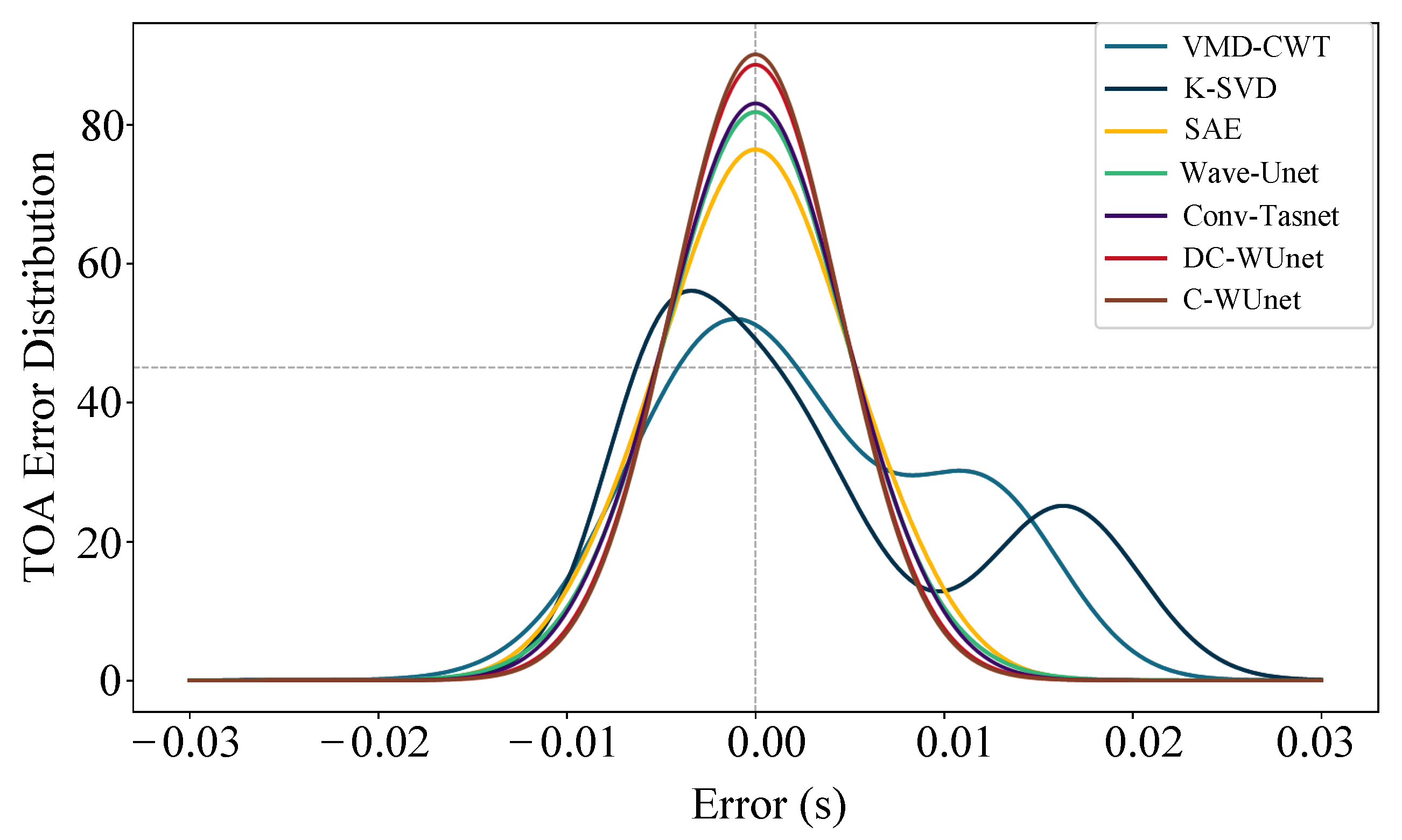
Figure 11 presents the TOA estimation error distributions. The results show that the error distribution curves of both C-WUnet and DC-WUnet are higher and narrower compared to those of other algorithms. This indicates that their estimation errors are more tightly concentrated around zero, reflecting smaller average errors. In the context of underwater localization, such reduced delay estimation errors translate directly into lower positioning errors. These findings suggest that C-WUnet and DC-WUnet are better suited for reliable signal processing in underwater localization tasks. The traditional time–frequency domain algorithms KSVD and VMD-CWT can improve noise reduction and increase the SNR to some extent. However, in low SNR conditions, they lack the ability to effectively capture and reconstruct the signal, resulting in substantial residual noise and low TOA accuracy. In high SNR conditions, noise is no longer the primary factor affecting TOA accuracy. Instead, signal superposition and frequency shifts caused by multipath and Doppler effects severely impact TOA estimation accuracy, leading to large positioning errors. Therefore, these algorithms are not suitable for use in underwater acoustic signal positioning systems.
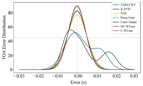
Figure 11.
TOA error distributions for seven methods.
6.3. Different Interpolation Methods Performance
According to Figure 12a,b, it can be seen that the slope-weighted interpolation method improves the correct TOA rate and signal-to-noise ratio over the traditional interpolation method under high SNR conditions, whereas it is not much different from the traditional interpolation method under low SNR conditions. This is because at high SNR, the noise component in the signal is smaller, and the slope more accurately reflects the trend of the data. The interpolation method based on slope weighting can make better use of the neighborhood data information before and after the target signal, which can make the interpolation point closer to the real signal, inhibit the high-frequency noise introduced before and after the target signal, and enhance the effect better than linear interpolation. As shown in Figure 12c,d., under the condition of a low signal-to-noise ratio, the noise component in the signal is significant, the slope calculation may be affected by noise, and the enhancement effect is similar to linear interpolation.
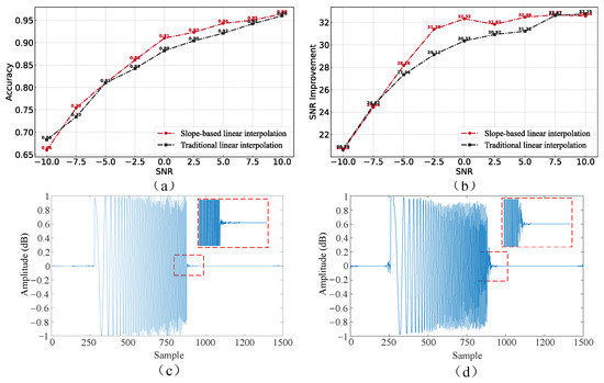
Figure 12.
(a,b) DC-WUnet network enhancement based on two different interpolation methods, respectively. (c,d) Show the performance of DC-WUnet based on slope interpolation and traditional interpolation, respectively, at SNR = −2.5 dB.
6.4. DC-WUnet Performance
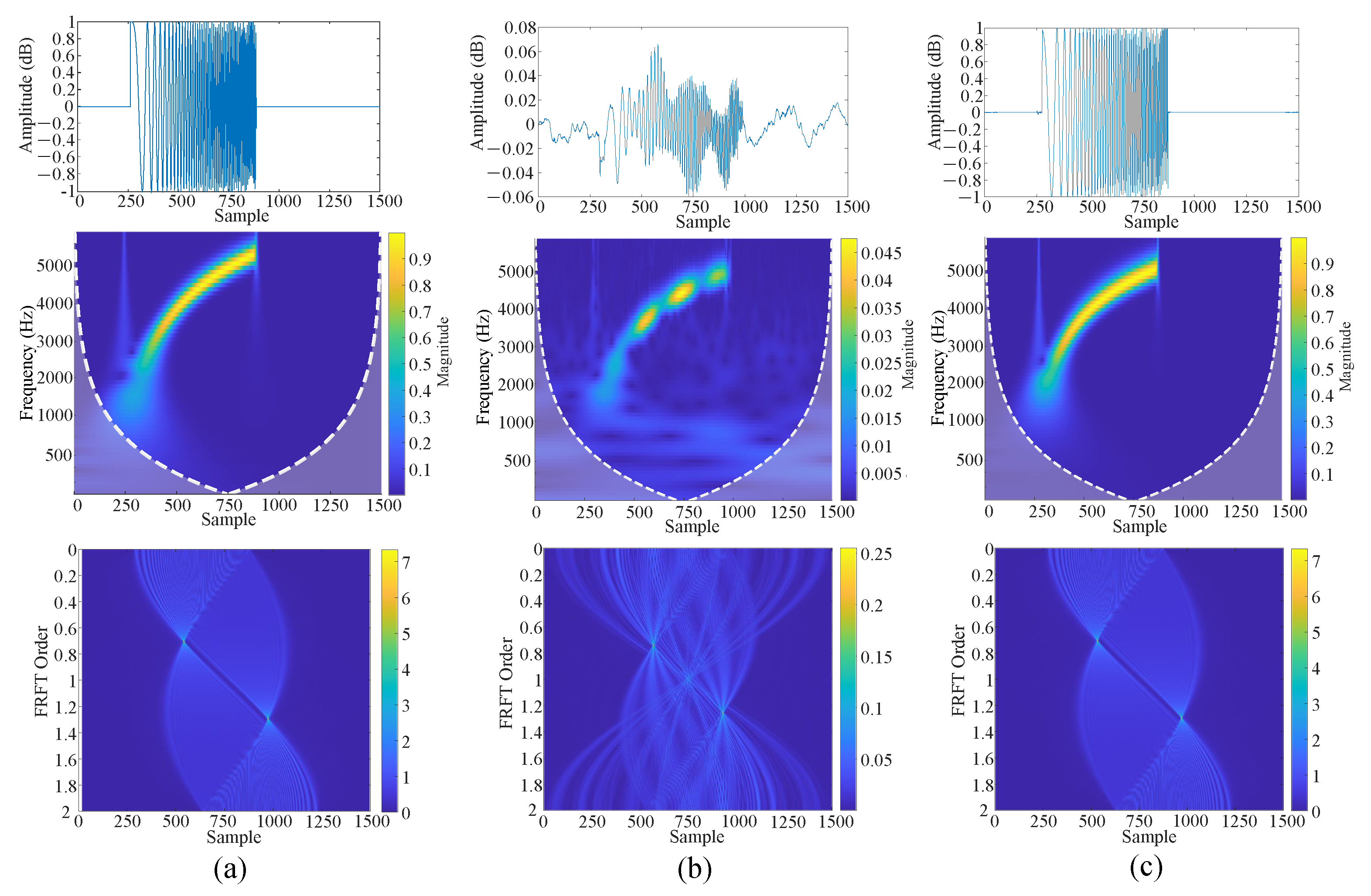
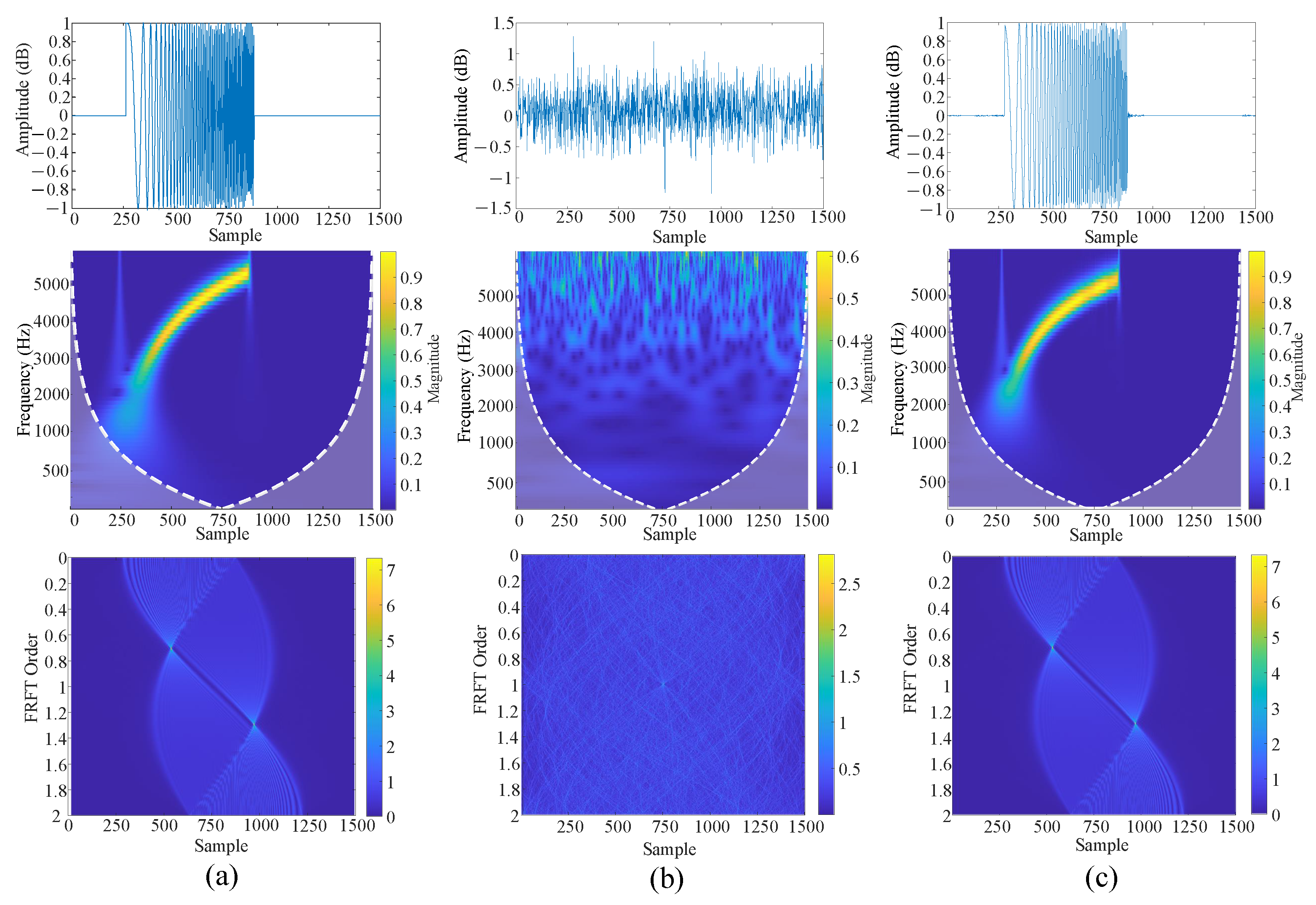
Figure 13b and Figure 14b present the interfering signal at SNR = 2.5 dB and −2.5 db in the time domain, frequency domain, and 2D Fractional Fourier Transform (FRFT), respectively. The corresponding results after DC-WUnet processing are given in Figure 13c and Figure 14c. The clean signal results are shown in Figure 13a and Figure 14a.
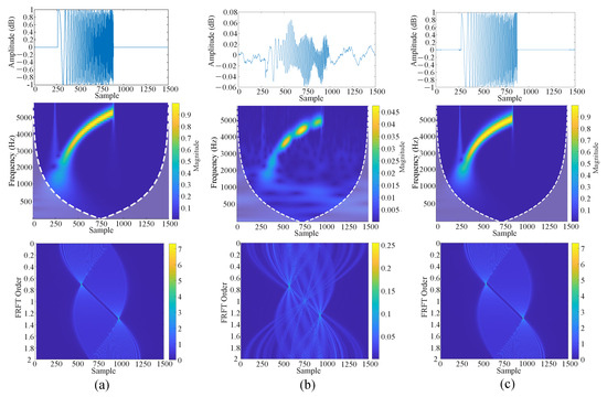
Figure 13.
DC-WUnet performance improvement at SNR = 2.5 dB. (a) The clean signal; (b) the interfering signal to be enhanced; (c) the signal obtained after DC-WUnet enhancement.
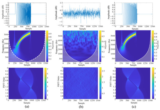
Figure 14.
DC-WUnet performance improvement at SNR = −2.5 db. (a) The clean signal; (b) the interfering signal to be enhanced; (c) the signal obtained after DC-WUnet enhancement.
By comparing the time-domain representations, it is evident that the proposed method effectively reconstructs the target waveform while successfully suppressing the noise components.
In the frequency domain, the method demonstrates a strong ability to restore the distortions caused by Doppler effects, yielding a frequency profile that closely resembles that of the clean signal. Furthermore, the two-dimensional Fractional Fourier Transform (FRFT) results reveal that the original signal is severely affected by multipath interference, characterized by distorted and sparsely distributed search lines. In contrast, the enhanced signal obtained using the proposed method exhibits significantly clearer and denser search lines. These results collectively indicate that the proposed method effectively mitigates time-frequency distortions caused by multipath propagation and Doppler shifts, thereby contributing to improved accuracy in identifying and localizing acoustic signals in underwater positioning systems.
6.5. Network Parameter and Execution Time Comparison
Table 5 presents the number of parameters, execution time, and FLOPs (floating-point operations). The results indicate that C-WUnet, due to the addition of the Conformer module, experiences an increase in the number of parameters, leading to higher processing time and computational load. This can potentially cause memory overflow and excessive runtime in resource-constrained applications with slower CPUs. In contrast, DC-WUnet employs depthwise separable convolutions, where each input channel is convolved independently, followed by pointwise convolutions to combine the outputs across channels. This reduces computational cost, requires fewer parameters, and enables faster execution. Additionally, compared to other algorithms, DC-WUnet is more lightweight in terms of parameter count, runtime, and FLOPs.
Table 5.
Comparison of computational efficiency and model complexity of various deep learning algorithms. Smaller parameter counts, faster inference, and lower FLOPs indicate lower memory and computational demands, favoring deployment in resource-constrained environments.
7. Conclusions
This paper addresses the significant issue of positioning accuracy degradation for ranging signals caused by ship-radiated noise and multipath Doppler interference. It introduces DC-WUnet, a time-domain acoustic signal enhancement deep learning framework based on a codec structure. It solves problems such as inaccurate TOA and low SNR caused by ship-radiated noise and multipath Doppler effects.
DC-WUnet utilizes a U-shaped convolutional network (U-Net) architecture for signal enhancement. In the encoding layer, a Conformer module and skip connections are introduced to enhance the network’s ability to capture the target signal’s features while providing multiscale features to the decoding layer for target signal reconstruction. In the decoding layer, slope-based linear interpolation is employed to ensure the continuity of signal features, better align with the target signal’s trend, and suppress noise. Our evaluation results show that DC-WUnet outperforms other systems, even under low SNR conditions. Furthermore, DC-WUnet adopts depthwise-separable convolutions, which reduce model parameters and computation time, making it highly suitable for low-resource, low-latency applications such as underwater vehicles.
However, although DC-WUnet performs excellently in simulated environments, it still faces several challenges in real-world underwater applications. For example, the underwater acoustic environment, in reality, is more complex and may contain additional unknown noise sources and interference signals, which could affect the model’s robustness and accuracy. On the other hand, the model’s computational efficiency still needs further optimization in resource-constrained scenarios to meet the requirements for real-time performance and low latency.
Therefore, future research will include field testing based on underwater positioning devices to further evaluate the performance of DC-WUnet in real-world underwater environments. Additionally, we plan to optimize the model’s computational efficiency and generalization ability, exploring its application in more complex environments to enhance the model’s adaptability and stability in practical applications.
Author Contributions
Conceptualization, X.L. and J.L.; formal analysis, X.L. and J.Z.; funding acquisition, J.L.; methodology, X.L.; software, X.L. and Y.B.; supervision, X.L. and J.L.; validation, X.L. and J.Z.; writing—original draft, X.L.; writing—review and editing, X.L., Y.B. and Z.C. All authors have read and agreed to the published version of the manuscript.
Funding
This work was supported by the National Natural Science Foundation of China No. 62231028.
Data Availability Statement
The original contributions presented in this study are included in the article. Further inquiries can be directed to the corresponding author.
Conflicts of Interest
The authors declare no conflicts of interest.
References
- Reis, J.; Morgado, M.; Batista, P.; Oliveira, P.; Silvestre, C. Design and experimental validation of a usbl underwater acoustic positioning system. Sensors 2016, 16, 1491. [Google Scholar] [CrossRef] [PubMed]
- Kim, J. Hybrid toa–doa techniques for maneuvering underwater target tracking using the sensor nodes on the sea surface. Ocean Eng. 2021, 42, 110110. [Google Scholar] [CrossRef]
- Zhang, B.; Xiang, Y.; He, P.; Zhang, G.-j. Study on prediction methods and characteristics of ship underwater radiated noise within full frequency. Ocean Eng. 2019, 174, 61–70. [Google Scholar] [CrossRef]
- Smith, T.A.; Rigby, J. Underwater radiated noise from marine vessels: A review of noise reduction methods and technology. Ocean Eng. 2022, 266, 112863. [Google Scholar] [CrossRef]
- Tan, H.-P.; Diamant, R.; Seah, W.K.; Waldmeyer, M. A survey of techniques and challenges in underwater localization. Ocean Eng. 2011, 38, 1663–1676. [Google Scholar] [CrossRef]
- Rioul, O.; Duhamel, P. Fast algorithms for discrete and continuous wavelet transforms. IEEE Trans. Inf. Theory 1992, 38, 569–586. [Google Scholar] [CrossRef]
- Hariharan, S.M.; Kamal, S.; Pillai, S. Reduction of self-noise effects in onboard acoustic receivers of vessels using spectral subtraction. In Proceedings of the Acoustics 2012 Nantes Conference, Nantes, France, 23–27 April 2012. [Google Scholar]
- Czapiewska, A.; Luksza, A.; Studanski, R.; Zak, A. Reduction of the multipath propagation effect in a hydroacoustic channel using filtration in cepstrum. Sensors 2020, 20, 751. [Google Scholar] [CrossRef]
- Liu, Y.; Zhou, W.; Li, P.; Yang, S.; Tian, Y. An ultrahigh frequency partial discharge signal de-noising method based on a generalized s-transform and module time-frequency matrix. Sensors 2016, 16, 941. [Google Scholar] [CrossRef]
- Dragomiretskiy, K.; Zosso, D. Variational mode decomposition. IEEE Trans. Signal Process. 2013, 62, 531–544. [Google Scholar] [CrossRef]
- Aharon, M.; Elad, M.; Bruckstein, A. K-svd: An algorithm for designing overcomplete dictionaries for sparse representation. IEEE Trans. Signal Process. 2006, 54, 4311–4322. [Google Scholar] [CrossRef]
- Yang, W.; Peng, Z.; Wei, K.; Shi, P.; Tian, W. Superiorities of variational mode decomposition over empirical mode decomposition particularly in time–frequency feature extraction and wind turbine condition monitoring. IET Renew. Power Gener. 2017, 11, 443–452. [Google Scholar] [CrossRef]
- Fu, S.-W.; Tsao, Y.; Lu, X.; Kawai, H. Raw waveform-based speech enhancement by fully convolutional networks. In Proceedings of the 2017 Asia-Pacific Signal and Information Processing Association Annual Summit and Conference (APSIPA ASC), Kuala Lumpur, Malaysia, 12–15 December 2017; pp. 6–12. [Google Scholar] [CrossRef]
- Wang, H.; Wu, X.; Huang, Z.; Xing, E.P. High-frequency component helps explain the generalization of convolutional neural networks. In Proceedings of the IEEE/CVF Conference on Computer Vision and Pattern Recognition, Seattle, WA, USA, 13–19 June 2020; pp. 8684–8694. [Google Scholar]
- Yang, S.; Xue, L.; Hong, X.; Zeng, X. A lightweight network model based on an attention mechanism for ship-radiated noise classification. J. Mar. Sci. Eng. 2023, 11, 432. [Google Scholar] [CrossRef]
- Kumar Pc, K.; Palani, S.; Selvaraj, J.; Rajendran, V. De-noising algorithm for snr improvement of underwater acoustic signals using cwt based on fourier transform. Underw. Technol. 2018, 35, 23–30. [Google Scholar] [CrossRef]
- Barbarossa, S. Analysis of multicomponent lfm signals by a combined wigner-hough transform. IEEE Trans. Signal Process. 1995, 43, 1511–1515. [Google Scholar] [CrossRef]
- Dai, Y.; Xue, Y.; Zhang, J. A continuous wavelet transform approach for harmonic parameters estimation in the presence of impulsive noise. J. Sound Vib. 2016, 360, 300–314. [Google Scholar] [CrossRef]
- Li, S.; Zhao, J.; Wu, Y.; Bian, S.; Zhai, G. Prior frequency information assisted vmd method for sbp sonar data noise removal. IEEE Geosci. Remote Sens. Lett. 2023, 20, 7503905. [Google Scholar] [CrossRef]
- Xiao, F.; Yang, D.; Guo, X.; Wang, Y. Vmd-based denoising methods for surface electromyography signals. J. Neural Eng. 2019, 16, 056017. [Google Scholar] [CrossRef]
- Donoho, D.L. De-noising by soft-thresholding. IEEE Trans. Inf. Theory 1995, 41, 613–627. [Google Scholar] [CrossRef]
- Yang, H.; Li, L.; Li, G. A new denoising method for underwater acoustic signal. IEEE Access 2020, 8, 201874–201888. [Google Scholar] [CrossRef]
- Wu, Y.; Xing, C.; Zhang, D.; Xie, L. Low-frequency underwater acoustic signal denoising method in the shallow sea with a low signal-to-noise ratio. In Proceedings of the 2021 OES China Ocean Acoustics (COA), Harbin, China, 14–17 July 2021; pp. 731–735. [Google Scholar] [CrossRef]
- Ahmed, N.; Natarajan, T.; Rao, K.R. Discrete cosine transform. IEEE Trans. Comput. 1974, 100, 90–93. [Google Scholar] [CrossRef]
- Rubinstein, R.; Zibulevsky, M.; Elad, M. Efficient Implementation of the k-Svd Algorithm Using Batch Orthogonal Matching Pursuit. CS Technion Technical Report. 2008. Available online: https://www.researchgate.net/publication/251229200_Efficient_Implementation_of_the_K-SVD_Algorithm_Using_Batch_Orthogonal_Matching_Pursuit (accessed on 22 March 2025).
- Gogna, A.; Majumdar, A.; Ward, R. Semi-supervised stacked label consistent autoencoder for reconstruction and analysis of biomedical signals. IEEE Trans. Biomed. Eng. 2016, 64, 2196–2205. [Google Scholar] [CrossRef] [PubMed]
- Wang, X.; Zhao, Y.; Teng, X.; Sun, W. A stacked convolutional sparse denoising autoencoder model for underwater heterogeneous information data. Appl. Acoust. 2020, 167, 107391. [Google Scholar] [CrossRef]
- Russo, P.; Ciaccio, F.D.; Troisi, S. Danae++: A smart approach for denoising underwater attitude estimation. Sensors 2021, 21, 1526. [Google Scholar] [CrossRef]
- Guimarães, H.R.; Nagano, H.; Silva, D.W. Monaural speech enhancement through deep wave-u-net. Expert Syst. Appl. 2020, 158, 113582. [Google Scholar] [CrossRef]
- Macartney, C.; Weyde, T. Improved speech enhancement with the wave-u-net. arXiv 2018, arXiv:1811.11307. [Google Scholar]
- Chu, H.; Li, C.; Wang, H.; Wang, J.; Tai, Y.; Zhang, Y.; Yang, F.; Benezeth, Y. A deep-learning based high-gain method for underwater acoustic signal detection in intensity fluctuation environments. Appl. Acoust. 2023, 211, 109513. [Google Scholar] [CrossRef]
- Luo, Y.; Mesgarani, N. Conv-tasnet: Surpassing ideal time–frequency magnitude masking for speech separation. IEEE/ACM Trans. Audio Speech Lang. Process. 2019, 27, 1256–1266. [Google Scholar] [CrossRef]
- Irfan, M.; Jiangbin, Z.; Ali, S.; Iqbal, M.; Masood, Z.; Hamid, U. Deepship: An underwater acoustic benchmark dataset and a separable convolution based autoencoder for classification. Expert Syst. Appl. 2021, 183, 115270. [Google Scholar] [CrossRef]
- Gul, S.; Zaidi, S.S.H.; Khan, R.; Wala, A.B. Underwater acoustic channel modeling using bellhop ray tracing method. In Proceedings of the 2017 14th International Bhurban Conference on Applied Sciences and Technology (IBCAST), Islamabad, Pakistan, 10–14 January 2017; pp. 665–670. [Google Scholar] [CrossRef]
- Kuniyoshi, S.; Oshiro, S.; Saotome, R.; Wada, T. An iterative orthogonal frequency division multiplexing receiver with sequential inter-carrier interference canceling modified delay and doppler profiler for an underwater multipath channel. J. Mar. Sci. Eng. 2024, 12, 1712. [Google Scholar] [CrossRef]
- Neipp, C.; Hernández, A.; Rodes, J.; Márquez, A.; Beléndez, T.; Beléndez, A. An analysis of the classical doppler effect. Eur. J. Phys. 2003, 24, 497. [Google Scholar] [CrossRef]
- Li, B.; Zhou, S.; Stojanovic, M.; Freitag, L.; Willett, P. Multicarrier communication over underwater acoustic channels with nonuniform doppler shifts. IEEE J. Ocean Eng. 2008, 33, 198–209. [Google Scholar] [CrossRef]
- Qu, F.; Wang, Z.; Yang, L.; Wu, Z. A journey toward modeling and resolving doppler in underwater acoustic communications. IEEE Commun. Mag. 2016, 54, 49–55. [Google Scholar] [CrossRef]
- Abdelkareem, A.E.; Sharif, B.S.; Tsimenidis, C.C. Adaptive time varying doppler shift compensation algorithm for ofdm-based underwater acoustic communication systems. Ad Hoc Netw. 2016, 45, 104–119. [Google Scholar] [CrossRef]
- Tanaka, S.; Nomura, H.; Kamakura, T. Doppler shift equation and measurement errors affected by spatial variation of the speed of sound in sea water. Ultrasonics 2019, 94, 65–73. [Google Scholar] [CrossRef]
- Porter, M.B. The Bellhop Manual and User’s Guide: Preliminary Draft; Heat, Light, and Sound Research, Inc.: La Jolla, CA, USA, 2011; Volume 260. [Google Scholar]
- Gulati, A.; Qin, J.; Chiu, C.-C.; Parmar, N.; Zhang, Y.; Yu, J.; Han, W.; Wang, S.; Zhang, Z.; Wu, Y.; et al. Conformer: Convolution-augmented transformer for speech recognition. arXiv 2020, arXiv:2005.08100. [Google Scholar]
- Ramachandran, P.; Zoph, B.; Le, Q.V. Swish: A self-gated activation function. arXiv 2017, arXiv:1710.05941; Volume 7, p. 5. [Google Scholar]
- Bridle, J. Training Stochastic Model Recognition Algorithms as Networks Can Lead to Maximum Mutual Information Estimation of Parameters. Available online: https://proceedings.neurips.cc/paper_files/paper/1989/file/0336dcbab05b9d5ad24f4333c7658a0e-Paper.pdf (accessed on 22 March 2025).
- Dauphin, Y.N.; Fan, A.; Auli, M.; Grangier, D. Language modeling with gated convolutional networks. In Proceedings of the International Conference on Machine Learning, PMLR, Sydney, NSW, Australia, 6–11 August 2017; pp. 933–941. [Google Scholar]
- Ioffe, S.; Szegedy, C. Batch normalization: Accelerating deep network training by reducing internal covariate shift. In Proceedings of the International Conference on Machine Learning, PMLR, Lille, France, 6–11 July 2015; pp. 448–456. [Google Scholar]
- Kingma, D.P.; Ba, J. Adam: A method for stochastic optimization. arXiv 2014, arXiv:1412.6980. [Google Scholar]


Disclaimer/Publisher’s Note: The statements, opinions and data contained in all publications are solely those of the individual author(s) and contributor(s) and not of MDPI and/or the editor(s). MDPI and/or the editor(s) disclaim responsibility for any injury to people or property resulting from any ideas, methods, instructions or products referred to in the content. |
© 2025 by the authors. Licensee MDPI, Basel, Switzerland. This article is an open access article distributed under the terms and conditions of the Creative Commons Attribution (CC BY) license (https://creativecommons.org/licenses/by/4.0/).