Wavy Wind-Water Flow Impacts on Offshore Wind Turbine Foundations

Abstract

The present study investigates the flow dynamics surrounding offshore wind turbine OWT foundations, focusing on the interaction of wind and water flows with two prevalent foundation types: mono-pile and tripod designs. Computational simulations and analyses were conducted on the substructures of these OWTs using the ANSYS-Fluent v16.5 software package. The primary objective was to predict critical parameters, including directional drag force coefficients, interface velocities, and pressure distributions. To model realistic oceanic conditions, pseudo-periodic wave patterns were implemented at the inlet boundary. The flow regime was characterized by logarithmic vertical velocity profiles at low interfacial velocities, ranging from 2.23 m/s to 3.01 m/s. This computational approach revealed anisotropic constraints imposed on the foundations under unidirectional flow conditions. The drag coefficients obtained from the simulations highlighted significant vertical flux exchanges in proximity to the OWT structures, with a particularly pronounced downward flow near the tripod foundation design. Additionally, the study demonstrated that variations in wind speed within the specified range did not substantially impact pressure distributions or strain rates. However, these changes were found to influence skin friction coefficients, indicating a sensitivity of these hydrodynamic parameters to wind speed variations. The analysis of flow streamlines around the mono-pile foundation showed a smooth and well-defined pattern, whereas the flow around the tripod foundation exhibited more complex, interleaved, and turbulent streamlines. This distinction in flow behavior is believed to contribute to the observed downward vertical flux exchanges near the tripod.

1. Introduction

The growing demand for renewable energy has significantly driven the expansion of the wind energy sector. Offshore wind turbines OWTs represent a particularly promising solution, primarily due to the availability of higher and more consistent wind speeds offshore compared to onshore locations, as well as the abundance of vast, uninhabited areas suitable for development. Moreover, the emerging potential for electrolysis-based green hydrogen production from seawater positions offshore wind-to-hydrogen technologies as a key transformative component of the renewable energy landscape. However, the installation of offshore wind turbines is associated with substantial costs and presents additional engineering challenges, particularly in relation to the geological properties of seabed soils and the dynamic environmental conditions encountered offshore. These conditions, which include high wave loading, large structural strains, and extreme weather, necessitate comprehensive and detailed structural assessments. Research has shown that offshore wind turbines can generate up to 50% more electricity than their onshore counterparts [1]. Despite this potential, it is critical to ensure that the design and engineering of offshore wind turbine towers are robust enough to withstand extreme weather events and mechanical stresses. In onshore settings, wind gusts are a primary consideration, while in offshore environments, wave forces and oceanic conditions, including wave power, play a dominant role in determining turbine performance. The mechanical energy input from wind to the ocean drives ocean currents, enhances surface waves, and induces turbulence and mixing, all of which influence the operational environment of offshore turbines. A global estimate of wind-ocean kinetic energy flux, as reported in [2], suggests a total energy flow of approximately 70 terawatts, highlighting the immense potential of offshore wind energy in the global energy mix.

In the context of marine structures, wave and current forces account for more than 70% of the environmental factors influencing the dynamic response of substructures [3]. The impact of waves is inherently linked to wind effects, and recent studies [4] have demonstrated that the coupling between wind and current stresses significantly enhances wind-sea energy exchanges. The design and construction of foundations for offshore wind turbines are critical to ensuring the long-term sustainability and performance of these installations, particularly in terms of their ability to withstand cyclic loading and maintain optimal natural frequencies. According to [5], installation costs represent approximately 60% of the total expenditure associated with offshore wind farm development. Offshore wind turbine foundations are subjected to various environmental forces, including wind, hydrodynamic wave action, and in some regions, ice. These forces can exert substantial side loads and bending moments on the foundations, while vertical loads are comparatively less significant. The design of OWT foundations must therefore account for these complex and dynamic loading conditions. Additionally, foundation designs are influenced by a range of factors, including the characteristics of the seabed geology, water depth, and the history of currents in the region. These constraints necessitate a tailored approach to foundation design, ensuring that each installation can effectively respond to the specific environmental conditions of its site.

An efficient and accurate numerical model for predicting the dynamic response of offshore wind turbines to coupled environmental loads is essential for robust design and operational performance. Among the well-established simulation tools, FAST and MSC.ADAMS stand out as comprehensive aero-servo-elastic simulators, developed at the National Renewable Energy Laboratory NREL and the National Wind Technology Center NWTC, respectively. In series of researches conducted in [6,7] performed simulations with OpenFoam CFD of a fully coupled aero-hydro-mooring of the NREL 5 MW OC4 semi-submersible Floating Offshore Wind Turbine FOWT with accurate validation against existing experiments and numerical data. The research also highlighted the importance of each component in the aero-hydro-mooring system. These packages are capable of providing realistic predictions of FOWT performance under various environmental conditions. The impact of wave forces and run-up on OWTs and other marine structures has been the subject of significant research. For example, ref. [8] observed that larger waves tend to break as they approach foundations, with the breaking process significantly influencing both the wave run-up and the wave pressures. Further studies, such as [9], have explored the effects of breaking waves on mono-pile foundations using computational fluid dynamics CFD models, reporting that peak forces associated with plunging breakers decrease during the breaking process. The assessment of wave-induced stresses on single pile foundations for wind turbines, conducted by [8], found that for small waves, results from CFD simulations closely align with predictions based on the Morison equation using the stream function approach. The structural characteristics of mono-pile and tripod foundations were studied by [10] using the ANSYS software package in both static and modal simulations. Their findings indicated that the mono-pile design has a shorter expected lifespan compared to the tripod, and that the magnitudes of maximum stresses and natural frequencies significantly differ between the two foundation types. Moreover, the tripod design exhibited superior stiffness and better stress-control capabilities, making it a more resilient choice for offshore wind turbine installations. In addition, investigations into unsteady fluid flows around different foundation types, such as mono-pile, tripod, and jacket structures, were conducted by [11] using ANSYS-CFX in the time domain. Their study revealed similar rotor forces for the jacket and tripod designs, though the projected hydrodynamic load was lower for the jacket foundation compared to the mono-pile and tripod.

The interaction between the atmosphere and ocean forms a coupled subsystem, with dynamic exchanges occurring at the air-sea interface. These exchanges involve the transfer of constituents, turbulence, and heat fluxes between the atmosphere and ocean, with the intensity of these interactions being highly dependent on prevailing meteorological conditions. During severe weather events, the boundary between the sea and the atmosphere may become indistinct, further complicating the modeling of wind-sea exchanges. The challenges in accurately simulating these exchanges arise from the complexity of the governing physical processes, their inter-dependencies, and the unsteady, spatio-temporal nature of the phenomena involved. Key questions regarding the processes of energy, momentum, and constituent transfer at the wind-sea interface remain only partially understood. Early laboratory experiments, such as those conducted by [12], provided valuable data on wind-wave interactions and helped advance the understanding of wave forcing and excitation. Later, more advanced experimental studies, including those reported by [13,14,15,16], and provided detailed data on specific inflow properties and conditions, albeit within limited parameter ranges. On the other hand, numerous field campaigns, as documented in [2,17,18], have yielded valuable insights into the wind-sea interactions. Other field studies have focused on the effects of swell waves on air-sea wind stress [19,20]. While progress has been made in understanding wind-sea-swell interactions, the outcomes of these studies remain specific and not fully generalizable, limiting their applicability for broader adaptation in offshore wind turbine design. Significant advancements have been made in numerical modeling techniques for wind-wave coupling, particularly through methods such as Direct Numerical Simulation DNS [21,22,23] and Large-Eddy Simulation LES [24,25,26]. These approaches have provided detailed insights into wave-induced perturbations and stresses, the impact of surface waves on boundary layers, and the associated mixing processes—knowledge that is difficult to obtain through direct observational methods.

Various approaches have been developed to model wind-wave interactions within numerical simulations. One such method involves considering the air pressure distribution over the wave surface [27,28]. This approach facilitates the modelling of wave growth and propagation, allowing for a more realistic representation of the air-sea interface. However, its application is primarily limited to potential water flow scenarios, as its validation is constrained to idealized conditions that may not fully capture the complexities of real-world wave dynamics. The fully coupled wind-wave model presented in [29] investigates the dynamics of wind-wave interactions through a fully coupled two-phase flow framework. The model simulates a scenario where wind flows over a moving wavy water surface, influencing the atmospheric boundary layer (ABL) and inducing surface wind stress that in turn transfers energy to the waves. The authors documented the intricate evolution of the coupled wind-wave system, observing significant changes in wave amplitude and shape, the development of underwater drift currents, and the feedback effects on the air-side turbulent boundary layer. A more recent study by [30] also delves into the wind-wave interaction mechanisms, employing a volume of fluid VOF method to solve the dynamics of the two-phase flow. In this approach, the wind’s Reynolds number is treated as the primary governing parameter. The flow setup involves the imposition of a constant pressure gradient in the streamwise direction, thereby establishing friction velocities for both the wind and water boundary layers. However, by restricting the study to constant pressure gradients, the analysis is confined to periodic solutions within the flow system. The approach presented in [31] integrated a data-driven framework with CFD using the Volume of Fluid VOF method and statistical techniques, coupled with active sampling of training data, to investigate the behavior of a mono-pile foundation under hydrodynamic loads. The initial setup included a fixed inlet velocity and a superposition of linear regular wave components. In a similar context, the study in [32] explored free-surface channel flow around a square cylinder using a VOF model. This study involved uniform velocity with prescribed Froude ${\mathcal{F}}_r$ and Reynolds ${\mathcal{R}}_e$ numbers, with a focus on analyzing the flow state both upstream and downstream of the cylinder. The authors identified a range of flow regimes, including subcritical, choked, and supercritical states, based on the variations of the Froude number.

Despite its fundamental importance in offshore environments, wind-sea interaction has not been fully integrated into the design process for OWTs. International standards for OWTs were only established in 2009. Existing literature on aero-hydrodynamic loads on OWTs, to the best of our knowledge, has primarily focused on uniform wind conditions and has not considered the coupling between wind and sea dynamics using vertical wind-sea velocity profiles.

This work aims at to address this gap by illustrating wind-sea coupling through logarithmic vertical velocity profiles, implemented using user-defined functions UDFs to investigate the aero-hydrodynamic loads on OWT foundations. In addition to the vertical profiles, a superposition of permanent inlet waves is introduced to complete the initial setup. The present methodology builds on the framework developed by Chen and Zou in [33], which primarily focused on analyzing the effects of vertical current shear on nonlinear wave interactions. To address the wind-sea interaction effects on OWT foundations, we adopt the logarithmic law for vertical wind-water velocity profiles, which is grounded in Monin-Obukhov MO similarity theory that assumes a constant turbulent fluxes with altitude and the homogeneous character of a horizontal surrounding surface. Although the limitations of MO similarity theory were demonstrated in various studies; as in [34,35], it is taking as a starting point in this work. The accuracy of these vertical velocity profiles is crucial, as they govern sea surface roughness, influence the dynamics of the adjacent boundary layers, and affect heat recirculation. Under such profiles, OWT structures experience negative stresses, particularly in regions with negative gradients, which are often observed in atmospheric velocity profiles. Some OWT foundations, located in areas where waves propagate under the influence of currents or wind, experience significant wave-current or wave-wind interactions. The drag and lift forces exerted on these foundations are proportional to the square of the entrained seawater velocity. The entrainment coefficient plays a critical role in determining the amount of water displaced towards the foundation. Depending on the design conditions, both drag and lift forces may dominate over inertia forces. In regions with strong winds, wave-current interactions are common, leading to altered wave behavior and generating unpredictable hydrodynamic loads on the OWT foundations.

The primary objective of this study is to investigate the effects of wind-sea flows on OWT foundations. For this purpose, piecewise logarithmic wind-water vertical velocity profiles were considered, parametrized for low interfacial speeds in the range of 2.0 m/s $\le U_{ws}\le$ 3.01 m/s around mono-pile and tripod foundations. In this study, the offshore foundations are treated as isolated entities, independent of the wind turbines themselves, in order to isolate and assess the effects of wind and water alone. This approach also allows for the modeling of downsized problems in terms of meshing and computational complexity. The simulations were performed using the VOF model in ANSYS-Fluent, with a primary focus on estimating the aero-hydrodynamic loads on the foundations. The hydrodynamic behavior around the foundations is examined through various parameters, including path lines, air-water velocity distributions, and dynamic pressures. The introduction of a vertical current profile coupled with waves is expected to alter the flow characteristics, including the magnitudes and profiles of the hydrodynamic loads. Additionally, directional drag coefficients are computed for both the mono-pile and tripod foundation types. An attempt is also made to reformulate the dynamic Froude ${\mathcal{F}}_r$ in terms of kinetic energy (dynamic pressure) and potential energy (mixing efficiency). This reformulation aims to establish a relationship between the Froude number, wind kinetic energy transfer, and wind stress.

The structure of this work is as follows: Section 2 outlines the mathematical model used for simulations. Section 3 covers the design, meshing, and analysis of the mono-pile and tripod foundations. Section 4 presents detailed numerical results, followed by a discussion to assess the reliability and significance of these findings. Section 5 examines the variations of and Froude numbers, which are crucial for understanding the role of wind entrainment in wind-sea interactions. Finally, Section 6 provides the conclusions drawn from this study.

2. Mathematical Model

The VOF model is employed in this study to capture the hydrodynamics of the ocean system, incorporating the effects of a free surface. The VOF model is widely available in both open-source and commercial Computational Fluid Dynamics software; ANSYS-Fluent v16.5 packages, with a detailed description provided in the Fluent User’s Guide [36]. Below, we outline the fundamental equations that govern the VOF approach.

The mass balance for a mixture of two immiscible phases writes

$${\partial }_t\rho +\nabla ·\left(\rho \overrightarrow{u}\right)=0$$

(1)

where $\rho$ and $\overrightarrow{u}$ denote the mixture density and mixture velocity respectively, similarly, volume fractions balances for each phase ${\alpha }_i$; $i=gas,liquid$ obey to

$${\partial }_t{\alpha }_i+\nabla ·\left({\alpha }_i\overrightarrow{u}\right)=0$$

(2)

The saturation condition applies to phasic volume fractions; ${\alpha }_g+{\alpha }_l=1$, and the momentum balance for the mixture $\rho \overrightarrow{u}={\alpha }_g{\rho }_g{\overrightarrow{u}}_g+{\alpha }_l{\rho }_l{\overrightarrow{u}}_l$, in conservative form is

$${\partial }_t\rho \overrightarrow{u}+\nabla ·(\rho \overrightarrow{u}\otimes \overrightarrow{u})=\nabla ·\mathcal{T}+\rho ·(\overrightarrow{g}+\overrightarrow{F})$$

(3)

The symbol ⊗ above, is the dyadic product, $\mathcal{T}=\mathcal{T}(p,\tau )$ is a tensor which contains the pressure p and the viscous stress tensor $\tau$ given by:

$$\mathcal{T}=-p·I_d+\tau$$

(4)

with $I_d$ is the identity matrix and the viscous shear stress tensor is expressed by $\tau =\mu ·(\nabla \overrightarrow{u}+\nabla {\overrightarrow{u}}^T)+\lambda ·\nabla ·\overrightarrow{u})·I_d$, with the coefficients $\mu$ and $\lambda =(\eta -{\displaystyle \frac{2}{3}}\mu )$ representing the dynamic viscosity and the bulk viscosity of Newtonian fluids. The term $\overrightarrow{F}$ on the right hand side approximates the surface tension as follow

$$\begin{array}{c}\overrightarrow{F}=2·{\sigma }_{ij}·{\displaystyle \frac{{\kappa }_i·\overrightarrow{\nabla }{\alpha }_i}{{\rho }_i+{\rho }_j}}\mathrm{with}{\kappa }_i=-\nabla ·\left({\displaystyle \frac{\overrightarrow{\nabla }{\alpha }_i}{\parallel \nabla {\alpha }_i\parallel }}\right)\hfill \end{array}$$

(5)

where indices i and j represent the primary and the secondary phases, ${\sigma }_{ij}$ stands for the surface tension coefficient, and ${\kappa }_i$ is the associated curvature seen from the $i^{th}$ side phase. The mixture quantities used above; i.e., density $\rho$, velocity $\overrightarrow{u}$ and both viscosities $\nu$ and $\mu$ have barycentric forms in ${\alpha }_g$ and ${\alpha }_l$ with regard to their phasic counterpart quantities; $\psi ={\alpha }_g·{\psi }_g+{\alpha }_l·{\psi }_l$.

2.1. The Energy Equation Model

In term of total energy $\mathcal{E}$, the balance for viscous and thermally conductive flows is explicitly given below.

$${\partial }_t\mathcal{E}+\nabla ·\left(\mathcal{E}\overrightarrow{u}\right)=\nabla ·(\mathcal{T}·\overrightarrow{u})+\rho ·(\overrightarrow{g}+\overrightarrow{F})\overrightarrow{u}+\nabla ·(k_T·\overrightarrow{\nabla T})+{\mathcal{S}}_q$$

(6)

The mass diffusion is not considered since we have passive interfaces (ideal-interface). The coefficients $k_T$ and ${\mathcal{S}}_q$ stand for thermal conductivity and a volumetric heat source, while T represents the temperature. The total energy $\mathcal{E}=\rho ·(e+u^2/2)$ includes internal and kinetic energy. For simplicity, an iso-thermal system is assumed, allowing for the omission of the last two source terms in the Equation (6).

2.2. The SST k-$\omega$ Turbulence Model

The SST k-$\omega$ turbulence scheme belongs to the two-equation eddy-viscosity model family, and is initiated by [37]. It has become a standard practice in industry due to its compromise between numerical demands and stability. It uses functions $F_1$ and $F_2$, allowing for blending between k-$ϵ$ and k-$\omega$ models.

Here, only a brief description of the two additional transport equations are given; the transport equations for turbulent kinetic energy k and turbulence dissipation $\omega$ convected by the mean velocity field in order to compute Reynolds stress.

$$\left\{\begin{array}{c}{\partial }_t\rho ·k+\nabla (\rho ·u·k)=\nabla ((\mu +{\displaystyle \frac{{\mu }_t}{{\sigma }_k}})·\nabla k)+P_k-{\beta }^{\ast }\rho ·\omega k\hfill \\ {\partial }_t\rho \omega +\nabla (\rho ·u·\omega )=\nabla ((\mu +{\displaystyle \frac{{\mu }_t}{{\sigma }_{\omega }}})·\nabla \omega )+{\displaystyle \frac{\gamma \rho P_k}{{\mu }_t}}-\beta \rho {\omega }^2+\hfill \\ 2(1-F_1){\displaystyle \frac{\rho {\sigma }_{\omega -\omega }}{\omega }}·\nabla k\nabla \omega \hfill \end{array}\right.$$

(7)

Above, the symbols referring to mean and fluctuating values were omitted for simplicity. The turbulence production $P_k$ and the closure law relates turbulent viscosity ${\mu }_t$, Reynolds stress $\tau$, kinetic turbulent energy k and the shear stress $\mathcal{T}$ as follow

$$\left\{\begin{array}{c}{P}_k={\mu }_t·\mathcal{T}\otimes \mathcal{T}\hfill \\ \gamma ={\displaystyle \frac{\beta }{{\beta }^{\ast }}}-{\displaystyle \frac{{\sigma }_{\omega }·{\lambda }_v^2}{\sqrt{{\beta }^{\ast }}}}\hfill \\ \tau ={\mu }_t·(\mathcal{T}-{\displaystyle \frac{2}{3}}\nabla ·u·I_d)-{\displaystyle \frac{2}{3}}\rho k·I_d\hfill \end{array}\right.$$

(8)

The dissipative parameter ${\beta }^{\ast }$ and the $vonKarman$ coefficient ${\lambda }_v$ are respectively set to $0.09$ and $0.41$. The limiter for the turbulent scalar ${\mu }_t$ prevents from the build up of turbulence in stagnation regions. The other parameters are adjusted with the nature of the flow and the geometries.

Transport equations of $SST$ k-$\omega$ are solved for k and $\omega$, then the turbulent viscosity ${\mu }_t$ is computed, the Reynolds stress is determined and substituted into the momentum equations. The new velocity components are used to update the turbulence generation term, $P_k$, and the process is repeated. The system of Equations (1)–(8) constitute a closed mathematical model for flow dynamic of an isothermal wind-water system.

3. Foundations: Designs and Meshing

3.1. Mono-Pile and Tripod Foundations

The mono-pile foundation is a widely used and relatively simple offshore wind turbine base, as illustrated in Figure 1a. It accounts for nearly $80\%$ of the current OWT installations, according to [5]. Mono-piles are typically hollow cylindrical structures, ranging from 3 to 6 m in diameter and from 20 to 50 m in height, with up to $50\%$ of their length embedded into the seabed. These foundations are generally used in offshore locations with water depths of up to 40 m. In contrast, the tripod foundation features a three-legged structure, suitable for offshore depths ranging from 30–50 m. The tripod design is supported by three shorter, lighter pillars that are embedded 10–20 m into the seabed, with these legs connected by a larger central shaft, as shown in Figure 1b. This design provides greater stability and can accommodate deeper water conditions compared to the mono-pile foundation.

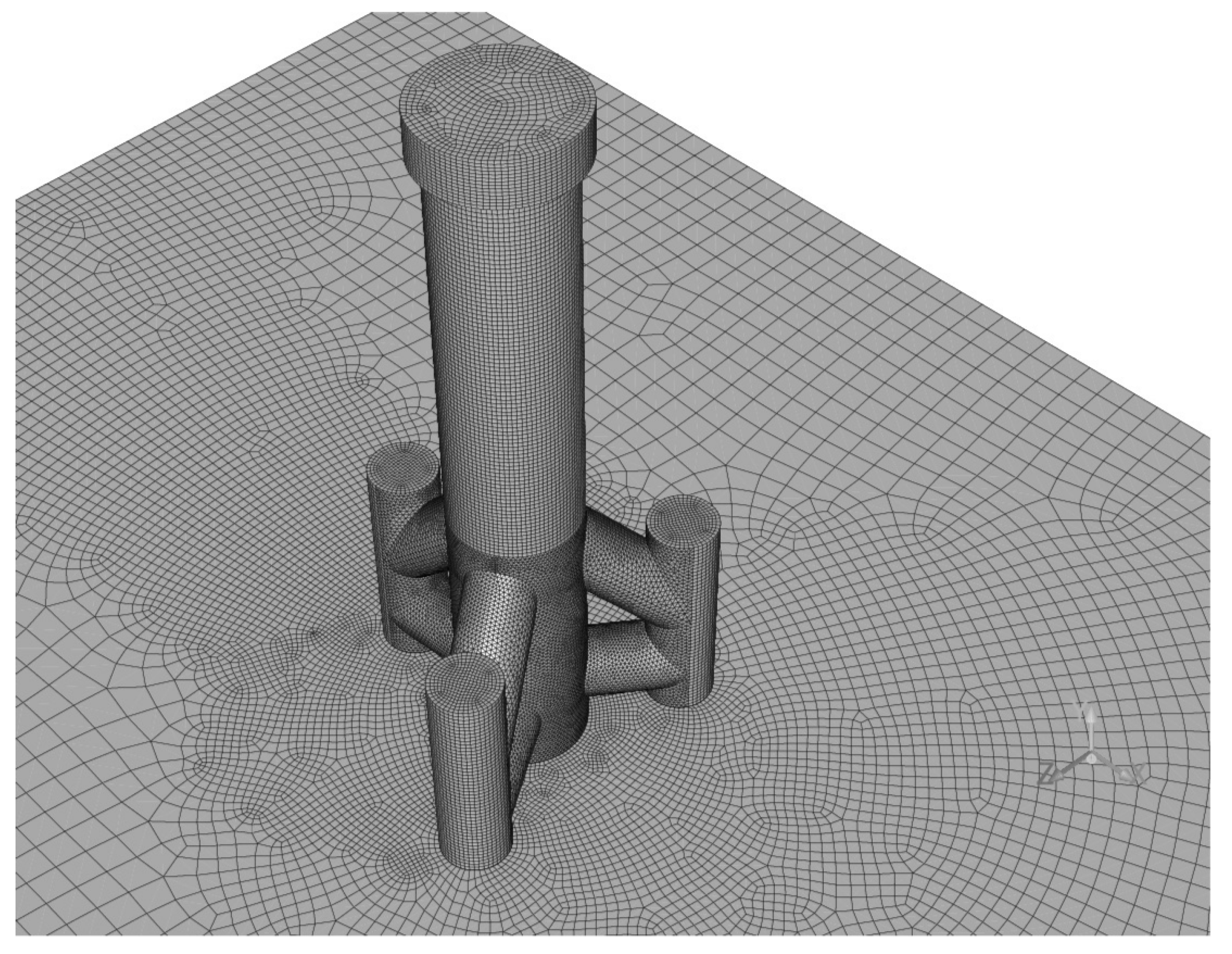
3.2. Computational Domains and Meshing

The computational domain for the simulations is centered on the foundations of the OWTs. It is structured as a rectangular box, transitioning into a sub-cylindrical volume at the outlet side, as depicted in Figure 2.

The computational domain is characterized by a length of $L=65.20$ m, an inlet width of $l=70$ m, an outlet radius of $Rout=41.3$ m and a height of $h=37$ m. The geometric configuration is specifically designed to mitigate spurious parasitic reflections by incorporating smoother transitions and favoring open angles over sharp corners at the intersections between the symmetry planes and the semi-circular outlet boundary.

Given that the primary objective of this study is to evaluate the exchange dynamics between sea wind and the structural foundations, and not to resolve finer-scale physical phenomena such as dispersive air–water interactions, passive scalar mixing, or turbulence modeling, the adopted strategy adopted to set up $y^{+}$; the dimensionless wall distance is described; the $y^{+}$ estimations is based on targeting a $y^{+}=100$ that is in the log-layer. According to ANSYS user guide, a $30\le y^{+}\le 300$ with the use of near-wall functions permits to acceptably predict flow-structure conduct; shear-stress, drag and all other fields. To that end, an adopted speed of $u=3.01$ m/s a reference that leads to wall adjacent cell centroid heights of $Y_p=0.011$ m and a Reynolds number of ${\mathcal{R}}_e=6.7·{10}^5$ for air and to $Y_p$ = $0.00092$ m and a Reynolds number of ${\mathcal{R}}_e=8.2·{10}^6$ for water. Then patched the open channel as follow; it is assumed that water dynamics will dominate below the mono-pile and tripod foundation necks downward to channel’s bed, while the wind dynamics will prevail from the mono-pile and tripod foundation necks to upward, and meshed the domain according to Yp. As illustrated in Figure 3, a structured two-dimensional mesh was applied with an exponential grading across five layers, each with a thickness of $0.5\mathrm{m}$, extending outward from the mono-pile wall. This mesh is extruded vertically along the height of the mono-pile, from the seabed up to the outlet boundary located at 37m. Adjacent to the mono-pile, three quadrilateral-paved 2D mesh layers were generated over the seabed surface and then extruded in the vertical direction along three interior planes. To further improve mesh quality and resolution, vertical refinements were introduced near the initial sea level and in proximity to the upper sections of the foundation.

For the tripod foundation, the meshing strategy involves a domain decomposition technique applied to both horizontal and vertical interior planes, as well as cylindrical segments, as depicted in Figure 2. This approach partitions the domain into sub-volumes, each optimized for the application of structured, quadrilateral-paved, or triangular mesh topologies. The delineation of these sub-regions is informed by the geometric characteristics of the structure, as represented on the surface of the tripod foundation in Figure 4.

The procedure for cells refinement between adjacent zones of dissimilar meshes obeys to halving sizes of cells; in order to comply with the philosophy behind the mesh refinement technique. The

Table 1. Summary of the mesh sizes utilized for study.

Foundations	Hexa-Hedral Cells	Quadrilateral Interior Faces
Mono-pile	1.36 M	4.005 M
Tripod	2.45 M	7.850 M

depicts the amounts of cells and their nature for each design.

3.3. Initial and Boundary Conditions

It has been long established, as initially demonstrated by [38], that the dynamics at the wind–sea interface are governed by interactions involving wave generation and variations in sea surface roughness. Subsequent research in oceanography and meteorology has consistently shown that wind velocity profiles over the ocean surface generally conform to a logarithmic distribution, as discussed by [39]. For illustrative purposes, Figure 5 presents two representative low inflow velocity profiles employed in the present study.

The occurrence of a velocity ’plateau’ reflects the assumption of a quasi-constant wind speed within the so-called neutral layer, formally referred to as the Marine Atmospheric Surface Layer MASL. The approximate bounds of this layer are indicated by the vertical green and blue lines in the figure. The velocity profiles exhibit a piecewise continuous structure, adhering to logarithmic laws in the vicinity of the MASL, while transitioning to a power-law distribution within the lower, shear-dominated oceanic boundary layer, as expressed below.

$$\left\{\begin{array}{c}u=u_0+{\displaystyle \frac{u_{\ast }}{\kappa }}·Ln\left({\displaystyle \frac{y-y_{up}}{Z_{ch}}}\right)y\ge y_{up}\hfill \\ u=u_S{y}_{lo}\le y\le y_{up}\hfill \\ u=v_0-{\displaystyle \frac{v_{\ast }}{\kappa }}·Ln\left({\displaystyle \frac{y_{lo}-y}{Z_{ch}}}\right)Z_R\le y\le y_{lo}\hfill \\ u=w_{\ast }·y·{(Z_R+y^2)}^{-1/2}0\le y\le Z_R\hfill \end{array}\right.$$

(9)

A detailed formulation and scaling of the relevant parameters are provided in [40,41]; however, only a brief overview is presented here. The quantities $u_{\ast }$ and $v_{\ast }$ stand for wind and seawater friction velocity respectively. The constant velocity $u_S$ corresponds to the characteristic wind speed within the MASL, defined over the vertical interval $[y_{lo},y_{up}]$, which is symmetrically centered around the initial mean sea level. The von Kármán constant is taken as $\kappa =0.41$, and the sea surface roughness length $Z_{ch}$ is the sea surface roughness length is prescribed using the Charnock relation [42], modified form of this relation can be found in [43] to take into account enhanced wind-stress level, while in [44] the modification considers the inclusion of the convective velocity. To ensure continuity of the velocity profile into the lower stratified ocean layers, auxiliary scaling parameters $w^{\ast }$ and $Z_R$ = 25 m are introduced as arbitrary reference velocity and depth, respectively.

3.4. Inlet Waves Boundary

A superposition of two independent inlet waves were generated via UDF routines, which are described as follow. For the first boundary wave, an oscillating wave maker consisting of a diaphragm separating seawater inlet from that of wind, initially positioned at $x_{in}=-40\mathrm{m},h_{in}=32.5\mathrm{m}$. The diaphragm is animated with a vertical oscillatory motion; at a frequency ${\omega }_d=\pi /5{\mathrm{s}}^{-1}$ with an amplitude of $y_{lo}\le a_0\le y_{up}$. The longitudinal waves generated $y_0(x,t)$ with the flap have their dispersion relation; ${\omega }_0=\omega \left(k_0\right)$ linking the frequency ${\omega }_0$ to the wave number $k_0$, assuming non-rotational flows obey to the relation below.

$$\left\{\begin{array}{c}{y}_0(x_{in},t)=h_{in}-a_o·sin({\omega }_{d}t+{\varphi }_0)-h/2\le z\le h/2\hfill \\ {({\omega }_0-k_0·u_S)}^2={\displaystyle \frac{{\rho }^{-}g·k_0+\sigma ·k_0^3}{{\rho }^{+}}}\backsimeq g·k_0+{\displaystyle \frac{\sigma ·k_0^3}{{\rho }_s}}\hfill \end{array}\right.$$

(10)

where ${\rho }^{\mp }={\rho }_s\mp {\rho }_w$g, with ${\rho }_s$ and ${\rho }_w$ are seawater and wind densities. The parameters g and $\sigma$ refer to gravity and wind-sea surface tension; showing their respective roles in the dispersion of long and short waves.

The second boundary wave $y_1(x_{in},t)$, is characterized by an amplitude $a_1=2.5\mathrm{m}$, a wave vector $k_{in}=\pi /2{\mathrm{m}}^{-1}=k\left({\omega }_{in}\right))$ and a phase ${\varphi }_1=30rd$. The prescribed wave has a dispersion relation; ${\omega }_1=\omega \left(k_1\right)$ given below.

$$\left\{\begin{array}{c}{y}_1(x_{in},t)=a_1·cos({\omega }_{in}t+{\varphi }_1)-h/2\le z\le h/2\hfill \\ {({\omega }_1-k_1·u_S)}^2=g·k_1·tanh\left(k_1{h}_{in}\right)\hfill \end{array}\right.$$

(11)

The non-linear interaction of wind-sea waves with currents of constant speed; i.e., $u_S$, is well described by Doppler-shift in the phase velocity $\omega /k$. The Doppler-effect translates into dispersion relations by simply replacing intrinsic frequencies ${\omega }_1$ with relative frequencies ${\omega }_1-k_1·u_S$, as described in [45]. In contrast to sheared current profiles; $\nabla \wedge u_S\ne \overrightarrow{0}$ in areas close to the MASL, waves dynamics exhibit unfamiliar features and complex dispersion. Concerning the remaining boundaries; the outlet pressures were imposed at the outlet boundary and at the top side surface, while symmetry plan conditions were assigned to lateral sides.

4. Numerical Results

Simulations were performed at atmospheric pressure and temperature, first with both incompressible air and water, whose properties are depicted in the

Table 2. Fluids physical properties.

Fluids	Density [kg/m3]	Dyn. Viscosity [Pa·s]	Kin. Viscosity [m2/s]
Air	1.225	$1.8·{10}^{-5}$	$1.49·{10}^{-5}$
Seawater	998.2	$1.07·{10}^{-3}$	$1.04·{10}^{-6}$

below.

The air-water surface tension coefficient was set to $\sigma =0.071\mathrm{N}/\mathrm{m}$. The pressure based solver (segregated solver) was selected for transient flow after initialization and patching with a sea level $h_{in}=32.5$ m.

Table 3. Volume of fluid model and applied solvers.

VOF Solver For Transient Open Channel
Pressure-Velocity	Spatial Discret.	Pressure
Simple	Least Square Cell Based	Presto
Momentum	Turb. Kinetic rate	Turb. Dissip. rate
2nd Upwind/3rd MUSCL	2nd Upwind/3rd MUSCL	2nd Upwind/3rd MUSCL
Volume Fraction	Level set	Transient Form
Compressive	1st Implicit/2nd Upwind	1st Order Implicit

shows the main settings adopted here.

The numerical schemes are progressively applied with increasing order as simulations proceed. Similarly the global $CFL$ number is monitored and varied within $0.55\le CFL\le 3.0$, ensuring a controlled time step for stability and the capture of waves progression.

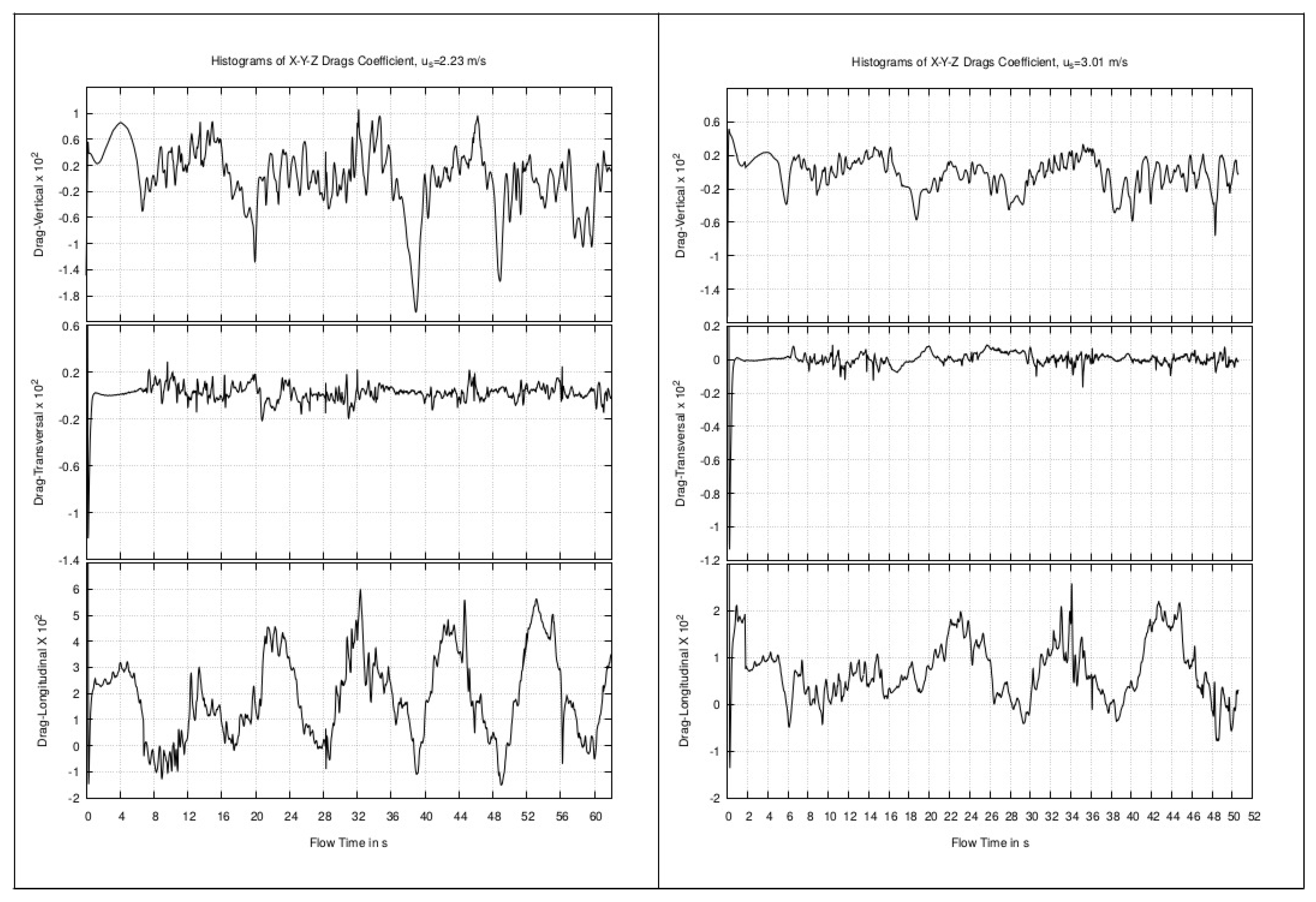
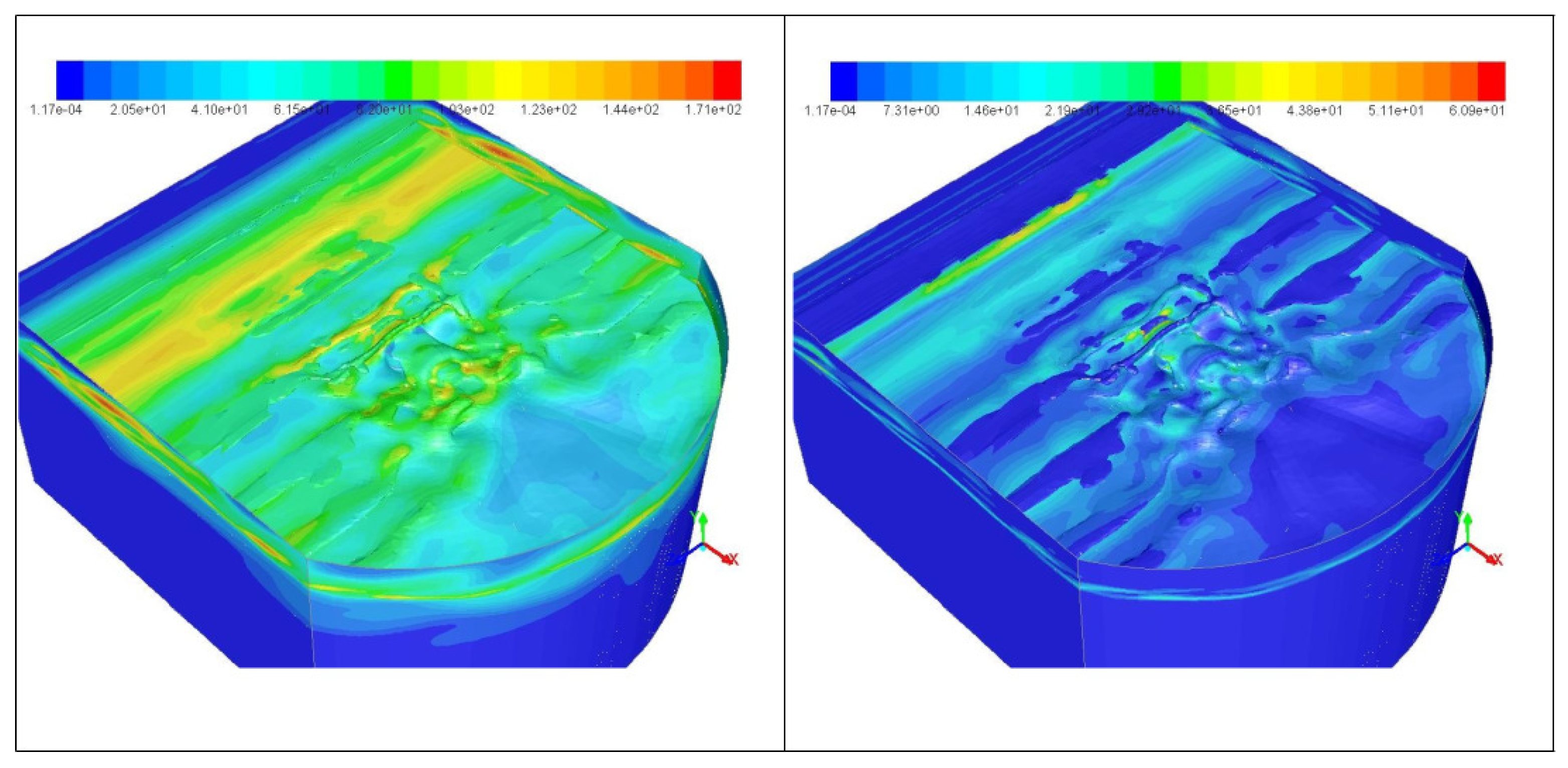
4.1. Flows Around a Mono-Pile Foundation: Cases $u_S=2.23$ and $u_S=3.01$ m/s

The qualitative results presented in Figure 6 and Figure 7 correspond to flow conditions under an initial inlet velocity of $u_S=2.23\mathrm{m}/\mathrm{s}$. In Figure 6, the overtopping behavior of incident waves interacting with the mono-pile foundation is clearly observed. The path-lines originating from the mid-plane of geometric symmetry exhibit smooth, coherent trajectories, particularly in the central region of the computational domain. A degree of deviation in streamline smoothness is observed near the lower region of the structure, particularly adjacent to the rigid channel bed. This behavior is anticipated due to the reduced water velocity in proximity to the bottom boundary.

Additional distortion of the streamlines is evident near the upper region of the mono-pile, where active wind–sea interface dynamics are at play. Momentum exchange driven by the wind occurs predominantly upstream of the foundation. As illustrated in Figure 7 (left), the velocity field beneath the interface—highlighted by red and yellow contours—reveals the presence of a localized wave-induced regime. The corresponding momentum transfer into the underlying water column is apparent in the downstream wake region, as indicated by the bluish zones extending to deeper layers in the lee of the structure.

The transitional interactions between wave motion and the monopile structure induce complex, non-equilibrium dynamic responses, leading to a redistribution of kinetic energy across the interfacial layers, as illustrated in Figure 6 (left). Figure 7 (right) further demonstrates the development of a shear stress distribution extending beyond the upper region of the foundation. The sequential snapshots presented in Figure 8, Figure 9 and Figure 10 represent the outcomes of flow dynamics simulations initiated under a prescribed inlet velocity of $u_S=3.01$ m/s. While the path-lines in Figure 8 (right) display behavior consistent with previous observations, the wind-water interface in Figure 8 (left) reveals a moderate wave slamming event at the upper section of the mono-pile. This phenomenon corresponds to a wind velocity burst captured in Figure 9 (left). Notably, the air-water interface becomes indistinct under these conditions, in contrast to the clearly defined, smooth wave regime observed in Figure 7 (left).

The transfer of wind momentum into deeper fluid layers is evident and substantiated by the distribution and magnitude of shear stress observed along the structural surface, as shown in Figure 9 (right). For initial interfacial velocities of $u_S=2.23$ m/s and $u_S=3.01$ m/s, the corresponding peak instantaneous wind velocities reach magnitudes of $20.5$ and $26.0$ m/s; as shown in Figure 7 and Figure 9 (left) respectively. Simultaneously, the velocity of the adjacent water layers in the vicinity of the foundation increases from the initial $u_S$ to approximately $5.0$ m/s and $7.0$ m/s, respectively, highlighting the role of interfacial entrainment mechanisms in facilitating momentum transfer from the wind-driven surface to the subsurface flow.

The observed reductions in velocity magnitudes above indicate a significant loss of dynamic pressure across the interface. Wall shear stress reaches peak values along the upper region of the structure, ranging between $1.8$∼$2.8·{10}^2\mathrm{kg}/(\mathrm{m}{\mathrm{s}}^2)$.

Concurrently, shear stress along the structural surface exhibits a temporally fluctuating behavior, which feeds back into the flow dynamics. While its influence on the mean flow velocity profile remains limited, the induced frictional velocity has important implications, including the generation of aero-hydrodynamic noise, excitation of structural vibrations, and accumulation of fatigue over time. Figure 10 (left) and (right) present longitudinal views of the instantaneous y-axis component of wall shear stress at successive time steps, with peak magnitudes in the range of $3.2$∼$4.6·{10}^2\mathrm{kg}/(\mathrm{m}{\mathrm{s}}^2)$. Notably, these maxima are concentrated near the neck region of the structure, an area strongly influenced by wind–water interfacial interactions.

The hydrodynamic force ${\overrightarrow{\mathcal{T}}}_s$ (traction) exerted on the foundation’s unit surface is basically computed from the expression of the shear stress in the Equation (4), that is

$$\begin{array}{ccc}{\overrightarrow{\mathcal{T}}}_s& =& \mathcal{T}·{\widehat{n}}_s\hfill \\ & =& \left(-p·I_d+\mu ·(\nabla \overrightarrow{u}+\nabla {\overrightarrow{u}}^T)+\lambda (\nabla ·\overrightarrow{u})·I_d\right)·{\widehat{n}}_s\hfill \end{array}$$

(12)

where ${\widehat{n}}_s$ is the outward unit normal to the structure, the mechanical pressure $p_m$ exerted on the unit surface is defined as the first invariant of the stress tensor and is related to the thermodynamic pressure p as follows

$$\begin{array}{ccc}{p}_m& =& -{\displaystyle \frac{1}{3}}trace\left(\mathcal{T}\right)\hfill \\ & =& p-\eta \nabla ·\overrightarrow{u}\hfill \end{array}$$

(13)

The equivalence between the two pressures does not hold in compressible regions of the flow; as in near wind-water interface, but holds in outer regions; as in the bulk of the incompressible fluids involved. The tangential part of the traction ${\overrightarrow{\mathcal{T}}}_t$ is a vector field that is tangent to the foundation everywhere, it provides details of the flow on the structure, and is given by

$$\begin{array}{ccc}{\overrightarrow{\mathcal{T}}}_t& =& {\overrightarrow{\mathcal{T}}}_s-({\overrightarrow{\mathcal{T}}}_s·{\widehat{n}}_s)·{\widehat{n}}_s\hfill \end{array}$$

(14)

The wall shear stress, denoted as ${\mathcal{T}}_w=\parallel {\overrightarrow{\mathcal{T}}}_t\parallel$, is directly related to the friction velocity, defined by $u^{\ast }=\sqrt{{\mathcal{T}}_w/\rho }$, a fundamental parameter for scaling turbulent flows.

Conventional estimates of drag coefficients are typically derived under assumptions of vertical homogeneity and idealized conditions—namely, periodicity and steady-state flow. In contrast, the present study evaluates the directional drag coefficients per unit surface area under pseudo-periodic flow conditions. The histograms of the longitudinal ${\widehat{C}}_{D\Vert }$, transverse ${\widehat{C}}_{D⊢}$ and vertical ${\widehat{C}}_{D\perp }$ drag coefficients are are computed while accounting for temporal and spatial variability of the wind–water interface, as illustrated in Figure 11. This approach aims to more accurately characterize the dynamic response of the mono-pile foundation under unsteady flow conditions, thereby revealing the onset of directional anisotropy and preferential motion alignment.

Inspection of Figure 11 indicates that the longitudinal ${\widehat{C}}_{D\Vert }$ (bottom left and right) and vertical ${\widehat{C}}_{D\perp }$ (top left and right) drag coefficient histograms display significant variability and fluctuations about mean values of approximately $1.92·{10}^2$ and $0.63·{10}^2$ respectively.

In contrast, the histograms of the transverse drag coefficient ${\widehat{C}}_{D⊢}$, shown in Figure 11 (middle left and right), exhibit minimal variation and fluctuation around the respective mean values of $8.3·{10}^{-2}$ and $3.4·{10}^{-1}$; suggesting limited re-circulatory activity in the transverse direction. Conversely, the vertical drag coefficient ${\widehat{C}}_{D\perp }$ demonstrates pronounced variability, with fluctuations centered around mean values of approximately $2.23$ and $-3.92$, indicating a more dynamic vertical response.

It is noteworthy that the temporal fluctuations in the longitudinal drag coefficient ${\widehat{C}}_{D\Vert }$ exhibit a predominantly positive bias, in contrast to the vertical drag coefficient ${\widehat{C}}_{D\perp }$, whose variations do not display a preferential direction. This latter behavior suggests the presence of vertical momentum exchange between the atmospheric boundary layer and the underlying water column. As evidenced in Figure 10 (left and right), these exchange processes appear to be particularly intense in the vicinity of the wind–water interface.

The histograms of pressure and shear rate presented in Figure 12 (left and right) clearly demonstrate that their magnitudes remain largely insensitive to the increase in the initial wind–water interface velocity. Notable exceptions to this trend are observed in the dynamic pressure—which, as expected, responds directly to variations in flow intensity—and the skin friction factor. The latter exhibits a significant reduction in magnitude, with values approximately an order of magnitude lower, and a decrease in the mean from $1.65·{10}^{-2}$ to $6.68·{10}^{-3}$, indicating a notable decline in near-wall shear stress and frictional effects under increased flow conditions.

In the following figures (Figure 13 and Figure 14), the distribution of the empirical turbulence intensity exhibit peaks of $1.7·{10}^2$ just above the water skin; i.e., mainly in the air layer away from the the mono-pile and tripod foundation. Near the the mono-pile and tripod foundations, localized lower turbulence intensity is taking place. The general trend of variations in both turbulence intensity and vorticity magnitude show a low level of activity except in the near-field of the mono-pile.

The distribution of turbulent kinetic energy and especially the rate of the turbulence dissipation reaches peaks of dissipation rate at the vicinity of the mono-pile which acting as obstacle.

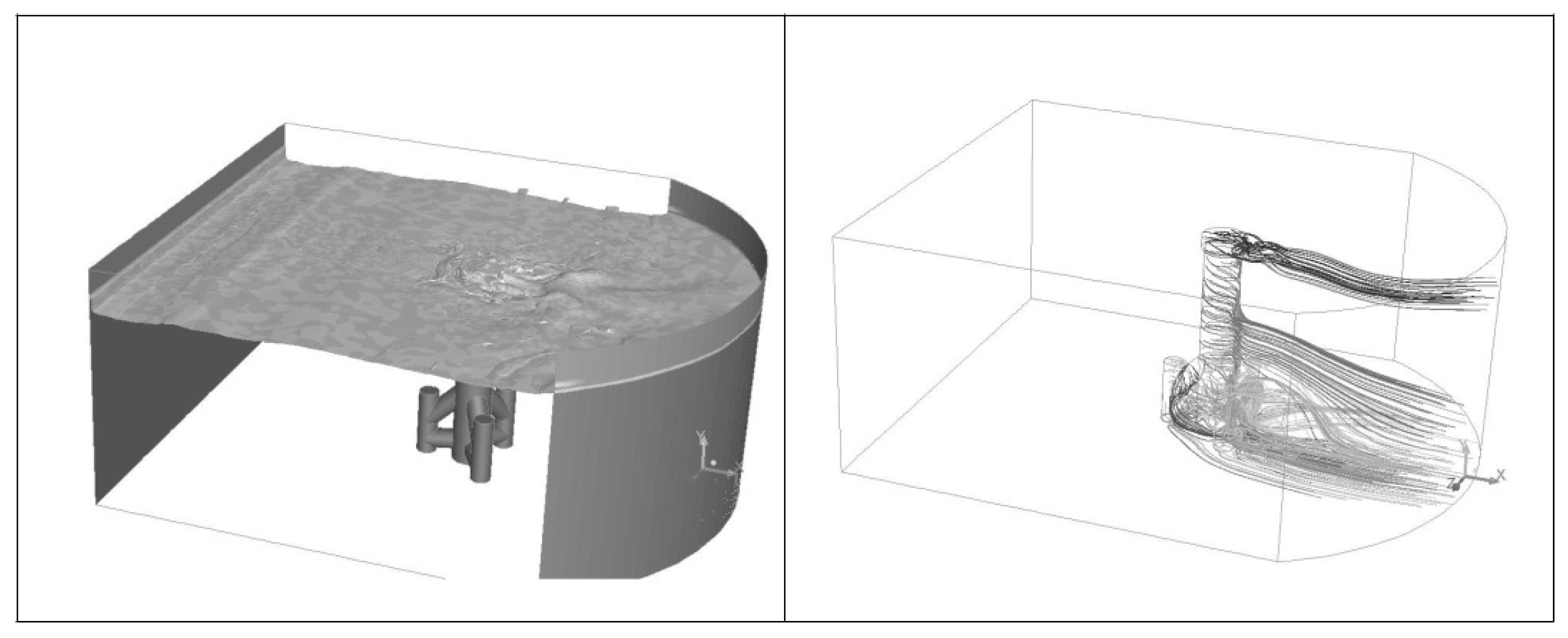
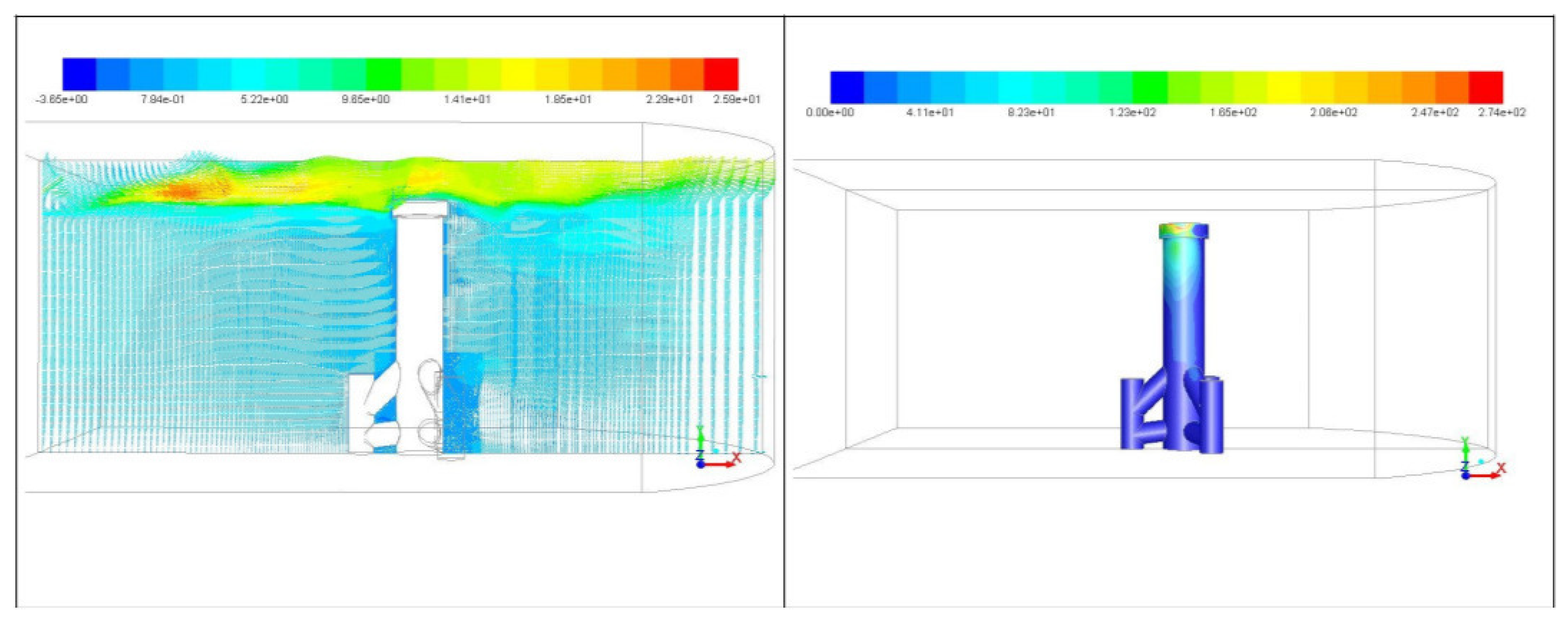
4.2. Flow Around a Tripod Foundation: Case $u_S=3.01$ m/s

The qualitative results presented in Figure 15 (left and right) pertain to the tripod foundation subjected to a wind–water flow with an initial velocity of $u_S=3.01$ m/s. The left diagram illustrates a disturbed, wavy wind–water interface in proximity to the tripod foundation.

The streamlines exhibit three-dimensional characteristics, resulting in a complex flow structure in the region near the seabed, influenced by the intricate design of the supporting structures. The flow appears to accelerate downward before transitioning to a predominantly horizontal, two-dimensional configuration over a relatively short distance.

As depicted in Figure 16 (left), the wind velocity reaches approximately ≈26.0 m/s upstream of the structure. The velocity field illustrates a transitional flow regime, shifting from a wavy state upstream to a nearly stratified flow regime downstream of the structure. There is a noticeable reduction in velocity to around ∼5.0 m/s in the immediate vicinity of the tripod, while the upper water layers near the foundation experience a gain in momentum, with velocity increasing to approximately ≈6.0 m/s, which is double the initial magnitude.

The wall shear stress distribution shown in Figure 16 (right) exhibits a trend comparable to that observed for the mono-pile foundation, with an instantaneous peak value of $2.7·{10}^2\mathrm{kg}/(\mathrm{m}{\mathrm{s}}^2)$ closely matching the corresponding maximum value computed for the mono-pile case, $2.8·{10}^2\mathrm{kg}/(\mathrm{m}{\mathrm{s}}^2)$. The vertical components of wall shear stress, depicted in Figure 17 (left and right), reach peak magnitudes of $37.5\mathrm{kg}/(\mathrm{m}{\mathrm{s}}^2)$ and $2.06·{10}^2\mathrm{kg}/(\mathrm{m}{\mathrm{s}}^2)$ at successive time instants.

It is important to highlight that achieving numerical stability for the flow simulation in this case posed significant challenges, primarily due to the complex geometry of the domain, which directly influences the underlying mesh quality, and the contrasting physical properties of the interacting fluids—particularly the large disparity in viscosity and density across the wind–water interface. Additionally, the pseudo-periodic nature of the wave-induced initial conditions likely contributed to the numerical instability. Despite these complexities, a stable simulation was successfully attained over a full flushing time of $36.0$ s. This was achieved through careful control of the time-stepping scheme, specifically by tuning the global $CFL$ number and adjusting the number of iterations per time step. The histograms presented in Figure 18, corresponding to key flow variables around the tripod foundation, indicate that the skin friction factor attains values nearly an order of magnitude higher than those previously reported in Figure 12 (right). In contrast, the dynamic pressure and strain rate distributions remain within comparable ranges, suggesting localized intensification of wall-bounded shear without a substantial change in bulk flow dynamics.

The recorded variations of the directional drag coefficients per unit surface; ${\widehat{C}}_{D\Vert }$, ${\widehat{C}}_{D⊢}$ and ${\widehat{C}}_{D\perp }$ are presented in Figure 18 (right). The temporal variations of ${\widehat{C}}_{D\Vert }$ reveals predominantly positive fluctuations centered around a mean value of $1.72·{10}^2$, indicating a sustained net momentum transfer in the streamwise direction. The behavior of ${\widehat{C}}_{D⊢}$ exhibits indications of low-frequency oscillations in the transverse z-axis direction, suggesting the presence of weak lateral flow instabilities. In contrast, the histogram of ${\widehat{C}}_{D\perp }$ displays a clear bias toward negative values, fluctuating around a mean of $-6.62·{10}^{-2}$, which is indicative of a dominant downward re-circulatory motion in the vicinity of the tripod foundation. This observed trend raises an important question regarding the relationship between the negative vertical drag contributions and the transitional streamline behavior documented in Figure 15, particularly near the seabed region surrounding the tripod structure.

Below (Figure 19 and Figure 20), the distributions of the empirical turbulence intensity exhibit peaks comparable to those observed fo the mono-pile just above the water skin. These are also localized in the air layer away from the tripod. A localized lower level of turbulence intensity is taking place near the tripod. The distribution of the vorticity magnitude exhibits activity mainly at the inlet and above the water skin.

The main activity in the distributions of the turbulent kinetic energy is shown to be taking place just above the interface, with apeak of $3.0·{10}^1$, in contrary to the behavior of the rate of dissipation; a concentrated dissipation; which is localized at the top of the tripod.

5. Analyses via Reynolds ${\mathcal{R}}_e$ and Froude Numbers ${\mathcal{F}}_r$

It is of relevance to look at the abrupt changes in velocities of the wind-water layers depicted in Figure 7, Figure 9 and Figure 16, in terms of Reynolds number; ${\mathcal{R}}_e$, and of Froude number; ${\mathcal{F}}_r$. In the context of this study, which focuses on the momentum and energy exchange within the wind-sea-foundations, the analysis emphasizes global phasic parameters rather than localized (wall shear or frictional) flow descriptors such as Reynolds and Froude numbers.

Table 4. Maximum phasic Reynolds numbers.

			Maximum Reynolds Phasic Numbers
	Mono-Pile		Mono-Pile		Tripod
	${\mathit{u}}_{\mathit{S}}=\mathbf{2.23}$ m/s		${\mathit{u}}_{\mathit{S}}=\mathbf{3.01}$ m/s		${\mathit{u}}_{\mathit{S}}=\mathbf{3.01}$ m/s
$max\left(u_w\right)$	20.5		26.0		26.0
max $({\mathcal{R}}_{ew})$	$5.4·{10}^7$		$7.6·{10}^7$		$\hspace{1em}\hspace{1em}7.6·{10}^7$
$max\left(u_s\right)$	5.0		7.0		6.0
max $({\mathcal{R}}_{es})$	$2.08·{10}^8$		$2.9·{10}^8$		$\hspace{1em}\hspace{1em}2.5·{10}^8$

presents the Reynolds numbers for the wind Reynolds numbers $R_{ew}$ and $R_{es}$ phases, which serve as indicators of their respective flow regimes. These values are computed based on the maximum phasic velocities and a representative hydraulic radius for the water phase, defined as $D_H=2·{\displaystyle \frac{lh}{l+h}}\simeq 43.9$ m; where l and h denote the characteristic horizontal and vertical dimensions of the flow domain.

The observation from above shows that, ratios of 3∼4 times are reached between maximum phasic Reynolds numbers, turbulence is forced throughout the water volume driven by the wind entrainment with the presence of static obstacles. The increase in phasic Reynolds numbers at both sides of the interface is synonymous of kinetic energy transfer from wind and waves to upper water layers.

With regard to the Froude, it is important to note that various formulations exist in the literature under this designation; however, several of these expressions exhibit significant limitations. In particular, defining a dynamically meaningful Froude number for interfacial flows in open channel systems proves challenging without explicitly accounting for the influence of static structures. The complexity arises from the inherently coupled nature of wind-driven surface dynamics and underlying hydrodynamic interactions, which are strongly modulated by structural constraints at or near the interface. The sub-critical nature of the actual flows can be seen from the initial value of Froude number; i.e., $0.12\le {\mathcal{F}}_r={\displaystyle \frac{u_S}{\sqrt{g·h_{in}}}}\le 0.17$.

The importance of Froude number resides in its close link to water entrainment ratio as shown by [46], and parametrized by [47] with the use of a large dataset collected from field measurements and laboratory experiments. Furthermore, in an earlier work in [48]; the authors reported a strong monotonic dependence between the entrainment ratio and Reynolds number. The entrainment coefficient relates the ratio of the wind vertical velocity component $w_w$ over the magnitude of wind velocity; i.e., $E_r=w_w/u_w$. It is a key flow parameter for the integrity of pre-stressed structures under large bulk loads of important water masses in motion under entrainment.

According to [49,50,51] and others, the available energy flux into the sea surface is due to the relative wind stress; ${\mathcal{T}}_{ws}^R$ parametrized through an inter-facial drag coefficient $C_{Int}$ and a drift velocity; i.e., $\Delta {\overrightarrow{u}}_D={\overrightarrow{u}}_w-{\overrightarrow{u}}_s$; between the wind speed $u_w$ and the sea surface velocity; $u_s\ncong u_S$ as follow

$$\begin{array}{ccc}{\overrightarrow{\mathcal{T}}}_{ws}^R& =& {\rho }_w·C_{Int}·\Delta {\overrightarrow{u}}_D·|\Delta {\overrightarrow{u}}_D|\hfill \end{array}$$

(15)

The resulting wind power input per unit volume is given by, [52],

$$\begin{array}{ccc}{P}_k& =& {\overrightarrow{\mathcal{T}}}_{ws}^R·{\overrightarrow{u}}_s\hfill \\ & =& {\rho }_w·C_{Int}·\Delta {\overrightarrow{u}}_D·|\Delta {\overrightarrow{u}}_D|·{\overrightarrow{u}}_s\hfill \end{array}$$

(16)

6. Conclusions

• This study aimed to evaluate the exchange dynamics between wind-driven surface flows and offshore foundation structures, with a focus on the interaction at structural interfaces rather than on small-scale turbulent processes such as those characterized by $y^{+}$ passive mixing, or detailed turbulence intensity distributions. The flow conditions employed in the simulations do not replicate extreme wind-sea scenarios but serve instead to investigate fundamental hydrodynamic responses under idealized, pseudo-periodic wave inlets. This approach introduces variability in the inflow conditions, enabling the observation of anisotropic flow-structure interactions under steady unidirectional flow.
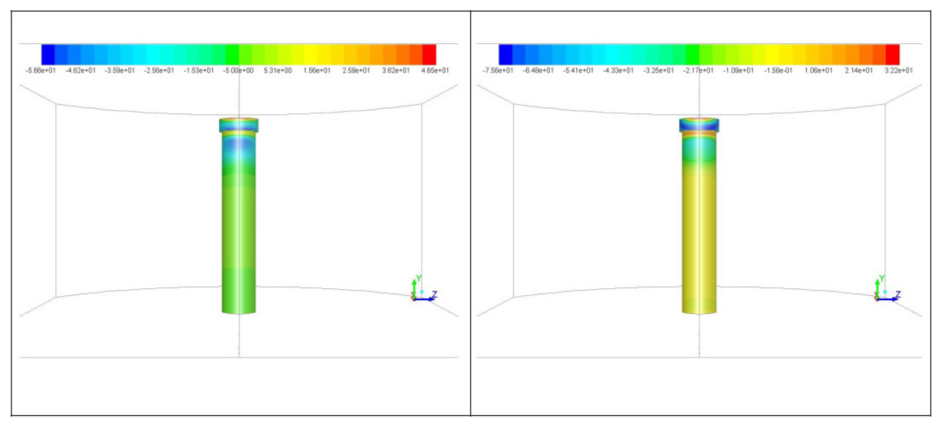
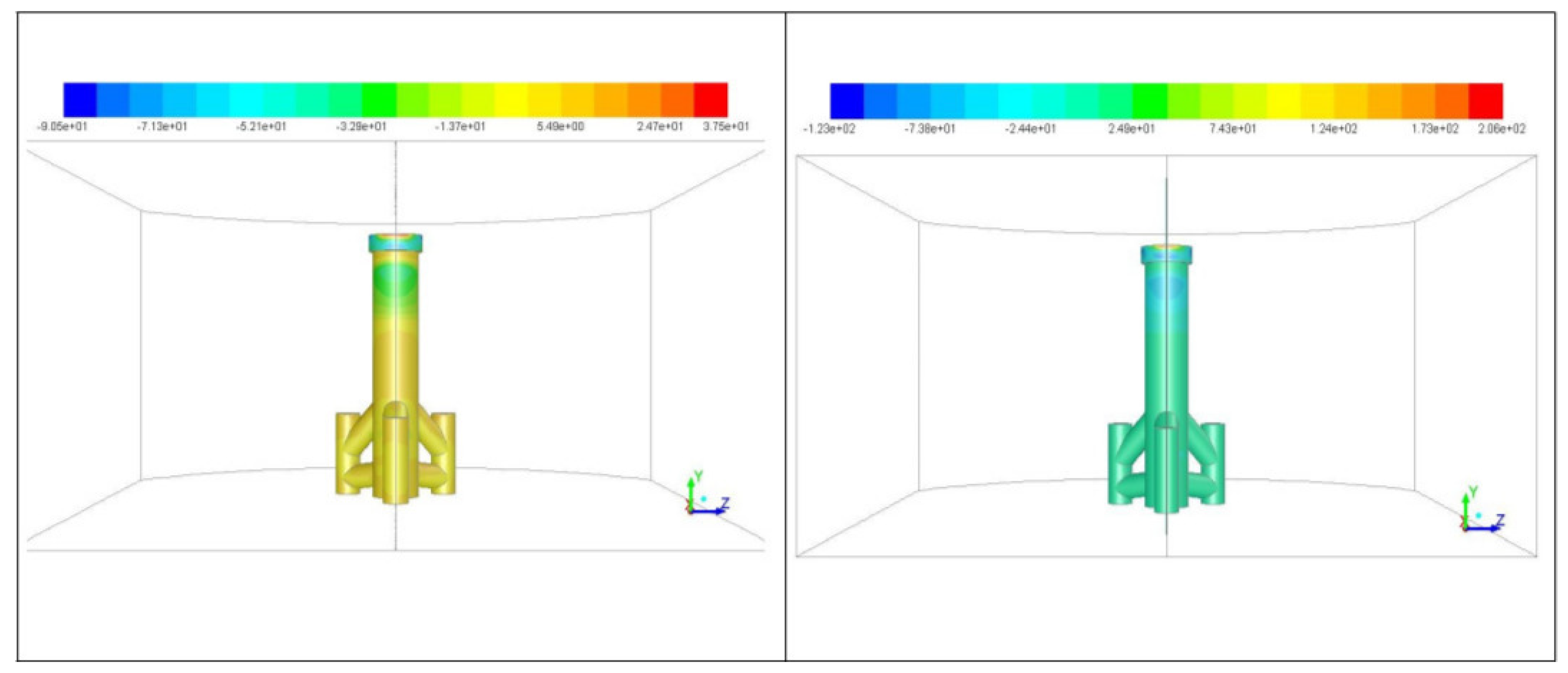
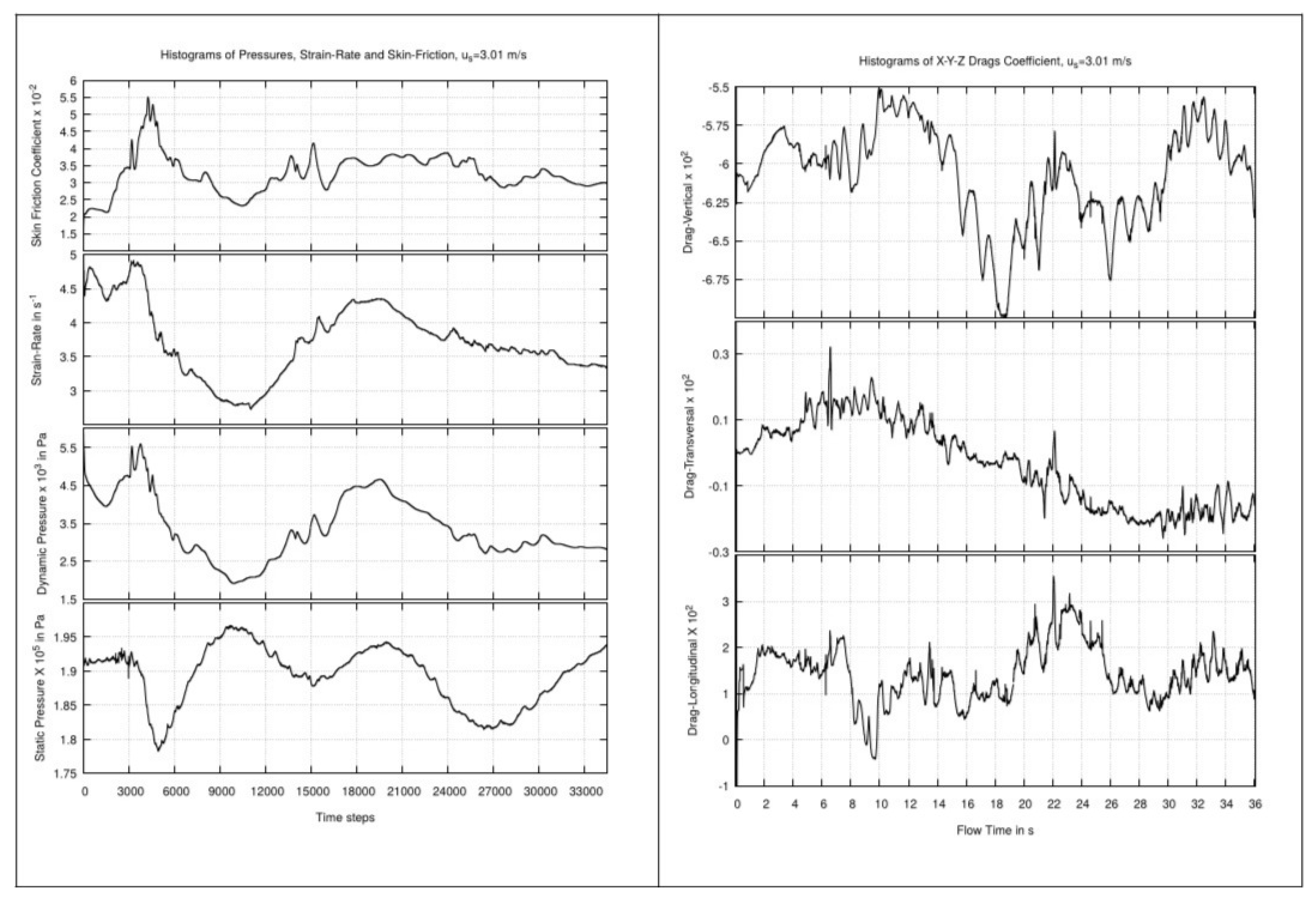
• The simulation results demonstrate that vertical wall-shear stress distributions exhibit periodic peaks along the structural surfaces, with concentration zones at the neck and upper portions of the foundations—regions where flow-interface interactions are most intense. Analysis of directional drag coefficients reveals high-frequency variations, with each directional component showing a distinct pattern. This indicates that the foundations are subject to anisotropic force distributions, which have implications for structural stability and fatigue over time.
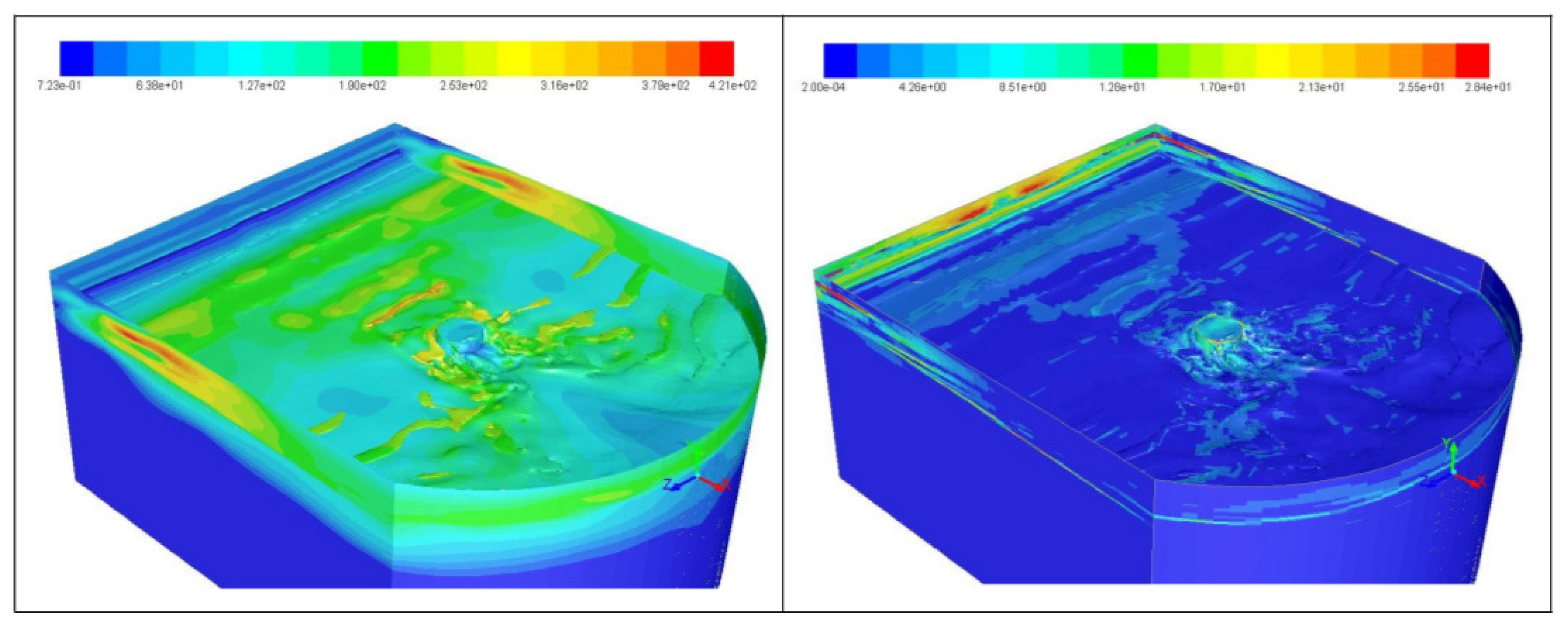
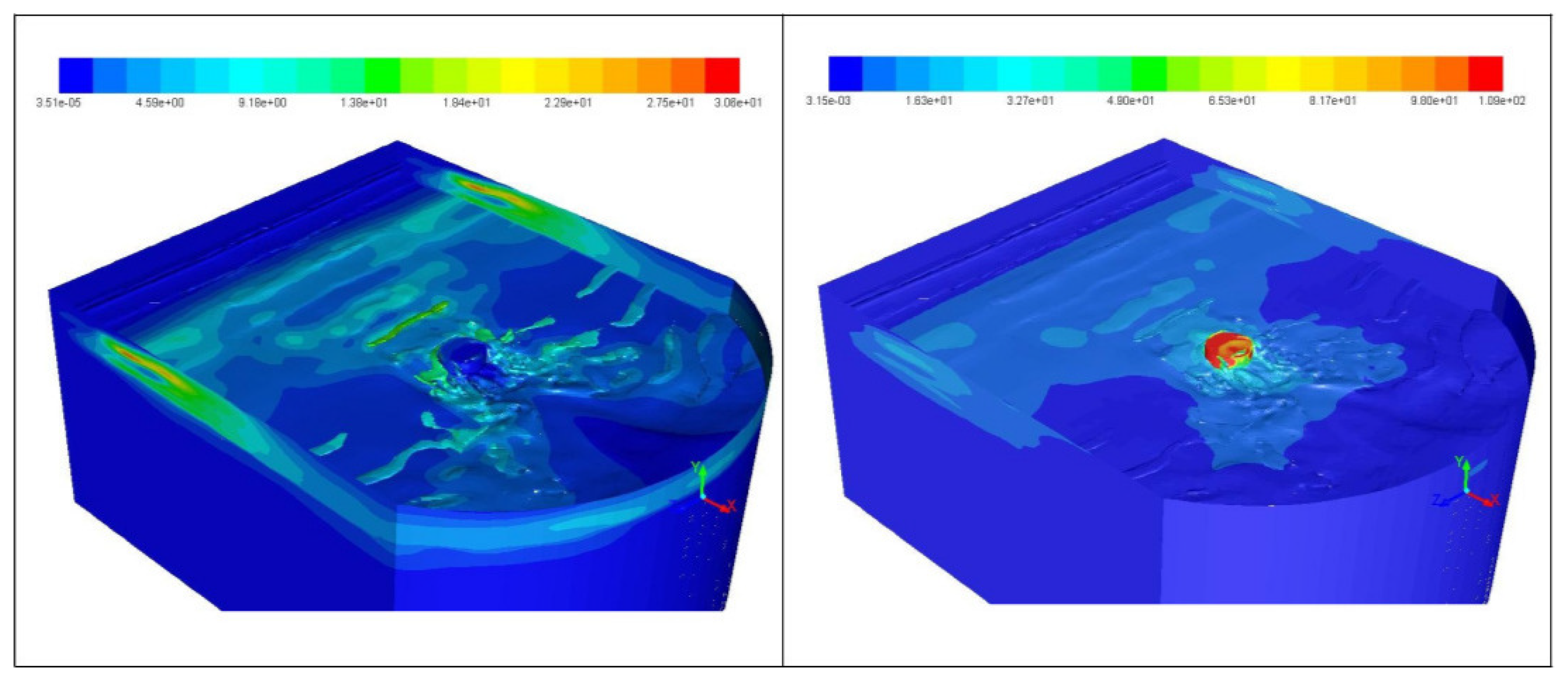
• The behavior of the vertical drag coefficient further reveals the presence of vertical flow structures that facilitate exchange between upper and lower water layers. These vertical dynamics not only influence foundation loading but also affect local hydrodynamics and potentially disrupt the stratification of water density. While the magnitude of these effects warrants careful quantification, their broader implications must be considered in the context of large OWT farms, particularly regarding long-term environmental impacts such as salinity changes and effects on marine ecosystems.
• Additionally, localized phenomena such as down-welling—particularly observed in tripod configurations—suggest that vertical downward flow and flow convergence near the seabed require further investigation to confirm and characterize these dynamics.
• It is important to minimize negative effects of OWT on marine ecosystems while maximizing constructive ones. The uncertainty of long-term effects of OWT remain difficult to grasp or to quantify. All the required studies for understanding the effects of OWT farms on climate and on marine life, must involve sea users, companies, scientists and legislators to establish appropriate and stricter rules for the good of the environment.

References

1. Seebai, T.S.; Sundaravadivelu, R. Response analysis of spar platform with wind turbine. Ships Offshore Struct. 2013, 8, 94–101. [Google Scholar]
2. Wunsch, C.; Ferrari, R. Is the ocean speeding up? Ocean surface energy trends. J. Phys. Oceanogr. 2020, 50, 3205–3217. [Google Scholar] [CrossRef]
3. Kurian, V.J.; Ng, C.Y.; Liew, M.S. Dynamic responses of truss spar due to wave actions. Res. J. Appl. Sci. Eng. Technol. 2013, 5, 812–818. [Google Scholar] [CrossRef]
4. Shi, Q.; Borassa, M. Coupling Ocean Currents and Waves with Wind Stress over the Gulf Stream. Remote Sens. 2019, 11, 1476. [Google Scholar] [CrossRef]
5. Wang, X.; Zeng, X.; Li, J.; Yang, X.; Wang, H. A review on recent advancements of substructures for offshore wind. Energy Convers. Manag. 2018, 158, 103–119. [Google Scholar] [CrossRef]
6. Haider, R.; Shi, W.; Cai, Y.; Lin, Z.; Li, X.; Hu, Z. A comprehensive numerical model for aero-hydro-mooring analysis of a floating offshore wind turbine. Renew. Energy 2024, 237, 121793. [Google Scholar] [CrossRef]
7. Haider, R.; Shi, W.; Lin, Z.; Cai, Y.; Zhao, H.; Li, X. Coupled analysis of floating offshore wind turbines with new mooring systems by CFD method. Ocean. Eng. 2024, 312 Pt 1, 119054. [Google Scholar] [CrossRef]
8. Christensen, E.D.; Bredmose, H.; Hansen, E.A. Extreme wave forces and wave run-ups on offshore wind turbine foundations. In Proceedings of the Copenhagen Offshore Wind 2005, Copenhagen, Denmark, 26–28 October 2005; pp. 1–10. [Google Scholar]
9. Bredmose, H.; Jacobsen, N.G.; Hansen, E.A. Breaking wave impacts on offshore wind turbine foundations:Wave groups and CFD. In Proceedings of the International Conference on Offshore Mechanics and Arctic Engineering, Shanghai, China, 6–11 June 2010; pp. 397–404. [Google Scholar]
10. Chen, D.; Huang, K.; Bretel, V.; Hou, L. Comparison of structural properties between mono-pile and tripod offshore wind-turbine support structures. Adv. Mech. Eng. 2013, 2013, 175684. [Google Scholar] [CrossRef]
11. Alesbe, I.; Maksoud, M.A.; Aljabair, S. Comparison of structural properties between mono-pile and tripod offshore wind-turbine support structures. J. Renew. Energy 2016, 2, 1–12. [Google Scholar]
12. Lai, R.J.; Shemdin, O. Laboratory investigation of air turbulence above simple water wave. J. Geophys. Res. 1971, 76, 7334–7350. [Google Scholar] [CrossRef]
13. Veron, F.; Saxena, G.; Misra, S.K. Measurements of the viscous tangential stress in the airflow above wind waves. Geophys. Res. Lett. 2007, 34, 281–314. [Google Scholar] [CrossRef]
14. Buckley, M.P.; Veron, F. Structure of the airflow above surface waves. J. Phys. Oceanogr. 2016, 46, 1377–1397. [Google Scholar] [CrossRef]
15. Buckley, M.P.; Veron, F. The turbulent airflow over wind generated surface waves. Eur. J. Mech. (B/Fluids) 2019, 73, 132–143. [Google Scholar] [CrossRef]
16. Shemer, L. On Evolution of Young Wind Waves in Time and Space. Atmosphere 2019, 10, 562. [Google Scholar] [CrossRef]
17. Flugge, M.; Bakhoday-Paskyabi, M.; Reuder, J.; El Guernaoui, O. Wind Stress in the Coastal Zone: Observations from a Buoy in Southwestern Norway. Atmosphere 2019, 10, 491. [Google Scholar] [CrossRef]
18. Laxague, N.; Zappa, C. Observations of mean and wave orbital flows in the ocean’s upper centimetres. J. Fluid Mech. 2020, 887, A10. [Google Scholar] [CrossRef]
19. Grachev, A.; Fairall, C. Upward momentum transfer in the marine boundary layer. J. Phys. Oceanogr. 2001, 31, 1698–1711. [Google Scholar] [CrossRef]
20. Kahma, K.K.; Donelan, M.A.; Drennan, W.M.; Terray, E.A. Evidence of energy and momentum flux from swell to wind. J. Phys. Oceanogr. 2016, 46, 2143–2156. [Google Scholar] [CrossRef]
21. Sullivan, P.P.; Mcwilliams, J.C.; Moeng, C.-H. Simulation of turbulent flow over idealized water waves. J. Fluid Mech. 2000, 404, 47–85. [Google Scholar] [CrossRef]
22. Yang, D.; Shen, L. Direct numerical simulation of scalar transport in turbulent flows over progressive surface waves. J. Fluid Mech. 2017, 819, 58–103. [Google Scholar] [CrossRef]
23. Yang, Z.; Deng, B.Q.; Shen, L. Direct numerical simulation of wind turbulence over breaking waves. J. Fluid Mech. 2018, 850, 120–155. [Google Scholar] [CrossRef]
24. Sullivan, P.; Banner, M.L.; Morisson, R.P.; Peirson, W.L. Turbulent Flow over Steep Steady and Unsteady Waves under Strong Wind Forcing. J. Phys. Oceanogr. 2018, 48, 3–27. [Google Scholar] [CrossRef]
25. Akervik, E.; Vartdal, M. The role of wave kinematics in turbulent flow over waves. J. Fluid Mech. 2021, 919, 890–915. [Google Scholar] [CrossRef]
26. Cao, T.; Shen, L. A numerical and theoretical study of wind over fast-propagating water waves. J. Fluid Mech. 2021, 919, A38. [Google Scholar] [CrossRef]
27. Hao, X.; Hen, L. Wind–wave coupling study using LES of wind and phase-resolved simulation of nonlinear waves. J. Fluid Mech. 2019, 874, 391–425. [Google Scholar] [CrossRef]
28. Wang, L.; Zhang, W.; Hao, X.; Huang, W.; Shen, L.; Xu, C.; Zhang, Z. Surface wave effects on energy transfer in overlying turbulent flow. J. Fluid Mech. 2020, 951, A21. [Google Scholar] [CrossRef]
29. Wu, J.; Popinet, S.; Deike, L. Revisiting wind wave growth with fully-coupled direct numerical simulations. J. Fluid Mech. 2022, 951, A18. [Google Scholar] [CrossRef]
30. Cimarelli, A.; Romoli, F.; Stalio, E. On wind–wave interaction phenomena at low Reynolds numbers. J. Fluid Mech. 2023, 956, A13. [Google Scholar] [CrossRef]
31. Guth, S.; Katsidoniotaki, E.; Themistoklis, P.; Sapsis, P.T. Statistical modeling of fully nonlinear hydrodynamic loads on offshore wind turbine mono-pile foundations using wave episodes and targeted CFD simulations through active sampling. Wind Energy. 2020, 27, 75–100. [Google Scholar] [CrossRef]
32. Eames, I.; Robinson, T. Free-surface channel flow around a square cylinder. J. Fluid Mech. 2024, 980, A16. [Google Scholar] [CrossRef]
33. Chen, H.; Zou, Q. Effects of following and opposing vertical current shear on nonlinear wave interactions. Appl. Ocean Res. 2019, 89, 23–35. [Google Scholar] [CrossRef]
34. Lange, M.; Focken, U. Physical Approach to Short-Term Wind Power Prediction; Springer: Berlin/Heidelberg, Germany, 2005; ISBN 3-540-25662-8. [Google Scholar] [CrossRef]
35. Emeis, S. Wind Energy Meteorology, 2nd ed.; Springer: Cham, Switzerland, 2018; ISBN 978-3-319-72858-2. [Google Scholar] [CrossRef]
36. Fluent. In ANSYS Fluent 16.5 User’s Guide; ANSYS, Inc.: Canonsburg, PA, USA, 2015.
37. Menter, F.R. Two-Equation Eddy-Viscosity Turbulence Models for Engineering Applications. AIAA J. 1994, 32, 1598–1605. [Google Scholar] [CrossRef]
38. Stewart, R.W. The wave drag of wind over water. J. Fluid Mech. 1961, 10, 189–194. [Google Scholar] [CrossRef]
39. Bye, J.A.T. The Dynamics of Air-Sea Boundary Layer. Adv. Environ. Eng. Res. 2023, 4, 1–16. [Google Scholar] [CrossRef]
40. Businger, J.A. The Marine Boundary Layer, from Air-Sea Interface to Inversion; Technical Report NCAR/TN-252 + STR NCAR; National Center for Atmospheric Research: Boulder, CO, USA, 1985. [Google Scholar]
41. Bye, J.A.T. The coupling of wave drift and wind velocity profiles. J. Mar. Res. 1988, 46, 457–472. [Google Scholar] [CrossRef]
42. Bye, J.A.T.; Wolff, J.O. Charnock dynamics: A model for the velocity structure in the wave boundary layer of the air–sea interface. Ocean Dyn. 2008, 58, 31–42. [Google Scholar] [CrossRef]
43. Janssen, P. Quasilinear theory of wind-wave generation applied to wave forecasting. J. Phys. Oceanogr. 1991, 21, 1631–1642. [Google Scholar] [CrossRef]
44. Abdella, K.; D’Alessio, S. A parameterization of the roughness length for the air-sea interface in free convection. Environ. Fluid Mech. 2003, 3, 55–77. [Google Scholar] [CrossRef]
45. Peregrine, D.H.; Jonsson, G.I. Interaction of Waves and Currents; Technical Report NO. 83-6; Coastal Engineering Research Center: Fort Belvoir, VA, USA, 1983. [Google Scholar]
46. Wells, M.; Cenedese, C.; Caulfield, C.P. The Relationship between Flux Coefficient and Entrainment Ratio in Density Currents. Am. Meteo. Soc. 2010, 40, 2713–2727. [Google Scholar] [CrossRef]
47. Cenedese, C.; Adduce, C. A new parametrization for entrainment in overflows. J. Phys. Oceanogr. 2010, 40, 1835–1850. [Google Scholar] [CrossRef]
48. Cenedese, C.; Adduce, C. Mixing in a density-driven current flowing down a slope in a rotating fluid. J. Fluid Mech. 2008, 604, 369–388. [Google Scholar] [CrossRef]
49. Faller, A.J. Sources of energy for the ocean circulation and a theory of the mixed layer. In Proceedings of the Fifth United States Congress of Applied Mechanics, American Society of Mechanical Engineers, Minneapolis, MN, USA, 14–17 June 1966; pp. 651–672. [Google Scholar]
50. Oort, A.H.; Anderson, L.A.; Peixoto, J.P. Estimates of the energy cycle of the oceans. J. Geophys. Res. 1994, 99, 7665–7688. [Google Scholar] [CrossRef]
51. Wunsch, C.; Ferrari, R. Vertical mixing, energy, and the general circulation of the oceans. Annu. Rev. Fluid Mech. 2004, 36, 281–314. [Google Scholar] [CrossRef]
52. Large, W.G.; Yeager, S.G. Diurnal to Decadal Global Forcing for Ocean and Sea-Ice Models: The Data Sets and Flux Climatologies; Technical Report 434, NCAR Tech Note NCAR/TN-460+STR; National Center for Atmospheric Research: Boulder, CO, USA, 2004. [Google Scholar]
Figure 1. Views of the foundations, with side (a) and bottom (b) views of the tripod foundation.
Jmse 13 00941 g001
Figure 2. Top view of the computational domain with interior plans (green) and the tripod structure.
Jmse 13 00941 g002
Figure 3. Illustration of the mesh for the mono-pile structure and the sea-bed.
Jmse 13 00941 g003
Figure 4. Illustration of the tripod meshed structure with the sea-bed.
Jmse 13 00941 g004
Figure 5. Two vertical profiles of sea-wind velocities, u S = 2.23 m/s and 3.01 m/s. The constant velocities are indicated with “plateau”.
Jmse 13 00941 g005
Figure 6. Wavy wind-water interface (left) and Path-lines by the mono-pile (right); at t = 55.7 s.
Jmse 13 00941 g006
Figure 7. Wind -water velocity (left) and shear-stress distribution (right), at t = 55.7 s.
Jmse 13 00941 g007
Figure 8. Wind-water interface patterns (left) and path-lines (right), at t = 49.22 s.
Jmse 13 00941 g008
Figure 9. Wind -water inter-facial velocity (left) and shear-stress distribution (right), at t = 49.22 s.
Jmse 13 00941 g009
Figure 10. Vertical shear-stress distribution (front views), at t = 49.22 s and 50.60 s respectively.
Jmse 13 00941 g010
Figure 11. Directional drag coefficients time histories, (left) u S = 2.23 m/s and (right) u S = 3.01 m/s.
Jmse 13 00941 g011
Figure 12. Dynamic and static pressures time histories, (left) u S = 2.23 m/s and (right) u S = 3.01 m/s.
Jmse 13 00941 g012
Figure 13. Inter -facial turbulence intensity (left) and vorticity magnitude (right), at t = 50.26 s.
Jmse 13 00941 g013
Figure 14. Inter -facial turbulent kinetic energy (left) and the rate of dissipation (right), at t = 50.26 s.
Jmse 13 00941 g014
Figure 15. Wavy sea-wind interface (left) and Path-lines by the tripod (right); at t = 31.0 s.
Jmse 13 00941 g015
Figure 16. Water -wind inter-facial velocity (left) and shear-stress distribution (right); at t = 31.0 s.
Jmse 13 00941 g016
Figure 17. Vertical wall shear-stress distributions (front views), at t = 29.0 s (left) and 31.0 s (right).
Jmse 13 00941 g017
Figure 18. Pressures and drag coefficients histograms on Tripod, u S = 3.01 m/s.
Jmse 13 00941 g018
Figure 19. Inter-facial turbulence intensity (left) and vorticity magnitude (right), at t = 32.25 s.
Jmse 13 00941 g019
Figure 20. Inter -facial turbulent kinetic energy (left) and the rate of dissipation (right), at t = 32.25 s.
Jmse 13 00941 g020