Abstract
The accurate detection of small ships based on images or vision is critical for many scenarios, like maritime surveillance, port security, and navigation safety. However, achieving accurate detection for small ships is a challenge for cost-efficiency models; while the models could meet this requirement, they have unacceptable computation costs for real-time surveillance. We propose YOLO-LPSS, a novel model designed to significantly improve small ship detection accuracy with low computation cost. The characteristics of YOLO-LPSS are as follows: (1) Strengthening the backbone’s ability to extract and emphasize features relevant to small ship objects, particularly in semantic-rich layers. (2) A sophisticated, learnable method for up-sampling processes is employed, taking into account both deep image information and semantic information. (3) Introducing a post-processing mechanism in the final output of the resampling process to restore the missing local region features in the high-resolution feature map and capture the global-dependence features. The experimental results show that YOLO-LPSS outperforms the known YOLOv8 nano baseline and other works, and the number of parameters increases by only 0.33 M compared to the original YOLOv8n while achieving 0.796 and 0.831 AP50:95 in classes consisting mainly of small ship targets (the bounding box of the target area is less than 5% of the image resolution), which is 3–5% higher than the vanilla model and recent SOTA models.
1. Introduction
At present, the application of artificial intelligence (AI) in the field of shipping management and scheduling has exploded, exhibiting capabilities that greatly surpass those of conventional methodologies [1,2]. Effective ship inspection methods are essential for real-time shipping management and intelligent shipping systems. However, limited by the diversity of the maritime environment, ship detection methods based on traditional target detection algorithms have low recall rates and are prone to miss targets, which can hardly meet the requirements of ship navigation [3,4,5]. In addition to this, multi-scale small ship targets present challenges for ship detection with limited datasets, which are more likely to be missed or misleading, and the detection bounding box is difficult to converge to the neighborhood of small ship targets. In recent years, with the development of deep neural networks, a large number of neural networks based on Convolutional Neural Networks (CNN), such as VGGNet [6] and ResNet [7], have been proposed and widely used within the field of ship detection [8,9].
In the field of deep learning for target detection, detection networks can be categorized into two types based on the steps they take to generate detection targets, i.e., two-stage methods and one-stage methods. Two-stage methods, such as the R-CNN [10] series, first extract feature layers from the backbone network and generate candidate region proposals and then remove and aggregate overlapping region proposals through Non-Maximum Suppression (NMS) to generate regions of interest (RoIs). They then finally output target bounding boxes, target types, and confidence scores through certain post-processing methods. R-CNN uses Selective Search [11] to generate the regions of interest, whereas Fast R-CNN [12] and Faster R-CNN [13] use a Region Proposal Network (RPN) instead of Selective Search to make the generation of region proposals faster. Subsequent works on the two-stage method focused on improving its detection accuracy, such as using RoI Align [14] instead of RoI Pooling during post-processing or replacing the fully connected (FC) layer of the detection head with multiple convolution layers [15]. Therefore, although the two-stage method can precisely accomplish the object detection task, it is difficult to meet real-time detection in demand due to the limitation of the RPN. In contrast, the one-stage methods, although with lower accuracy than the two-stage methods, are faster in detecting since the one-stage methods do not require the generation of region proposals. The one-stage methods include networks such as SSD [16] and the You Only Look Once (YOLO) series [17,18]. Taking the YOLOv3 as an example, the feature map extracted from the backbone is inputted to the coupled head, respectively, after being processed by feature pyramid networks [19], and then the bounding boxes and classes of the target are directly predicted based on the predefined anchors without generating region proposals.
Both the one-stage and two-stage methods have been applied to ship inspection. Fu [20] attempted to add the Dueling Double Deep Q-Network [21] to the bounding box regression head of a Faster R-CNN, where the training agent angularly corrects the bounding boxes generated by the FC layers to accommodate ship detection at different angles. Wen [22] was inspired by U-Net, performed multi-view feature map fusion by encoder–decoder structure, and designed a cross-skipping connection for cross-layer feature map connection, which improved the detection recall for small ships. Zhou [23] redesigned YOLOv5 by appending a collaborative attention block to select features in specific output layers and adding a transformer encoder during the down-sample process of the feature map to capture the long-range dependency of the features. The above work performs well in the classification task of ship detection but lacks discussion on the accuracy of edge prediction or poor performance under high accuracy requirements (e.g., mAP75 and mAP50:95), especially for small ships. In addition, the high number of parameters in the models limits their application scenarios.
The aforementioned methods share a commonality: they are all anchor-based, utilizing manually established anchors and scaling factors to generate the target bounding boxes. In fact, by continuously seeking optimal combinations of anchors and scale factors, the anchor-based methods consistently yield improved results on the dataset. However, the man-made parameters of the anchor will limit its convergence to the target bounding boxes when confronted with multi-scale detection targets, leading to its poor performance on small targets, and therefore anchor-free methods are proposed to improve the edge prediction ability for small targets. Anchor-free methods have achieved better results in the field of ship detection in SAR images [24,25] than previous works, but there is still a lack of anchor-free practice for multi-scale ship detection.
As a new method in the YOLO series, YOLOv8 does not directly set the anchors required for each feature map but instead predicts the bounding boxes with each feature map grid, which is an anchor-free approach. In addition, to solve the problems of item positioning bias and difficult convergence of target bounding boxes during anchor-free training, YOLOv8 adopts Task Alignment Learning from TOOD [26]. This method utilizes an integrated approach by incorporating the Intersection over Union (IoU) of bounding boxes and their corresponding classification results to score boxes and then identifies the top-k bounding boxes and corresponding ground truth for the learning process, selecting appropriate positive samples for learning. Distribution focal loss [27] has been incorporated into the regression loss calculation to accelerate the convergence of positive samples to the ground truth. In the convolutional design, the C2f module is used to replace the C3 module proposed by YOLOv5, which provides richer gradient information for the convolutional output. In the output of the backbone network, YOLOv8 inherits Spatial Pyramid Pooling-Fast (SPPF), proposed by YOLOv5. SPPF replaces the serial operation of the original Spatial Pyramid Pooling with parallel max pooling to improve the computational efficiency of the pooling operation. In terms of model size, YOLOv8n has a parameter count of 3.01 M, which is much smaller than that of YOLOv5s and YOLOv7-tiny and can be used on most machines with less computational resources.
Based on the above work and model analysis, we propose a lightweight, precise detection model structure, YOLO-LPSS, on the improved YOLOv8. The goal of the proposed model is to improve the detection accuracy of small ships with a minimally incremented parameter count. Firstly, in order to focus on specific regions in the feature layer, we introduce the Convolutional Block Attention Module (CBAM) [28] into specific modules in the backbone of the network. But, unlike previous work where the CBAM is introduced directly into the output layer of the backbone, we discuss the location of the CBAM and the effect of the CBAM on the size of the model. Secondly, during the resample process, an improved version of DySample [29] replaces the default nearest-neighbor interpolation for an up-sample of feature layer-oriented semantic information. Finally, at the output of the resample process, we add a post-processing module with an Explicit Visual Center (EVC) [30] module as the core, which captures the global dependency and local region features in deep and high-resolution feature maps and enhances the model’s ability to perceive small targets.
The remainder of this paper is structured in the following way: The next section will present the overall information on YOLO-LPSS, involving both the architectural innovations and the experimental setup. Then, the experimental results of the model are presented and discussed, and finally, the conclusions are drawn.
2. Proposed Model
The performance of YOLOs, particularly for small ship target detection, can be further improved through the strategic enhancement of feature representation and context aggregation within the network. Consequently, the YOLO-LPSS is developed, which integrates targeted modifications to the backbone, neck, and post-processing stages.
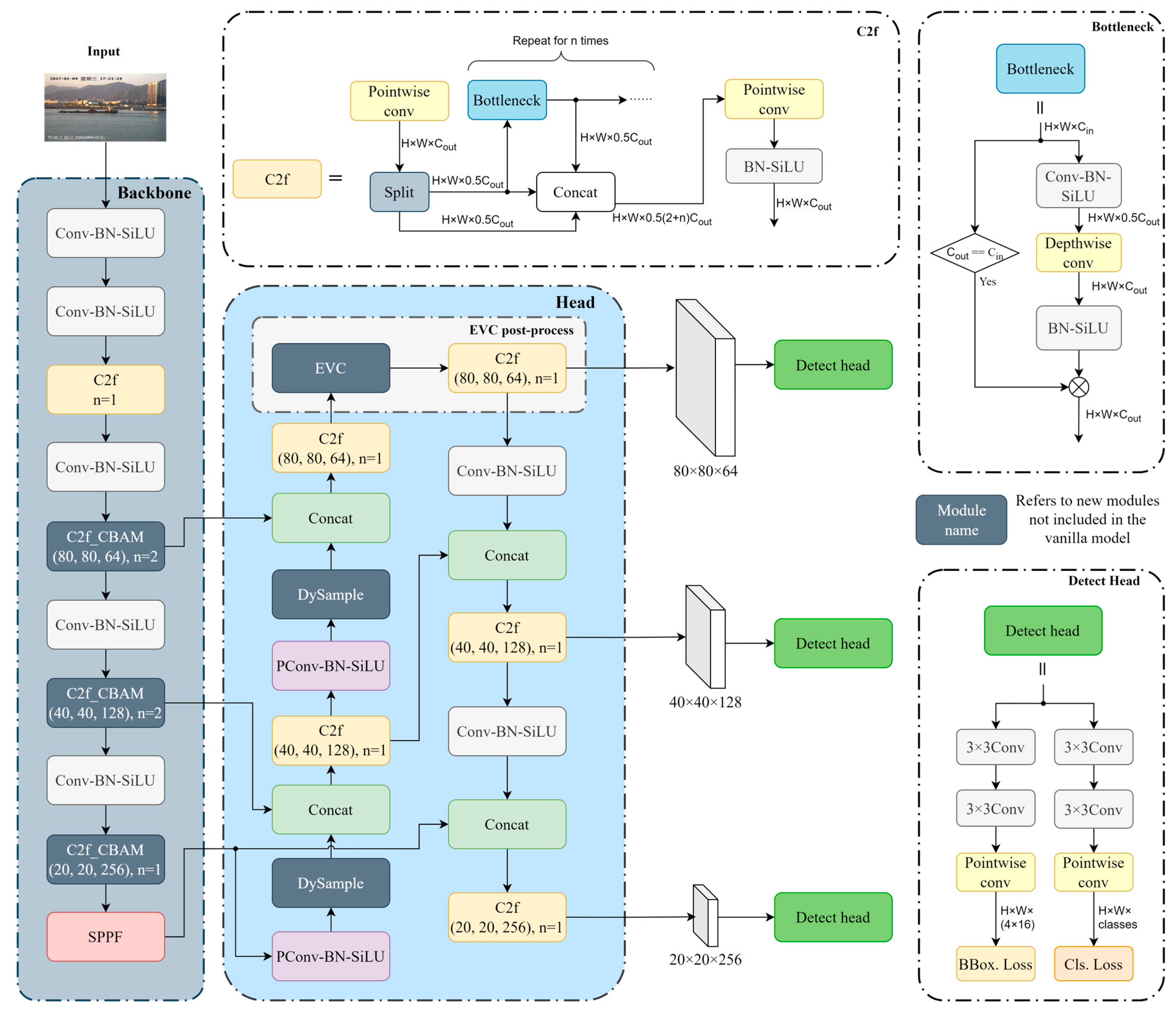
The general structure of YOLO-LPSS is shown in Figure 1. First, some of the C2f modules of the backbone network are added with CBAM, replacing the C2f module at the same location, i.e., C2f_CBAM. C2f_CBAM has the same gradient information flow as C2f, but we apply CBAM only to the deep feature maps of C2f to focus on the features we need, rather than applying CBAM to each module output within the C2f or to C2f outputs to apply CBAM. This structure makes efficient use of the deep features while minimizing the increment in the number of parameters due to the inclusion of the attention mechanism. Then, the DySample up-sample module is introduced in the resample process to replace the original nearest-neighbor interpolation so that the up-sample process takes into account the semantic information of the input feature map and learns how to improve the up-sample strategy based on the feature map. In addition, since the up-sample is performed on high-dimensional feature maps, we partially modified the internal structure of DySample to reduce the computational complexity of the convolution operation. Finally, in the output layer of the resample, the EVC post-processing module was added, which consists of the EVC and C2f modules.
Figure 1.
The general structure of YOLO-LPSS. In the network, the C2f module containing the CBAM attention mechanism is labeled C2f_CBAM, and parameter n of C2f and C2f_CBAM represents the number of iterations of the internal bottleneck or the bottleneck containing the CBAM. Blocks with a black background and white font color refer to new modules not included in the vanilla model. Note that the combination of pointwise convolution [31] (PConv), batch normalization [32] (BN), and Sigmoid Linear Units [33] (SiLU) is abbreviated as PConv-BN-SiLU.
CBAM extracts attention over channels and spatial, but attention extraction based on pointwise convolution [31], pooling, and 7 × 7 large kernel convolution cannot provide pixels with information over longer distances in the same spatial, i.e., each pixel has a limited receptive field. The EVC post-processing module can capture the global dependence on different channels of the feature maps so as to compensate for the drawbacks of CBAM. Meanwhile, EVC can also restore the lost local area information of the deep features so as to enhance the detection accuracy of small targets. Note that we keep the original down-sample process because the feature layer after the EVC post-processing module already has enough small target-oriented semantic information, and adding extra work is not effective in improving the detection accuracy of small target detection.
2.1. Attention Mechanism
The original YOLOv8 can perform feature extraction and target detection well. But, under the requirement of a low parameter count and limited channels, YOLOv8, especially for the nano version, is less able to detect small targets precisely. Therefore, it is necessary to incorporate an attention mechanism into the down-sample process to make the model focus on the important regions in the feature map. In recent years, with the development of self-attention, the Transformer [34] has found a wide range of applications in computer vision due to its ability to capture long-range dependencies. However, the use of self-attention brings many matrix operations to the model. Taking an input matrix of ) as an example, if a single-headed self-attention matrix is computed in pixels, the time complexity is , where each pixel point corresponds to a query and a key, which is far more than the commonly used convolutional. Some works tried to reduce the computation by reducing the rank of the self-attention matrix [35] or by directly reducing the size of the self-attention matrix [36]. But, the final time complexity is still larger than convolution. For the light weight of the model, a convolution-based attention mechanism is used in the proposed model, YOLO-LPSS.
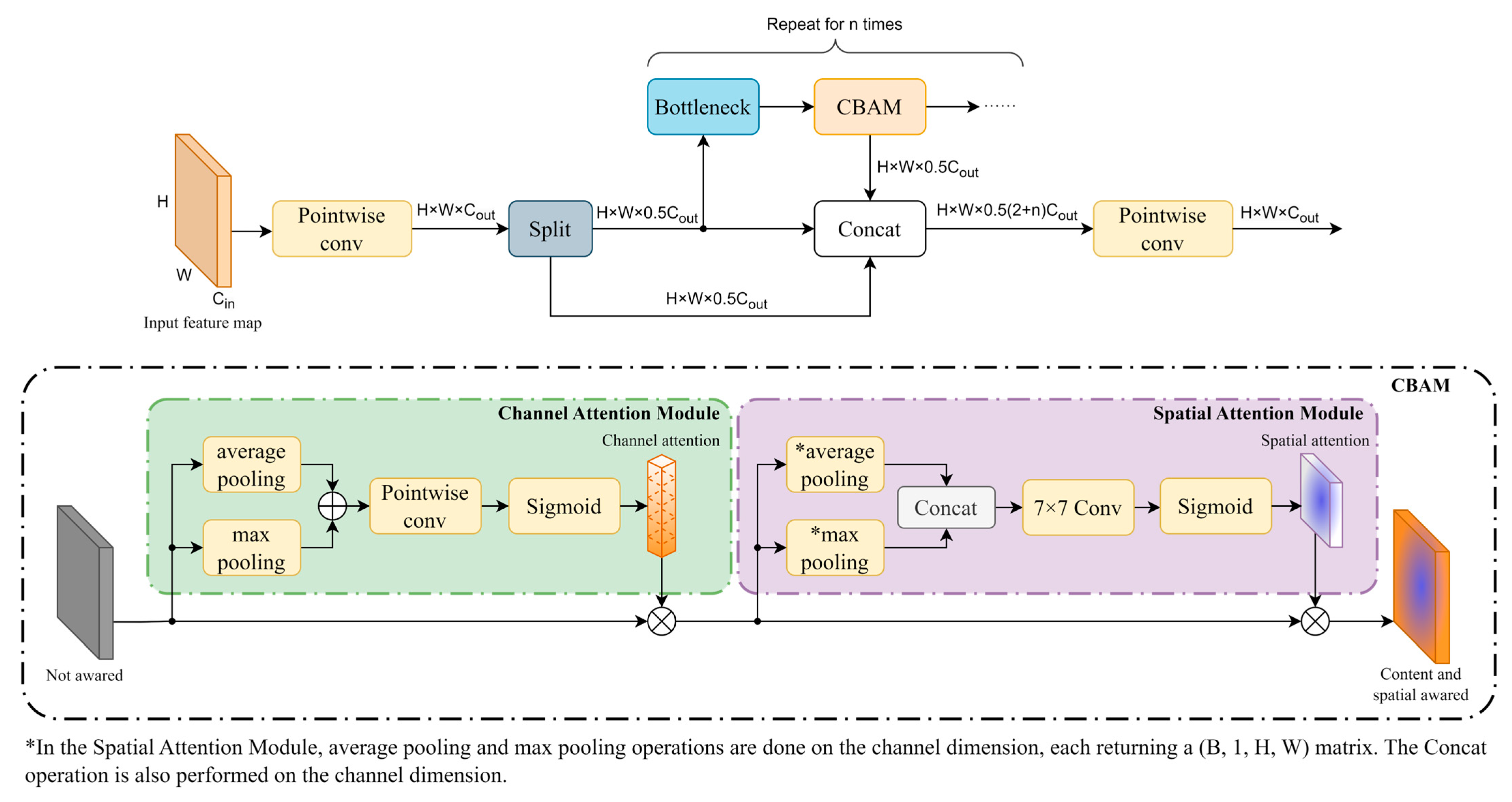
The Convolutional Block Attention Module (CBAM) is currently the most widely used convolution-based attention mechanism. We combined CBAM and C2f to construct the C2f_CBAM module, as shown in Figure 2. In CBAM, the incoming feature maps are first subjected to channel attention, and after obtaining the channel-attention matrix, element-wise multiplication is performed with the original feature maps so that the feature maps have channel attention. Subsequent spatial attention behaves similarly to channel attention, but average pooling and max pooling are changed to be performed in the height and width dimensions of the feature map, and pointwise convolution [31] is replaced with 7 × 7 Same convolution to generate a spatial attention matrix with a large receptive field. The CBAM is computed as follows:
where denotes the sigmoid activation function, represents the pointwise convolution, which is equal to the Same convolution with a 1 × 1 convolution kernel size. represents the Same convolution with a 7 × 7 convolution kernel size. Since channel attention and spatial attention perform different max pooling and average pooling dimensions, the pooling operations performed on the channel dimension and on the two-bit feature maps are labeled as and , respectively. represents the input feature maps and are concatenated in the channel dimension, as opposed to the channel-attention operation of summing over the channel dimension. Note that despite the different shapes of the feature maps output by channel attention and spatial attention, both perform element-wise multiplication and are, therefore, uniformly represented by .
Figure 2.
C2f_CBAM module and CBAM module.
We applied CBAM to the output of the deeper Bottleneck module. As the depth of the neural network increases, the risk of information being lost during transmission increases, so deeper neural networks need to determine “where to focus” to ensure that important information is not lost during forward propagation. The C2f module combines the outputs of the different layers on the network, where shallow outputs do not need to determine the area of focus, and deeper layers need to add an attention mechanism to retain more semantic information. In addition, the number of parameters added by adding CBAM after the bottleneck is 0.02 M, which is 87% less than the approach of adding CBAM directly at the C2f output, drastically reducing the number of parameters while still achieving similar detection results.
2.2. Learnable Up-Sample
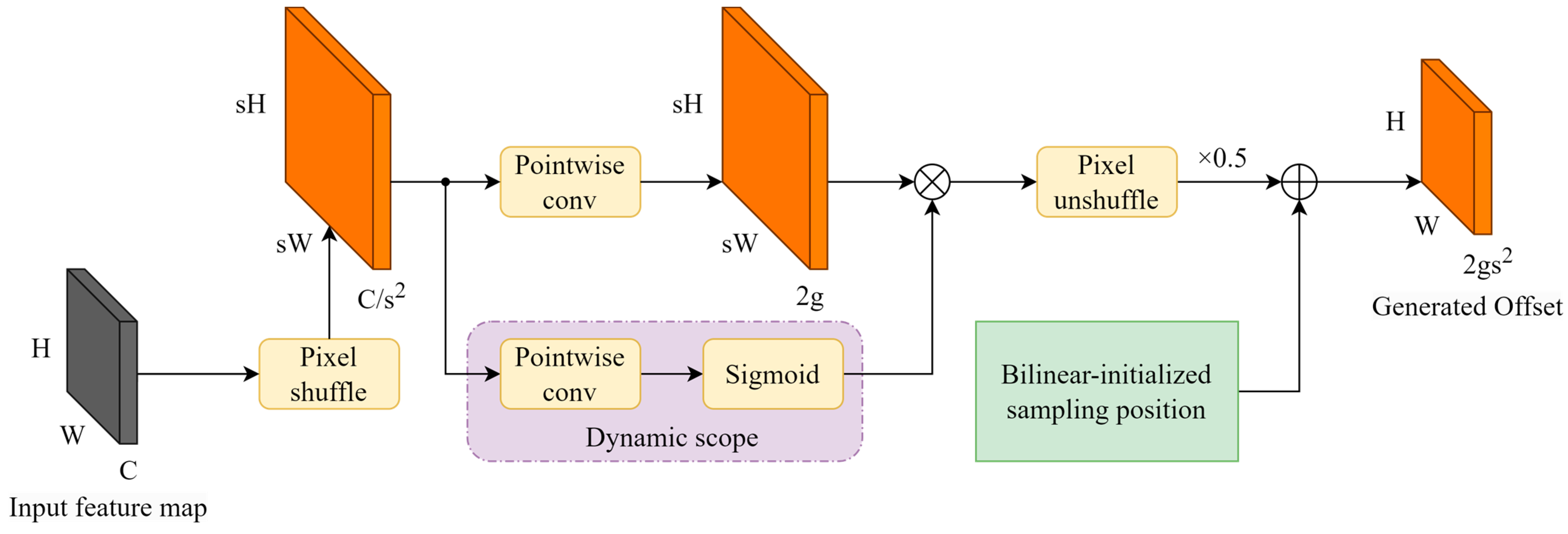
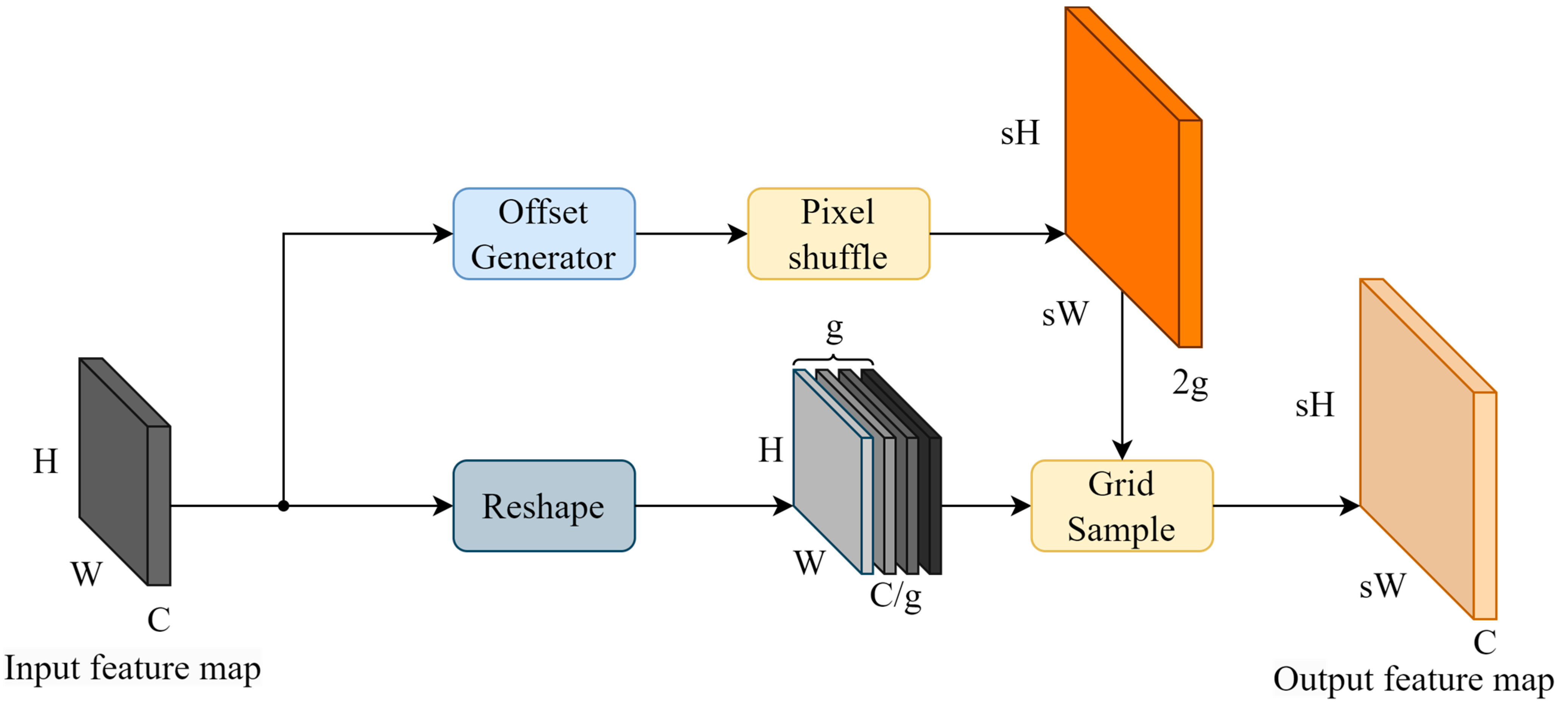
To better exploit the multi-scale features of backbone networks, the feature pyramid networks need to up-sample the deep feature maps and combine the up-sampled feature maps with the high-resolution feature maps. Common feature up-sampling methods include nearest-neighbor interpolation, bilinear interpolation, and joint bilateral up-sample (JBU) [37], which perform well in traditional image processing tasks but ignore the semantic information of the feature maps by using a fixed image processing strategy for the feature maps on each channel. Some up-sample strategies, such as CARAFE [38] and FADE [39], use additional networks to train dynamic convolutional kernels for content-aware up-samples, but the dynamic convolutional kernels rely on the implementation of underlying libraries such as cuDNN, and thus, the models based on this class of strategies are not able to migrate across platforms or perform inference in non-GPU environments. Therefore, YOLO-LPSS adopts an up-sampling method based on point sampling, DySample. Since DySample contains complex dimensional transformations, the changed shape of the feature map during forward propagation is plotted in Figure 3 and Figure 4.

Figure 3.
Structure of the offset generator in DySample and its dimensional change during forward propagation.
Figure 4.
Structure of DySample and its dimensional change during forward propagation.
The core design of DySample is the point offset generator for the input feature map shown in Figure 3. To calculate the offset matrix, the feature map is first subjected to a pixel shuffle [40] to change the shape of to , and then divided into two branches for simultaneous computation. For the first branch, the number of channels is directly transformed into 2g by pointwise convolution; for the second branch, the dynamic scope of the point offset is obtained by the sigmoid activation function after pointwise convolution. The dynamic scope is element-wise multiplied by the output of the first branch to increase the flexibility of the first branch, which is calculated as follows:
where represents the pixel shuffle operation.
When the initialized point samplers are at the same position and the point offsets are equal or 0, the point samplers at this point are equivalent to nearest-neighbor interpolation. To avoid this situation, DySample initializes a constant position for each point sampler by bilinear interpolation, i.e., the bilinear-initialized sampling position in Figure 3. Finally, the channels of the point offset are reduced by pixel unshuffle (PU) [40] (the inverse operation of pixel shuffle), which rearranges the elements in a tensor of shape to . In addition, the bilinear-initialized sampling position is added to obtain the final point offset, calculated as follows:
where represents the pixel unshuffle operation and represents the bilinear-initialized sampling position. To avoid the feature overlap problem caused by the similarity of the output feature values, the output of pixel unshuffle should be multiplied by a feature coefficient (default 0.5) to satisfy the theoretical feature overlap problem to satisfy the theoretical, critical condition of feature overlap and reduce the error caused by feature overlap.
After obtaining the point offset, it is also necessary to perform a pixel shuffle operation to change the shape of the offset to . The grid sample operation [41] of the offset and input feature map is performed to obtain the final up-sampled feature map, which can be expressed as follows:
where denotes the grid sample operation on according to the .
In the original DySample implementation, the offset generator does not include pixel shuffle and pixel unshuffle but directly transforms the channels of the incoming feature map to 2gs2 by pointwise convolution. We found that adding pixel shuffle reduces the number of parameters to and achieves better results, so we used the offset generation method in Figure 4.
Note that when the hyper-parameter is not 1, the shape of the input feature map needs to reshape as , i.e., the feature map is partitioned into groups of in the channel dimension, and the grid sample is performed separately with the guidance of the .
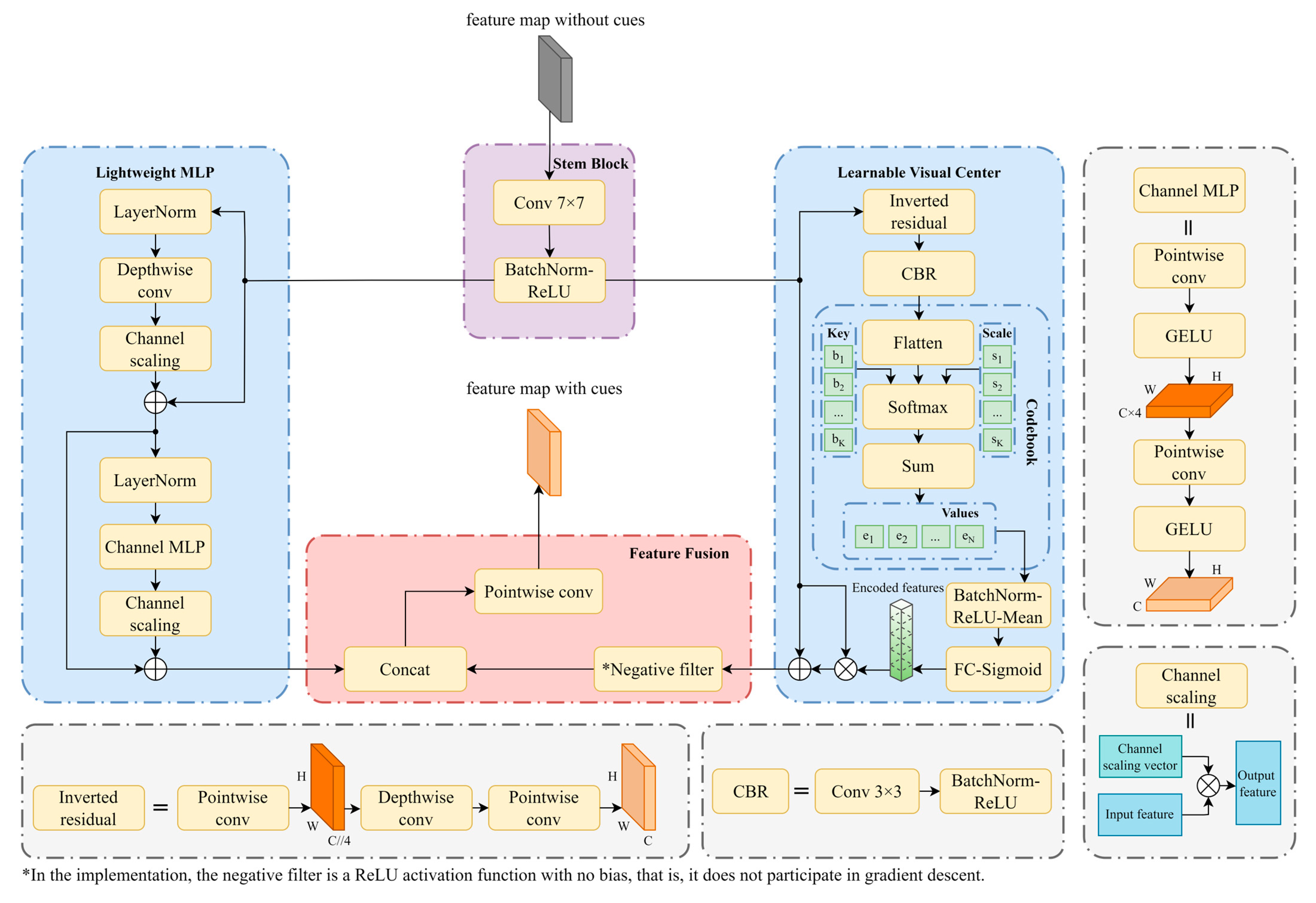
2.3. EVC Post-Process
As mentioned in Section 2.1, traditional attention mechanisms are unable to capture the long-range dependencies in feature maps, and there is still a risk of losing important edge information in forward propagation. Therefore, the EVC post-process module is proposed to solve these two problems. The EVC post-process module consists of the Explicit Visual Center (EVC) module and the C2f module, where the EVC module is shown in Figure 5.
Figure 5.
Structure of EVC and its submodules.
The feature map passed to the EVC is first feature-smoothed by the Stem module, i.e., a module consisting of 7 × 7 Same convolution, batch normalization [32], and ReLU activation function [32] to obtain the feature map . will be passed in parallel into the Lightweight Multi-Layer Perceptrons (LMLP) and the Learnable Visual Center (LVC) to obtain a global-dependence feature map and local corner region feature map. The output feature maps of these two submodules are concatenated and pointwise convolved in the channel dimension to obtain feature maps after integrating the two types of information, computed as follows:
where and represent the LMLP and the LVC submodules, respectively.
2.3.1. LMLP Mechanism
LMLP can be thought of as a cascade of two residual blocks. The first residual block performs layer normalization [42], depthwise convolution [43], and channel scaling [44] operations on the incoming feature map and finally sums with to produce the output , denoted as:
where performs depthwise convolution on the input; that is, for each channel of the input feature map, only one convolution kernel will be convolved with it, which requires fewer convolution kernel parameters than ordinary convolution. represents the layer normalization and is the matrix used in the channel scaling of the first residual block, which updates the parameters during back-propagation with the same channel as .
The second residual block also performs layer normalization on the input feature map and then passes it to the Channel MLP (CMLP) [45], which consists of two pointwise convolutional layers and a GELU activation function. The first pointwise convolution expands the channel dimension of the input feature map by a factor of 4, which is then transformed back to the input channels by the second pointwise convolutional layer through the GELU activation function [33], denoted as:
where and represent two pointwise convolutions, and represents the GELU activation function.
The remainder of the processing is the same as for the first residual block. The output of the CMLP is subjected to the channel scaling operation, which finally gives the output of the LMLP, calculated as:
where is the matrix used in the channel scaling of the second residual block.
In the original LMLP design, each residual block also contains a DropPath [46] module, which achieves regularization by randomly removing elements from the feature map. However, on the feature map with few channels, DropPath would cause an unexpected loss of semantic information, resulting in the model not being able to learn useful features during training. Therefore, we decided to remove the DropPath module from our approach.
2.3.2. LVC Mechanism
LVC firstly preprocesses the input feature map using inverted residual blocks [47] and CBR blocks (the 3 × 3 Same convolution, batch normalization, and ReLU activation function) and then passes them into a built-in coding dictionary called Codebook for the “encoding” operation.
The Codebook consists of two components: (1) a learnable coding dictionary , where K represents the number of “codewords” in the dictionary (default 64); (2) a scaling factor set . For each C-channel vector of the input feature map, a set of scaling factors s sequentially make and map the relative position information , and is calculated as follows:
where is the Euclidean distance between and .
Then, the sum operation is performed on all the relative position information of the kth codeword to obtain the relative position information to the whole feature map. After calculating the relative position information of all the codewords according to Equation (11), batch normalization and ReLU operation are performed on all and are averaged over the dimension K to obtain the global relative position information vector .
where represents batch normalization.
To generate the influence factor for the input feature map, the fully connected (FC) layer and the sigmoid activation function must be passed, projected as a matrix of shape , and then multiplied element-wisely by the input feature map in the channel dimension to obtain the local corner region feature. Finally, the input feature maps are residually connected to the local corner region feature to obtain the output feature maps of LVC.
For similar reasons as in Section 2.3.1, we do not want the LVC to output “where not to focus” due to the limited semantic information of the low-dimensional feature maps. Therefore, we added an additional negative filter, denoted as , to the output of the residual connection. The modified LVC output is shown as follows:
where denotes the fully connected layer, applying a linear transformation to the incoming tensor.
3. Experimental Results and Analysis
3.1. Subsection
The dataset used in this paper is the public version of the ship dataset, Seaships [48], which contains 31,455 images. However, the publicly available version contains only 7000 images. Sea ships contain six categories of ships, with an image resolution of 1920 × 1080, but the percentage of small targets varies significantly for different categories. In our experiment, the dataset is divided into the training set, validation set, and test set in the ratios of 70%, 10%, and 20%.
In Table 1, the bolded items indicate that there are significantly more targets in this category than in other categories. When 5% of the image resolution is used as the threshold for small ships, the percentage of small ships in the fishing boat and passenger ship categories is significantly higher than in the other categories, making the task of detecting targets precisely in these two categories more challenging. Therefore, in the following experiments, we will pay more attention to the detection precision of these two target classes.

Table 1.
Percentage of small ships for all categories in the sea ships.
3.2. Model Evaluation Metrics
In our experiments, we used precision, recall, mean average precision (mAP), parameters, Giga Floating-Point Operations (GFLOPs), and inference time as metrics to evaluate YOLO-LPSS, where precision and recall are calculated as follows:
where TP represents the number of detection boxes that are above a specified confidence threshold and have an IoU greater than a given value with a certain ground truth detection box, and FN represents the number of detection boxes that meet the IoU criteria but are below the confidence threshold. FP consists of two scenarios: (1) the detection boxes that meet the specified confidence threshold, but the IoU with either ground truth is lower than the given value; (2) the detection boxes with low confidence are considered as FP if they satisfy the condition of TP, but conflict with the existing detection boxes.
Average precision (AP) is the area under the precision–recall curve. In theory, AP is obtained by integrating the precision–recall curve as in (16), and the mean average precision (mAP) refers to the mean value of AP in N classes, as in Equation (17).
The stringency of the IoU threshold has a significant effect on AP and mAP, as the IoU determines the allocation of TP and FP detection boxes. By default, the IoU threshold in the AP and mAP calculations is 0.5, i.e., AP50 and mAP50, which is a simple requirement for detection frame accuracy. For this reason, we introduced more demanding metrics: mAP50:95, APPS, and APFB. AP50:95 gradually increases the IoU threshold to 0.95 in steps of 0.05, as in Equation (18), which places higher demands on the model’s precision to generate detection boxes. The mAP50:95 is the average value of AP50:95, which has a calculation process that is equivalent to (17). APPS and APFB are the AP50:95 indicators for two specific classes: passenger ships and fishing boats. As these two classes contain more small boats, we discuss the AP for these two classes separately.
Parameters, Giga Floating Point Operations (GFLOPs), and inference time discuss the complexity of a model in different ways. The parameters refer to the sum of the trainable parameters of the model, such as the convolution kernel; GFLOPs are the number of floating-point operations required by the model during the inference process; and the inference time refers to the average time taken by the model to complete inference process on an image. Note that the number of parameters and GFLOPs do not directly determine the inference time, as the inference process of the model is affected by platform implementation.
3.3. Experimental Results of YOLO-LPSS
All models are trained on an NVIDIA V100 32G GPU with 16 GB of machine RAM and have the same hyperparameters: using the SGD optimizer [49] with an initial learning rate of 0.01, a momentum of 0.937, 200 epochs for training, and the images are preprocessed and resized to 640 × 640 during training. Automatic mixed precision (AMP) is adopted for training, and the inference environment is V100 with FP16 by default.
In terms of the loss function configuration, the (binary cross entropy loss) with a weight of 0.5 is used in the classification branch, while the regression branch consists of two parts: (CIoU loss) with a weight of 7.5 and (distribution focal loss) with a weight of 1.5. In addition to the above loss functions, an L2 regularization with a weight of 0.0005 is added to prevent overfitting. The overall loss function is calculated as follows:
where represents the sum of the squares of all the trainable weights of the model.
The detection results of the original YOLOv8 nano model are shown in Table 2, which performs well enough on most metrics, but YOLOv8 nano performs poorly in the categories where small boats are in the majority.
Table 2.
Detection results of the original YOLOv8 nano.
3.3.1. Ablation Experiments
Because YOLO-LPSS is derived from YOLOv8, the experimental metrics of the models with different structures are shown in Table 3. As shown in Table 3, the application of CBAM in the C2f module effectively improves the AP parameters, including mAP50:95, APFB, and APPS, under high precision requirements with low parametric increase. The addition of the EVC post-process module improves the detection precision for small ships, APFB, and APPS, although there is a small loss of mAP50:95 for all classes and an increase in GFLOPs. After using DySample instead of the conventional up-sample module, the mAP50:95 loss caused by EVC is recovered, with small improvements in APFB and APPS, and the inference time is further reduced to 2.4 ms.
Table 3.
Experimental metrics of the models (including baseline). The green and red values represent the percentage increase or decrease from the baseline model. The best results are marked in bold.
Additionally, the inference time was assessed under conditions of extreme hardware limitations. Due to the incompatibility of Pytorch Aten with FP16 for convolutional operations on CPUs, FP32 inference was performed on the Intel Xeon Gold 6130, and the inference time was recorded. The results are presented in the “CPU FP32 Inference Time (ms)” column of Table 3. It has been observed that LPSS, which necessitates a greater number of matrix operations in the absence of specific CUDA convolutional operators, exhibits slower performance. However, the latency is tolerable within 10 ms when compared to other models.
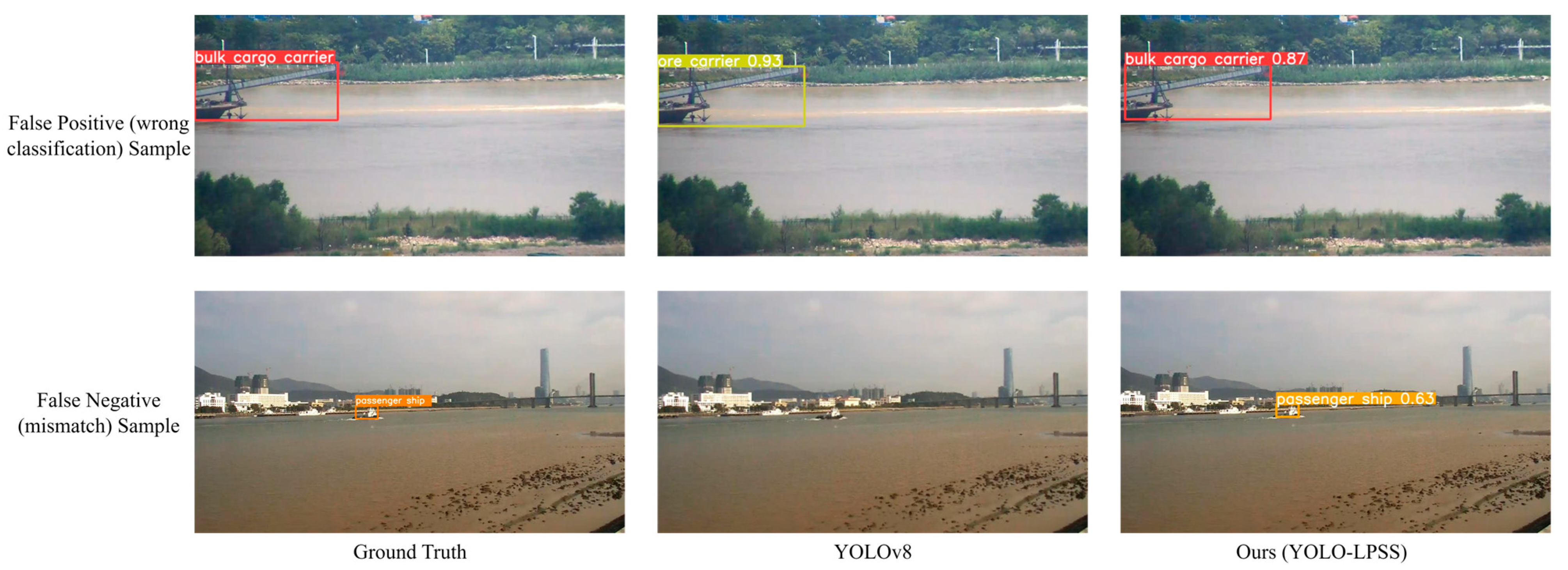
Figure 6 shows the comparison between the capabilities of YOLOv8 and YOLO-LPSS in detecting small ships. It can be seen that YOLO-LPSS has a higher recall and a better classification result for small ship detection tasks with a credible confidence score.

Figure 6.
Comparison of YOLOv8 and YOLO-LPSS in small ship detection.
3.3.2. Paired Sample t-Test
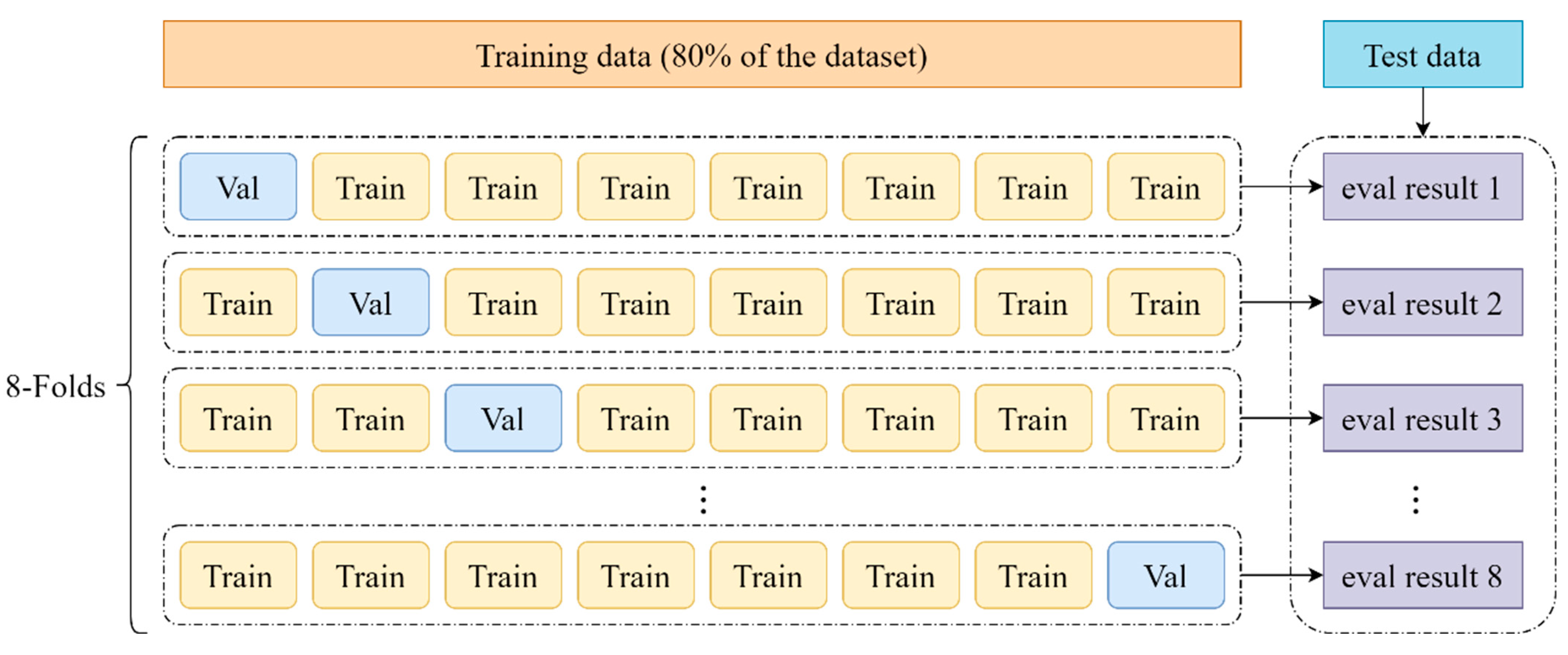
To further demonstrate that the validity of the proposed method is not the result of random errors, an 8-fold cross-validation of YOLO-LPSS and the native YOLOv8 is performed. The paired sample t-test on APPS and APFB is used at a 95% confidence level to test whether the improvement in YOLO-LPSS is statistically significant. It is hypothesized that the outcomes of training with the same samples between the two models are independent and, therefore, can be evaluated using paired sample t-tests. The implementation of statistical significance testing is instrumental in ensuring the reliability of observed improvements, thereby differentiating them from the mere result of random fluctuations.
As shown in Figure 7, all the training data (including the training set and validation set mentioned in Section 3.1) are divided into eight folds. Once training starts, one of the folds is used as the validation set to evaluate the model during training, while the remaining folds are used as the training set in the training process. After training is completed, all models are evaluated on the testing set.
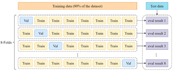
Figure 7.
Process of 8-fold cross-validation.
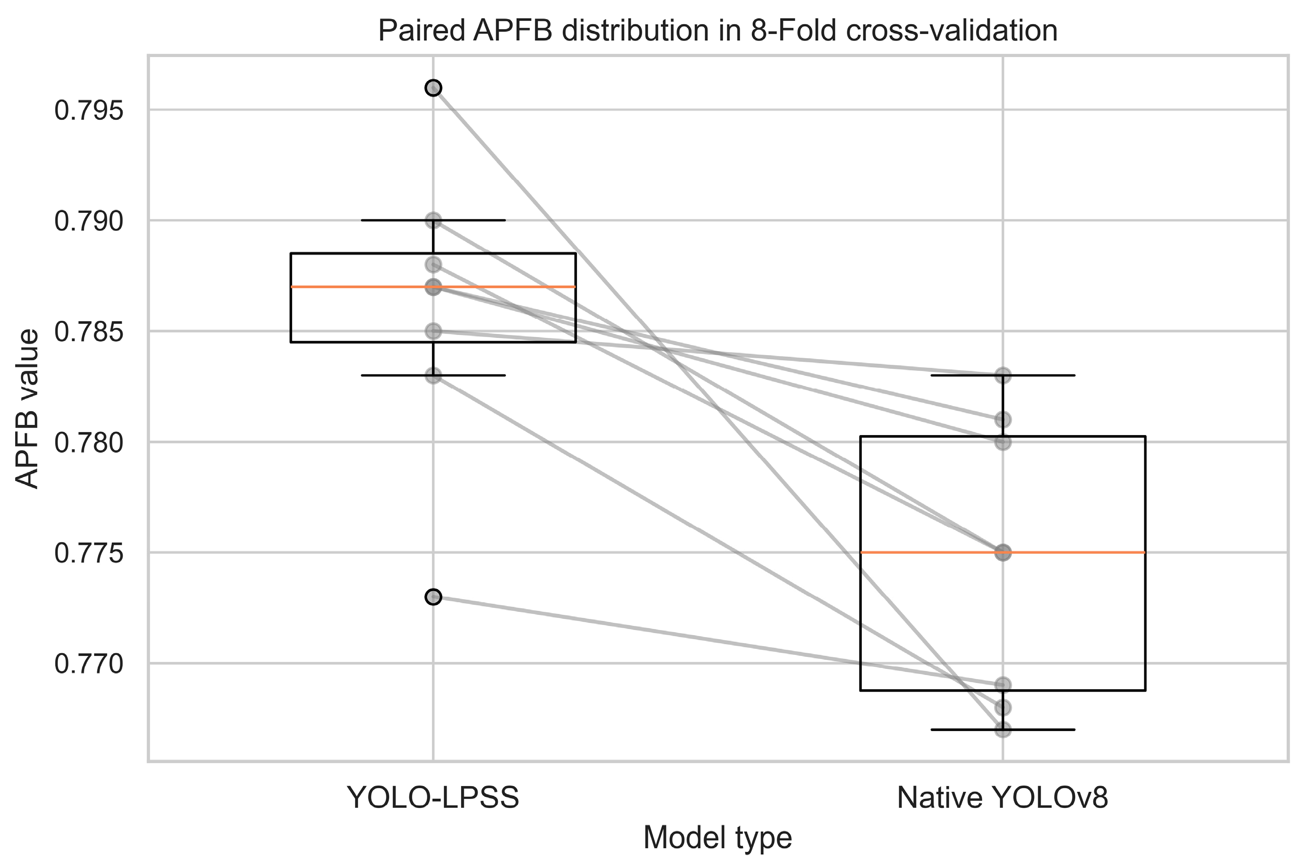
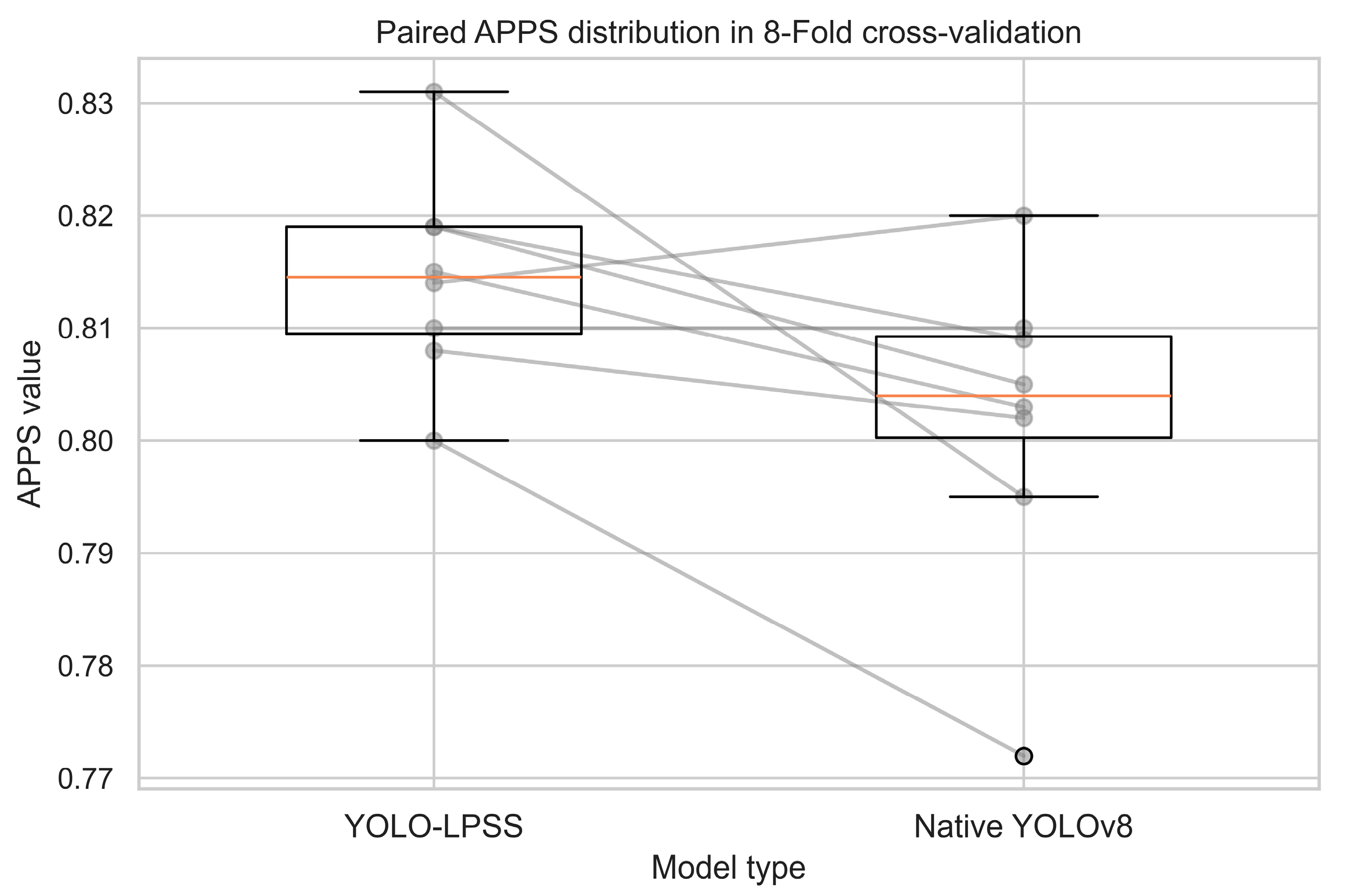
The training data from the same fold of the two models are paired, and the results are shown in Figure 8 and Figure 9, which show that the mean values of YOLO-LPSS are higher than the native YOLOv8 on both APFB and APPS.

Figure 8.
Paired APFB distribution in 8-fold cross-validation.
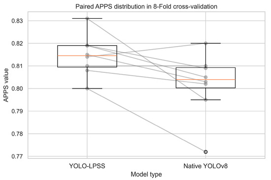
Figure 9.
Paired APPS distribution in 8-fold cross-validation.
In Table 4, the results of the paired sample t-test indicate that the metrics between YOLO-LPSS and the native YOLOv8 are not identically distributed, as both p-values are less than 0.05. Furthermore, a positive t-statistic shows that the YOLO-LPSS metrics are better than the native YOLOv8.
Table 4.
Paired sample t-test on APFB and APPS.
3.3.3. Deep Look at the EVC
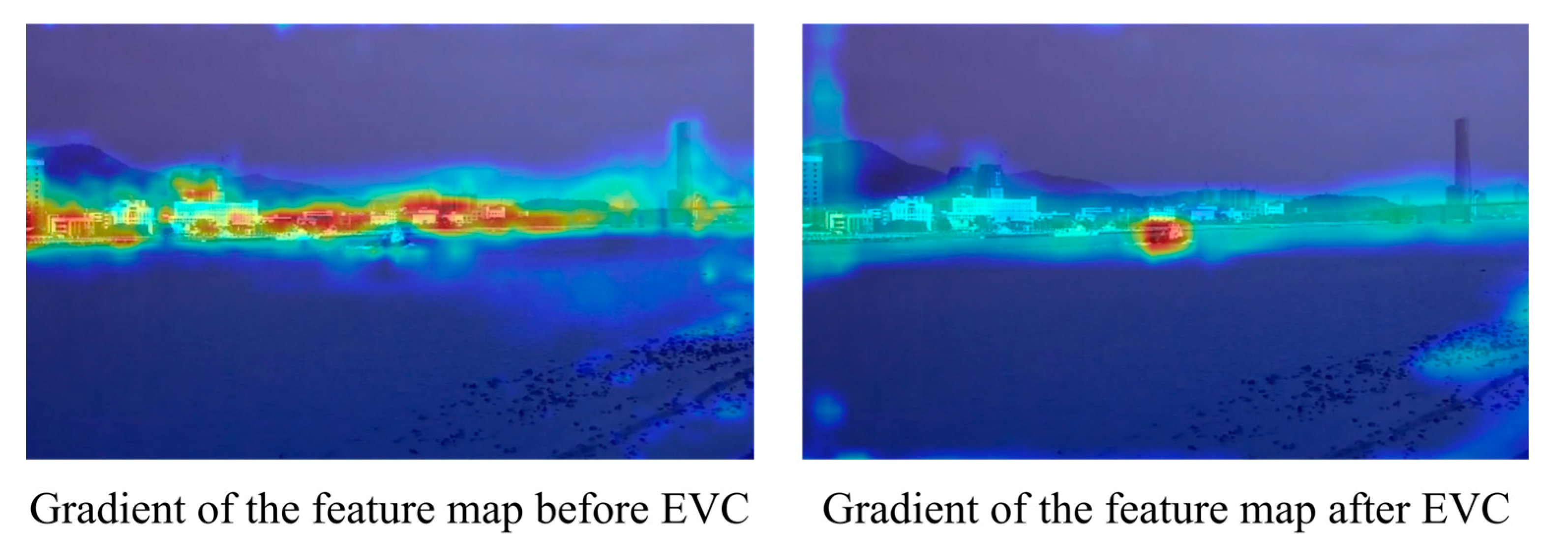
The EVC module has the highest computational demand among all the modules of the model, but the EVC does make the model “focus” on the small boat target. As shown in Figure 10, gradient-weighted class activation mapping (Grad-CAM) [50] is adopted to visualize the gradient of the feature maps before and after the EVC module, and it is obvious that the gradient of the feature maps after EVC processing is higher in the small boat region, i.e., the EVC successfully restores the small boat features lost in the previous feature maps. This raises the question: would reserving more channels for the output of the resample process help the EVC to better restore local area features? If so, how much additional computation would this change require?

Figure 10.
Comparison of the feature map gradient before/after the EVC module.
In this respect, YOLO-LPSS is modified by changing the output channel of the last C2f module in the resample process to 128, i.e., double the normal output and performing the same training. The results of the comparison between the two models are shown in Table 5. After increasing the channels of the output feature map, the number of floating-point operations of the model increases by 10 GFLOPs, which is higher than that of YOLOv8 small, even though the number of parameters of the model increases by only 0.7 M. A comparison of the CPU inference time has also been listed, and the 128 channels version of LPSS takes 54.5 ms longer than the vanilla LPSS. The inference time difference due to the convolutional channel is further amplified in the absence of CUDA convolutional operators and FP16 support.
Table 5.
Comparison of YOLO-LPSS with different numbers of channel inputs to EVC. The bold items denote the best results.
The LVC submodule within the EVC module, or more specifically, the encoding operation of LVC, is the main cause of this phenomenon. In Table 6, we simulate two inputs and passed them to the LVC with full and half-precision, respectively, to analyze the CUDA behavior and time consumption of the LVC in different cases. At full precision, since the encoding operation involves a large number of matrix operations, the number of calls to the CUDA operators varies significantly for different input channels, resulting in a significant difference in the total CUDA time for the two inputs. And at half-precision (FP16), which benefits from a denser data distribution, the number of calls to CUDA operators is the same for different inputs, and the difference in the total CUDA time is reduced, but the total CUDA time corresponding to the input with fewer channels is still smaller than that of the input with more channels.
Table 6.
Research on LVC with different floating-point precision and channels.
3.3.4. Comparisons with Different Models
We compared YOLO-LPSS with the existing classical detection models, such as the Faster R-CNN with a ResNet-50-FPN backbone [7,13,19], YOLOv3 [18], YOLOv5 [51], and RT-DETR [52], and observe their overall performance. In addition to the works mentioned above, we also reproduced recent effective works in the field of ship detection: the multi-scale ship detection model proposed by W. Zhou et al. [23], the YOLOSeaship [1,2], and the SOD-YOLO [53], as shown in Table 7. The training hyperparameters of all models are the same as YOLO-LPSS.
Table 7.
Comparison with existing works. The best results are marked in red bold, and the second best in blue bold.
The faster R-CNN is more difficult to train and requires more training epochs; hence, its poor detection performance on small targets and the application of RoI Align make its GFLOPs much higher than the other models. YOLOv5 and RT-DETR have similar metrics to YOLO-LPSS under high precision requirements, but the number of model parameters and GFLOPs are higher than YOLO-LPSS. SOD-YOLOv8, a model with a focus on small target detection, demonstrates robust performance in APFB and APPS, two metrics that are dominated by small ship targets. However, it exhibits slightly diminished performance in RT-DETR and YOLO-LPSS in the mAP50:95, suggesting that its capacity to detect multi-scale targets is lower than the generic detection model. The results show that YOLO-LPSS has excellent overall performance and accurate detection capability for small ships, while the light weight of the model can meet the demand for real-time detection.
4. Conclusions
In this paper, a lightweight model for accurate detection of small ships is presented. Firstly, the application of the Convolutional Block Attention Module in the C2f module effectively preserves the semantic information of the deep feature maps and improves the detection capability of the model for small targets with a few parameters. In addition, the application of the modified DySample module in the resample process enables the model to have content-aware capability in the up-sample process. Finally, the EVC post-processing module restores local region features in the high-resolution feature maps, further improving the recall of small ship targets. The Seaships dataset was selected to validate the comprehensive performance of YOLO-LPSS and compare it with other detection models. The experimental results show that YOLO-LPSS has better comprehensive performance than other models, combining fast and lightweight detection and high accuracy.
However, we found that some operations in the model, such as grid sampling, have uncertainty and cannot be migrated to other platforms, such as TensorFlow, for inference. Since the grid sampling has no official implementations in Tensorflow and the inference process is specifically designed for CuDNN and CPU backends in Pytorch Aten, it is hard to migrate the pre-trained weight to other platforms. Furthermore, in real-life scenarios, ship detection is often influenced by various weather conditions, lighting environments, or sea conditions. This necessitates the enhancement of the input image (e.g., de-fogging algorithms, low-light enhancement, etc.), i.e., image preprocessing, prior to ship detection, which is not addressed in our work. In future research, we will continue to improve the model’s ability to accurately detect small targets, focus on removing model uncertainty, and integrate effective image preprocessing algorithms to adapt to the challenges of real-life scenarios.
Author Contributions
Conceptualization, L.S. and T.G.; methodology, L.S. and T.G.; software, T.G.; validation, L.S., T.G. and Q.Y.; formal analysis, T.G.; investigation, L.S.; resources, L.S.; data curation, T.G.; writing—original draft preparation, L.S. and T.G.; writing—review and editing, Q.Y.; visualization, T.G.; supervision, Q.Y.; project administration, L.S. and Q.Y.; funding acquisition, Q.Y. All authors have read and agreed to the published version of the manuscript.
Funding
This research was funded by the Key Program for Basic Research of China (Grant number JCKY2023206B026), Liaoning Province General Higher Education Undergraduate Teaching Reform Research Project (Grant 2022166-348).
Data Availability Statement
Data are contained within the article.
Conflicts of Interest
The authors declare no conflicts of interest.
References
- Jiang, X.; Cai, J.; Wang, B.A. Yoloseaship: A lightweight model for real-time ship detection. Eur. J. Remote Sens. 2024, 57, 2307613. [Google Scholar] [CrossRef]
- Cheng, B.; Xu, X.; Zeng, Y.; Ren, J.; Jung, S. Pedestrian trajectory prediction via the Social-Grid LSTM model. J. Eng. 2018, 2018, 1468–1474. [Google Scholar] [CrossRef]
- Corbane, C.; Najman, L.; Pecoul, E.; Demagistri, L.; Petit, M. A complete processing chain for ship detection using optical satellite imagery. Int. J. Remote Sens. 2010, 31, 5837–5854. [Google Scholar] [CrossRef]
- Zhang, Y.; Li, Q.; Zang, F. Ship detection for visual maritime surveillance from non-stationary platforms. Ocean Eng. 2017, 141, 53–63. [Google Scholar] [CrossRef]
- Chen, X.; Hu, R.; Luo, K.; Wu, H.; Biancardo, S.A.; Zheng, Y.; Xian, J. Intelligent ship route planning via an A∗ search model enhanced double-deep Q-network. Ocean Eng. 2025, 327, 120956. [Google Scholar] [CrossRef]
- Simonyan, K.; Zisserman, A. Very deep convolutional networks for large-scale image recognition. arXiv 2014, arXiv:1409.1556. [Google Scholar] [CrossRef]
- He, K.; Zhang, X.; Ren, S.; Sun, J. Deep residual learning for image recognition. In Proceedings of the IEEE Conference on Computer Vision and Pattern Recognition (CVPR), Las Vegas, NV, USA, 27–30 June 2016; pp. 770–778. [Google Scholar]
- Chang, Y.; Anagaw, A.; Chang, L.; Wang, Y.C.; Hsiao, C.; Lee, W. Ship detection based on yolov2 for sar imagery. Remote Sens. 2019, 11, 786. [Google Scholar] [CrossRef]
- Liu, Z.; Hu, J.; Weng, L.; Yang, Y. Rotated region based cnn for ship detection. In Proceedings of the 2017 IEEE International Conference on Image Processing (ICIP), Beijing, China, 17–20 September 2017; pp. 900–904. [Google Scholar]
- Girshick, R.; Donahue, J.; Darrell, T.; Malik, J. Rich feature hierarchies for accurate object detection and semantic segmentation. In Proceedings of the IEEE Conference on Computer Vision and Pattern Recognition, Columbus, OH, USA, 23–28 June 2014; pp. 580–587. [Google Scholar]
- Uijlings, J.R.R.; van de Sande, K.E.A.; Gevers, T.; Smeulders, A.W.M. Selective search for object recognition. Int. J. Comput. Vis. 2013, 104, 154–171. [Google Scholar] [CrossRef]
- Girshick, R. Fast r-cnn. In Proceedings of the IEEE International Conference on Computer Vision (ICCV), Santiago, Chile, 7–13 December 2015; pp. 1440–1448. [Google Scholar]
- Ren, S.; He, K.; Girshick, R.; Sun, J. Faster r-cnn: Towards real-time object detection with region proposal networks. IEEE Trans. Pattern Anal. Mach. Intell. 2017, 39, 1137–1149. [Google Scholar] [CrossRef]
- He, K.; Gkioxari, G.; Dollár, P.; Girshick, R. Mask r-cnn. In Proceedings of the IEEE International Conference on Computer Vision (ICCV), Venice, Italy, 22–29 October 2017; pp. 1703–6870. [Google Scholar] [CrossRef]
- Li, Y.; Xie, S.; Chen, X.; Dollar, P.; He, K.; Girshick, R. Benchmarking detection transfer learning with vision transformers. arXiv 2021, arXiv:2111.11429. [Google Scholar] [CrossRef]
- Liu, W.; Anguelov, D.; Erhan, D.; Szegedy, C.; Reed, S.; Fu, C.; Berg, A.C. Ssd: Single shot multibox detector. In Proceedings of the Computer Vision–ECCV 2016: 14th European Conference, Amsterdam, The Netherlands, 11–14 October 2016; Springer International Publishing: Cham, Switzerland, 2016; pp. 21–37. [Google Scholar]
- Wang, C.; Bochkovskiy, A.; Liao, H.M. Yolov7: Trainable bag-of-freebies sets new state-of-the-art for real-time object detectors. In Proceedings of the 2023 IEEE/CVF Conference on Computer Vision and Pattern Recognition (CVPR), Vancouver, BC, Canada, 17–24 June 2022; pp. 2207–2696. [Google Scholar] [CrossRef]
- Redmon, J.; Farhadi, A. Yolov3: An incremental improvement. arXiv 2018, arXiv:1804.02767. [Google Scholar]
- Lin, T.; Dollár, P.; Girshick, R.; He, K.; Hariharan, B.; Belongie, S. Feature pyramid networks for object detection. In Proceedings of the IEEE Conference on Computer Vision and Pattern Recognition, Honolulu, HI, USA, 21–26 July 2016; pp. 1612–3144. [Google Scholar] [CrossRef]
- Fu, K.; Li, Y.; Sun, H.; Yang, X.; Xu, G.; Li, Y.; Sun, X. A ship rotation detection model in remote sensing images based on feature fusion pyramid network and deep reinforcement learning. Remote Sens. 2018, 10, 1922. [Google Scholar] [CrossRef]
- Ziyu, W.; Tom, S.; Matteo, H.; Hado, H.; Marc, L.; Nando, F. Dueling network architectures for deep reinforcement learning. In Proceedings of the Machine Learning Research, New York, NY, USA, 19–24 June 2016; Maria, F.B., Kilian, Q.W., Eds.; JMLR. 2016; pp. 1995–2003. [Google Scholar]
- Wen, G.; Cao, P.; Wang, H.; Chen, H.; Liu, X.; Xu, J.; Zaiane, O. Ms-ssd: Multi-scale single shot detector for ship detection in remote sensing images. Appl. Intell. 2023, 53, 1586–1604. [Google Scholar] [CrossRef]
- Zhou, W.; Peng, Y. Ship detection based on multi-scale weighted fusion. Displays 2023, 78, 102448. [Google Scholar] [CrossRef]
- Sun, Z.; Dai, M.; Leng, X.; Lei, Y.; Xiong, B.; Ji, K.; Kuang, G. An anchor-free detection method for ship targets in high-resolution sar images. IEEE J. Sel. Top. Appl. Earth Observ. Remote Sens. 2021, 14, 7799–7816. [Google Scholar] [CrossRef]
- Zhang, D.; Wang, C.; Fu, Q. Ofcos: An oriented anchor-free detector for ship detection in remote sensing images. IEEE Geosci. Remote Sens. Lett. 2023, 20, 6004005. [Google Scholar] [CrossRef]
- Feng, C.; Zhong, Y.; Gao, Y.; Scott, M.R.; Huang, W. Tood: Task-aligned one-stage object detection. In Proceedings of the 2021 IEEE/CVF International Conference on Computer Vision (ICCV), Montreal, QC, Canada, 10–17 October 2021; pp. 3490–3499. [Google Scholar]
- Li, X.; Wang, W.; Wu, L.; Chen, S.; Hu, X.; Li, J.; Tang, J.; Yang, J. Generalized focal loss: Learning qualified and distributed bounding boxes for dense object detection. arXiv 2020, arXiv:2006.04388. [Google Scholar] [CrossRef]
- Woo, S.; Park, J.; Lee, J.; Kweon, I.S. Cbam: Convolutional block attention module. arXiv 2018, arXiv:1807.06521. [Google Scholar] [CrossRef]
- Liu, W.; Lu, H.; Fu, H.; Cao, Z. Learning to upsample by learning to sample. arXiv 2023, arXiv:2308.15085. [Google Scholar] [CrossRef]
- Quan, Y.; Zhang, D.; Zhang, L.; Tang, J. Centralized feature pyramid for object detection. IEEE Trans. Image Process. 2023, 32, 4341–4354. [Google Scholar] [CrossRef]
- Chollet, F. Xception: Deep learning with depthwise separable convolutions. arXiv 2016, arXiv:1610.02357. [Google Scholar] [CrossRef]
- Sergey, I.; Christian, S. Batch normalization: Accelerating deep network training by reducing internal covariate shift. In Proceedings of the Machine Learning Research, Lille, France, 6–11 July 2015; Francis, B., David, B., Eds.; JMLR. 2015; pp. 448–456. [Google Scholar]
- Hendrycks, D.; Gimpel, K. Gaussian error linear units (gelus). arXiv 2016, arXiv:1606.08415. [Google Scholar] [CrossRef]
- Vaswani, A.; Shazeer, N.; Parmar, N.; Uszkoreit, J.; Jones, L.; Gomez, A.N.; Kaiser, L.; Polosukhin, I. Attention is all you need. arXiv 2017, arXiv:1706.03762. [Google Scholar] [CrossRef]
- Wang, S.; Li, B.Z.; Khabsa, M.; Fang, H.; Ma, H. Linformer: Self-attention with linear complexity. arXiv 2020, arXiv:2006.04768. [Google Scholar] [CrossRef]
- Dosovitskiy, A.; Beyer, L.; Kolesnikov, A.; Weissenborn, D.; Zhai, X.; Unterthiner, T.; Dehghani, M.; Minderer, M.; Heigold, G.; Gelly, S.; et al. An image is worth 16x16 words: Transformers for image recognition at scale. arXiv 2020, arXiv:2010.11929. [Google Scholar] [CrossRef]
- Kopf, J.; Cohen, M.F.; Lischinski, D.; Uyttendaele, M. Joint bilateral upsampling. ACM Trans. Graph. (ToG) 2007, 26, 96. [Google Scholar] [CrossRef]
- Wang, J.; Chen, K.; Xu, R.; Liu, Z.; Loy, C.C.; Lin, D. Carafe: Content-aware reassembly of features. arXiv 2019, arXiv:1905.02188. [Google Scholar] [CrossRef]
- Lu, H.; Liu, W.; Fu, H.; Cao, Z. Fade: Fusing the assets of decoder and encoder for task-agnostic upsampling. In European Conference on Computer Vision; Springer Nature: Cham, Switzerland, 2022; pp. 231–247. [Google Scholar]
- Shi, W.; Caballero, J.; Huszár, F.; Totz, J.; Aitken, A.P.; Bishop, R.; Rueckert, D.; Wang, Z. Real-time single image and video super-resolution using an efficient sub-pixel convolutional neural network. arXiv 2016, arXiv:1609.05158. [Google Scholar] [CrossRef]
- Jaderberg, M.; Simonyan, K.; Zisserman, A.; Kavukcuoglu, K. Spatial transformer networks. arXiv 2015, arXiv:1506.02025. [Google Scholar] [CrossRef]
- Nair, V.; Hinton, G.E. Rectified linear units improve restricted boltzmann machines. In Proceedings of the 27th International Conference on Machine Learning, Haifa, Israel, 21–24 June 2010; pp. 807–814. [Google Scholar]
- Ba, J.L.; Kiros, J.R.; Hinton, G.E. Layer normalization. arXiv 2016, arXiv:1607.06450. [Google Scholar] [CrossRef]
- Yu, W.; Luo, M.; Zhou, P.; Si, C.; Zhou, Y.; Wang, X.; Feng, J.; Yan, S. Metaformer is actually what you need for vision. arXiv 2021, arXiv:2111.11418. [Google Scholar] [CrossRef]
- Tolstikhin, I.; Houlsby, N.; Kolesnikov, A.; Beyer, L.; Zhai, X.; Unterthiner, T.; Yung, J.; Steiner, A.; Keysers, D.; Uszkoreit, J.; et al. Mlp-mixer: An all-mlp architecture for vision. arXiv 2021, arXiv:2105.01601. [Google Scholar] [CrossRef]
- Larsson, G.; Maire, M.; Shakhnarovich, G. Fractalnet: Ultra-deep neural networks without residuals. arXiv 2016, arXiv:1605.07648. [Google Scholar] [CrossRef]
- Sandler, M.; Howard, A.; Zhu, M.; Zhmoginov, A.; Chen, L. Mobilenetv2: Inverted residuals and linear bottlenecks. arXiv 2018, arXiv:1801.04381. [Google Scholar] [CrossRef]
- Shao, Z.; Wu, W.; Wang, Z.; Du, W.; Li, C. Seaships: A large-scale precisely annotated dataset for ship detection. IEEE Trans. Multimed. 2018, 20, 2593–2604. [Google Scholar] [CrossRef]
- Bottou, L. Large-scale machine learning with stochastic gradient descent. In Proceedings of the 19th International Conference on Computational Statistics, Paris, France, 22–27 August 2010; pp. 177–186. [Google Scholar]
- Selvaraju, R.R.; Cogswell, M.; Das, A.; Vedantam, R.; Parikh, D.; Batra, D. Grad-cam: Visual explanations from deep networks via gradient-based localization. arXiv 2016, arXiv:1610.02391. [Google Scholar] [CrossRef]
- Jocher, G.; Chaurasia, A.; Stoken, A.; Borovec, J.; Kwon, Y.; Michael, K.; Fang, J.; Wong, C.; Yifu, Z.; Montes, D. Ultralytics/yolov5: v6.0—YOLOv5n ‘Nano’ Models, Roboflow Integration, TensorFlow Export, OpenCV DNN Support. Zenodo. 2021. Available online: https://zenodo.org/records/5563715 (accessed on 4 May 2025).
- Zhao, Y.; Lv, W.; Xu, S.; Wei, J.; Wang, G.; Dang, Q.; Liu, Y.; Chen, J. Detrs beat yolos on real-time object detection. arXiv 2023, arXiv:2304.08069. [Google Scholar] [CrossRef]
- Khalili, B.; Smyth, A.W. SOD-YOLOv8—Enhancing YOLOv8 for Small Object Detection in Aerial Imagery and Traffic Scenes. Sensors 2024, 24, 6209. [Google Scholar] [CrossRef]
Disclaimer/Publisher’s Note: The statements, opinions and data contained in all publications are solely those of the individual author(s) and contributor(s) and not of MDPI and/or the editor(s). MDPI and/or the editor(s) disclaim responsibility for any injury to people or property resulting from any ideas, methods, instructions or products referred to in the content. |
© 2025 by the authors. Licensee MDPI, Basel, Switzerland. This article is an open access article distributed under the terms and conditions of the Creative Commons Attribution (CC BY) license (https://creativecommons.org/licenses/by/4.0/).