Mid-Water Ocean Current Field Estimation Using Radial Basis Functions Based on Multibeam Bathymetric Survey Data for AUV Navigation

Abstract

Autonomous Underwater Vehicle (AUV) navigation relies on bottom-tracking velocity from Doppler Velocity Log (DVL) for positioning through dead-reckoning or aiding Strapdown Inertial Navigation System (SINS). In mid-water environments, the distance between the AUV and the seafloor exceeds the detection range of DVL, causing failure of bottom-tracking and leaving only water-relative velocity available. This makes unknown ocean currents a significant error source that leads to substantial cumulative positioning errors. This paper proposes a method for mid-water ocean current estimation using multibeam bathymetric survey data. First, the method models the regional unknown current field using radius basis functions (RBFs) and establishes an AUV dead-reckoning model incorporating the current field. The RBF model inherently satisfies ocean current incompressibility. Subsequently, by dividing the multibeam bathymetric point cloud data surveyed by the AUV into submaps and performing a terrain-matching algorithm, relative position observations among different AUV positions can be constructed. These observations are then utilized to estimate the RBF parameters of the current field within the navigation model. Numerical simulations and experiments based on real-world bathymetric and ocean current data demonstrate that the proposed method can effectively capture the complex spatial variations in ocean currents, contributing to the accurate reconstruction of the mid-water current field and significant improvement in positioning accuracy.

1. Introduction

Autonomous Underwater Vehicles (AUVs) are important tools in oceanographic research, underwater exploration, and environmental monitoring, enabling data collection in regions inaccessible to traditional methods [1,2]. Robust navigation and positioning are essential for AUVs to follow designated trajectories, gather valid scientific data, and return to docking stations.

A fundamental obstacle to underwater AUV navigation is the inaccessibility of Global Navigation Satellite System (GNSS) signals due to the rapid attenuation of electromagnetic waves in water. Consequently, Inertial Navigation Systems (INS), based on dead-reckoning principles, have become the cornerstone of underwater navigation. INS offers the advantage of providing continuous, high-frequency navigation data without reliance on external signals [3]. However, a critical limitation of INS lies in the inherent nature of the Inertial Measurement Unit (IMU). These sensors, while highly sensitive, are susceptible to biases and random errors. These errors, even if initially small, accumulate over time through the integration process inherent in dead-reckoning, leading to a progressive degradation of positional accuracy. This error propagation becomes particularly pronounced during extended underwater missions, significantly impacting the reliability of INS-based navigation alone [4].

Currently, AUV underwater navigation primarily relies on integrated INS/DVL/PS navigation systems. Pressure sensors (PSs) offer high accuracy without cumulative errors, simplifying the three-dimensional navigation problem to a two-dimensional space [5]. Doppler Velocity Logs (DVLs) in the bottom-tracking mode provide accurate absolute velocity measurements without cumulative errors, helping to correct exponentially divergent errors of the INS to a linear divergence state [6]. The core limitation of this integrated navigation approach is that AUV requires continuous DVL bottom-tracking capability, which typically has a maximum effective range of approximately 200 m from the seafloor. When AUVs operate beyond this range, bottom-tracking becomes invalid, making it impossible to obtain absolute velocity information. In such cases, only the velocity relative to the water of the AUV can be measured. When ocean currents are present with unknown velocities, this water-relative velocity becomes insufficient for navigation assistance.

The challenge of AUV navigation in the presence of unknown ocean currents has been addressed through various approaches. Early approaches employed simplified models that treat ocean currents as constant and irrotational. Hegrenaes and Hallingstad [7] presented a state-of-the-art model-aided inertial navigation system (MA-INS) for underwater vehicles under this assumption. Similarly, Wang et al. [8] proposed a SINS/DVL integrated navigation method, with the use of an improved VBAKF algorithm to reduce noise interference, assuming that currents remain constant over short intervals. However, these simplified models inadequately represent the dynamic nature of marine environments, where currents rarely remain static [9].

To better capture current dynamics, Gauss–Markov models have been implemented to characterize spatial and temporal variations in ocean currents [10]. Li et al. [11] proposed an ocean current coefficient estimation method for GNSS/EML/SINS integrated navigation, modeling ocean current velocity as a first-order Gaussian Markov process and using Kalman filter corrections to accurately estimate the current coefficient. Ben et al. [12] introduced an integrated navigation algorithm based on an improved Expected-Mode Augmentation (IEMA) technique for INS/WT-DVL systems, addressing the limitations of using a single ocean current model.

Furthermore, Medagoda et al. [13,14] introduced a layer-based current model that divides the water column into discrete depth layers with constant current velocities within each layer. This approach acknowledges the vertical stratification of ocean currents but neglects horizontal spatial variations. Wang et al. [15] further refined this concept by implementing a hierarchical water velocity estimation method. Yao et al. [16] introduced a staggered grid-based water current-aided SINS/DVL integration solution that improves mid-water navigation by accounting for spatial variations, later enhancing this with a modified smoothing scheme [17].

Recent advancements have focused on more comprehensive current field modeling. Wu et al. [18] developed a cooperative current estimation method using multiple AUVs to collectively map flow fields. Shi et al. [19,20] proposed a framework for cooperative flow field estimation that leverages both relative and absolute motion-integration errors across multiple vehicles. A tree-based distributed method for cooperative flow field estimation, as proposed by He et al. [21], uses a tree structure to allow AUVs to solve nonlinear equations for flow field estimation, requiring only a connected communication network among vehicles. While effective, these multi-vehicle approaches increase operational complexity and cost. For single-AUV operations, Klein et al. [22] proposed a novel approach to estimate platform velocity during complete DVL outages based on past DVL measurements and a motion model. Liu et al. [23] proposed a current compensation technique for SINS/DVL integrated navigation using a radial basis function (RBF) neural network, which predicts ground-relative velocity in real time but requires pre-training.

The radial basis function (RBF) approach has emerged as a powerful mathematical tool for the interpolation and approximation of complex functions across various scientific and engineering domains [24]. Unlike traditional mesh-based methods, RBF offers a meshless framework that can handle scattered data points and complex geometries without requiring structured grids. Kong et al. [25] introduced the use of RBF in combination with Tikhonov-Gaussian regularization to solve the ill-posed problem of reconstructing velocity fields in industrial furnaces. Ng and Leung [26] introduced a method that uses RBFs to reconstruct flow fields and subsequently estimate the Finite-Time Lyapunov Exponent (FTLE) from limited Lagrangian trajectory data.

To address the limitations of existing methods, this paper introduces a novel approach for mid-water ocean current field estimation using an RBF model. Our method uniquely integrates terrain-based relative position constraints, derived from multibeam bathymetric survey data, with the RBF current model. These constraints are obtained through terrain matching techniques, providing observed information about the navigation drift due to ocean currents. By embedding the property of incompressibility into the RBF, our approach better captures spatial variations in current velocity and direction. The RBF model parameters are then optimized using the Levenberg–Marquardt algorithm to minimize the discrepancy between predicted and observed drift, effectively estimating the underlying current field.

The rest of this paper is structured as follows: Section 2 details the methodology, encompassing the problem formulation, the RBF-based ocean current field modeling, the derivation of terrain-based relative position constraints using multibeam bathymetry, and the Levenberg–Marquardt optimization process for RBF parameter estimation. Section 3 presents the results of numerical simulations and experiments based on real-world oceanographic data, validating the effectiveness of the proposed method and comparing its performance against conventional approaches. Section 4 concludes the paper by summarizing the key findings, discussing the limitations of the current study, and outlining directions for future research.

2. Methods

2.1. Problem Formulation

The navigation dynamics of an AUV operating in an underwater environment can be described by a state-space model. The AUV state vector typically includes position, velocity, and attitude information,

$$\mathbf{X}\left(t\right)={\left[x\left(t\right),y\left(t\right),u\left(t\right),v\left(t\right),\psi \left(t\right)\right]}^T$$

(1)

where $\left(x,y\right)$ represents the AUV position in the north–east coordinate frame, $\left(u,v\right)$ denotes the surge and sway velocities in the body frame, and $\psi$ is the heading angle. It should be noted that we define this state vector only in planar ordinate since depth can be accurately obtained with the pressure sensor, and the positions of an AUV are the main concerns in this paper.

The continuous-time kinematic equations governing AUV motion can be expressed as,

$$\dot{x}\left(t\right)=v_x=u\left(t\right)\cos \psi \left(t\right)+v\left(t\right)\sin \psi \left(t\right)$$

(2)

$$\dot{y}\left(t\right)=v_y=u\left(t\right)\sin \psi \left(t\right)-v\left(t\right)\cos \psi \left(t\right)$$

(3)

The DVL is a critical sensor for underwater navigation that measures velocity using the Doppler effect of acoustic signals. The velocity measurement accuracy of a DVL is directly proportional to its operating frequency. Higher operating frequencies provide more precise velocity measurements but result in limited operational range.

In mid-water environments, the altitude of AUV above the seafloor exceeds the DVL maximum detection depth and bottom-tracking capability is lost, as illustrated in Figure 1. The DVL will no longer provide reliable ground-relative velocity information to assist AUV navigation.

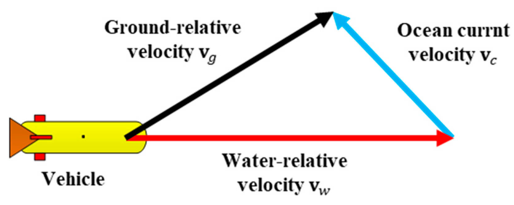
When the bottom-tracking mode is unavailable, the DVL will automatically switch to the water-tracking mode. As illustrated in Figure 2, the ground-relative velocity of the AUV, ${\mathbf{v}}_g\left(t\right)$, is the vector sum of the water-relative velocity, ${\mathbf{v}}_w\left(t\right)$, and the ocean current velocity, ${\mathbf{v}}_c\left(t\right)$, as follows:

$${\mathbf{v}}_g\left(t\right)={\mathbf{v}}_w\left(t\right)+{\mathbf{v}}_c\left(t\right)$$

(4)

where ${\mathbf{v}}_g\left(t\right)$, ${\mathbf{v}}_w\left(t\right)$, and ${\mathbf{v}}_c\left(t\right)$ are the vectors in the navigation frame, ${\mathbf{v}}_w\left(t\right)={\left[v_{w,x}\left(t\right),v_{w,y}\left(t\right)\right]}^T={\left[u_w\left(t\right)\cos \psi \left(t\right)+v_w\left(t\right)\sin \psi \left(t\right),u_w\left(t\right)\sin \psi \left(t\right)-v_w\left(t\right)\cos \psi \left(t\right)\right]}^T$, and $u_w\left(t\right)$ and $v_w\left(t\right)$ are the measured velocities in the DVL water-tracking mode, respectively.

Without loss of generality, the system state is assumed to be observable at initial time instant $t=0$, that is, $\mathbf{p}\left(t_0\right)$ is known. The position of AUV, $\mathbf{p}\left(t\right)={\left[x\right(t),y(t\left)\right)]}^T$, is ideally computed via dead-reckoning as

$$\mathbf{p}\left(t\right)=\mathbf{p}\left(t_0\right)+{\int }_0^t{\mathbf{v}}_g\left(\tau \right)d\tau$$

(5)

However, in practice, since ${\mathbf{v}}_c\left(t\right)$ is unknown, the navigation system approximates positions by integrating only the measured water-relative velocity ${\mathbf{v}}_w\left(t\right)$

$$\widehat{\mathbf{p}}\left(t\right)=\mathbf{p}\left(t_0\right)+{\int }_0^t{\mathbf{v}}_w\left(\tau \right)d\tau$$

(6)

This discrepancy between the estimated position $\widehat{\mathbf{p}}\left(t\right)$ and the true position $\mathbf{p}\left(t\right)$ represents the positioning error due to uncompensated ocean currents as

$$\mathbf{e}\left(t\right)=\mathbf{p}\left(t\right)-\widehat{\mathbf{p}}\left(t\right)={\int }_0^t{\mathbf{v}}_c\left(\tau \right)d\tau$$

(7)

This error accumulates over time and can significantly impact navigation accuracy during long-endurance underwater missions.

2.2. Ocean Current Field Modeling with RBF

To accurately model the ocean current field, we start with the Navier–Stokes equations from computational fluid dynamics, coupled with the mass conservation law. The mathematical expression of the ocean current dynamic model is shown as

$${\displaystyle \frac{\partial \rho }{\partial t}}+\nabla ·\left(\rho \mathbf{V}\right)=0$$

(8)

where $\mathbf{V}$ represents the ocean current velocity field, $\nabla$ denotes the gradient operator, $\rho$ represents fluid density, and $t$ represents time. This equation indicates that within a unit time, the net inflow and outflow in a fluid motion region are equal.

In the study of dynamic oceanography, ocean currents can be modeled as incompressible flows, meaning that density variations are negligible. While density in the ocean does depend on temperature and salinity, these variations are sufficiently small in mid-to-deep ocean currents. This simplification allows us to treat $\rho$ as a constant, i.e., $d\rho /dt=0$. Furthermore, considering that the mid-to-deep ocean currents of interest are primarily dominated by geostrophic flow, which exhibits relatively slow variations within the spatiotemporal scales of AUV operations, we can reasonably assume a time-invariant flow field. Consequently, Equation (8) simplifies to

$$\nabla ·\mathbf{V}={\displaystyle \frac{\partial u}{\partial x}}+{\displaystyle \frac{\partial v}{\partial y}}=0$$

(9)

Based on the potential flow theory [27,28] and the associated assumption of the Laplace equation [29], the velocity field is expressed as the gradient of a velocity potential function $\varphi \left(x,y\right)$, as

$${\mathbf{v}}_c=\left[\begin{array}{c}{v}_{c,x}\\ v_{c,y}\end{array}\right]=\left[\begin{array}{c}{\displaystyle \frac{\partial \varphi \left(x,y\right)}{\partial y}}\\ -{\displaystyle \frac{\partial \varphi \left(x,y\right)}{\partial x}}\end{array}\right]$$

(10)

Radial basis functions (RBFs) offer a versatile, mesh-free approach for representing complex, spatially varying functions [30]. RBFs have properties of universal approximation and best approximation, which also are widely used for function approximation. Common RBF types include Gaussian, multiquadric, and thin-plate spline functions, each offering different interpolation characteristics suitable for various applications [31]. In this study, we use the Gaussian RBF as the potential function to model the ocean current field. The general form of RBF can be written as follows:

$$\varphi \left(\mathbf{p}\right)=\sum _{i=1}^N{\omega }_i\phi \left(‖\mathbf{p}-{\mathbf{c}}_i‖\right)=\sum _{i=1}^N{\omega }_{i}exp\left(-{\displaystyle \frac{{‖\mathbf{p}-{\mathbf{c}}_i‖}^2}{2{\left({\sigma }_i\right)}^2}}\right)$$

(11)

where $\mathbf{p}={\left[x,y\right]}^T$ denotes the position in the ocean current field; $\phi \left(‖\mathbf{p}-{\mathbf{c}}_i‖\right)$ denotes RBF; $N$ denotes the number of RBFs; the subscript $i$ denotes the $i$-th basis function; and ${\omega }_i$, ${\mathbf{c}}_i={\left[c_{i,x},c_{i,y}\right]}^T$, and ${\sigma }_i$ are the weight, center, and width of the $i$-th RBF, respectively.

Physically, the RBF model works by placing center points in the ocean current field and combining their local effects, $\phi \left(‖\mathbf{p}-{\mathbf{c}}_i‖\right)$, to describe the velocity distribution. Each term ${\omega }_i\phi \left(‖\mathbf{p}-{\mathbf{c}}_i‖\right)$ represents a velocity effect starting from ${\mathit{c}}_{\mathit{i}}$, with ${\omega }_i$ controlling its strength of the effect, ${\mathbf{c}}_i$ setting the location, and ${\sigma }_i$ determining the width of the effect reaches.

By substituting Equation (11) into Equation (10), we derive the ocean current as

$${\mathbf{v}}_c\left(\mathbf{p},\mathsf{\alpha }\right)=\left[\begin{array}{c}{v}_{c,x}\\ v_{c,y}\end{array}\right]=\left[\begin{array}{c}-{\displaystyle \sum _{i=1}^N}{\displaystyle \frac{{\omega }_i\left(y-c_{i,y}\right)}{{{\sigma }_i}^2}}exp\left(-{\displaystyle \frac{{‖\mathbf{p}-{\mathbf{c}}_i‖}^2}{2{{\sigma }_i}^2}}\right)\\ {\displaystyle \sum _{i=1}^N}{\displaystyle \frac{{\omega }_i\left(x-c_{i,x}\right)}{{{\sigma }_i}^2}}exp\left(-{\displaystyle \frac{{‖\mathbf{p}-{\mathbf{c}}_i‖}^2}{2{{\sigma }_i}^2}}\right)\end{array}\right]$$

(12)

We define each RBF parameter as ${\mathsf{\alpha }}_{\mathit{i}}=\left[{{\omega }_i,c}_{i,x},c_{i,y},{\sigma }_i\right]$, and the parameters of the ocean current field model as $\mathsf{\alpha }={\left[{\mathsf{\alpha }}_1,\dots ,{\mathsf{\alpha }}_{\mathit{i}},\dots ,{\mathsf{\alpha }}_N\right]}^T$. Equation (10) means that once the parameters $\mathsf{\alpha }$ are determined, the ocean current field can be reconstructed. Furthermore, the ocean current field consistently satisfies the incompressible flow property expressed in Equation (9), namely,

$$\nabla ·\mathbf{V}={\displaystyle \frac{{\partial }^2\varphi \left(\mathbf{p}\right)}{\partial y\partial x}}-{\displaystyle \frac{{\partial }^2\varphi \left(\mathbf{p}\right)}{\partial x\partial y}}=0$$

(13)

Therefore, the central problem addressed in this study is the estimation and optimization of all the RBF parameters $\mathsf{\alpha }$ to accurately capture the characteristics of a given ocean current field. This parameter estimation problem can be framed as an optimization problem, where the objective is to find the set of parameters that minimizes the discrepancy between the predicted velocity field from the RBF model and the measured velocity.

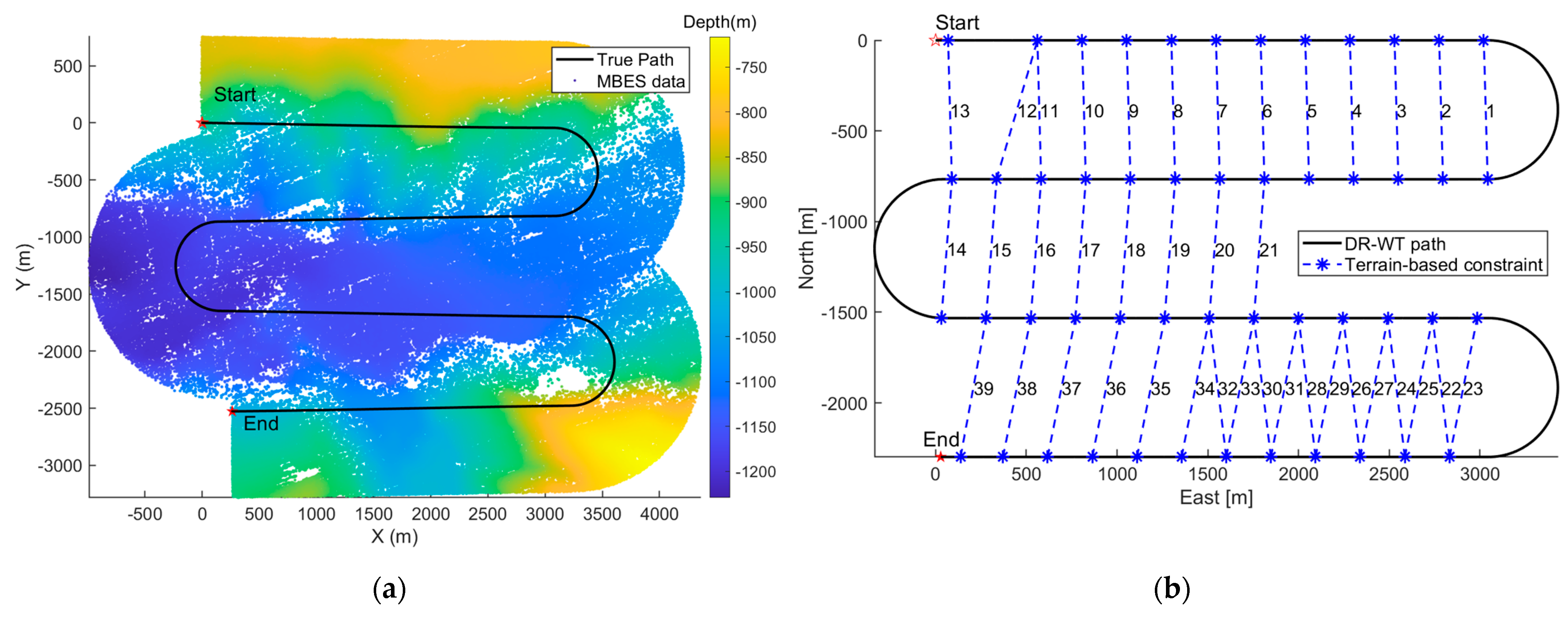
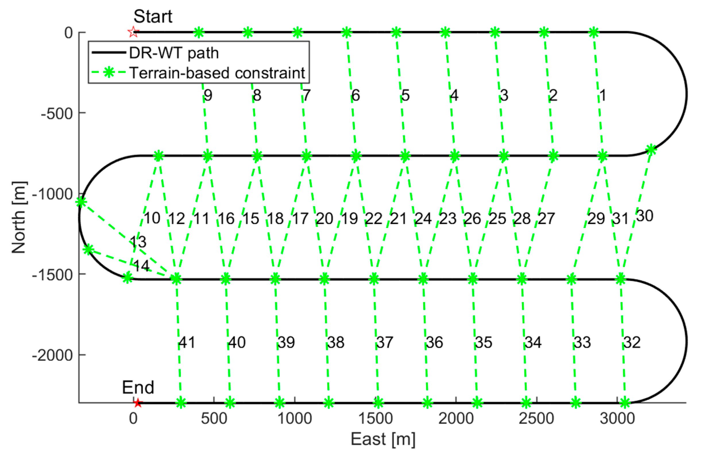
2.3. Terrain-Based Relative Position Constraints Based on MBES

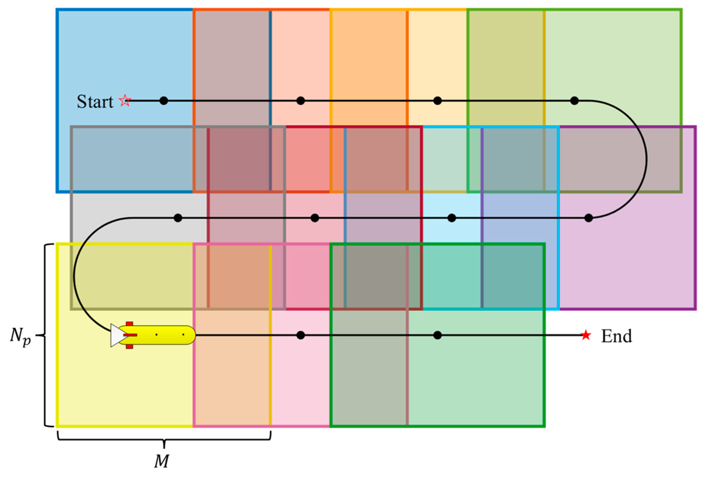
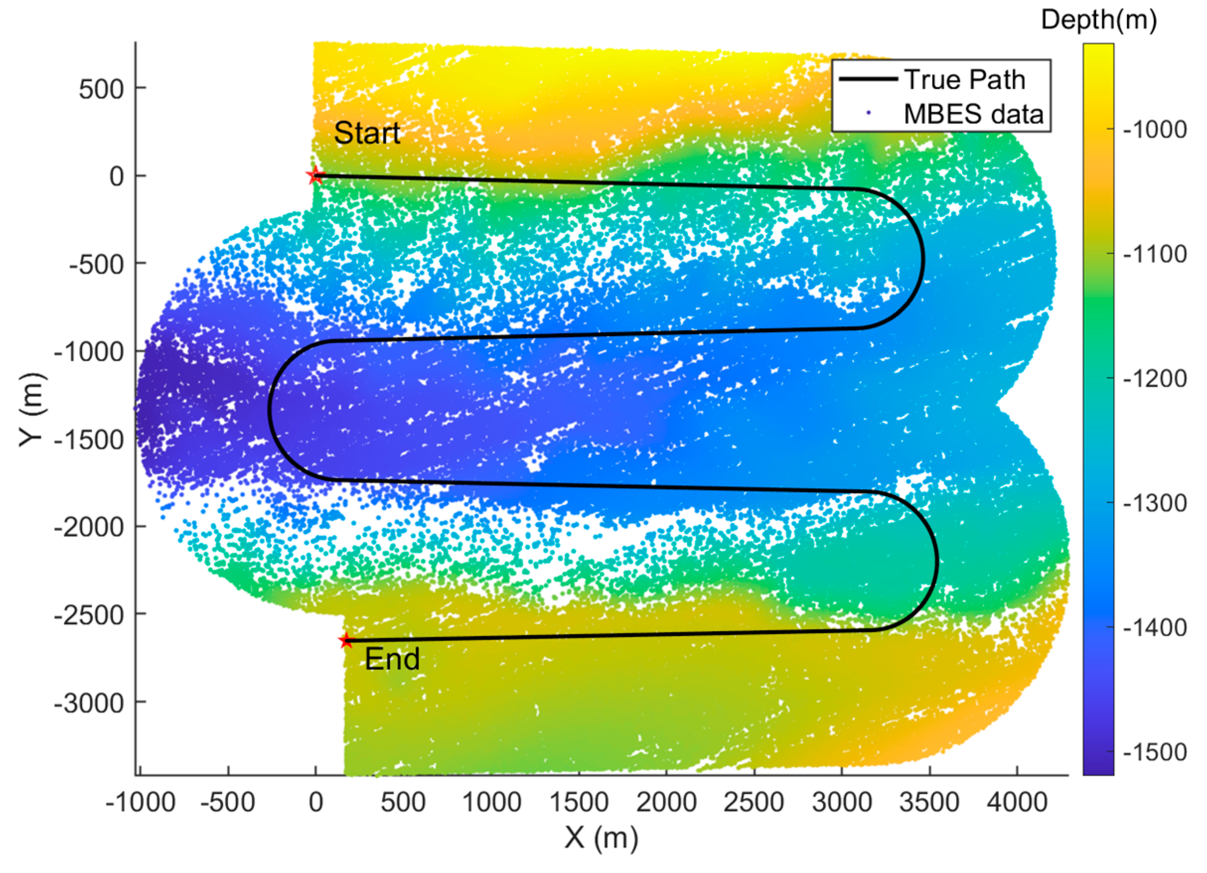
In underwater environments, the AUV equipped with multibeam echo sounders (MBESs) collects bathymetric data along survey lines, generating submaps of the seafloor to determine their relative positions based on terrain matching. The spatial arrangement of survey lines is a critical factor in ensuring both complete seafloor coverage and the robustness of navigation adjustments. Line spacing is designed to achieve a minimum of 25% overlap between adjacent MBES swaths, with an optimal target of 50% overlap [32]. This deliberate overlap provides numerous opportunities for detecting relative position constraints between submaps collected at different times during the mission, as illustrated in Figure 3.

The MBES collects bathymetric data in the form of point clouds, with each ping producing a line-shaped terrain profile perpendicular to the AUV trajectory. For a single ping, the bathymetric point cloud can be expressed as

$$P=\left\{\left(x_i,y_i,z_i\right)|i=\mathrm{1,2},\dots ,N_P\right\}$$

(14)

where $N_P$ is the number of depth points in the ping, $\left(x_i,y_i\right)$ denotes the horizontal coordinates of the i-th point, and $z_i$ corresponds to the measured depth value.

Assuming $M$ consecutive pings are used to construct a submap, the point cloud model can be expressed as

$$S=\bigcup _{k=1}^M{P}_k=\left\{\left(x_j,y_j,z_j\right)|j=\mathrm{1,2},\dots ,N_s\right\}$$

(15)

where $N_s=M\times N_P$ represents the total number of depth points in the submap $S$.

To detect relative position constraints between overlapping submaps in underwater terrain matching, the point-to-plane Iterative Closest Point (ICP) algorithm is used to align bathymetric point clouds obtained from the MBES. Different from the conventional point-to-point ICP, this method minimizes the perpendicular distance from source points to the tangent planes of the target surface, aligning more effectively with the geometric constraints of continuous seafloor topography.

Given a source submap $S_p$ and a target submap $S_q$ with potential overlap, the point-to-plane ICP algorithm iteratively computes the rigid transformation matrix $\mathbf{T}=\left[\mathbf{R}|\mathbf{t}\right] \mathrm{t}\mathrm{o} \mathrm{a}\mathrm{l}\mathrm{i}\mathrm{g}\mathrm{n} S_p \mathrm{a}\mathrm{n}\mathrm{d} S_q$, where $\mathbf{R}$ is the rotation matrix and $\mathbf{t}$ is the translation vector. The ICP algorithm begins by establishing point correspondences between $S_p$ and $S_q$ via a nearest-neighbor search. The alignment is optimized by minimizing the following objective function iteratively, as

$$E\left(\mathbf{R},\mathbf{t}\right)=\sum _{i=1}^{N_s}{‖\left(\mathbf{R}{\mathbf{p}}_{\mathit{i}}+\mathbf{t}-{\mathbf{q}}_{\mathit{i}}\right)·{\mathbf{n}}_i‖}^2$$

(16)

where ${\mathbf{p}}_{\mathit{i}}\in S_p$, ${\mathbf{q}}_{\mathit{i}}\in S_q$, ${\mathbf{n}}_i$ represents the normal vector at target ${\mathbf{q}}_{\mathit{i}}$.

Iterations continue until convergence, determined by a predefined threshold or maximum iteration limit. Once the optimal transformation ${\mathbf{T}}^{\mathit{*}}=\left[{\mathbf{R}}^{\mathit{*}}|{\mathbf{t}}^{\mathit{*}}\right]$ is obtained, $S_p$ is transformed to $S_p^{\prime }$, computed as

$$S_p^{\prime }={\mathbf{R}}^{\mathit{*}}{S}_p+{\mathbf{t}}^{\mathit{*}}$$

(17)

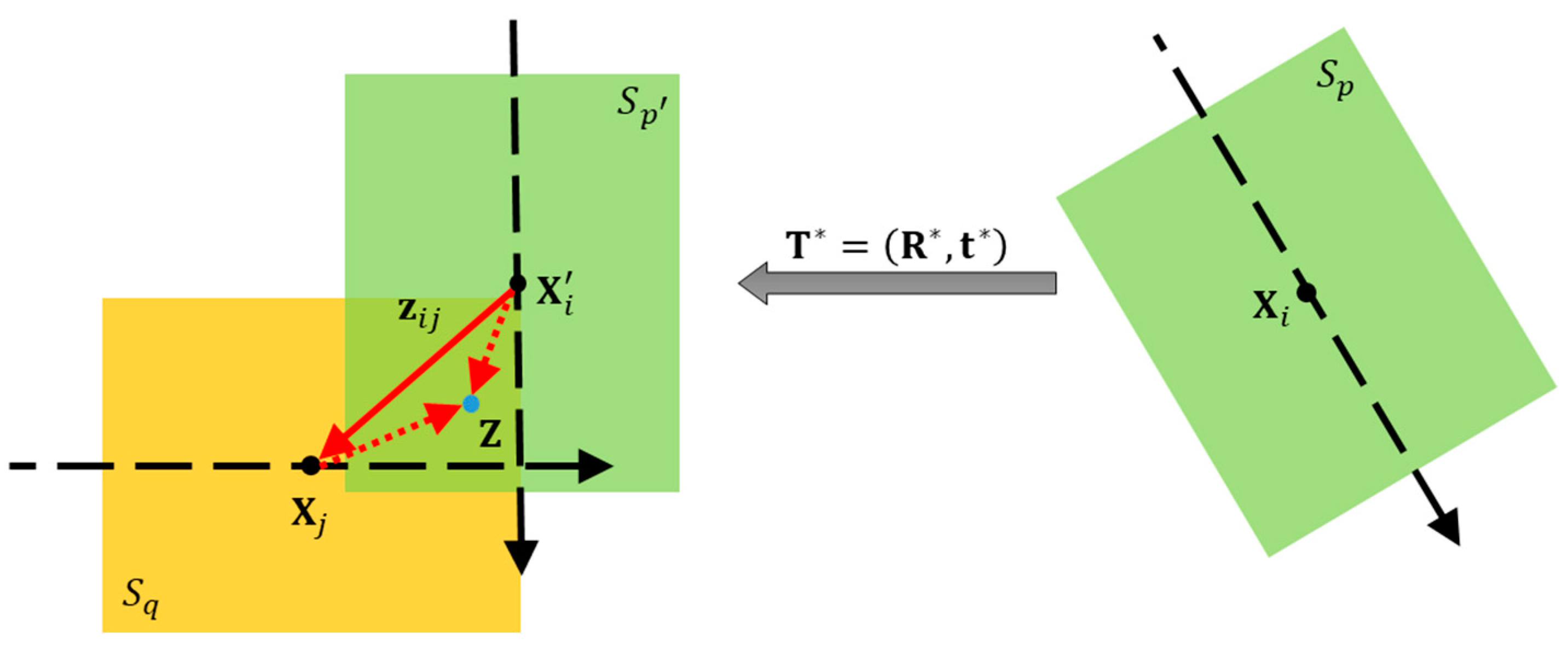
As illustrated in Figure 4, a relative position constraint based on terrain matching can be formulated as,

$${\mathbf{z}}_{ij}=g\left(S_p,S_q\right)=\left(\mathbf{Z}-{\mathbf{X}}_i\right)+\left({\mathbf{X}}_j-\mathbf{Z}\right)$$

(18)

where $g$(⋅) denotes the ICP algorithm; ${\mathbf{X}}_i$ and ${\mathbf{X}}_j$ are the centroids of submaps $S_p^{\prime }$ and $S_q$, respectively; and $\mathbf{Z}$ is the centroid of the overlapped region of $S_p^{\prime }$ and $S_q$.

2.4. Levenberg–Marquardt Optimization for RBF Parameter Estimation

Building upon the terrain-based relative position constraints established in Section 2.3, this section describes the optimization process for estimating RBF parameters that characterize the ocean current field affecting AUV navigation.

The estimation of RBF parameters, denoted as $\mathsf{\alpha }$, is formulated as a nonlinear least-squares problem. The objective is to minimize the discrepancy between the predicted AUV drift due to the estimated ocean current field and the observed drift inferred from terrain-based relative position constraints.

For a relative position constraint between AUV poses at times $t_i$ and $t_j$, the measured relative position displacement is denoted as

$$∆{\mathbf{p}}_{ij}={\mathbf{p}}_j-{\mathbf{p}}_i={\mathbf{z}}_{ij}$$

(19)

The predicted relative displacement based on the ocean current model is expressed as

$$∆{\widehat{\mathbf{p}}}_{ij}={\widehat{\mathbf{p}}}_j-{\widehat{\mathbf{p}}}_i={\int }_{t_i}^{t_j}\left({\mathbf{v}}_w\left(t\right)+{\mathbf{v}}_c\left(\mathbf{p}\left(t\right),\mathsf{\alpha }\right)\right)dt$$

(20)

where ${\mathbf{v}}_c\left(\mathbf{p},\mathsf{\alpha }\right)$ represents the ocean current velocity at position $\mathbf{p}$ parameterized by $\mathsf{\alpha }$.

The cost function is defined to quantify the discrepancy between the measured displacement $∆{\mathbf{p}}_{ij}$ and the predicted displacement $∆{\widehat{\mathbf{p}}}_{ij}$ across all the $N_L$ relative position constraints identified in the terrain matching algorithm, as

$$E\left(\mathsf{\alpha }\right)=\sum _{l=1}^{N_L}{‖∆{\mathbf{p}}_{ij}-∆{\widehat{\mathbf{p}}}_{ij}‖}^2=\sum _{l=1}^{N_L}{‖{\mathbf{z}}_{ij}-{\int }_{t_i}^{t_j}\left({\mathbf{v}}_w\left(t\right)+{\mathbf{v}}_c\left(\mathbf{p}\left(t\right),\mathsf{\alpha }\right)\right)dt‖}^2$$

(21)

where $\mathsf{\alpha }$ represents the RBF parameters set to be optimized, and $l$ indexes each terrain-based relative position constraint.

The Levenberg–Marquardt (LM) algorithm is employed to minimize the cost function $E\left(\mathsf{\alpha }\right)$ by iteratively adjusting the RBF parameters $\mathsf{\alpha }$. The LM method combines the steepest descent and Gauss–Newton approaches, offering both stability and efficiency for nonlinear optimization problems.

The LM algorithm iteratively updates the parameters, starting with an initial estimate ${\mathsf{\alpha }}_0$. At each iteration $k$, $\mathsf{\alpha }$ is updated as follows:

$${\mathsf{\alpha }}_{k+1}={\mathsf{\alpha }}_k+{∆\mathsf{\alpha }}_k$$

(22)

where ${∆\mathsf{\alpha }}_k$ is the update increment which is obtained by solving the following system of linear equations:

$$\left({\mathbf{J}}_k^{\mathrm{T}}{\mathbf{J}}_k+{\lambda }_k\mathbf{I}\right){∆\mathsf{\alpha }}_k=-{\mathbf{J}}_k^{\mathrm{T}}\mathbf{r}\left({\mathsf{\alpha }}_k\right)$$

(23)

where $\mathbf{r}=∆{\mathbf{p}}_{ij}-∆{\widehat{\mathbf{p}}}_{ij}$ is the residual vector representing the error between observed and predicted relative displacements, $\mathbf{r}\left({\mathsf{\alpha }}_k\right)$ is the residual vector evaluated at ${\mathsf{\alpha }}_k$, ${\mathbf{J}}_k$ is the Jacobian matrix of $\mathbf{r}\left({\mathsf{\alpha }}_k\right)$ which contains the partial derivatives of the residuals with respect to each parameter in $\mathsf{\alpha }$, and ${\lambda }_k$ is the adaptive damping factor that controls the balance between the steepest descent and Gauss–Newton methods during optimization.

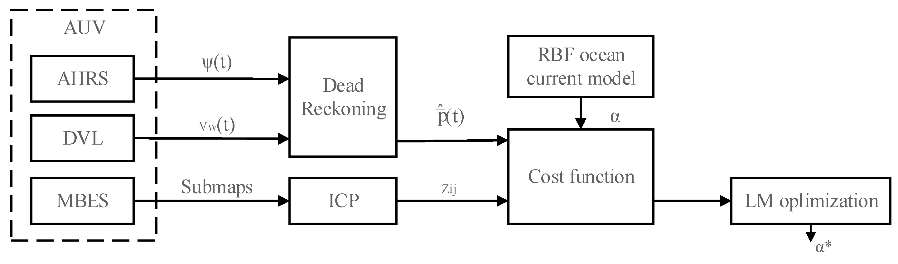
A diagram of the proposed ocean current estimation algorithm based on the RBF model is shown in Figure 5.

3. Results and Discussion

3.1. Simulation Setup

The pre-planned AUV trajectory is depicted in Figure 6, which is a lawn-mower trajectory widely adopted in ocean bathymetric missions. The AUV navigates along this pre-planned trajectory by employing dead-reckoning techniques for position estimation, using the water-track velocity measurement from DVL and the heading angles from the attitude and heading reference system (AHRS).

The motion of an AUV includes straight-line travel, turning, acceleration, and deceleration, with a maximum velocity of 3.0 m/s. The navigation duration is around 1.5 h. Figure 7 illustrates the dynamic process of the AUV throughout the simulation. To simulate realistic measurement errors in the DVL water-tracking mode, Gaussian velocity noise is introduced with distributions of $N(0 \mathrm{m}/\mathrm{s},{\left({\mathbf{v}}_{\mathrm{w}}\times 0.3\mathrm{\%} \mathrm{m}/\mathrm{s}\right)}^2)$ and $N(0 \mathrm{m}/\mathrm{s},{\left(0.003 \mathrm{m}/\mathrm{s}\right)}^2)$, where ${\mathbf{v}}_{\mathrm{w}}$ represents the water-relative velocity. These noise models account for velocity-dependent and constant-error components, respectively, ensuring a robust evaluation of the proposed method under realistic conditions.

We utilized bathymetric data derived from an open-access dataset supplied by the West Coast National Marine Sanctuaries Mapping project. This project was executed by the National Oceanic and Atmospheric Administration (NOAA) over a period spanning 8 May to 4 June 2017. The data were gathered using the Kongsberg EM302 multibeam echosounder, which was installed aboard the NOAA research vessel Nautilus. The resulting dataset provides a bathymetric point cloud with a spatial resolution of approximately 5 m. Figure 8 shows the bathymetric maps of two areas, Area 1 and Area 2, which are the operational regions for the AUV multibeam terrain surveys in Section 3.2 and Section 3.3, respectively.

3.2. Numerical Simulation and Results

In this section, the proposed RBF ocean current field estimation method is validated by numerical simulation. The first part is to obtain terrain-based relative position constraints when the AUV navigates in the simulated ocean current field. The second part is to solve the nonlinear optimization problem for RBF estimation using the relative position constraints.

3.2.1. Terrain-Based Relative Position Constraint Generation

To rigorously evaluate the robustness of the RBF method, we designed two distinct vortex flow models, illustrated by streamlines in Figure 9. In each subplot, the red dashed line represents the dead-reckoning trajectory of AUV, which is the estimated path based on the DVL water-tracking mode without accounting for ocean currents, abbreviated as DR-WT. The green solid line represents the true trajectory of AUV as it is influenced by the surrounding ocean current field, abbreviated as true. The origin of the coordinate system is set at the starting position of AUV. Case 1 describes a biased single vortex, representing an asymmetry flow field. Case 2 is a more complex flow field with two vortexes. The vortical flow field with double vortexes can be obtained by overlapping two opposite single flow fields. The parameters setting for each case are listed in

Table 1. Parameters of the vortical flow models used in numerical simulations.

Ocean Current Field	$\mathit{\omega }$	$\left({\mathit{c}}_{\mathit{x}},{\mathit{c}}_{\mathit{y}}\right)$	$\mathit{\sigma }$
Case 1	−600	(−2000, 1000)	5000
	−600	(2000, −1000)	5000
Case 2	400	(1000, −2000)	2500
	−400	(2000, −1000)	2500

, providing the vortex strength $\omega$, center coordinates $\left(c_x,c_y\right)$, and spatial scale parameter $\sigma$.

To establish terrain-based relative position constraints for the DR-WT path, we utilized multibeam bathymetric survey data collected during the mission in Area 1 of Figure 8. Figure 10a and Figure 11a illustrate the multibeam swaths corresponding to the true path for Case 1 and Case 2, respectively. Then, we applied an ICP algorithm proposed by Zhang et al. [33] and obtained a set of relative position constraints between the submaps. The total 43 terrain-based relative position constraints in Case 1 are shown in Figure 10b, with average errors of 0.7175 m in the x-direction and 0.9322 m in the y-direction. And, the total 39 terrain-based constraints in Case 2 are shown in Figure 11b, with the average errors of 0.6988 m in the x-direction and 0.9213 m in the y-direction.

3.2.2. Analysis of Ocean Current Estimation

To further validate the effectiveness of the proposed RBF-based ocean current field estimation method, we compare its performance against two commonly employed methods. For convenience, the two methods are called the constant current assumption (CCA) and the first-order polynomial current assumption (FOPCA). The CCA method [34] assumes that the ocean current velocity remains uniform and invariant across the entire simulation domain. The FOPCA method [35] models the ocean current velocity as a linear function of position, offering the capacity to capture spatial variations.

For the proposed RBF-based ocean current field estimation method, proper initialization of model parameters is crucial for the successful convergence of the Levenberg–Marquardt (LM) optimization algorithm. Appropriate initialization of the RBF model parameters is crucial before applying the LM optimization algorithm. Accordingly, five Gaussian RBFs are initialized with centers strategically placed to encompass the spatial domain of the AUV navigation region: four at the vertices of a bounding rectangle encompassing the DR-WT trajectory and one at the geometric center of the domain, represented as

$$\mathbf{c}\in \left\{\left(x_{\mathrm{m}\mathrm{i}\mathrm{n}},y_{\mathrm{m}\mathrm{i}\mathrm{n}}\right),\left(x_{\mathrm{m}\mathrm{i}\mathrm{n}},y_{\mathrm{m}\mathrm{a}\mathrm{x}}\right),\left(x_{\mathrm{m}\mathrm{a}\mathrm{x}},y_{\mathrm{m}\mathrm{i}\mathrm{n}}\right),\left(x_{\mathrm{m}\mathrm{a}\mathrm{x}},y_{\mathrm{m}\mathrm{a}\mathrm{x}}\right),\left({\displaystyle \frac{x_{\mathrm{m}\mathrm{i}\mathrm{n}}+x_{\mathrm{m}\mathrm{a}\mathrm{x}}}{2}},{\displaystyle \frac{y_{\mathrm{m}\mathrm{i}\mathrm{n}}+y_{\mathrm{m}\mathrm{a}\mathrm{x}}}{2}}\right)\right\}$$

(24)

For each RBF, the weight parameter $\omega$ is initialized as zero. And, the width parameter $\sigma$ is computed based on the spatial distribution of AUV trajectory points, as

$${\sigma }_i={\displaystyle \frac{2}{P}}\sum _{j=1}^P‖{\mathbf{p}}_j-{\mathbf{c}}_i‖$$

(25)

where $P$ denotes the number of AUV trajectory points, ${\mathbf{c}}_i$ is the center parameter of $i$-th RBF, and ${\sigma }_i$ is the width parameter of $i$-th RBF. This formulation assigns each basis function a width parameter that is twice the average distance between its center and all the trajectory points, ensuring appropriate spatial coverage.

All three methods will be evaluated using the simulated dataset described in the previous section, encompassing the two distinct vortex flow models (Cases 1 and 2). The ocean current estimation results based on CCA, FOPCA, and proposed RBF methods are shown in Figure 12 and Figure 13.

From the figures, it can be observed that the CCA method can only reflect the average trend of ocean current variations. It is limited in its ability to capture the finer details of the current variation. The FOPCA method is more capable of capturing the ocean current variations when compared to CCA. However, it still falls short in accurately estimating the dynamic changes in the ocean currents. The errors observed in the FOPCA results indicate that while the method can estimate the general ocean current behavior, it struggles with precise prediction, especially under complex flow conditions. The proposed RBF method demonstrates superior performance in accurately estimating the ocean current variations across two cases. As shown in Figure 11 and Figure 12, RBF provides a much closer alignment with the true ocean current, minimizing the absolute errors significantly. This indicates that the RBF method is highly effective in capturing both the general trends and the more intricate details of the ocean current changes, making it a promising approach for real-world oceanographic applications.

To quantitatively assess the performance of the ocean current estimation based on the proposed RBF model method, we introduce the root mean square error (RMSE) to evaluate the ocean current estimation result, which is defined as follows:

$$RMSE=\sqrt{{\displaystyle \frac{1}{P}}\sum _{i=1}^P{\left({\widehat{\mathit{v}}}_{\mathit{c}}\left(x_i,y_i\right)-{\mathit{v}}_{\mathit{c}}\left(x_i,y_i\right)\right)}^2}$$

(26)

where $\left(x_i,y_i\right)$ is the AUV position at time $t_i$, $P$ is the total number of waypoints along the AUV trajectory, $\left({\widehat{v}}_{c,x},{\widehat{v}}_{c,y}\right)$ is the estimated ocean current velocity using different ocean current model, and $\left(v_{c,x},v_{c,y}\right)$ is the true ocean current components encountered by the AUV.

Table 2. The ocean current estimation results under different methods in Case 1 and 2.

Ocean Current Field	Method	East Current RMSE (m/s)	North Current RMSE (m/s)
Case 1	CCA	0.0279	0.0343
	FOPCA	0.0020	0.0030
	Proposed RBF	0.0004	0.0002
Case 2	CCA	0.0125	0.0157
	FOPCA	0.0104	0.0133
	Proposed RBF	0.0005	0.0004

presents the east current RMSE and the north current RMSE for each case and for each method. Compared with CCA and FOPCA, the accuracy of current estimation result using the proposed RBF method shows significant improvement, with substantially lower RMSE values in both Case 1 and Case 2 for both the east and north current estimations.

3.2.3. Evaluation of Navigation Performance

After obtaining ocean current estimations along the AUV path, we evaluated four navigation methods: DR-WT, CCA, FOPCA and our proposed RBF method. The DR-WT method relies solely on DVL water-tracking measurements without accounting for ocean currents, while the other three methods incorporate ocean current estimates into their navigation solutions. This approach enables a direct comparison of their effectiveness in mitigating positional drift and enhancing accuracy relative to the baseline DR-WT method. Figure 14 and Figure 15 illustrate the navigation trajectories and corresponding positioning errors for all four methods across two case studies.

The quantitative assessment of positioning accuracy is presented in

Table 3. The statistic of positioning results in Case 1 and Case 2.

Ocean Current Field	Method	Positioning Error MAE (m)	Positioning Error RMSE (m)	Positioning Error Max (m)
Case 1	DR-WT	147.87	173.99	319.85
	CCA	40.11	44.24	64.21
	FOPCA	1.43	1.51	2.54
	Proposed RBF	0.48	0.54	0.95
Case 2	DR-WT	152.73	180.64	324.54
	CCA	12.31	14.30	26.64
	FOPCA	5.44	6.06	9.37
	Proposed RBF	0.81	0.85	1.17

, which compares the performance metrics of the four trajectory estimation methods across two distinct ocean current field cases. We employed three error metrics for evaluation, which are Mean Absolute Error (MAE), root mean square error (RMSE), and maximum error (Max), calculated as follows:

$$MAE={\displaystyle \frac{1}{P}}\sum _{i=1}^P‖\widehat{\mathbf{p}}\left(t_i\right)-\mathbf{p}\left(t_i\right)‖$$

(27)

$$RMSE=\sqrt{{\displaystyle \frac{1}{P}}\sum _{i=1}^P{‖\widehat{\mathbf{p}}\left(t_i\right)-\mathbf{p}\left(t_i\right)‖}^2}$$

(28)

$$MAX=\underset{i\in \left\{1,\dots ,P\right\}}{\max }‖\widehat{\mathbf{p}}\left(t_i\right)-\mathbf{p}\left(t_i\right)‖$$

(29)

where $\widehat{\mathbf{p}}\left(t_i\right)$ represents the estimated AUV position at time $t_i$, $\mathbf{p}\left(t_i\right)$ represents the ground true position, and $P$ is the number of position estimates.

3.2.4. Reconstruction of Ocean Current Field

In addition, we also reconstruct the ocean current field based on the optimized parameters. Figure 16a,c,e and Figure 17a,c,e show the reconstructed ocean current field based on CCA, FOPCA, and the proposed RBF method of Case 1 and 2, respectively. Figure 16b,d,f and Figure 17b,d,f show the norm of error $‖{\mathit{v}}_c-{\widehat{\mathit{v}}}_c‖$ in the field.

3.3. Experiment and Results Based on Real-World Oceanographic Data

To evaluate the feasibility and effectiveness of the proposed RBF-based ocean current field estimation method for AUV navigation, a simulated ocean current field was constructed using real-world oceanographic data. The dataset was sourced from the Hawaii Ocean Time-series (HOT) project, specifically collected during the HOT 312 cruise from 1 June to 4 June 2019 aboard the research vessel Kilo Moana. This vessel was equipped with a Teledyne RD Instruments Ocean Surveyor 38 kHz Acoustic Doppler Current Profiler (ADCP), configured to operate in both broadband mode (maximum range of 1200 m) and narrowband mode (maximum range of 1500 m), with an average measurement interval of approximately 5 min. The ADCP provided high-resolution current velocity profiles, enabling the reconstruction of a realistic ocean current field for simulation purposes.

We utilized horizontal current velocity data at depth of 756.4 m, as measured along trajectory of the vessel. Figure 18 shows the horizontal distribution of ocean current velocities at this depth as measured by ADCP onboard. Figure 19a presents the raw horizontal distribution of ocean current velocities at this depth, spanning an area of approximately 13.3 km by 14.9 km. To generate a continuous planar flow field suitable for AUV navigation simulations, the sparse ADCP measurements were interpolated using a triangle-based natural-neighbor interpolation method, as shown in Figure 19b. This interpolated field served as the ground truth for validating the RBF-based current estimation approach.

During the AUV navigation, a bathymetric survey was conducted to construct bathymetric submaps for terrain matching purposes in Area 2 of Figure 8. The multibeam swaths of AUV true path is shown in Figure 20. To acquire relative position measurements between these submaps, the dual-stage bathymetric ICP method proposed by Zhang et al. [33] was employed. This process resulted in the establishment of 41 terrain-based relative position constraints, as depicted in Figure 21. The average errors of these terrain-based relative position constraints were 0.7184 m in the x-direction and 0.9156 m in the y-direction.

Following the establishment of the constraints above, the proposed Levenberg–Marquardt optimization for RBF parameter estimation method was implemented for ocean current estimation. The initialization of RBF parameters was consistent with the settings described in Section 3.2. Meanwhile, CCA and FOPCA were also employed for comparison. Figure 22 presents the ocean current estimation results along the AUV path. As shown in Figure 22a,b, the proposed RBF method accurately captures the variations in both the east and north components of the ocean current, closely following the true current values. In contrast, the CCA method provides a constant approximation that fails to capture the variations, while the FOPCA method uses linear approximation with limited ability to represent the complex current patterns. The absolute estimation errors in the east and north directions for each method are illustrated in Figure 22c and Figure 22d, respectively. The proposed RBF demonstrates lower error magnitudes compared to both CCA and FOPCA. Quantitatively, the RMSE for the east component are 0.0074 m/s, 0.0058 m/s, and 0.0036 m/s for CCA, FOPCA, and the proposed RBF method, respectively. Similarly, for the north component, the RMSE are 0.0172 m/s, 0.0100 m/s, and the 0.0017 m/s, respectively. The results clearly demonstrate the superior accuracy of the proposed RBF method in estimating ocean currents.

To evaluate the impact of these ocean current results on navigation accuracy, Figure 23 provides a comparison of navigation trajectories and positioning errors for DR, CCA, FOPCA, and the proposed RBF approach. The trajectory comparison in Figure 23a shows that the RBF-based navigation path most closely follows the true trajectory, while the DR method exhibits the largest deviation. Figure 23b illustrates the positioning errors over time, with the proposed RBF method maintaining consistently lower errors throughout the navigation period. Quantitatively, the navigation accuracy is evaluated using MAE, RMSE, and maximum error. For the DR method, the MAE is 100.13 m, the RMSE is 114.80 m, and the maximum error reaches 192.94 m, indicating substantial drift due to uncompensated currents. The CCA method improves upon this, achieving an MAE of 25.30 m, an RMSE of 28.30 m, and a maximum error of 41.34 m, benefiting from its basic current approximation. The FOPCA method further reduces these values to an MAE of 17.96 m, an RMSE of 20.92 m, and a maximum error of 40.24 m, reflecting the advantage of its linear current model. However, the proposed RBF method outperforms all the others, with an MAE of just 3.13 m, an RMSE of 3.39 m, and a maximum error of 5.09 m. These metrics demonstrate that the RBF approach significantly enhances navigation precision by accurately capturing the dynamic nature of ocean currents.

The effectiveness of these methods in reconstructing the ocean current field is further explored in Figure 24, which compares the true current field with the reconstructed fields and their associated errors. Figure 24a presents the results for the CCA method, where the reconstructed ocean current field appears uniform and fails to capture the spatial variability of the true current. This limitation leads to significant errors across the domain, as evident in the error distribution in Figure 24b. Figure 24c,d depict the performance of the FOPCA method, showing a reconstructed field with linear gradients that can represent basic trends but struggles to replicate the intricate, nonlinear patterns of the true current. Consequently, the error field for FOPCA, while improved over CCA, still reveals noticeable discrepancies. In contrast, Figure 24e,f show the reconstruction of the proposed RBF method, which closely reflects the complex spatial variations in the true ocean current field. The resulting error field is minimally distributed, indicating a high degree of accuracy in capturing both the magnitude and direction of ocean currents. This superior reconstruction capability aligns with the low RMSE values of the RBF method for current estimation, reinforcing its effectiveness in modeling the dynamic and nonlinear characteristics of ocean currents.

4. Conclusions

This paper proposed an approach for ocean current field estimation in mid-water environments to enhance AUV navigation. A significant challenge in underwater navigation is the loss of DVL bottom-tracking when AUV operates beyond effective range from the seafloor, resulting in navigation drift due to unknown ocean currents.

The ocean current model is built upon the fundamental physical principle of incompressibility for ocean currents. By employing Gaussian RBFs as the stream potential function, the resulting velocity field is calculated as the gradient of stream function, inherently satisfying the mass conservation equation. This ensures a physical realistic and consistent representation of the current field. Our method uses MBES data to construct bathymetric submaps and the ICP algorithm as terrain-matching algorithm to obtain terrain-based relative position constraints among these submaps. These constraints are then integrated in to a nonlinear optimization problem, solved using the LM algorithm to determine the RBF parameter.

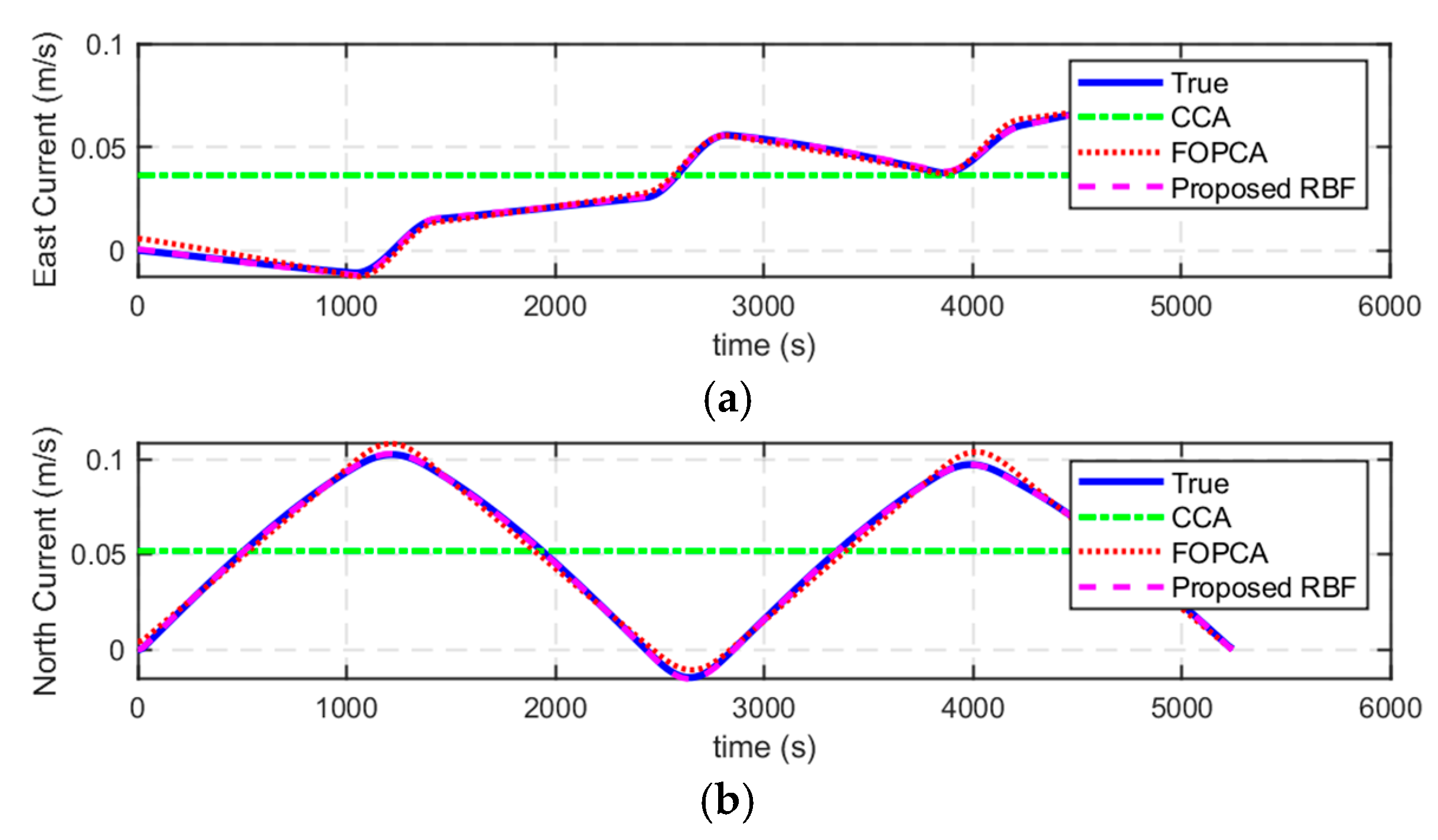
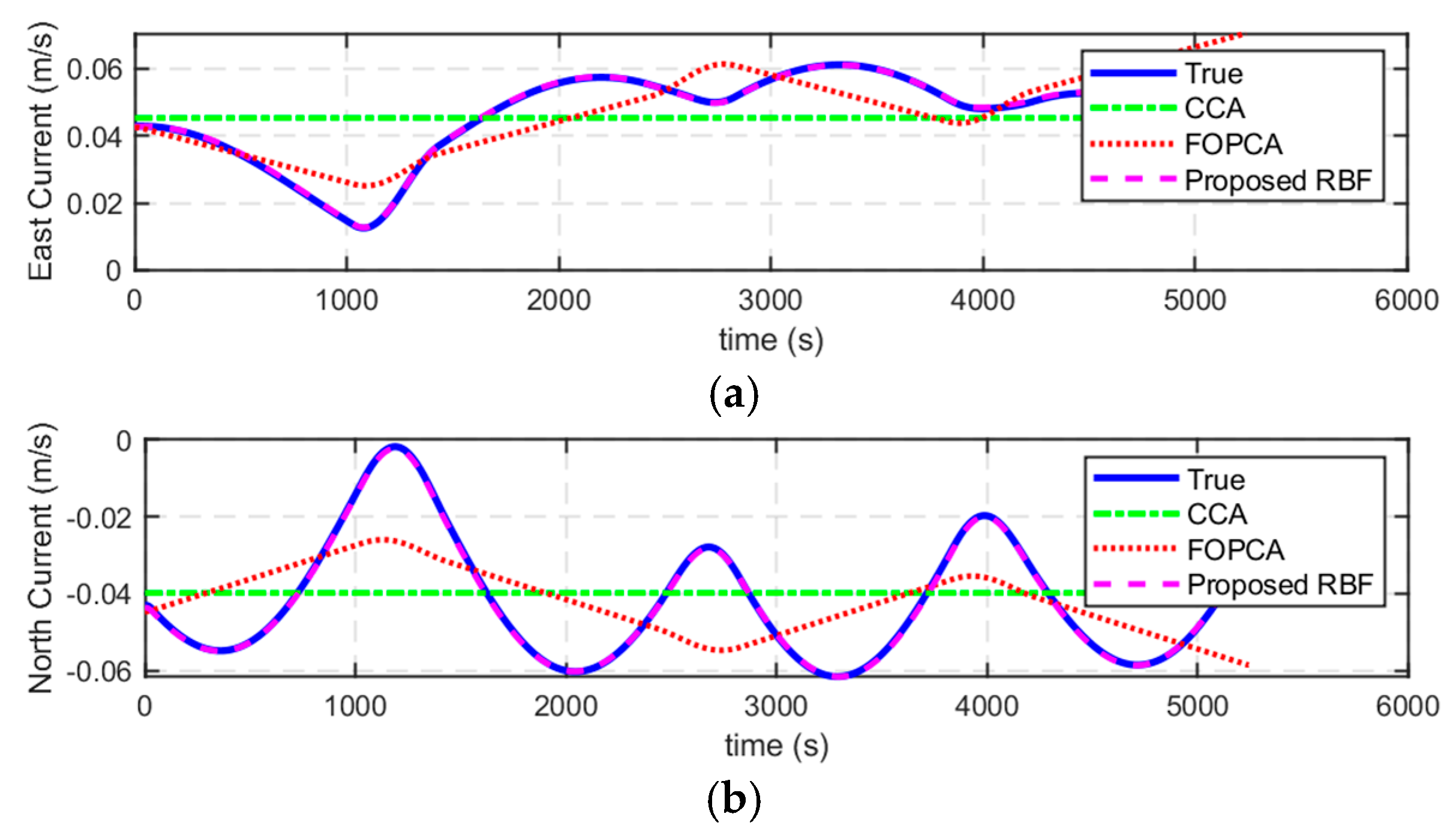
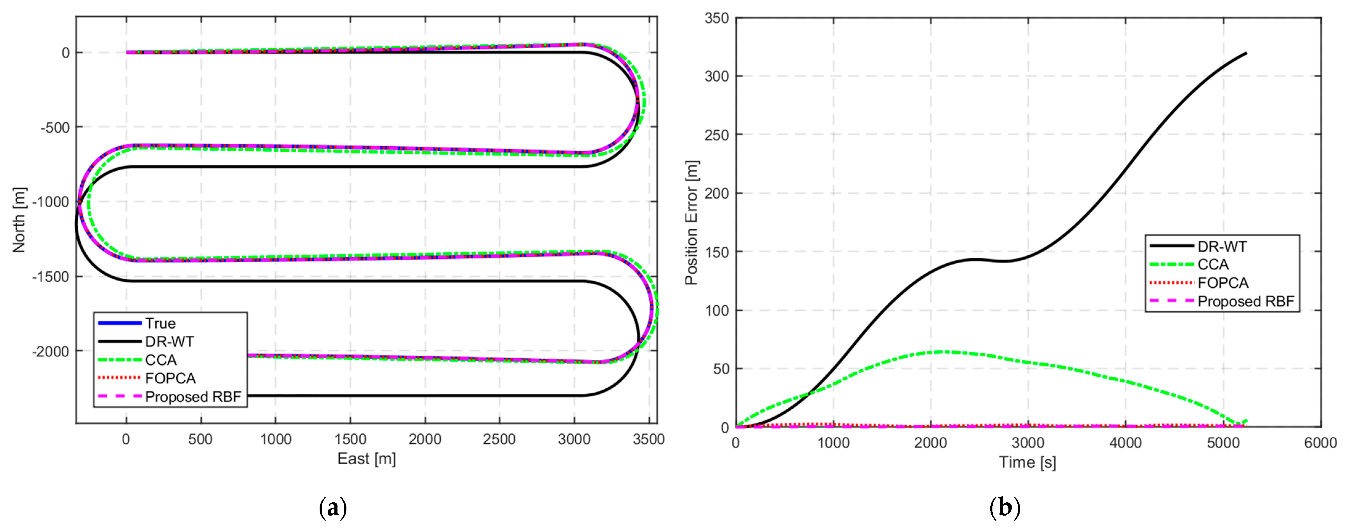
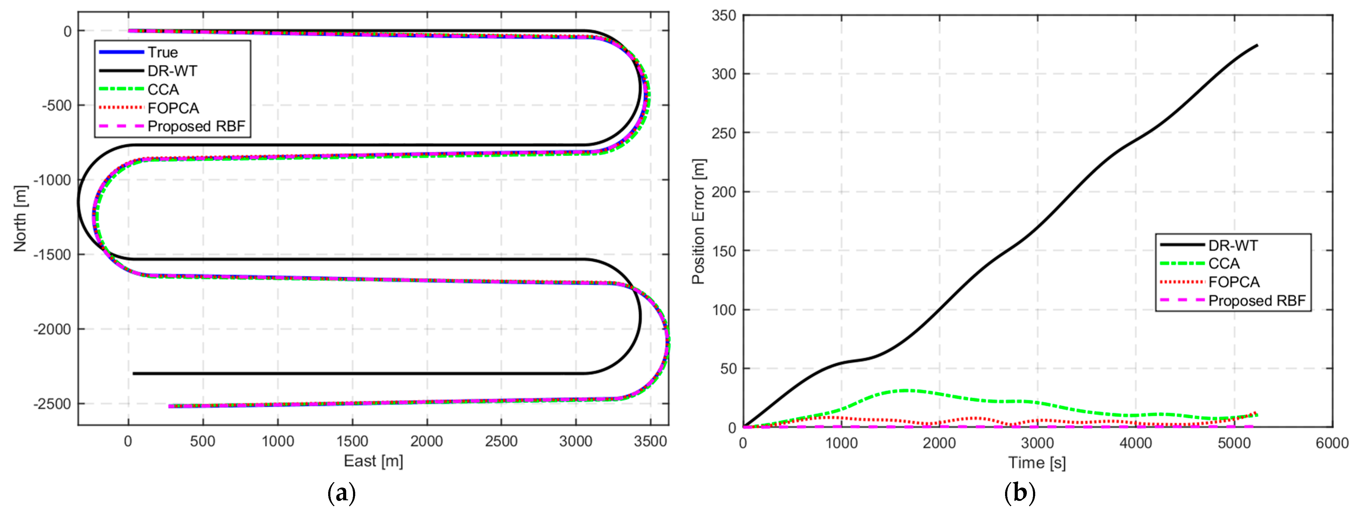
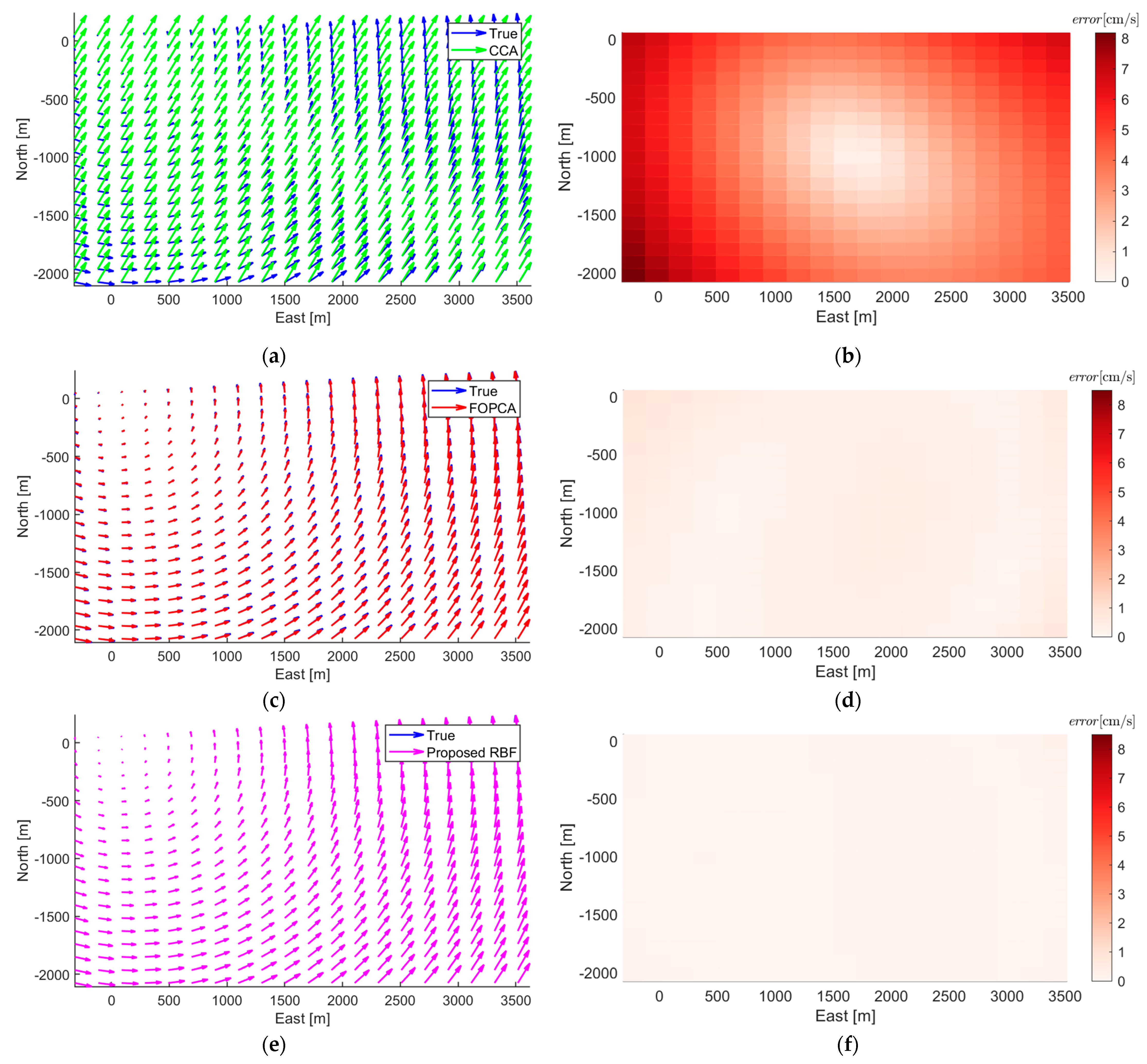
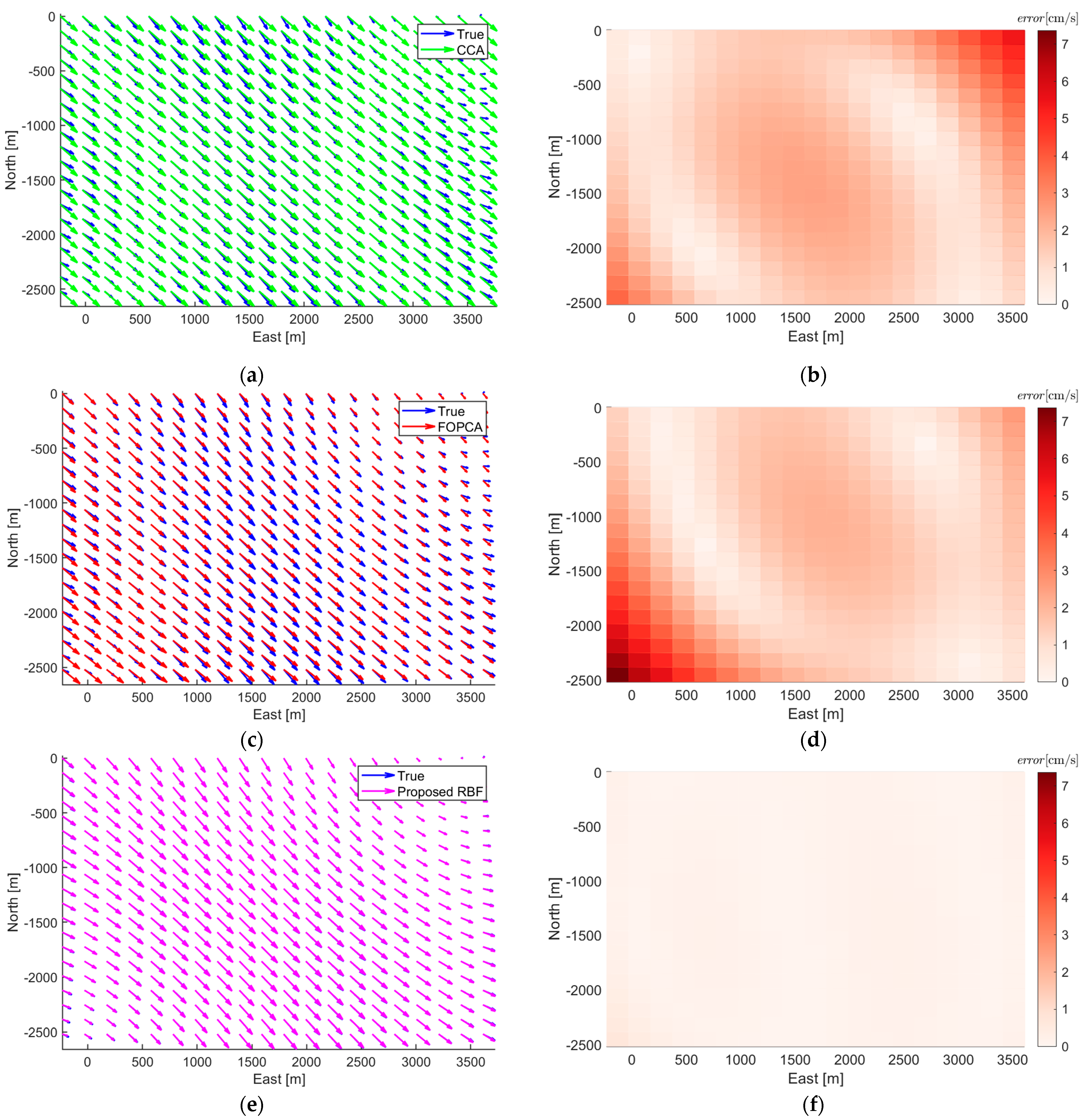
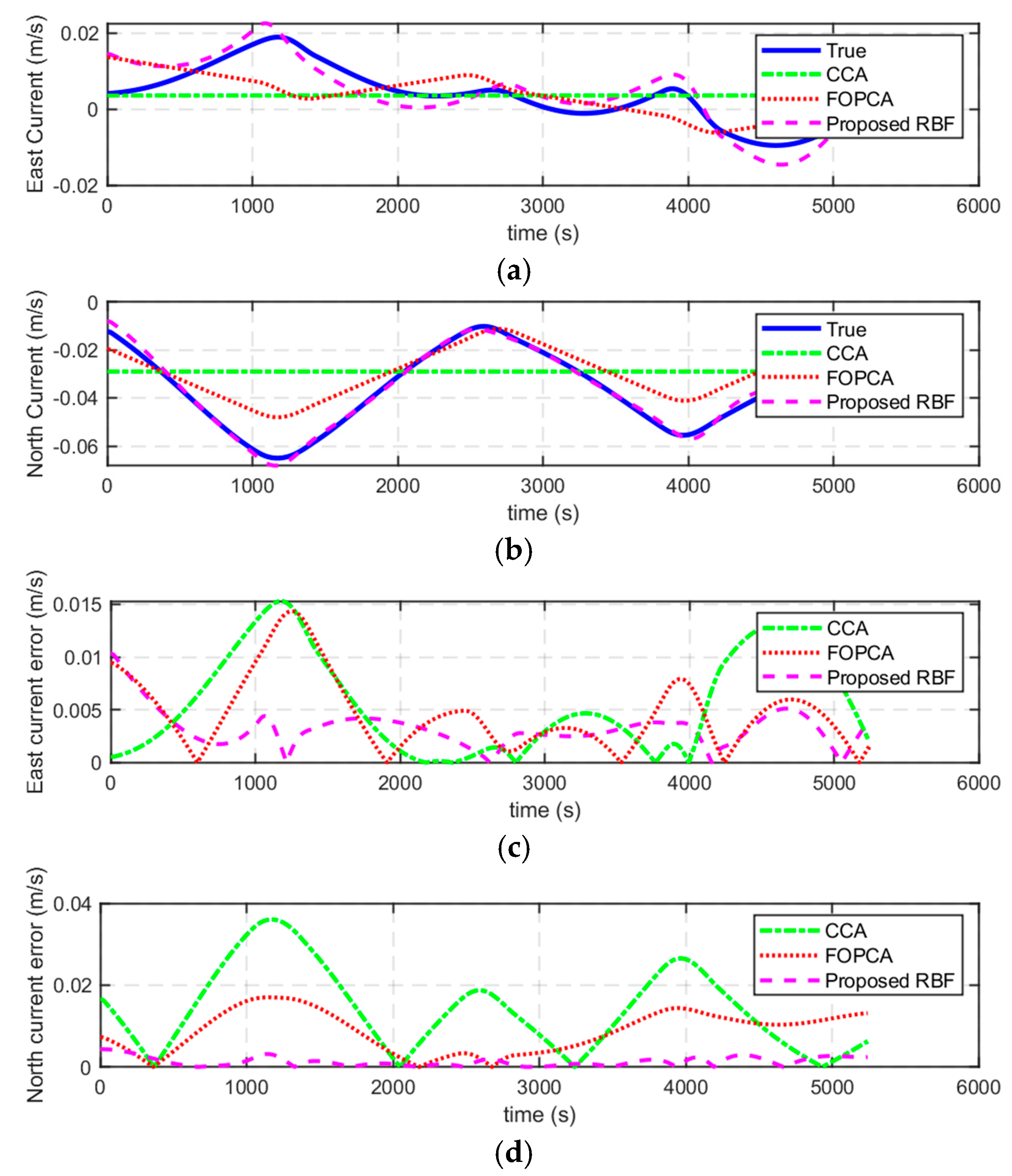
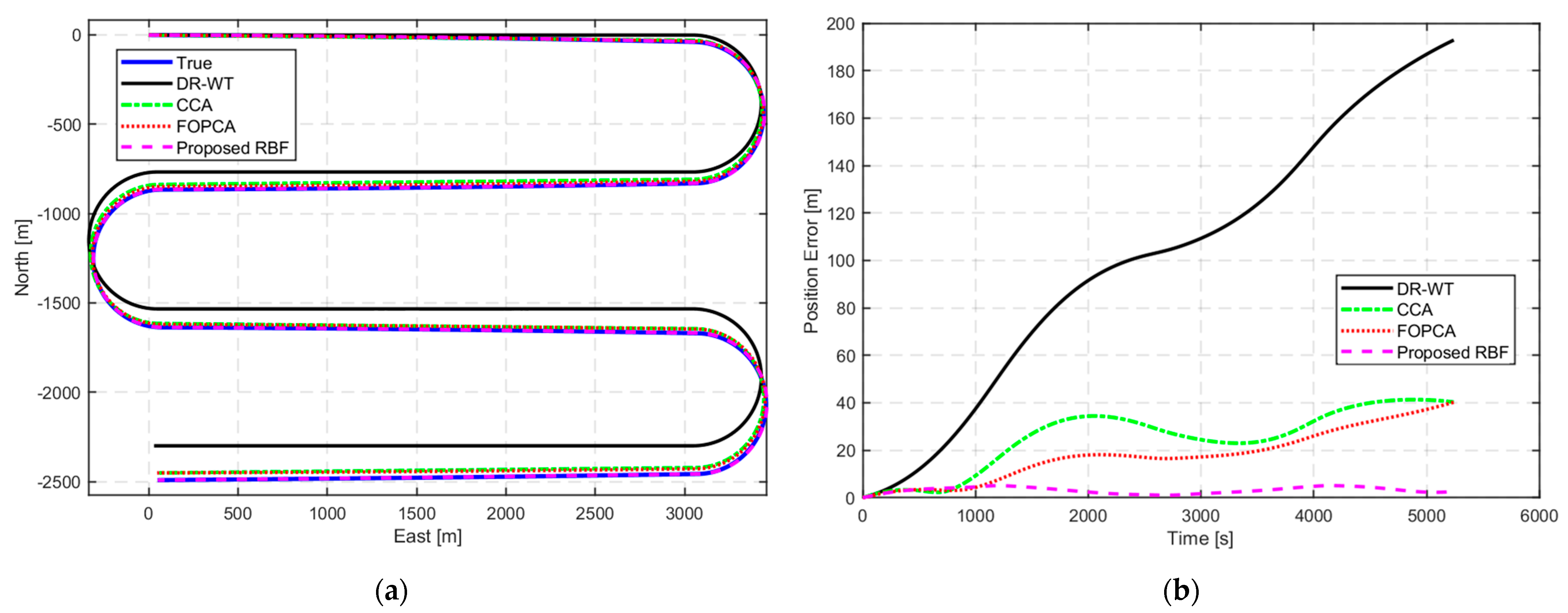
The numerical simulations and experiments validate the effectiveness of the proposed method, demonstrating high accuracy in ocean current estimation, substantial reductions in positioning errors, and significant improvements in ocean current field reconstruction. Compared with the ocean current estimation results based on simple constant current assumption and traditional first-order polynomial current assumption, the proposed RBF approach exhibits better performance in estimating ocean currents. In terms of navigation correction, the proposed RBF method substantially reduces positioning errors, showing the superiority in AUV localization during long-endurance missions in mid-water environments. Furthermore, the proposed RBF method excels in reconstructing the ocean current field, accurately capturing its complex spatial variations with minimal distributed errors.

However, the method has certain limitations that should be acknowledged. The accuracy of current field estimation depends on the quality and distribution of terrain-based relative position constraints, potentially limiting performance in regions with sparse bathymetric features. Additionally, the computational complexity increases with the number of RBF centers used to model the current field. In the future work, we will focus on developing adaptive RBF placement strategies and more efficient optimization techniques to address these limitations. We also aim to integrate complementary navigation technologies, such as acoustic positioning systems and geomagnetic measurements, to enhance robustness in diverse underwater environments.