
Enhancing Ocean Temperature and Salinity Reconstruction with Deep Learning: The Role of Surface Waves


Abstract
1. Introduction
2. Data and Methods
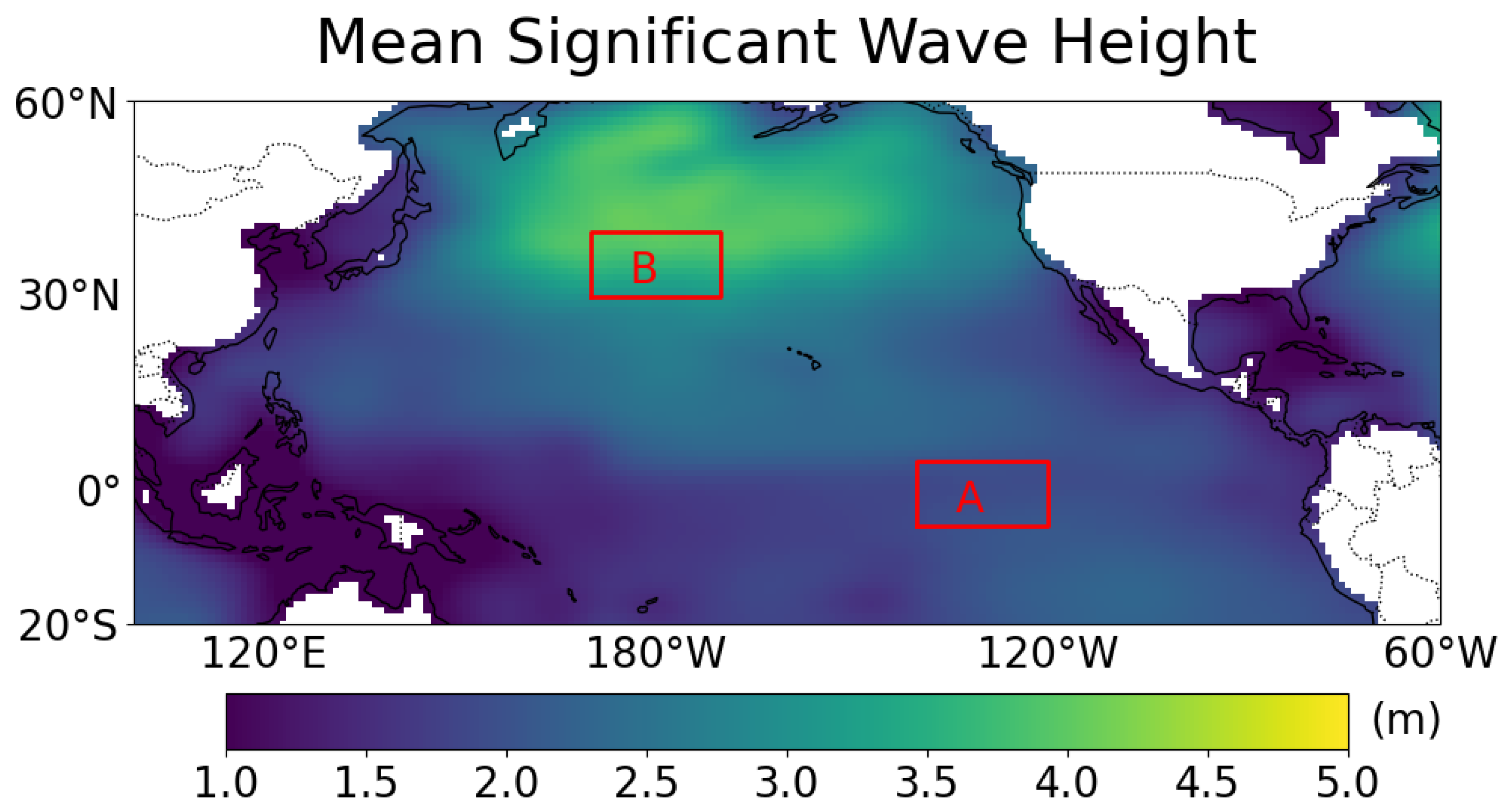
2.1. Study Regions
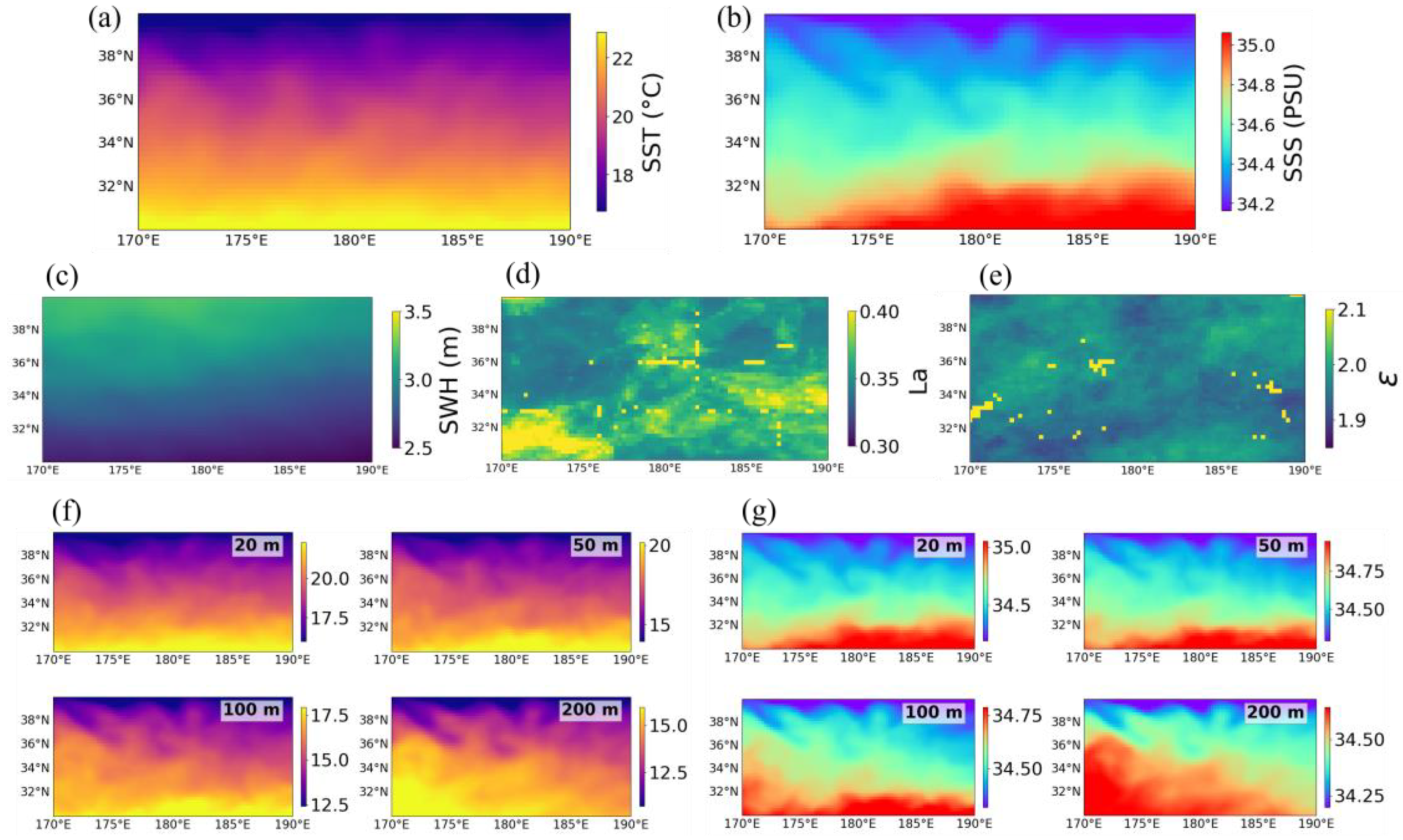
2.2. Data
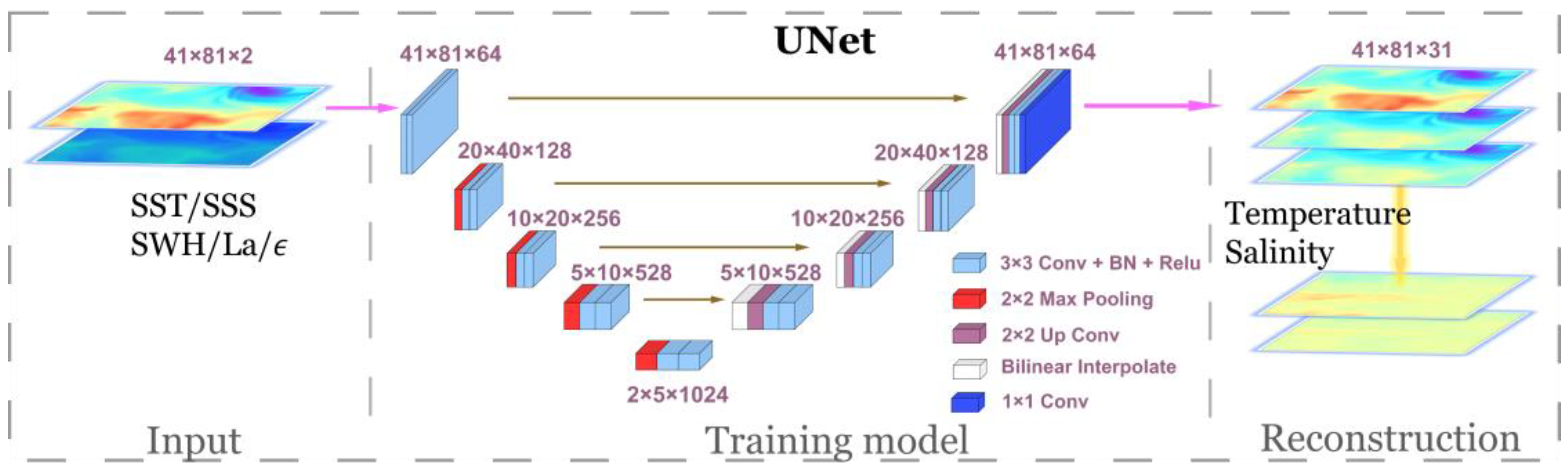
2.3. Methods
3. Results
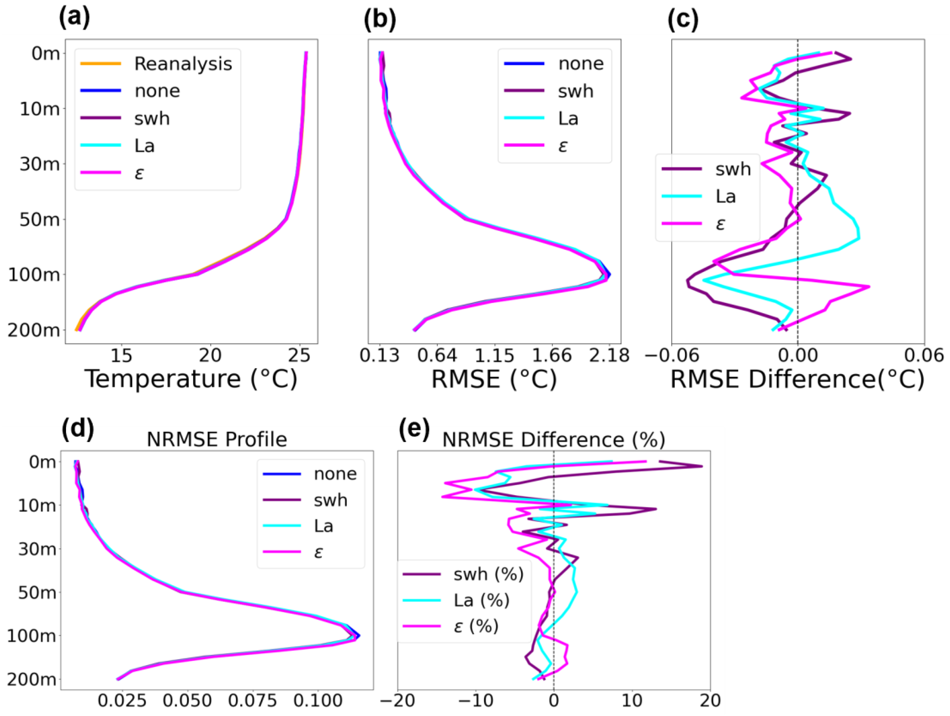
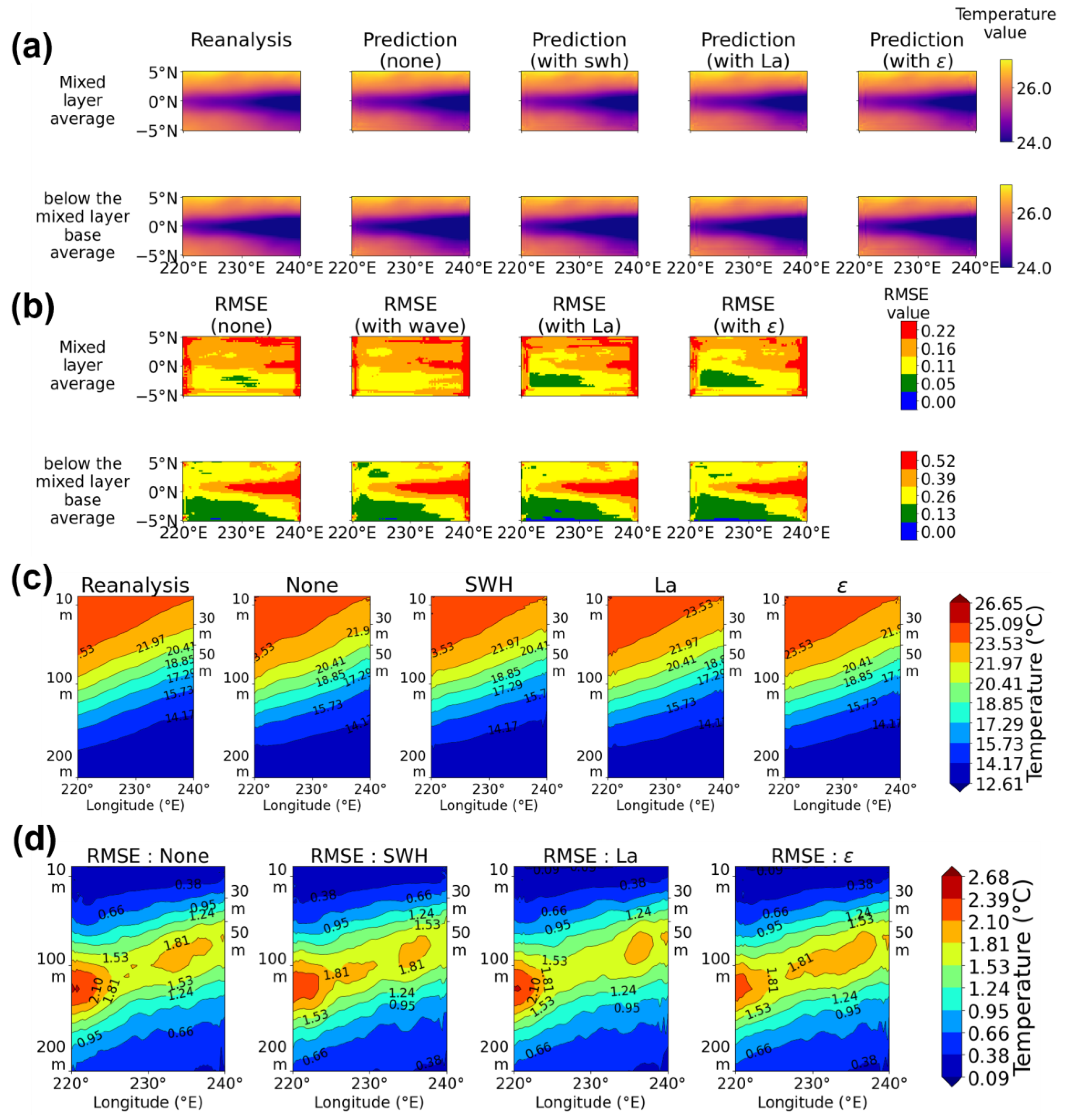
3.1. Temperature
3.1.1. Region A
3.1.2. Region B
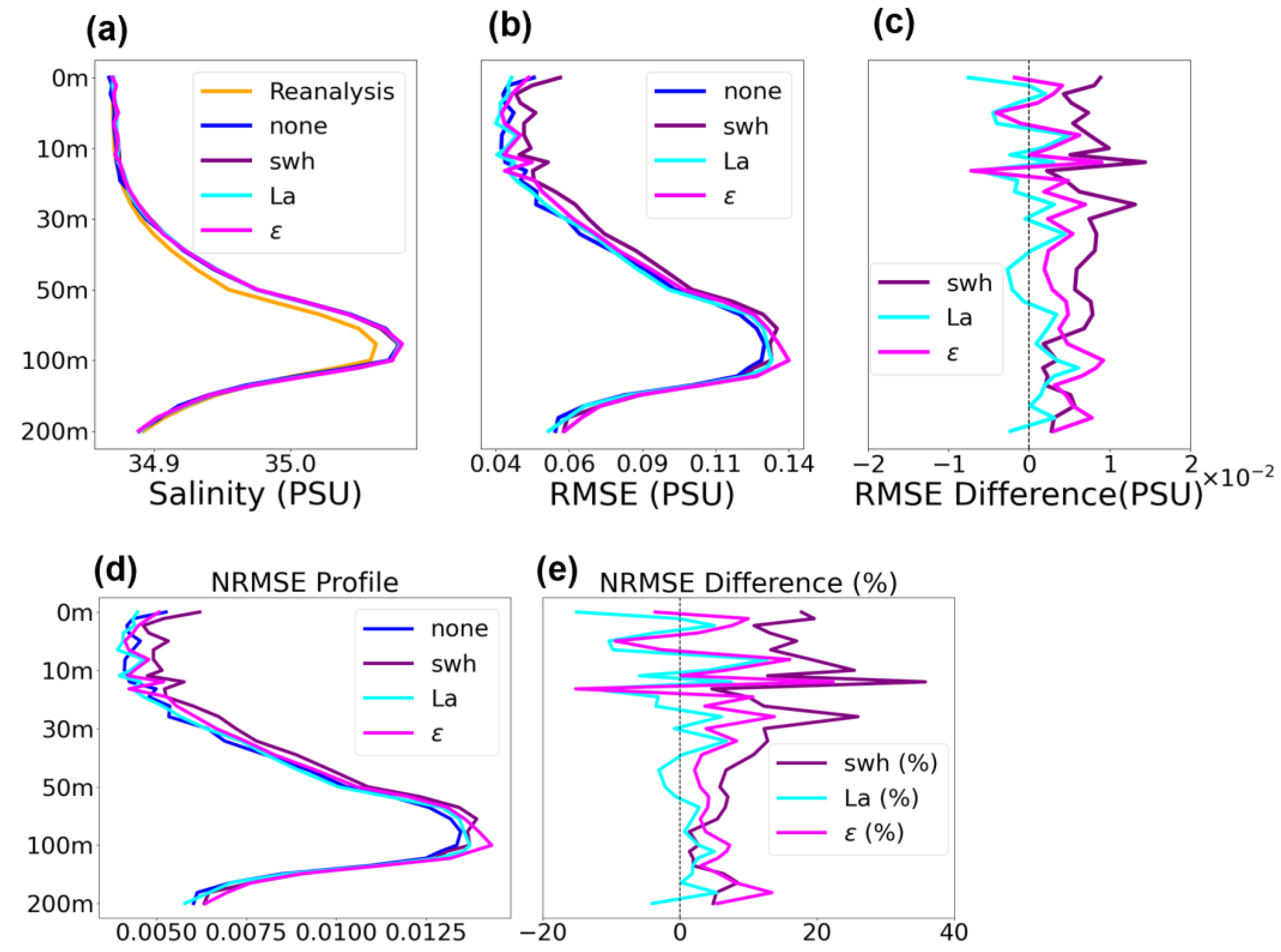
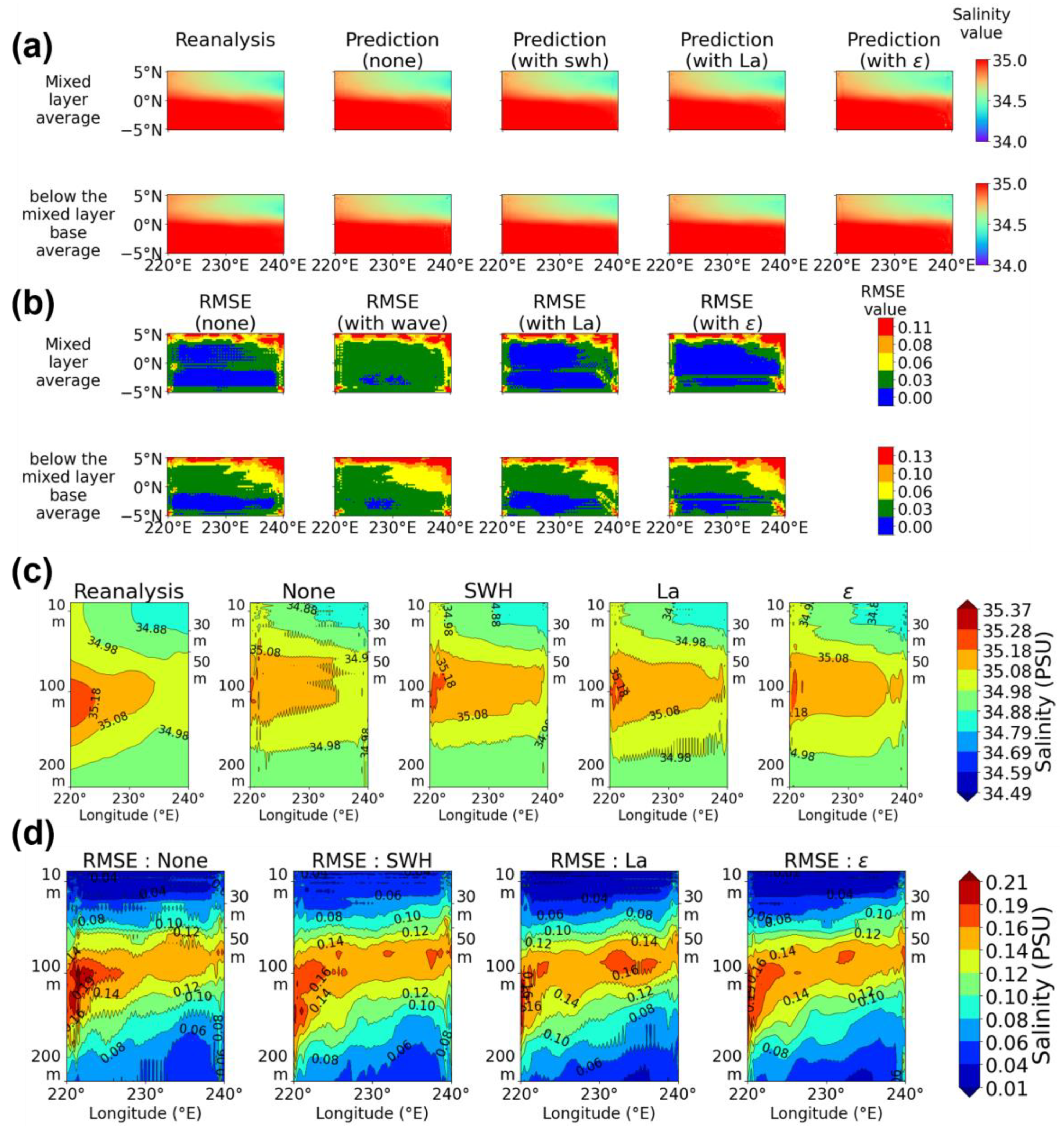
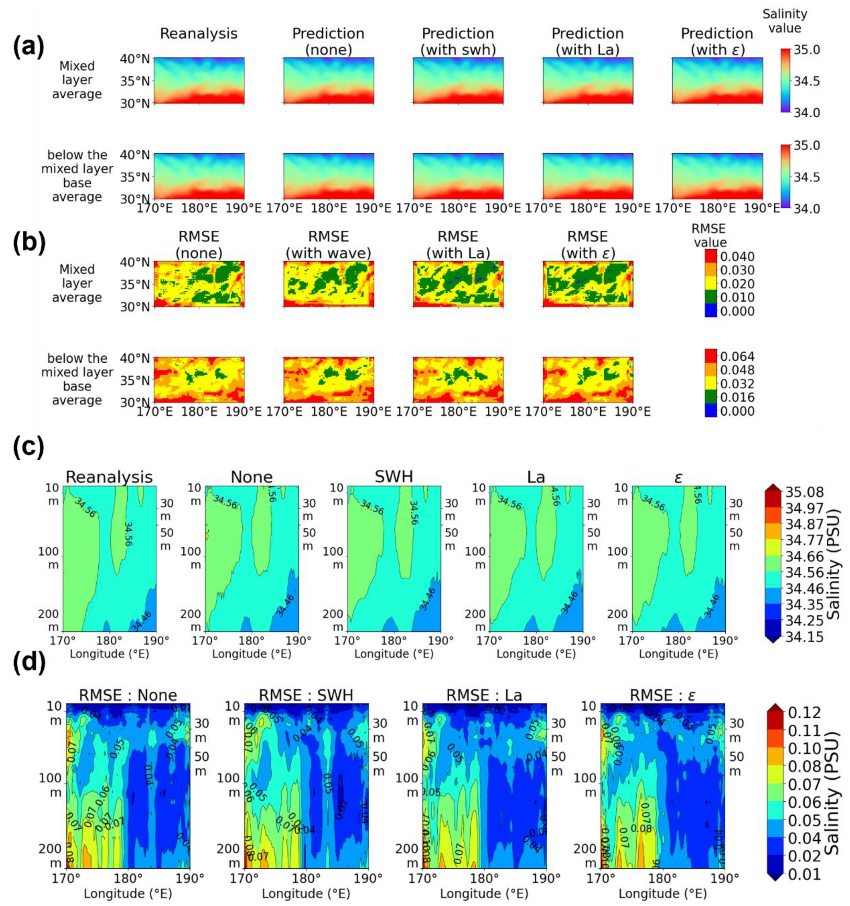
3.2. Salinity
3.2.1. Region A
3.2.2. Region B
3.3. Seasonality
4. Discussion
5. Conclusions
Author Contributions
Funding
Data Availability Statement
Acknowledgments
Conflicts of Interest
Abbreviations
| 3D | Three-dimensional |
| AMOC | Atlantic Meridional Overturning Circulation |
| EOF | Empirical Orthogonal Function |
| ROI | Reduced Optimal Interpolation |
| SST | Sea surface temperature |
| BPNN | Back-propagation neural network |
| FFNN | Feed-forward neural network |
| CNN | Convolutional Neural Network |
| SSHA | Sea surface height anomalies |
| La | Langmuir number |
| ε | Langmuir enhancement factor |
| ENSO | El Niño–Southern Oscillation |
| CMEMS | Copernicus Marine Environment Monitoring Service |
| GLOSEA | Global Ocean Reanalysis and Simulation Ensemble |
| SWH | Significant wave height |
| WAVERYS | CMEMS Global Wave Reanalysis product |
| SSS | Sea surface salinity |
| RMSE | Root Mean Square Error |
| NRMSE | Normalized Root Mean Square Error |
| R2 | Coefficient of determination |
| EUC | Equatorial undercurrent |
| SPTW | South Pacific Tropical Water |
| NECC | North Equatorial Countercurrent |
| SEC | South Equatorial Current |
| NPIW | North Pacific Intermediate Water |
References
- Moschos, E.; Barboni, A.; Stegner, A. Why Do Inverse Eddy Surface Temperature Anomalies Emerge? The Case of the Mediterranean Sea. Remote Sens. 2022, 14, 3807. [Google Scholar] [CrossRef]
- Sudre, F.; Dewitte, B.; Mazoyer, C.; Garçon, V.; Sudre, J.; Penven, P.; Rossi, V. Spatial and Seasonal Variability of Horizontal Temperature Fronts in the Mozambique Channel for Both Epipelagic and Mesopelagic Realms. Front. Mar. Sci. 2022, 9, 1045136. [Google Scholar] [CrossRef]
- Weijer, W.; Cheng, W.; Drijfhout, S.S.; Fedorov, A.V.; Hu, A.; Jackson, L.C.; Liu, W.; McDonagh, E.L.; Mecking, J.V.; Zhang, J. Stability of the Atlantic Meridional Overturning Circulation: A Review and Synthesis. J. Geophys. Res. Atmos. 2019, 124, 5336–5375. [Google Scholar] [CrossRef]
- Li Yi, D.; Wang, P. Global Wavenumber Spectra of Sea Surface Salinity in the Mesoscale Range Using Satellite Observations. Remote Sens. 2024, 16, 1753. [Google Scholar] [CrossRef]
- Buckley, M.W.; Marshall, J. Observations, inferences, and mechanisms of the Atlantic Meridional Overturning Circulation: A review. Rev. Geophys. 2016, 54, 5–63. [Google Scholar] [CrossRef]
- Dickey, T.; Lewis, M.; Chang, G. Optical Oceanography: Recent Advances and Future Directions Using Global Remote Sensing and In Situ Observations. Rev. Geophys. 2006, 44, RG000148. [Google Scholar] [CrossRef]
- Meng, L.; Yan, C.; Zhuang, W.; Zhang, W.; Yan, X.-H. Reconstruction of Three-Dimensional Temperature and Salinity Fields From Satellite Observations. J. Geophys. Res. Oceans 2021, 126, e2021JC017605. [Google Scholar] [CrossRef]
- Zhang, J.; Zhang, X.; Wang, X.; Ning, P.; Zhang, A. Reconstructing 3D Ocean Subsurface Salinity (OSS) from T–S Mapping via a Data-Driven Deep Learning Model. Ocean Model. 2023, 184, 102232. [Google Scholar] [CrossRef]
- Cassou, C.; Minvielle, M.; Terray, L.; Pérrigaud, C. A statistical–dynamical scheme for reconstructing ocean forcing in the Atlantic. Part I: Weather regimes as predictors for ocean surface variables. Clim. Dyn. 2011, 36, 19–39. [Google Scholar] [CrossRef]
- Lu, D.; Wang, C. Three-dimensional temperature field inversion calculation based on an artificial intelligence algorithm. Appl. Therm. Eng. 2023, 225, 120237. [Google Scholar] [CrossRef]
- Wong, M.S.; Jin, X.; Liu, Z.; Nichol, J.E.; Ye, S.; Jiang, P.; Chan, P.W. Geostationary Satellite Observation of Precipitable Water Vapor Using an Empirical Orthogonal Function (EOF) Based Reconstruction Technique over Eastern China. Remote Sens. 2015, 7, 5879–5900. [Google Scholar] [CrossRef]
- Kaplan, D.M.; Liu, A.M.C.; Abrams, M.T.; Warsofsky, I.S.; Kates, W.R.; White, C.D.; Kaufmann, W.E.; Reiss, A.L. Application of an automated parcellation method to the analysis of pediatric brain volumes. Psychiatry Res. Neuroimaging 1997, 76, 15–27. [Google Scholar] [CrossRef]
- Yuan, S.; Quiring, S.M. Comparison of three methods of interpolating soil moisture in Oklahoma. J. Climatol. 2017, 37, 987–997. [Google Scholar] [CrossRef]
- Merrifield, M.A.; Becker, J.M.; Ford, M.; Yao, Y. Observations and estimates of wave-driven water level extremes at the Marshall Islands. Geophys. Res. Lett. 2014, 41, 7245–7253. [Google Scholar] [CrossRef]
- Callaghan, F.M.; Grieve, S.M. Spatial resolution and velocity field improvement of 4D-flow MRI. Magn. Reson. Med. 2017, 78, 1959–1968. [Google Scholar] [CrossRef] [PubMed]
- Fujii, Y.; Kamachi, M. Three-dimensional analysis of temperature and salinity in the equatorial Pacific using a variational method with vertical coupled temperature–salinity empirical orthogonal function modes. J. Geophys. Res. Oceans, 2003; 108, 3297. [Google Scholar] [CrossRef]
- Burchard, H.; Craig, P.D.; Gemmrich, J.R.; van Haren, H.; Mathieu, P.-P.; Meier, H.E.M.; Nimmo Smith, W.A.M.; Prandke, H.; Rippeth, T.P.; Skyllingstad, E.D.; et al. Observational and numerical modeling methods for quantifying coastal ocean turbulence and mixing. Prog. Oceanogr. 2008, 76, 399–442. [Google Scholar] [CrossRef]
- Haidvogel, D.B.; Arango, H.; Budgell, W.P.; Cornuelle, B.D.; Curchitser, E.; Di Lorenzo, E.; Fennel, K.; Geyer, W.R.; Hermann, A.J.; Lanerolle, L.; et al. Ocean forecasting in terrain-following coordinates: Formulation and skill assessment of the Regional Ocean Modeling System. J. Comput. Phys. 2008, 227, 3595–3624. [Google Scholar] [CrossRef]
- Zhao, X.; Qi, J.; Yu, Y.; Zhou, L. Deep Learning for Ocean Temperature Forecasting: A Survey. Intell. Mar. Technol. Syst. 2024, 2, 28. [Google Scholar] [CrossRef]
- Cui, R.; Ma, L.; Hu, Y.; Wu, J.; Li, H. Research on High-Resolution Modeling of Satellite-Derived Marine Environmental Parameters Based on Adaptive Global Attention. Remote Sens. 2025, 17, 709. [Google Scholar] [CrossRef]
- Cheng, H.; Sun, L.; Li, J. Neural Network Approach to Retrieving Ocean Subsurface Temperatures from Surface Parameters Observed by Satellites. Water 2021, 13, 388. [Google Scholar] [CrossRef]
- Tian, T.; Cheng, L.; Wang, G.; Abraham, J.; Wei, W.; Ren, S.; Zhu, J.; Song, J.; Leng, H. Reconstructing Ocean Subsurface Salinity at High Resolution Using a Machine Learning Approach. Earth Syst. Sci. Data 2022, 14, 5037–5060. [Google Scholar] [CrossRef]
- Zhang, S.; Deng, Y.; Niu, Q.; Zhang, Z.; Che, Z.; Jia, S. Multivariate Temporal Self-Attention Network for Subsurface Thermohaline Structure Reconstruction. IEEE Trans. Geosci. Remote Sens. 2024, 61, 4507116. [Google Scholar] [CrossRef]
- Liu, Y.; Wang, H.; Jiang, F.; Zhou, Y.; Li, X. Reconstructing 3-D Thermohaline Structures for Mesoscale Eddies Using Satellite Observations and Deep Learning. IEEE Trans. Geosci. Remote Sens. 2024, 62, 4203916. [Google Scholar] [CrossRef]
- Wu, X.; Zhang, M.; Wang, Q.; Wang, X.; Chen, J.; Qin, Y. A Deep Learning Method for Inversing 3D Temperature Fields Using Sea Surface Data in Offshore China and the Northwest Pacific Ocean. J. Mar. Sci. Eng. 2024, 12, 2337. [Google Scholar] [CrossRef]
- Wei, M.; Shao, W.; Shen, W.; Hu, Y.; Zhang, Y.; Zuo, J. Contribution of Surface Waves to Sea Surface Temperatures in the Arctic Ocean. J. Ocean Univ. China 2024, 23, 1151–1162. [Google Scholar] [CrossRef]
- Ronneberger, O.; Fischer, P.; Brox, T. U-Net: Convolutional Networks for Biomedical Image Segmentation. arXiv 2015. [Google Scholar] [CrossRef]
- Chen, L.; Zhang, R.-H.; Gao, C. Effects of Temperature and Salinity on Surface Currents in the Equatorial Pacific. J. Geophys. Res. Oceans 2022, 127, e2021JC018175. [Google Scholar] [CrossRef]
- Belcher, S.E.; Grant, A.L.M.; Hanley, K.E.; Fox-Kemper, B.; Van Roekel, L.; Sullivan, P.P.; Large, W.G.; Brown, A.; Hines, A.; Calvert, D.; et al. A global perspective on Langmuir turbulence in the ocean surface boundary layer. Geophys. Res. Lett. 2012, 39, L052932. [Google Scholar] [CrossRef]
- Wang, P.; Özgökmen, T.M. Langmuir circulation with explicit surface waves from moving-mesh modeling. Geophys. Res. Lett. 2018, 45, 216–226. [Google Scholar] [CrossRef]
- McWilliams, J.C.; Sullivan, P.P.; Moeng, C.-H. Langmuir turbulence in the ocean. J. Fluid Mech. 1997, 334, 1–30. [Google Scholar] [CrossRef]
- McWilliams, J.C.; Huckle, E.; Liang, J.; Sullivan, P.P. Langmuir Turbulence in Swell. J. Phys. Oceanogr. 2014, 44, 870–890. [Google Scholar] [CrossRef]
- Van Roekel, L.; Fox-Kemper, B.; Sullivan, P.; Hamlington, P.; Haney, S. The Form and Orientation of Langmuir Cells for Misaligned Winds and Waves. J. Geophys. Res. Oceans. 2012, 117(C5), C05001. [Google Scholar] [CrossRef]
- Wang, P.; McWilliams, J.C.; Yuan, J.; Liang, J.-H. Langmuir mixing schemes based on a modified K-Profile Parameterization. J. Adv. Model. Earth Syst. 2025, 17, e2024MS004729. [Google Scholar] [CrossRef]
- McWilliams, J.C.; Sullivan, P.P. Vertical Mixing by Langmuir Circulations. Spill Sci. Technol. Bull. 2000, 6, 225–237. [Google Scholar] [CrossRef]
- Niedzielski, T. El Niño/Southern Oscillation and Selected Environmental Consequences. Adv. Geophys. 2014, 55, 77–122. [Google Scholar] [CrossRef]
- Ueno, H.; Bracco, A.; Barth, J.A.; Budyansky, M.V.; Hasegawa, D.; Itoh, S.; Kim, S.Y.; Ladd, C.; Lin, X.; Park, Y.-G.; et al. Review of oceanic mesoscale processes in the North Pacific: Physical and biogeochemical impacts. Prog. Oceanogr. 2023, 212, 102955. [Google Scholar] [CrossRef]
- Le Traon, P.Y.; Reppucci, A.; Fanjul, E.A.; Aouf, L.; Behrens, A.; Belmonte, M.; Bentamy, A.; Bertino, L.; Brando, V.E.; Kreiner, M.B.; et al. From Observation to Information and Users: The Copernicus Marine Service Perspective. Front. Mar. Sci. 2019, 6, 234. [Google Scholar] [CrossRef]
- Legg, S.; McWilliams, J.; Gao, J. Localization of Deep Ocean Convection by a Mesoscale Eddy. J. Phys. Oceanogr. 1998, 28, 944–970. [Google Scholar] [CrossRef]
- Wang, C.; Fiedler, P.C. ENSO variability and the eastern tropical Pacific: A review. Prog. Oceanogr. 2006, 69, 239–266. [Google Scholar] [CrossRef]
- Amador, J.A.; Alfaro, E.J.; Lizano, O.G.; Magaña, V.O. Atmospheric forcing of the eastern tropical Pacific: A review. Prog. Oceanogr. 2006, 69, 101–142. [Google Scholar] [CrossRef]
- Li, Q.; Reichl, B.G.; Fox-Kemper, B.; Adcroft, A.J.; Belcher, S.E.; Danabasoglu, G.; Grant, A.L.M.; Griffies, S.M.; Hallberg, R.; Hara, T.; et al. Comparing Ocean Surface Boundary Vertical Mixing Schemes Including Langmuir Turbulence. J. Adv. Model. Earth Syst. 2019, 11, 3545–3592. [Google Scholar] [CrossRef]
- Li, Q.; Webb, A.; Fox-Kemper, B.; Craig, A.; Danabasoglu, G.; Large, W.G.; Vertenstein, M. Langmuir mixing effects on global climate: WAVEWATCH III in CESM. Ocean Model. 2016, 103, 145–160. [Google Scholar] [CrossRef]
- Tsuchiya, M.; Lukas, R.; Fine, R.A.; Firing, E.; Lindstrom, E. Source waters of the Pacific Equatorial Undercurrent. Prog. Oceanogr. 1989, 23, 101–147. [Google Scholar] [CrossRef]
- Kuntz, L.B.; Schrag, D.P. Subtropical modulation of the equatorial undercurrent: A mechanism of Pacific variability. Clim. Dyn. 2021, 56, 1937–1949. [Google Scholar] [CrossRef]
- Wang, P.; McWilliams, J.C.; Wang, D.; Li Yi, D. Conservative Surface Wave Effects on a Wind-Driven Coastal Upwelling System. J. Phys. Oceanogr. 2022, 53, 37–55. [Google Scholar] [CrossRef]
- Xuan, A.; Deng, B.-Q.; Shen, L. Study of wave effect on vorticity in Langmuir turbulence using wave-phase-resolved large-eddy simulation. J. Fluid Mech. 2019, 875, 173–224. [Google Scholar] [CrossRef]
- Huang, R.X. Mixing and Energetics of the Oceanic Thermohaline Circulation. J. Phys. Oceanogr. 1999, 29, 727–746. [Google Scholar] [CrossRef]
- Sun, W.; An, M.; Liu, J.; Liu, J.; Yang, J.; Tan, W.; Dong, C.; Liu, Y. Comparative analysis of four types of mesoscale eddies in the Kuroshio-Oyashio extension region. Front. Mar. Sci. 2022, 9, 984244. [Google Scholar] [CrossRef]
- Xiao, B.; Qiao, F.; Shu, Q.; Yin, X.; Wang, G.; Wang, S. Development and validation of a global 1/32° surface-wave–tide–circulation coupled ocean model: FIO-COM32. Geosci. Model Dev. 2023, 16, 1755–1778. [Google Scholar] [CrossRef]
- Zhou, J.; Zhou, G.; Liu, H.; Li, Z.; Cheng, X. Mesoscale Eddy-Induced Ocean Dynamic and Thermodynamic Anomalies in the North Pacific. Front. Mar. Sci. 2021, 8, 756918. [Google Scholar] [CrossRef]
- Nakano, H.; Tsujino, H.; Sakamoto, K.; Urakawa, S.; Toyoda, T.; Yamanaka, G. Identification of the fronts from the Kuroshio Extension to the Subarctic Current using absolute dynamic topographies in satellite altimetry products. J. Oceanogr. 2018, 74, 393–420. [Google Scholar] [CrossRef]
- Dalton, F.N.; Maggio, A.; Piccinni, G. Effect of root temperature on plant response functions for tomato: Comparison of static and dynamic salinity stress indices. Plant Soil 1997, 192, 307–319. [Google Scholar] [CrossRef]
- Malan, N.; Durgadoo, J.V.; Biastoch, A.; Reason, C.; Hermes, J. Multidecadal Wind Variability Drives Temperature Shifts on the Agulhas Bank. J. Geophys. Res. Oceans 2019, 124, 3021–3035. [Google Scholar] [CrossRef]
- Sumner, D.M.; Belaineh, G. Evaporation, Precipitation, and Associated Salinity Changes at a Humid, Subtropical Estuary. Estuaries 2005, 28, 844–855. [Google Scholar] [CrossRef]
- Gregg, M.C.; Cox, C.S. The vertical microstructure of temperature and salinity. Deep Sea Res. Oceanogr. Abstr. 1972, 19, 355–376. [Google Scholar] [CrossRef]
- Liang, C.-R.; Shang, X.-D.; Qi, Y.-F.; Chen, G.-Y.; Yu, L.-H. Enhanced Diapycnal Mixing Between Water Masses in the Western Equatorial Pacific. J. Geophys. Res. Oceans 2019, 124, 8102–8115. [Google Scholar] [CrossRef]
- Moum, J.N.; Natarov, A.; Richards, K.J.; Shroyer, E.L.; Smyth, W.D. Mixing in equatorial oceans. In Ocean Mixing: Drivers, Mechanisms and Impacts; Elsevier: Amsterdam, The Netherlands, 2022; pp. 257–273. [Google Scholar] [CrossRef]
- Guadayol, Ò.; Peters, F.; Marrasé, C.; Gasol, J.M.; Roldán, C.; Berdalet, E.; Massana, R.; Sabata, A. Episodic meteorological and nutrient-load events as drivers of coastal planktonic ecosystem dynamics: A time-series analysis. Mar. Ecol. Prog. Ser. 2009, 381, 139–155. [Google Scholar] [CrossRef]
- Kolodziejczyk, N.; Marin, F.; Bourlés, B.; Gouriou, Y.; Berger, H. Seasonal variability of the equatorial undercurrent termination and associated salinity maximum in the Gulf of Guinea. Clim. Dyn. 2014, 43, 3025–3046. [Google Scholar] [CrossRef]
- Brainerd, K.E.; Gregg, M.C. Surface mixed and mixing layer depths. Deep Sea Res. Part I 1995, 42, 1521–1543. [Google Scholar] [CrossRef]
- McGee, D.; Moreno-Chamarro, E.; Green, B.; Marshall, J.; Galbraith, E.; Bradtmiller, L. Hemispherically asymmetric trade wind changes as signatures of past ITCZ shifts. Quat. Sci. Rev. 2018, 180, 214–228. [Google Scholar] [CrossRef]
- Camberlin, P.; Janicot, S.; Poccard, I. Seasonality and atmospheric dynamics of the teleconnection between African rainfall and tropical sea-surface temperature: Atlantic vs. ENSO. Int. J. Climatol. 2001, 21, 973–1005. [Google Scholar] [CrossRef]
- Li, B.; Yuan, D.; Zhou, H. Water masses in the far western equatorial Pacific during the winters of 2010 and 2012. J. Oceanol. Limnol. 2018, 36, 1459–1474. [Google Scholar] [CrossRef]
- Li, Z.; Fedorov, A.V. Coupled dynamics of the North Equatorial Countercurrent and Intertropical Convergence Zone with relevance to the double-ITCZ problem. Proc. Natl. Acad. Sci. USA 2022, 119, e2120309119. [Google Scholar] [CrossRef] [PubMed]
- Toole, J.M.; Zou, E.; Millard, R.C. On the circulation of the upper waters in the western equatorial Pacific Ocean. Deep Sea Res. Part A 1988, 35, 1451–1482. [Google Scholar] [CrossRef]
- Hatayama, T. Transformation of the Indonesian Throughflow Water by Vertical Mixing and Its Relation to Tidally Generated Internal Waves. J. Oceanogr. 2004, 60, 569–585. [Google Scholar] [CrossRef]
- Nakano, T.; Kaneko, I.; Endoh, M.; Kamachi, M. Interannual and Decadal Variabilities of NPIW Salinity Minimum Core Observed along JMA’s Hydrographic Repeat Sections. J. Oceanogr. 2005, 61, 681–697. [Google Scholar] [CrossRef]
- Yasuda, I. The origin of the North Pacific Intermediate Water. J. Geophys. Res. Oceans 1997, 102, 893–909. [Google Scholar] [CrossRef]
- Nagano, A.; Uehara, K.; Suga, T.; Kawai, Y.; Ichikawa, H.; Cronin, M.F. Origin of near-surface high-salinity water observed in the Kuroshio Extension region. J. Oceanogr. 2014, 70, 389–403. [Google Scholar] [CrossRef]
- Liao, G.-H.; Hu, X.-K.; Xu, S.-M.; Wu, K.-M.; Dong, J.-H.; Dong, C.-M. Impact of symmetric instability parametrization scheme on the upper ocean layer in a high-resolution global ocean model. Deep Sea Res. Part II 2022, 202, 105147. [Google Scholar] [CrossRef]
- Kobashi, F.; Kubokawa, A. New developments in mode-water research: Dynamic and climatic effects. Review on North Pacific Subtropical Countercurrents and Subtropical Fronts: Role of mode waters in ocean circulation and climate. J. Oceanogr. 2012, 68, 21–43. [Google Scholar] [CrossRef]
- Miller, A.J.; Schneider, N. Interdecadal climate regime dynamics in the North Pacific Ocean: Theories, observations and ecosystem impacts. Prog. Oceanogr. 2000, 47, 355–379. [Google Scholar] [CrossRef]
- Luo, S.; Jing, Z.; Qi, Y. Submesoscale Flows Associated with Convergent Strain in an Anticyclonic Eddy of the Kuroshio Extension: A High-resolution Numerical Study. Ocean Sci. J. 2020, 55, 249–264. [Google Scholar] [CrossRef]
- Li, X.; Zhou, G.; Cheng, X. Decadal-Scale Influence of the Kuroshio and Oyashio Extension Fronts on Atmospheric Circulation and Storm Track. J. Geophys. Res. Atmos. 2024, 129, e2023JD039589. [Google Scholar] [CrossRef]
- Wu, R.; Kirtman, B.P. Roles of Indian and Pacific Ocean air–sea coupling in tropical atmospheric variability. Clim. Dyn. 2005, 25, 155–170. [Google Scholar] [CrossRef]
- Coumou, D.; Di Capua, G.; Vavrus, S.; Wang, L.; Wang, S. The influence of Arctic amplification on mid-latitude summer circulation. Nat. Commun. 2018, 9, 2959. [Google Scholar] [CrossRef]
- Qiao, F.; Yuan, Y.; Yang, Y.; Zheng, Q.; Xia, C.; Ma, J. Wave-induced mixing in the upper ocean: Distribution and application to a global ocean circulation model. Geophys. Res. Lett. 2004, 31, L1960–L1965. [Google Scholar] [CrossRef]


| Experiment Name | Inputs | Outputs |
|---|---|---|
| Exp1: Baseline (none wave) | SST | 3D Temperature |
| Exp2: swh | SST, SWH | |
| Exp3: La | SST, La | |
| Exp4: ε | SST, ε |
Disclaimer/Publisher’s Note: The statements, opinions and data contained in all publications are solely those of the individual author(s) and contributor(s) and not of MDPI and/or the editor(s). MDPI and/or the editor(s) disclaim responsibility for any injury to people or property resulting from any ideas, methods, instructions or products referred to in the content. |
© 2025 by the authors. Licensee MDPI, Basel, Switzerland. This article is an open access article distributed under the terms and conditions of the Creative Commons Attribution (CC BY) license (https://creativecommons.org/licenses/by/4.0/).
Share and Cite
Yu, X.; Yi, D.L.; Wang, P. Enhancing Ocean Temperature and Salinity Reconstruction with Deep Learning: The Role of Surface Waves. J. Mar. Sci. Eng. 2025, 13, 910. https://doi.org/10.3390/jmse13050910
Yu X, Yi DL, Wang P. Enhancing Ocean Temperature and Salinity Reconstruction with Deep Learning: The Role of Surface Waves. Journal of Marine Science and Engineering. 2025; 13(5):910. https://doi.org/10.3390/jmse13050910
Chicago/Turabian StyleYu, Xiaoyu, Daling Li Yi, and Peng Wang. 2025. "Enhancing Ocean Temperature and Salinity Reconstruction with Deep Learning: The Role of Surface Waves" Journal of Marine Science and Engineering 13, no. 5: 910. https://doi.org/10.3390/jmse13050910
APA StyleYu, X., Yi, D. L., & Wang, P. (2025). Enhancing Ocean Temperature and Salinity Reconstruction with Deep Learning: The Role of Surface Waves. Journal of Marine Science and Engineering, 13(5), 910. https://doi.org/10.3390/jmse13050910