Article

Three-Dimensional Spatio-Temporal Slim Weighted Generative Adversarial Imputation Network: Spatio-Temporal Silm Weighted Generative Adversarial Imputation Net to Repair Missing Ocean Current Data

1
Qingdao Institute of Software, College of Computer Science and Technology, China University of Petroleum (East China), Qingdao 266580, China
2
The College of Oceanography and Space Informatics, China University of Petroleum (East China), Qingdao 266580, China
*
Author to whom correspondence should be addressed.
J. Mar. Sci. Eng. 2025, 13(5), 911; https://doi.org/10.3390/jmse13050911
Submission received: 12 March 2025 / Revised: 20 April 2025 / Accepted: 21 April 2025 / Published: 4 May 2025
(This article belongs to the Section Ocean Engineering)

Abstract

:
Three-dimensional ocean observation is the foundation for accurately predicting ocean information. Although ocean observation sensor arrays can obtain internal data, their deployment is difficult, costly, and prone to component failures and environmental noise, resulting in discontinuous data. To address the severe missing data problem in three-dimensional ocean flow fields, this paper proposes an unsupervised model: Three-dimensional Spatio-Temporal Slim Weighted Generative Adversarial Imputation Network (3D-STA-SWGAIN). This method integrates spatio-temporal attention mechanisms and Wasserstein constraints. The generator captures the three-dimensional spatial distribution and vertical profile dynamic patterns through the spatio-temporal attention module, while the discriminator introduces gradient penalty constraints to prevent gradient vanishing. The generator strives to generate data that conforms to the real ocean flow field, and the discriminator attempts to identify pseudo-ocean current data samples. Through the adversarial training of the generator and the discriminator, high-quality completed data are generated. Additionally, a spatio-temporal continuity loss function is designed to ensure the physical rationality of the data. Experiments show that on the three-dimensional flow field dataset of the South China Sea, compared with methods such as GAIN, under a 50% random missing rate, this method reduces the error by 37.2%. It effectively solves the problem that traditional interpolation methods have difficulty handling non-uniform missing and spatio-temporal correlations and maintains the spatio-temporal continuity of the current field’s three-dimensional structure.

1. Introduction

Three-dimensional ocean current field stereoscopic observation technology is a core means to reveal ocean dynamic processes and optimize climate models, but its data acquisition faces many severe challenges [1,2,3]. Currently, satellite remote sensing, Argo buoy arrays equipped with acoustic Doppler current profilers (ADCPs), and current meters are the main technical means for observing ocean current fields. However, traditional satellite remote sensing is limited to obtaining surface ocean environmental data and is difficult to capture the dynamic changes in the internal ocean environment [4,5,6]. In recent years, with the development of Argo buoy array technology, in situ measurement of ocean current velocity has been achieved by integrating sensors such as ADCPs [7]. This technological breakthrough has significantly enhanced the ability to conduct large-scale, high spatio-temporal resolution stereoscopic observations of ocean current fields, providing important support for a deeper understanding of ocean dynamic processes.
However, the sensor arrays for stereoscopic observation are susceptible to complex marine environmental factors such as internal waves and shear currents in the ocean. Equipment malfunctions may lead to high sparsity and non-uniform distribution of the observed data. Such data loss not only disrupts the balance of three-dimensional feature reconstruction of ocean dynamic processes but also may cause distortion of vortex structures and misjudgment of cross-layer energy transfer, thereby weakening the reliability of marine disaster warnings, resource development, and ecological assessment [8,9,10].
Against this backdrop, conducting high-precision interpolation and reconstruction research on the missing areas in marine three-dimensional flow field data holds significant scientific value. This technology can not only enhance the spatial integrity of marine dynamic environment datasets but also provide reliable data support for related research such as the verification of ocean numerical models and the simulation of ecological material transport.
Traditional methods for completing ocean current field data have many limitations. Statistical methods such as Kriging interpolation [11] and Inverse Distance Weighting (IDW) [12] rely on the assumption of stationarity and are difficult to handle non-uniformly missing ocean data. Machine learning methods such as matrix decomposition [13] and recurrent neural networks (RNNs) [14] face the problem of decoupling spatio-temporal features. Due to insufficient modeling of spatial features, existing algorithms often lead to distortion of vortex structures and prediction bias in time series, resulting in significant errors in the completed data. In addition, most methods ignore the coupling mechanism of three-dimensional flow field motion. Although traditional machine learning methods can capture nonlinear relationships, they also face challenges such as violation of physical oceanography laws, high-dimensional computational redundancy, and sensitivity to adversarial samples.
Diogo Telmo Neves et al. [15] proposed the Silm Generative Adversarial Imputation Network (SGAIN), an improved version of Generative Adversarial Imputation Networks (GAIN). By reducing the number of network layers and simplifying the architecture, SGAIN enhances computational efficiency. The discriminator is invoked twice during training: once for real data and once for generated fake data, making SGAIN’s architecture closer to the original GAN architecture proposed by Goodfellow et al. [16]. However, the traditional SGAIN architecture mainly focuses on learning planar feature relationships and thus struggles to find the optimal solution for the characteristics of marine stereoscopic observation data, such as non-uniform sampling, high sparsity, and complex missing patterns.
At present, the field of data interpolation for marine three-dimensional observation is confronted with dual technical bottlenecks: Firstly, although traditional interpolation models and deep learning models constitute the mainstream data interpolation solutions, they have significant limitations in handling the dynamic spatio-temporal correlation features of the marine environment. Secondly, the existing interpolation methods are mostly confined to two-dimensional planar space, and it is difficult to achieve global flow field reconstruction while maintaining spatio-temporal coupling correlation, especially when dealing with unstructured missing patterns, which often leads to the destruction of the temporal characteristics and distortion of the spatial characteristics of the physical ocean field, and cannot simultaneously achieve the optimal solutions for three-dimensional global and two-dimensional local aspects. The development of a new intelligent interpolation framework has become an urgent need to improve the spatial integrity and temporal continuity of marine flow field data.
This paper presents an unsupervised model for imputing 3D ocean current field data, referred to as 3D-STA-SWGAIN. The key innovation of this model lies in overcoming the inherent limitations of traditional hint matrix: conventional hint matrix, which are random tensors sharing the same dimensions as mask tensors, primarily function to enhance adversarial training between the generator and discriminator by providing differentiated hint information. While they guide the generator to learn multi-distribution features for improved generation quality, their effectiveness is constrained by the assumption of regular missing regions. The proposed model eliminates the reliance on fixed hint matrix and instead employs a dynamic perception mechanism to autonomously capture irregular missing patterns in ocean current fields, thereby significantly enhancing its adaptability to complex ocean current field characteristics. By introducing the spatio-temporal attention mechanism, the model can effectively capture the global dependencies in the data. As an improved GAN, this model is suitable for processing marine data with complex spatio-temporal characteristics. This design enables the model to maintain efficiency and accuracy when dealing with large-scale, high-dimensional marine data.
The main contributions of this paper are as follows:
(1)
Unsupervised-GAIN: This is a data-driven approach that employs an iterative training mechanism of a generator and a critic, capable of accurately filling in missing flow field data.
(2)
Three-dimensional Feature Space: Innovatively extending the network’s input from two-dimensional to three-dimensional, it not only encompasses multiple potentially discontinuous temporal three-dimensional spatial features but also includes flow velocity information at different depths and positions, breaking through the limitation of traditional filling methods that usually can only handle two-dimensional planar data.
(3)
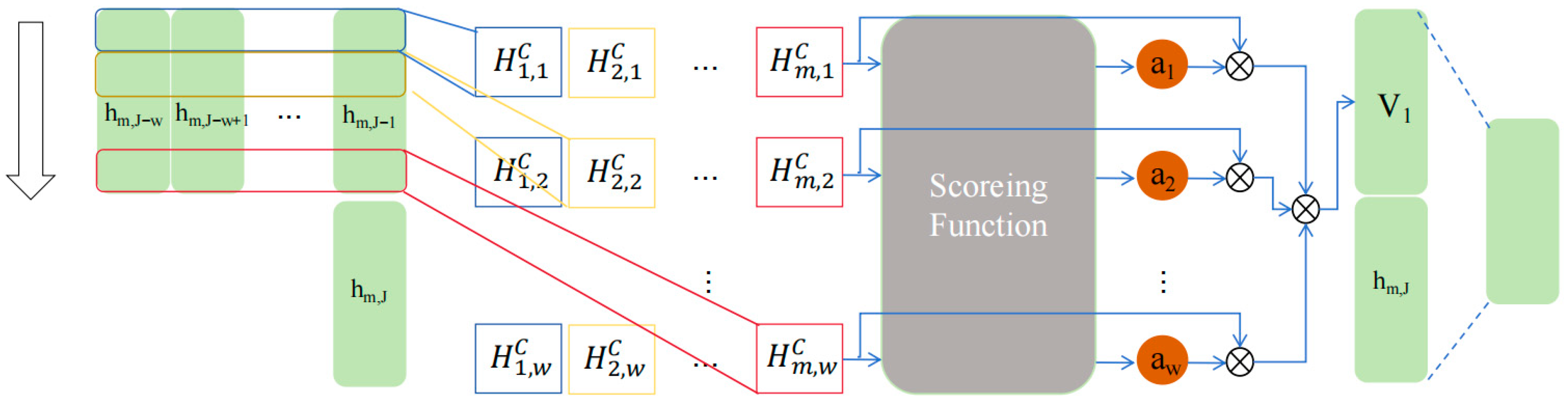
Spatio-temporal Attention Module: This model integrates a spatio-temporal attention mechanism, aiming to effectively capture the complex spatio-temporal characteristics of ocean data, thereby enhancing the accuracy of the filling results.
The structure of the remaining part of this article is as follows: The second part introduces traditional methods for marine data interpolation, including conventional machine learning methods and techniques based on Generative Adversarial Networks (GANs). The third part analyzes the network structure and principle of 3D-STA-SWGAIN. The fourth part discusses the data sources, experimental scenarios, and results. Finally, the conclusion section summarizes the method proposed in this article and outlines potential directions for future research.

2. Preliminary Knowledge

This section provides a detailed introduction to traditional interpolation methods, machine learning-based approaches, and techniques based on GANs used for interpolating marine dynamic environment parameters.

2.1. Imputation Methods for Marine Data Based on Traditional Interpolation Algorithms

At present, missing data completion based on sensor devices can be divided into two categories. Traditional missing data repair methods utilize the numerical correlation of adjacent time nodes and numerical simulation to construct data interpolation models.
Reynolds et al. [17] completed the data repair of the global daily average sea surface temperature (SST) product based on a time window by using the linear fitting method (LFM) model to fuse multi-source satellite data. Bilgili et al. [18] used the Seasonal Autoregressive Integrated Moving Average Model (SARIMA) to predict the missing sequence of SST in the eastern Pacific, and the Root Mean Square Error (RMSE) was reduced by 22% compared with the LFM model. Alvera-Azcarate et al. [4] introduced the time covariance matrix by using the Data Interpolating Empirical Orthogonal Function Decomposition (DINEOF) to iteratively optimize the missing spatio-temporal values and applied it to the MODIS chlorophyll concentration data completion. Sugiura N et al. [19] combined a four-dimensional variational assimilation model with the Ocean General Circulation Model (OGCM) and formalized the observation operator in data assimilation based on features extracted from the integrals contained in the ocean vertical profiles observed by the Array for Real-Time Geostrophic Oceanography (Argo) buoys. Liu et al. [20] utilized a cascaded temporal attention module to capture features at the hourly, daily, and monthly scales, and completed the imputation of missing data in ocean time series using Hybrid Coordinate Ocean Model (HYCOM) data and satellite observations.
However, highly complex numerical computations face numerous limitations, which hinder the popularization and application of numerical models; interpolation methods usually require the known data to follow a specific distribution and often fail to achieve satisfactory results for the irregularities commonly found in current marine data, presenting the problem of poor adaptability.
To address the limitations of statistical-based imputation methods, several imputation techniques grounded in traditional machine learning are discussed below. Feng et al. [21] proposed a novel data estimation method based on node clustering and genetic programming to estimate missing sensor data in wireless sensor networks, using genetic programming to mine the relationships among nodes within the same cluster. Zheng Qingyu et al. [22] employed hierarchical clustering to categorize data with different features, and to address the imbalance and sparsity of SST, combined variational autoencoders with deep learning regression networks and applied them to data completion, successfully alleviating the imbalance problem of samples. Due to the harsh marine environment, it is not uncommon for large amounts of data to be missing in certain areas during the data collection process [23]. Diouf et al. [24] proposed a method for completing large amounts of missing values. This method utilized preprocessing measures to decompose the dataset into continuous small parts, then used multi-criteria decision analysis to select a part of the data representing the entire fragmented dataset, and expanded the missing dataset by creating artificial missing data at different percentages and performing imputation using different machine learning techniques, achieving ideal results in meteorological data completion processing.

2.2. Imputation Methods for Marine Data Based on Traditional Machine Learning

As a core technical branch of artificial intelligence, deep learning, with its outstanding advantages in feature extraction and complex nonlinear relationship modeling, has been widely applied in the field of marine three-dimensional observation, providing a new technical path for enhancing the efficiency of marine three-dimensional observation [25,26,27]. Zihan Zhao et al. [28] employed the three-dimensional spatial interpolation technique of linear radial basis function (RBF-Linear) to conduct high-precision interpolation on the summer dissolved oxygen (DO) distribution collected by sensors in the Bohai Sea region of China. The root mean square error of the experimental results was ≤0.3 mg/L, and for the first time, the interannual variation pattern of the double hypoxia core area at the Bohai Sea mouth was revealed. Ao Li et al. [29] combined the marine dynamics dataset with the random forest algorithm to develop a new spatio-temporal interpolation method for chlorophyll-a (Chl-a) concentration in the South China Sea. By correlating spatio-temporal features, they achieved high-precision reconstruction of Chl-a concentration in missing areas, reducing the model error rate by 28% compared to traditional methods. In recent years, data-driven machine learning methods have begun to be applied in the field of missing data repair. These methods can automatically learn patterns directly from historical data to complete the missing parts of the data and show better results than traditional numerical calculations, effectively addressing the shortcomings of traditional methods. Current research indicates that deep learning techniques exhibit higher universality and effectiveness in addressing spatial completion problems.
However, the accuracy of deep learning models with a single network structure is not ideal, and their performance is highly dependent on the selection and tuning of hyperparameters. Chi et al. [30] utilized Two-Stream Long Short-Term Memory (TS-LSTM) to construct time-dynamic daily Arctic Sea ice data for the National Ice and Snow Center (NISC) SIC data using a perception loss-based TS-LSTM for sequence-to-sequence data completion. Wang et al. [31] embedded the time derivative term of the heat diffusion equation in the loss function on the basis of the physical information neural network to complete the time series strategy of sea surface data, reducing the time continuity error by 37%. Qin Mengjiao et al. [32] comprehensively considered temporal and spatial characteristics and proposed a multi-view learning (MCMVL) method based on matrix completion to fill in the missing values in buoy monitoring data, thereby enhancing the model’s imputation capability. Han Bin et al. [33] utilized a Graph Attention Network (GAN) to dynamically obtain the temporal and spatial information about ocean remote sensing data, encoded the spatio-temporal data through a global grid model, and combined static graph neural networks, neighborhood grid computation, and temporal evolution units, which could learn semantic, spatial, and temporal knowledge. This method performed well in spatio-temporal entity and relationship prediction tasks and was suitable for modeling the spatial correlation of ocean remote sensing data. Liu et al. [34] used a multimodal Transformer to fuse satellite remote sensing data such as Sea Surface Temperature (SST), Sea Surface Height (SSH), Argo buoys (temperature and salinity profiles), and reanalysis data (such as ECCO2), successfully reconstructing mesoscale eddy structures. Despite the significant progress made by these methods in addressing missing data problems, both traditional interpolation methods and machine learning-based data completion algorithms suffer from low completion accuracy, excessive reliance on historical data, poor applicability to real marine environments, and limitations to 2D planes.
The complex spatial characteristics of three-dimensional velocity fields make it difficult for traditional methods to accurately capture their complex time-varying and space-varying features. In contrast, GANs have shown considerable potential in marine data imputation.

2.3. GAN and SGAIN

The generative adversarial imputation algorithm [35] can interact with the environment in real time and update information. This characteristic determines that the generative adversarial network algorithm is suitable for dealing with marine environmental problems with time-varying and space-varying characteristics. The basic architecture of the generative adversarial network (GAN) consists of two main components: the Generator (G) and the Discriminator (D). The task of the generator is to generate new samples that are as close as possible to the distribution of real data, while the discriminator is responsible for distinguishing the generated samples from the real training data. During the adversarial training process, the generator constantly attempts to generate data that is difficult to identify as fake samples to deceive the discriminator; at the same time, the discriminator continuously improves its ability to distinguish real samples from generated samples. Through this mutual adversarial process, the model can eventually generate high-quality new data.
Slim-GAIN [36] is an advanced algorithm for the completion of spatio-temporal multivariate data, particularly suitable for the restoration of complex three-dimensional time series data such as ocean current fields and meteorology. Its algorithmic process is shown in Algorithm 1 as follows:
Algorithm 1 Slim-GAIN Algorithm Flow
1:  Input: Dataset X with missing values; mask matrix M; random noise distribution N;
2:  Parameter: Small-batch samples mb; Generator loss hyperparameters a: Number of iterations n int e r ;
3:  Output: The interpolated dataset y i
4:  Initialize the initial state M ← mask(X): Set each missing value to 0, and 1 otherwise.
5:  For  n int e r ← 1, n int e r do
6:   Draw mb samples from X: x ˜ ( j ) j = 1 m b
7:   Draw mb samples from m: m ˜ ( j ) j = 1 m b
8:   Draw mb independent and identically distributed samples from N and add random noise: n ˜ ( j ) j = 1 m b
9:   For j = 1, mb do
10:      z ˜ ( j ) m ˜ ( j ) x ˜ ( j ) 1 m ˜ ( j ) n ( j ) x ¯ ( j ) G z ˜ ( j ) , m ˜ ( j )
11:   End for
12:   Generator optimization, using Adam or RMSprop or SGD to update D
13:    θ D 1 m b m b j = 1 L D D x ˜ ( j ) , D x ˜ ( j ) , m ˜ ( j ) .
14:   Discriminator optimization, update G using Adam or RMSprop or SGD.
15:    θ G 1 m b m b j = 1 L G D x ¯ ( j ) , m ¯ ( j ) + α m b m b j = 1 L M S E x ˜ ( j ) , x ˜ ( j ) , m ˜ ( j ) .
16:   End for
17:   Z M X ( 1 M ) N X ¯ G ( Z , M ) X ^ M X ( 1 M ) X ¯
18:  Save the generated data that is closest to the real distribution and output it: y i

2.4. Attention Mechanism

In view of the complexity of the marine environment, adaptive attention algorithms can better capture information. The attention mechanism algorithm has intelligent adjustment capabilities, providing a certain basis for the adaptive adjustment of feature weights and the capture of periodic and spatial change trends.
The spatio-temporal attention mechanism [37] is an innovative deep learning technique that effectively focuses on the most representative and influential parts of the data by adaptively allocating weights to different time points and spatial locations, thus becoming a powerful tool for capturing temporal and spatial information. Specifically, the spatio-temporal attention mechanism can dynamically adjust the model’s focus on each spatio-temporal unit, enabling the model to more flexibly capture key information and comprehensively aggregate the mutual influence and interaction of features at different spatial and temporal scales, thereby enhancing the model’s ability to recognize and predict complex spatio-temporal patterns. In meteorological analysis, the spatio-temporal attention mechanism enables the model to focus on critical time periods and regions that play a key role in weather changes, such as the key turning points of typhoon paths or areas with concentrated heavy rainfall, thereby improving the accuracy of forecasts.
S = S i g m o i d ( p r o d u c t + b n )
S normalized = exp ( S max ( S , axis = 1 ) ) t exp ( S max ( S , axis = 1 ) ) .
Here, S is obtained by adding a biased bn to the calculation result “product” and activating it through the Sigmoid function. “product” is the batch dot product result, used to represent the correlation between time series.

3. Proposed Method

In this section, we will systematically introduce the structure and principle of the model. First, we will elaborate in detail on the implementation methods that support the model. Then, we will delve into the overall framework and the implementation details of its core components. Finally, we will analyze the key modules in the model one by one, such as the spatio-temporal attention mechanism and the convolutional neural network, explaining the reasons for their inclusion and their specific implementation mechanisms.

3.1. Framework

We focus on the interpolation of 3D ocean current field data, addressing 3D features. Let the ocean current field be a d-dimensional space X = ( X 1 , X 2 , , X d ) . Each { X i } d i = 1 has a non-missing value in { X i } d i = 1 , and the missing values in { X i } d i = 1 are replaced by random values. Suppose a random variable x = x 1 , x 2 , , x d represents the velocity component of a three-dimensional flow field data, and its value is determined by the distribution P X . Meanwhile, define a random variable M = M 1 , M 2 , , M d composed of 0 and 1 as a mask vector to mark the observation status.
For each dimension k 1 , 2 , , d , define a random variable x = ( x 1 , x 2 , , x d ) in the observation space. Here, x k only retains the non-missing parts, and the missing parts are indicated by the symbol X: Additionally, we assume a random variable M = M 1 , M 2 , , M d , composed of 0 s and 1 s, which serves as the mask tensor.
x k = x k , i f   M k = 1 X , o t h e r w i s e
Here, lowercase letters denote instantiations of random variables, and ‘1’ represents a vector in which all elements are 1, i.e., a vector of all 1 s.
The ultimate goal is to approach the true data distribution P(X) through adversarial training, accurately impute the missing values, and thereby capture the spatial correlation and inherent uncertainty of the flow field data. By generating results through multiple samplings, the confidence range of the imputed values can be further quantified.
This chapter proposes a 3D generative adversarial completion network for addressing the common problem of missing flow field data in the process of 3D observation of ocean currents. It is applicable to data completion tasks of different patterns and different degrees of missing data. This network can capture the spatio-temporal relationship of ocean current fields and complete the incomplete three-dimensional flow field data. Its core components include the comprehensive application of spatio-temporal attention mechanism, generative adversarial interpolation network, and penalty function.
The overall architecture of the proposed model 3D-STA-WSGAIN is shown in Figure 1. Here, “3D” indicates that the network structure of the model is suitable for the completion of stereoscopic ocean current observation data. In this network, both the input and output of the generator and the discriminator are four-dimensional tensors. For this chapter, it is difficult to visually present the complex structure of four-dimensional tensors with a planar schematic diagram. Therefore, a three-dimensional form was adopted in the schematic diagram to simplify the representation.
In the generator and critic, the missing data are first masked to form a complete input. The spatio-temporal attention mechanism module is utilized to learn the spatio-temporal relationships among the known data and weigh the spatio-temporal importance of the input data. Through the weighted data, the network can better focus on and utilize the relevant information in the known data, thereby making the completion results of ocean current field data more accurate.
To enhance the authenticity of the generated samples, the critic measures the distribution difference between the generated samples and the real flow field data through the Wasserstein distance, maximizing the Wasserstein distance between the real samples and the generated samples, and introduces a Gradient Penalty (GP) term to improve the training stability.
By designing the input and output of the ocean current field (time × depth × latitude × longitude), the neural network can more effectively extract the three-dimensional global features of the complex ocean current field. This design not only considers the spatial dimensions but also combines the information about the temporal dimension, thereby comprehensively capturing the dynamic changes in the ocean current field. Compared with the traditional methods that only rely on spatial features, 3D-STA-WSGAIN can better reflect the spatio-temporal correlation of the ocean current field and significantly improve the accuracy of data completion.
By introducing the spatio-temporal attention mechanism, the model can dynamically adjust the importance of different positions and time points in learning the 3D ocean flow field. This makes the model more flexible and robust when dealing with different missing patterns and missing rates. For example, in cases where there is a large area of missing data in certain depth layers or nodes, the attention mechanism can more accurately estimate the missing values by learning the spatial and temporal relationships.

3.2. Core Modules

The implementation of the 3D-STA-SWGAIN model mainly relies on the following four key components: generative adversarial network, attention mechanism module, gradient penalty module, and loss function.

3.2.1. The Main Model of 3D-STA-SWGAIN

(1)
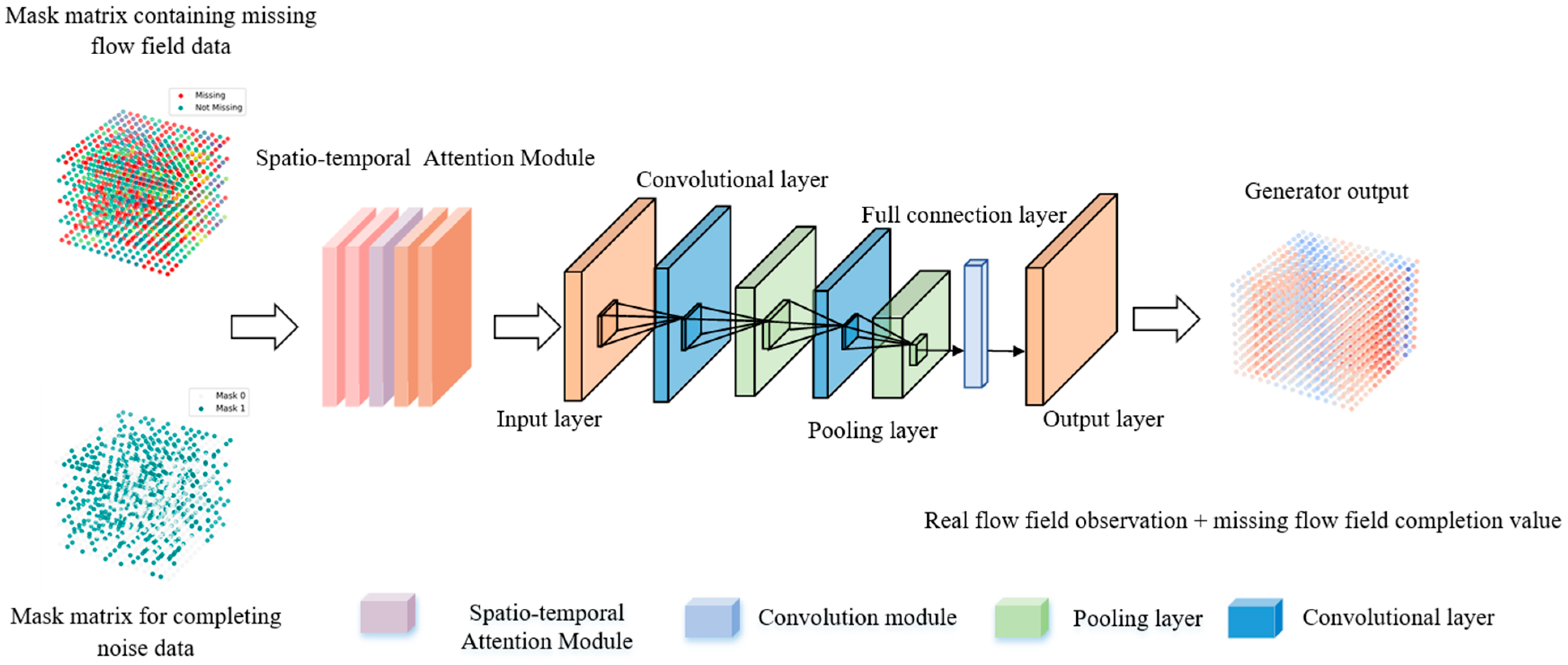
Generator: The generator in 3D-STA-SWGAIN is composed of a convolutional neural network based on the spatio-temporal attention mechanism, which can capture the spatial and temporal dependencies of ocean flow field data. It takes incomplete ocean current field data as input, with the goal of generating missing values through adversarial learning that are consistent with the distribution of real ocean current field data. The interpolation process of the generator can be expressed by Equations (4) and (5).
x = M X ( 1 M ) x
G ( x , M ) X
Among them, M represents the mask tensor, x represents the incomplete ocean current data with missing values, and X is the complete data after filling. The generator is responsible for generating completed data similar to the distribution of real data based on the input random noise vector. In the task of completing the three-dimensional ocean flow field, the generator adds noise ϵ ( t ) and resamples it in each iteration, thereby making the input 5 of the generator dynamic. The symbol denotes indicates the element-wise multiplication of the four-dimensional tensor. During the training process of the generator, the retention of the original ocean current field information is achieved, that is, the existing observed values are completely retained without introducing noise interference; for the missing parts of the ocean current field observed values, uncertainty modeling is introduced, and the missing values are filled with random noise. The generator needs to learn a reasonable data filling pattern for the ocean current field from the noise distribution, laying the foundation for adversarial training; dynamic noise makes it impossible for the critic to distinguish the generated ocean current field data through a fixed pattern, promoting the balanced optimization of the generator–critic.
The objective of the generator is to minimize the Wasserstein distance. Its loss function is to increase the score of the generated samples, making them closer to the real distribution. The loss function of the generator is as follows:
L C = E z p z [ C ( G ( z ) ) ]
In the formula, C represents the critic, and G(z) represents the pseudo-samples generated by the generator based on noise z. p z is the prior distribution of the noise. The optimization objective of the generator is to minimize the weighted sum of the adversarial loss and the reconstruction loss:
L G = E [ C ( X ^ ) ] + β M G ( X ˜ , M ) X 2  
Among them, the weight β controlling the reconstruction loss,   represents element-wise multiplication.
When training the model, it is necessary to ensure that the distribution is as similar as possible to that of the real flow field samples, and to gradually enhance the generator’s ability to simulate real flow field samples through cyclic alternating training.
(2)
Critic: As shown in Figure 2, the Critic in 3D-STA-SWGAIN adopts a convolutional neural network architecture enhanced by a spatio-temporal attention mechanism. The key difference from the generator lies in the input form: the critic receives a combination of the data output by the generator and the mask matrix. Its core objective is to learn the global features and spatio-temporal relationships of multiple sets of 3D ocean current field data, thereby accurately distinguishing real data from the data generated by the generator.
In traditional GAIN, the output of the generator is composed entirely of either real data or synthetic data. However, in 3D-STA-SWGAIN, the generator produces a mixture of real values and imputed values. Therefore, the function of the critic changes to evaluating the probability that each data point generated by the generator belongs to the real ocean current field data.
The critic measures the distribution difference between the generated samples and the real flow field data through the Wasserstein distance, maximizes the Wasserstein distance between the real samples and the generated samples, and introduces a gradient penalty term (GP) to enhance the training stability. Its loss function is shown in Equation (8).
  L C = E x ~ P r [ f ( x ) ] + E x ~ P g [ f ( x ) ] + λ gradient   penalty
Among them, P r represents the true distribution, P g is the distribution of the generator, f ( x ) is the output of the critic, λ is the coefficient of the gradient penalty.

3.2.2. Spatio-Temporal Attention Mechanism Module

To effectively capture the interaction of ocean current velocity in continuous space and time, a spatio-temporal attention mechanism is adopted to extract spatio-temporal features at specific scales. The spatio-temporal attention mechanism is a technology capable of simultaneously capturing temporal and spatial data. When dealing with spatio-temporal data, it can not only capture the spatial features between neighboring ocean currents but also the temporal features of the same phase and can simultaneously consider the attention weights of the spatial and temporal dimensions. The spatio-temporal attention mechanism includes attention to data in the temporal and spatial dimensions. The temporal dimension usually reflects the dynamic process of data evolution over time, while the spatial dimension reflects the interrelationships between different locations or nodes. The spatio-temporal attention matrix is used to calculate the relationship between different positions in the spatial dimension, to weigh the input features. The scoring function is used to determine the weight of the temporal information and obtain the final output information based on the size of the weight. Specifically, Equations (9) and (10) are expressed as follows:
S e = Sigmoid ( product + b e ) .
S normalized - 1 = exp ( S e max ( S e , axis = 1 ) ) t exp ( S e max ( S e , axis = 1 ) ) .
Here, S e is obtained by adding a biased be to the calculation result “product” and activating it through the Sigmoid function “product” is the batch dot product result, used to represent the correlation between time series.
Specifically, the structure of the spatio-temporal attention mechanism is shown in the Figure 3. First, for each depth of data, features are extracted from the spatial dimension, and spatial attention weights are extracted, followed by a convolution operation. Then, on this basis, temporal features are extracted and spatio-temporal attention weights are calculated. The processed feature vectors undergo a convolution operation to generate spatio-temporal weight coefficients. The Sigmoid activation function is used to obtain the distribution of weight coefficients, and finally, the allocation coefficients for each spatial position are obtained, indicating the importance of that position.
In the generator and critic, we first mask the missing data to form a complete input. Then, the spatio-temporal attention mechanism module is used to learn the spatio-temporal relationships among the known data and weigh the spatio-temporal importance of the input data. Through the weighted data, the network can better focus on and utilize the relevant information in the known data, thereby making the results of ocean current field data completion more accurate.

3.2.3. Gradient Penalty Module

In view of the spatio-temporal continuity and complex physical laws of ocean current field data, this study innovatively introduces the GP mechanism in the optimization of the SWGAIN model, effectively addressing the problems of limited network capacity and overfitting caused by traditional weight pruning methods. Compared with the hard constraints on the parameter space of the critic imposed by conventional weight pruning, GP achieves better Lipschitz continuity control through flexible regularization, which is particularly important for maintaining the spatial correlation of physical properties in ocean current fields.
The design of the GP term fully considers the particularity of the ocean current field data generation task: the calculation of the penalty term involves the gradient calculation of the interpolated samples between real ocean current field samples and generated ocean current field samples.
GP = α x + 1 α G z
x represents the real sample, and G z represents the generated sample. By calculating the gradient norm x ^ f ( x ^ ) 2 of the critic on the interpolated samples, it ensures that it strictly satisfies the 1-Lipschitz condition. This gradient constraint mechanism for the transition zone can significantly enhance the continuity of the generated flow field in sensitive areas such as the vortex edge and frontal interface, avoiding the pseudo-vortex or false streamline phenomena commonly seen in traditional methods. Secondly, a dynamic penalty weight λ is used to adaptively adjust the gradient deviation. When x ^ f ( x ^ ) 2 deviates from the unit norm, the L2 penalty term λ x ^ f ( x ^ ) 2 1 2 is used to precisely control the gradient magnitude. This flexible constraint not only retains the network’s ability to express complex flow field features but also ensures the numerical stability of the training process.
The gradient penalty function is reflected in the loss function of the critic, and the gradient penalty term is expressed as follows:
GP = E x ^ ~ P interp λ x ^ f ( x ^ ) 2 1 2
Experiments show that this gradient penalty mechanism demonstrates dual advantages in the task of ocean flow field completion: on the one hand, by constraining the Lipschitz continuity of the critic, it effectively suppresses the gradient oscillation phenomenon during the training process; on the other hand, the gradient calculation strategy based on physical space interpolation can accurately capture the dynamic transition features between the real flow field and the generated area [37]. In the South China Sea flow field data completion experiment, the mean absolute error (MAE) of the three-dimensional ocean flow field was reduced by 93.56% compared with the traditional interpolation method, providing an important technical guarantee for building a high-fidelity ocean flow field generation model.

3.2.4. Loss Function

Compared with the traditional loss function measurement methods, the Wasserstein distance more comprehensively reflects the similarities and differences between the distributions of real samples and generated samples. It not only quantifies the optimal transportation cost between data distributions but also incorporates the distances moved during the transformation process. Moreover, it explicitly models the spatial correlations of ocean dynamic structures such as vortices and fronts by precisely measuring the distribution differences between real and generated flow fields in the probability space [38].
Maintain the spatio-temporal continuity of ocean flow fields. By calculating the geometric distance weights between flow field data points, it effectively maintains the continuous distribution characteristics of flow velocity and direction in three-dimensional space, compatible with multi-scale features of ocean flow fields. It can simultaneously capture local turbulence details and global flow velocity transmission characteristics [39], enhance physical rationality. The gradient penalty term constrains the Lipschitz continuity of the critic, avoiding physical paradoxes such as abnormal vorticity and mass imbalance that occur when traditional networks train high-dimensional flow field data [40].
In the 3D-STA-WSGAIN model, we adopt the Wasserstein distance as the core loss function and combine it with the gradient penalty (GP) mechanism to achieve stable training. This design is of particular significance for the completion of ocean flow field data.
The formula and related information about the Wasserstein distance can be summarized as follows:
W ( P r , P g ) = sup f L 1 E x ~ P r [ f ( x ) ] E x ~ P g [ f ( x ) ]
Among them, ( P r , P g ) represents the set of all joint distributions between the real flow field samples and the generated flow field samples. The Wasserstein distance is obtained by calculating the difference between the two samples and the expected value of the distance under the joint distribution E x ~ P r [ f ( x ) ] E x ~ P g [ f ( x ) ] .
The formula of the loss function is shown as follows:
L C = E X ^ ~ G ( X ˜ , M ) [ D ( X ^ ) ] E X ~ P ( X ) [ D ( X ) ] + λ E α ~ U ( 0 , 1 ) ( X ˜ D ( α X ˜ + ( 1 α ) X ^ ) 2 1 ) 2
Among them, G ( X ˜ , M ) represents the distribution of the features of the real flow field data, α indicates sampling from the uniform distribution U 0 , 1 , and α is the distribution of random noise. The proposed loss function introduces additional gradient penalties to further stabilize the training process.

3.3. Implementation Procedures

The objective of this paper is to model the data distribution through the 3D-STA-WSGAIN framework and generate interpolation results consistent with the real distribution by leveraging the adversarial training mechanism. Through multiple adversarial iterations and sampling, the quality of the generated data is gradually optimized, ultimately achieving high-quality completion of flow field data [41].
The specific implementation process of the proposed 3D-STA-WSGAIN framework can be summarized as follows:
Step 1: Input: Dataset X with missing values; Mask matrix M; Random noise distribution N;Set parameters: Mini-batch sample mb; Generator loss hyperparameter a; Number of iterations n int e r ; Critic loss hyperparameter lambda; Number of times to train the discriminator n c r i t i c ;
Step 2: Initialize the initial state M ← mask(X): Set each missing value to 0, and 1 otherwise;
Step 3: Input the ocean current data into the spatio-temporal attention module to dynamically allocate weights;
Step 4: Generator optimization, using Adam or RMSprop or SGD to update D;
Step 5: Critic optimization, update G using Adam or RMSprop or SGD;
Step 6: Save the generated data that is closest to the real distribution and output it.

4. Experiments

This paper mainly introduces the source of experimental data and the experimental results to evaluate the performance of the proposed 3D-STA-SWGAIN algorithm. By comparing the differences in Mean Absolute Error (MAE), Mean Squared Error (MSE), etc. between the cubic spline interpolation method, the method based on adversarial generative imputation network, the method based on KNN, etc., the superiority of the proposed 3D-STA-SWGAIN algorithm based on spatio-temporal attention is verified. At the same time, to verify the universality of the algorithm, it was validated in the South China Sea environment. The area circled by the black box in Figure 4 is the source of the experimental data for this experiment.

4.1. Datasets and Settings

To verify the performance of the 3D-STA-Slim-WGAIN algorithm, the following flow velocity datasets were adopted for experiments. The experimental part of this paper utilized the real-time analysis flow field data of the Northwest Pacific provided by the National Marine Data Center. These data were reconstructed from the water three-dimensional flow field based on the sea surface velocity and sea surface height data from the National Satellite Ocean Application Center and international public sources. This includes the SST dataset released by the National Oceanic and Atmospheric Administration of the United States [42] (https://psl.noaa.gov/map/clim/sst.shtml, accessed on 23 April 2025), the AVISO satellite altimetry dataset [43], and the CCMP dataset released by the National Centers for Environmental Prediction of the United States [44].
Meanwhile, the reconstructed field was assimilated and corrected using real-time or quasi-real-time data from international public sources and the center’s observation and monitoring (https://mds.nmdis.org.cn/pages/home.html, accessed on 23 April 2025). It covers the sea area ranging from 99° E to 150° E and 10° S to 52° N, with a horizontal spatial grid resolution of 0.125° and standard layer division in the vertical direction.
Based on this, data from the South China Sea region was extracted, with the latitude and longitude range being 13.0° N–16.5° N and 115.5° W–119.0° W, respectively. The final data dimension obtained was (1275, 25, 30, 30), where 1275 represents the total amount of time series data, that is, a total of 1275 data points were selected in the time dimension, 25 represents the number of depth layers of the ocean, with each layer being 100 m, and (30, 30) represents the latitude and longitude range of the velocity data. The schematic diagram of the experimental location is shown as such. The dataset mainly includes reanalysis data information about USSV and VSSV. A schematic illustration of the experimental location is provided in Figure 4 and Figure 5.

4.2. Baseline Models for Interpolation of Ocean Current Field Data

In the experimental section of this paper, we introduce the 3D-STA-SWGAIN model, which is constructed using the GAN neural network library. To evaluate the effectiveness of the proposed model under different missing data patterns and missing rates, we conducted comparative experiments involving four other models. The detailed information about these models is as follows:
(1)
Cubic Spline Interpolation: It is a commonly used interpolation method for constructing smooth curves between known data points. By fitting cubic polynomials between adjacent data points, it ensures that the entire interpolation curve has continuous first and second derivatives at these points, thereby guaranteeing the smoothness of the curve.
(2)
Deep Matrix Factorization (DMF): This is a novel imputation technique that improves upon traditional matrix factorization methods. Its key feature is the ability to handle data with nonlinear structures. By leveraging deep learning techniques, this method can more accurately learn the features and structures of the data, thereby achieving more effective imputation of missing values.
(3)
Transformer deep learning network: A deep learning model based on the self-attention mechanism, its core advantage lies in the parallel processing of long sequence data and the capture of global dependencies, which has completely transformed the traditional RNN/LSTM model’s approach to sequence modeling.
(4)
3D-SGAIN: This is a method based on GAN for imputing missing data. It estimates the missing values by training a generator and a discriminator.
Given that the above algorithm mainly focuses on interpolating 2D flow field data, we first convert the 3D flow field data into a 2D data format and then proceed with the data completion processing.

4.3. Evaluation Indicators for Interpolation of Ocean Current Field Data

To evaluate the predictive performance of different models, four assessment metrics are selected for quantitative evaluation: Mean Absolute Error (MAE), Mean Squared Error (MSE), Root Mean Square Error (RMSE), and R-squared (R2), as detailed below.
MAE is the average of the absolute errors between the generated sample values of the ocean current field and the true values, and it is used to measure the accuracy of the model.
MAE = 1 N i = 1 N x p r e , i x a c t , i
MSE is a commonly used evaluation metric in machine learning and statistics, which is used to measure the difference between the generated flow velocity sample values and the true values, and it is defined as follows:
MSE = i = 1 N ( x a c t , i x p r e , i ) 2 N .
RMSE quantifies the overall deviation degree of the model’s completion results by calculating the square root of the error between the generated velocity field and the true velocity field, reflecting the prediction accuracy of the model:
RMSE = 1 N i = 1 N ( x a c t , i x p r e , i ) 2 .
R2 represents the proportion of the variability of the real data that can be explained by the model’s predicted values, and it can measure whether the model maintains the spatial-temporal correlation and dynamic patterns of the flow field:
R 2 = 1 SS res SS tot
In the formula, x a c t , i represents the true value of the flow field in the i-th missing area; x p r e , i represents the interpolation value of the i-th missing area; N indicates the total number of missing flow field data samples. SS res is the sum of squared residuals, and SS tot is the total sum of squares.

5. Discussion

In the experiment, multiple sets of experiments were conducted under different missing rates for the common missing scenarios of ocean current field data.
Specifically, Pattern (a) represents the scenario of randomly missing flow field data. Pattern (b) reflects the phenomenon of data absence caused by cloud cover in satellite observations, which may result in the loss of certain horizontal layers within the oceanic flow field. Finally, Pattern (c) illustrates a block-type missing pattern resulting from sensor array malfunctions. These missing patterns are designed to simulate various scenarios of data loss, thereby enabling a comprehensive assessment of the effectiveness and robustness of methods for handling missing data.

5.1. Experimental Analysis of Ocean Current Field Data Completion Under Different Modes

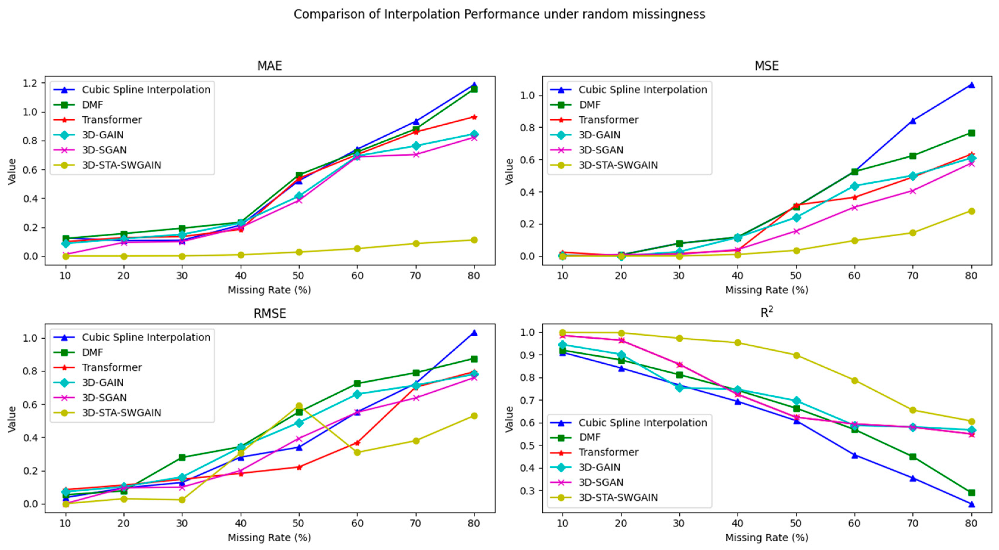
5.1.1. Pattern (a) Random Missing Pattern of 3D-STA-SWGAIN

Based on the above experimental data, experimental scenarios, comparison test models, and evaluation indicators, this section divides different missing rates according to the random missing pattern. The comparison results with the benchmark model are shown in the following figure, and the visualization results are shown in Table 1 and Figure 6.
This study focuses on the problem of missing data in three-dimensional ocean flow fields and systematically compares the performance of traditional interpolation methods and deep learning models in data reconstruction tasks. The research results show that in cases of low missing data rates, traditional interpolation methods can maintain the local continuity of ocean flow fields relatively well and are suitable for small-scale data repair tasks. However, when the missing data rate is high (for example, over 20%), the limitations of traditional methods gradually become apparent, with their reconstruction errors significantly increasing, reaching up to 120% at most. This phenomenon is mainly attributed to the difficulty of traditional methods in capturing the complex spatio-temporal dynamic characteristics of ocean flow fields, especially when dealing with large-scale and nonlinear missing data patterns, their modeling capabilities are particularly insufficient.
To address the aforementioned issues, this study proposes a novel model based on deep learning. By integrating spatio-temporal attention mechanisms and penalty constraint strategies, this model significantly enhances its adaptability to scenarios with high missing rates. Specifically, under conditions of 30% to 60% missing rates, the proposed model can reduce the mean square error of horizontal flow velocity by 32.7%, demonstrating clear superiority over the traditional GAIN. This improvement is attributed to several key factors: Firstly, the spatio-temporal attention mechanism can dynamically allocate weights, effectively capturing complex correlations at different temporal and spatial scales in ocean current fields; secondly, the introduced penalty constraints further enhance the model’s robustness to outliers and noise, ensuring the stability and reliability of the reconstruction results.

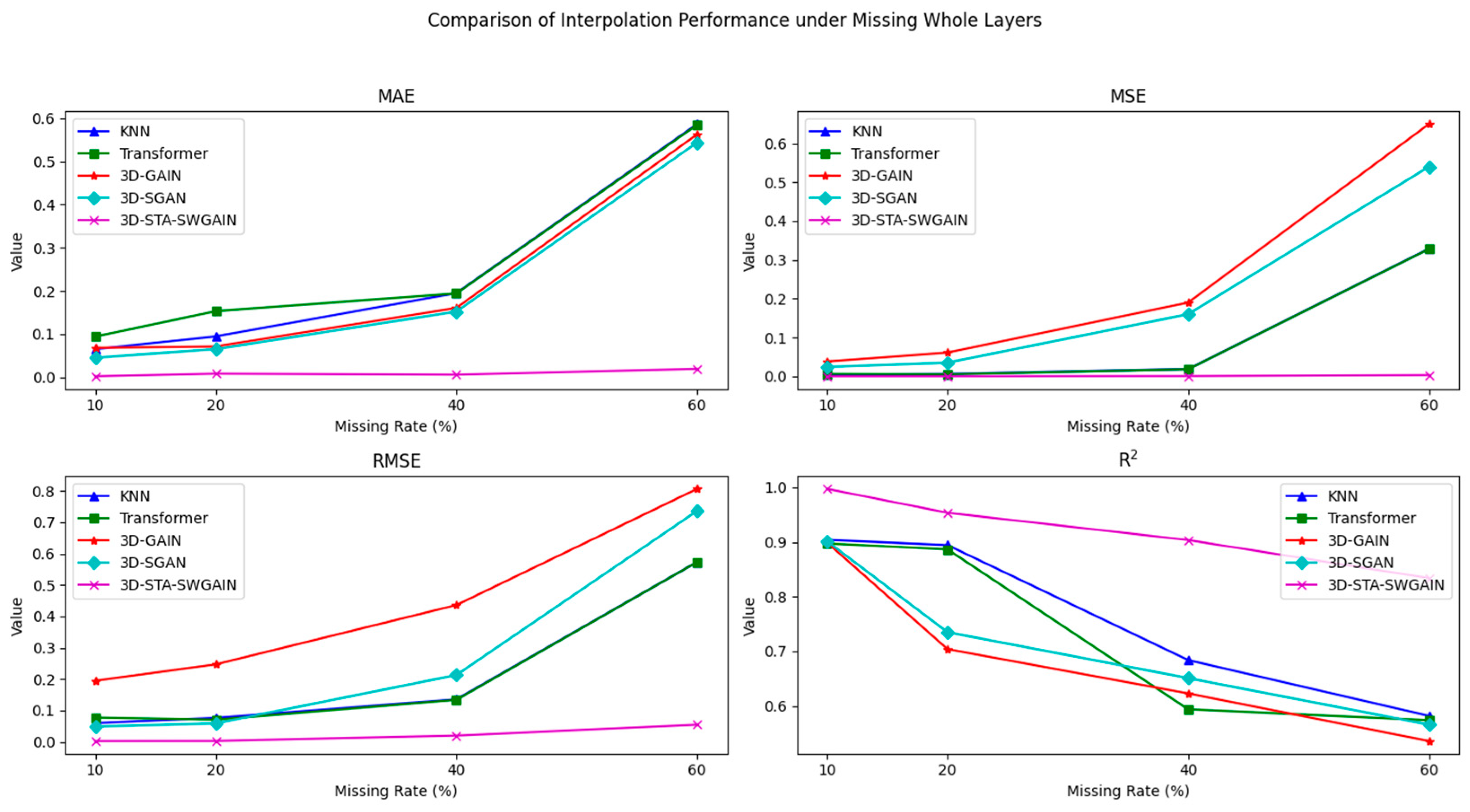
5.1.2. Pattern (b) the 2D Ocean Current Layer Missing Pattern Caused by Cloud Cover in Satellite Data of 3D-STA-SWGAIN

In response to the phenomenon of missing two-dimensional ocean current layer data in satellite data due to cloud cover, this study systematically compared the interpolation capabilities of different models in three-dimensional ocean current fields. This issue is of great significance in marine scientific research and practical applications, as cloud cover often leads to the incompleteness of satellite observation data, thereby affecting the understanding and prediction of ocean dynamic processes.The experimental results are shown in Table 2 and Figure 7.
Experimental results show that traditional methods have obvious limitations when dealing with missing two-dimensional flow layers. Specifically, due to their difficulty in effectively capturing the dynamic correlations between horizontal layers and the vector evolution rules across time steps, they exhibit significant errors in reconstructing missing data. For instance, when faced with missing data in cloud-covered areas, the flow direction error of traditional methods exceeds 60%, almost completely losing their reconstruction capability. This limitation mainly stems from the design characteristics of traditional methods: they usually assume that the changes in ocean flow fields are locally linear or static, while ignoring the complex nonlinear and spatio-temporal dynamic characteristics in ocean flow fields. Therefore, when dealing with large-scale or long-term sequence missing data, traditional methods often fail to provide reliable reconstruction results.
To address this issue, this study proposes a novel interpolation model based on the spatio-temporal attention mechanism. This model significantly enhances interpolation accuracy by integrating historical concurrent flow field features and dynamic constraints from adjacent layers. Specifically, the spatio-temporal attention mechanism can dynamically allocate weights, effectively capturing complex correlations at different temporal and spatial scales in ocean flow fields. For instance, it can flexibly adjust the focus on historical flow field features based on the context information at the current moment, while incorporating dynamic constraints from adjacent layers to mitigate the impact of missing data. This design enables the model to generate relatively accurate interpolation results even in the case of completely missing layers.
Experimental verification shows that, compared with the traditional 3D-SGAIN model, the interpolation model proposed in this study reduces the error in the horizontal flow vector direction by 95.56%. This significant improvement not only proves the effectiveness of the spatio-temporal attention mechanism but also demonstrates the model’s superior performance in handling complex ocean current field data. Moreover, the successful application of this model provides higher-quality data support for marine scientific research, which helps enhance the understanding of ocean dynamic processes and offers important technical support for practical application fields such as climate change prediction and marine resource development.

5.1.3. Pattern (c) Block-Shaped Missing Patterns Caused by Sensor Array Faults of 3D-STA-SWGAIN

Block-shaped missing data refers to the complete absence of data in a continuous spatio-temporal region, thus forming what is known as a “void”. This type of missing data usually has a certain spatial or temporal range, and its impact may extend to multiple related variables. For example, in ocean observation, sensor array failure is a common cause of block-shaped missing data. When a sensor or a group of sensors fail, the area they cover will be unable to provide valid observation data, thereby creating large areas of data blank. This situation is not uncommon in practical applications, especially in cases where data collection relies on satellite remote sensing or buoy networks.
When block-shaped missing data occur in ocean current fields, traditional data interpolation methods often struggle to handle them effectively. For instance, three-dimensional KNN interpolation, which is based on the weighted average distances from the nearest neighbors, assumes that the value of the target point is highly similar to its surrounding neighboring points. However, when dealing with block-shaped missing data, the effectiveness of this method significantly declines because the points within the missing area lack sufficient neighboring points for reasonable estimation. Additionally, although ordinary interpolation networks can utilize machine learning techniques to predict missing data, they still have obvious limitations when dealing with a high proportion of block-shaped missing data. Specifically, these methods usually have difficulty capturing the dynamic correlations between different cross-sections, and when the missing rate exceeds 60%, the error of the completed speed data may exceed 55%. The fundamental reason for this problem lies in the fact that ocean current fields themselves have complex spatio-temporal dynamic characteristics, and their changes are influenced by multiple factors, including wind stress and tidal forces. Therefore, relying solely on local information or static models for interpolation often fails to accurately restore the true flow field structure.The experimental results are shown in Table 3 and Figure 8.
In contrast, the model we proposed demonstrates outstanding performance and robust reliability when dealing with complex and extreme block-wise missing data problems. This advantage mainly stems from several key features in the model design. Firstly, the model can effectively learn and integrate spatial information from multiple time stamps, thereby establishing a more comprehensive data correlation. This cross-time-step learning ability enables the model to not only rely on the local information at the current moment but also fully utilize the patterns and rules in historical data, which is particularly important for solving problems of long time series or large-scale missing data.
In the task of interpolating ocean current field data, when the data of an entire layer is completely missing, traditional methods often struggle to generate reasonable predictions due to the lack of sufficient contextual information. However, our model can, to a certain extent, compensate for these missing data by integrating spatial features from adjacent layers and historical moments, thereby maintaining a high interpolation quality. This characteristic is of great significance in practical application scenarios, especially in satellite remote sensing or sensor network observations, where large-scale data loss due to equipment failure and other reasons is very common. As can be seen from the above experimental results, the effectiveness of this model in addressing the challenge of complex block-shaped missing data have been fully verified. It not only provides higher-quality data support for scientific research but also offers a reliable solution to the data integrity problem in the field of marine engineering applications.

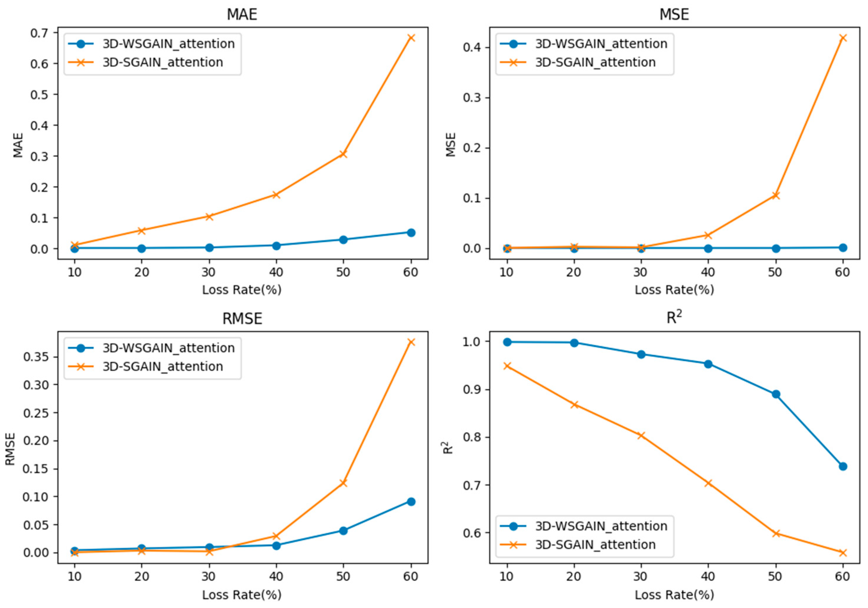
5.2. Ablation Experiments and Evaluation

To verify the effectiveness and significance of the key components in the proposed model in this paper, a series of ablation studies were conducted. During the training and evaluation phases, consistent experimental conditions were maintained to ensure fair comparisons. In the ablation tests, the spatio-temporal attention mechanism and the Wasserstein-GP loss function were excluded, respectively, denoted as “W/O U”, where “U” represents the specific component. Through these ablation experiments, the specific roles and contributions of these components in the model can be more clearly observed.
(1)
A comparative experiment on the impact of data completion results under models with and without spatio-temporal attention mechanism.
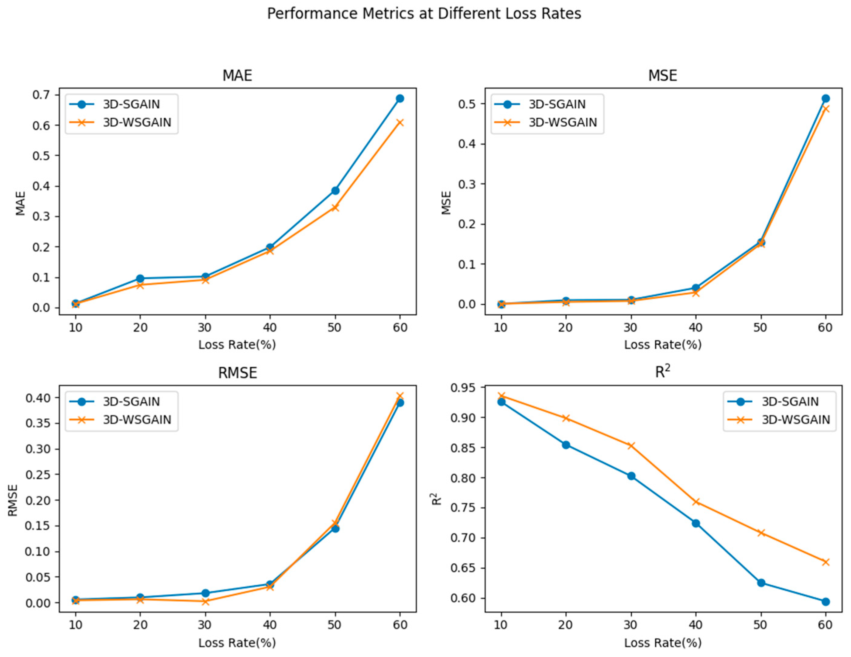
Without spatio-temporal attention mechanism (W/O 3D-SWGAIN-GP): Under the configuration of this ablation experiment, the spatio-temporal attention mechanism in the model was removed, and only the 3D-SWGAIN-GP model was retained. By comparing the performance of the model when the spatio-temporal attention mechanism is retained, the advantages of the spatio-temporal attention mechanism in handling the complex spatio-temporal data of three-dimensional flow fields can be more clearly highlighted, and the improvement effect of the spatio-temporal attention mechanism on the model performance can be explored.
As shown in Figure 9, the crucial role of the 3D-STA-SGAIN model in the complete modeling of ocean current field data is quite evident. Specifically, when the spatio-temporal attention mechanism is removed from the model (i.e., 3D-SWGAIN-GP is disabled, marked as W/O 3D-SWGAIN-GP), the model’s performance drops significantly. This decline is not only reflected in the obvious reduction in spatial pattern consistency between the completed field and the real field, but also in the significant increase in the average error quantification index. This result indicates that relying solely on traditional completion network modeling methods is difficult to effectively capture the complex and dynamic spatio-temporal characteristics in the changes in ocean three-dimensional current fields.
The changes in the three-dimensional flow field of the ocean are inherently highly nonlinear and uncertain, with extremely complex spatio-temporal dynamic characteristics. For instance, the ocean flow field may be influenced by multiple factors, including seasonal variations, local weather conditions, and broader climate phenomena such as El Niño or La Niña. The combined effect of these factors results in a high degree of spatio-temporal heterogeneity in the changes in the ocean flow field. Therefore, traditional completion methods often fail to fully account for these complex spatio-temporal relationships, leading to insufficient accuracy in the completion results.
In contrast, the spatio-temporal attention mechanism proposed in our model demonstrates significant advantages. By introducing this mechanism, the model can more accurately capture the spatio-temporal characteristics of the missing ocean current field data. The core of the spatio-temporal attention mechanism lies in its dynamic weight allocation capability, which can flexibly emphasize important spatio-temporal information according to the current prediction needs. For instance, in some cases, recent changes in the temporal dimension may be more important than distant correlations in the spatial dimension; while in other cases, information from spatially adjacent regions may play a dominant role. This flexible modeling approach enables the model to better adapt to the complex spatio-temporal dynamics in different scenarios, thereby significantly improving the accuracy and reliability of the completion results.
In conclusion, the experimental results fully verify the significant role of the spatio-temporal attention mechanism in dealing with missing three-dimensional ocean flow field data. This mechanism not only makes up for the deficiencies of traditional methods but also provides new ideas and directions for future research in related fields.
(2)
A comparative experiment on the impact of different loss function models on data completion results.
Without Wasserstein-GP loss function (W/O 3D-STA-SWGAIN): In this configuration, only the Wasserstein-GP loss function was removed while the 3D-STA-SGAIN model was retained. The purpose of this was to separately evaluate the impact of the Wasserstein-GP loss function on model performance. By observing the performance changes in the model in processing real flow field and interpolated flow field information in the absence of the Wasserstein-GP loss function, the key role of the Wasserstein-GP loss function in spatial feature extraction and the modeling of the relationship between adversarial generated flow field information can be understood.
As shown in Figure 10 and Figure 11, the 3D-SWGAIN model plays a crucial role in the three-dimensional spatio-temporal extension modeling of ocean current field data. The core advantage of this model lies in its ability to effectively handle complex missing data patterns and significantly improve the quality of interpolation results by introducing specific algorithms and loss functions.
It can be clearly observed from the line chart that, in the case of a large amount of missing data, if the Wasserstein-GP loss function (i.e., 3D-SWGAIN-GP) is removed, the block missing rate model shows a significant decline in the spatial pattern consistency between the interpolated full field and the true field. This decline is not only reflected in the overall spatial distribution matching degree but also in the ability to capture local detail features. For instance, when the ocean current field is affected by seasonal changes or extreme weather events (such as typhoons or ocean current disturbances), the completion network under the ordinary loss function often fails to accurately restore these complex spatio-temporal dynamic characteristics. This indicates that relying solely on traditional loss functions for modeling is difficult to fully capture the complex spatio-temporal dynamics in the three-dimensional ocean current field, especially in high-dimensional and high-missing-rate scenarios.
However, under the random missing pattern, although the overall performance of the spatial expansion model did not show a significant improvement effect, this does not mean that the model itself has defects. On the contrary, this phenomenon further verifies that the proposed spatial expansion algorithm has a strong ability to capture the three-dimensional flow structure. Specifically, even in the case of random missing, the algorithm can still well retain the main features of the ocean flow field, such as flow velocity, direction, and vortex key information. In addition, the experimental results also show that the proposed Wasserstein-GP loss function performs well in handling high-dimensional and high-missing-rate block missing situations. The design of this loss function particularly considers the characteristics of ocean flow field data and can provide a more stable optimization direction under complex data distribution conditions, thereby significantly improving the model’s completion effect.
In summary, the 3D-SWGAIN model and its related components, including the spatial expansion algorithm and the Wasserstein-GP loss function, have demonstrated outstanding performance in the three-dimensional spatio-temporal expansion modeling of ocean current field data. This research achievement not only provides new ideas for solving the problem of large-scale missing data but also lays a solid foundation for future research in the field of ocean science. For instance, this model can be applied to multiple fields such as marine environment monitoring, climate change prediction, and marine resource development, providing scientists with more accurate and reliable ocean current field data support.
The data completion algorithm based on the spatio-temporal attention mechanism proposed in this chapter outperforms other algorithms in the spatial expansion effect of ocean current fields. The main reasons are as follows:
(1)
The advantage of spatio-temporal feature fusion. The algorithm proposed in this paper, through the input and output design of the ocean current field (time × depth × latitude × longitude), enables the neural network to more effectively extract the three-dimensional global features of the complex ocean current field. This design not only considers the spatial dimension but also combines the information about the temporal dimension, thereby comprehensively capturing the dynamic changes in the ocean current field. Compared with traditional methods that only rely on spatial features, the spatio-temporal feature fusion can better reflect the spatio-temporal correlation of the ocean current field and significantly improve the accuracy of data completion. By introducing the spatio-temporal attention mechanism, the model can dynamically adjust the importance of different positions and time points in the ocean current field. This makes the model more flexible and robust when dealing with different missing patterns and missing rates. For example, in cases where there are large areas of missing data in certain depth layers or nodes, the attention mechanism can more accurately estimate the missing values by learning the spatial and temporal relationships.
(2)
The adaptive learning ability of the model. The algorithm proposed in this paper adopts an unsupervised machine learning model, which can fully utilize the observed ocean current data for adaptive learning. Compared with traditional interpolation methods and regression algorithms, this adaptive learning ability enables the model to better cope with the layer and block missing patterns of ocean currents and changes in the missing rate. No matter in what extreme ocean current field observation scenarios, the model can maintain excellent data completion performance by learning the spatio-temporal features of the ocean current field.

6. Conclusions

This paper proposes a three-dimensional generative adversarial completion network based on spatio-temporal attention mechanism, focusing on addressing the multi-dimensional missing problem of ocean three-dimensional flow fields (time × depth × latitude × longitude). This method takes WSGAIN-GP as the backbone network. The generator captures the spatio-temporal dynamic features of the flow field, such as the propagation of ocean current fronts and the evolution of vortices, through the collaboration of 3D convolution and spatio-temporal attention modules. The discriminator, on the other hand, optimizes the physical rationality and global consistency of the generated data based on adversarial training. To further enhance the modeling ability of complex ocean dynamic processes, experiments show that in three typical scenarios of random missing, cloud occlusion missing, and block missing, this method achieves lower errors compared to traditional interpolation methods and baseline models such as 3D-SGAIN.
The spatio-temporal adaptive mechanism of 3D-STA-SWGAIN has transplantation potential in the following fields: In the aspect of meteorological data assimilation, this model is applicable to the cloud coverage missing areas in the WRF model output, and can replace the physical constraint term with the thermodynamic equation to repair the three-dimensional atmospheric temperature and pressure field; in the field of medical image restoration: this model is applicable to the medical image restoration field, converting the input data into the neural fiber orientation field of DTI (Diffusion Tensor Imaging), and adjusting the anisotropic feature extraction module of the discriminator, which can restore the missing medical images; in the industrial sensor network aspect, this model is applicable to the three-dimensional strain field repair of the Distributed Acoustic Sensing (DAS) system, but the real-time requirements of industrial scenarios need to be addressed.
However, this method also has certain limitations. In terms of computational efficiency and three-dimensional scalability, although 3D-STA-SWGAIN enhances the modeling ability of irregular missing patterns through a dynamic perception mechanism, the cascaded structure of its three-dimensional convolution operation and the spatio-temporal self-attention module (STA) leads to a high computational complexity, resulting in an excessively long training cycle on global ocean current field data. Additionally, the parameter scale of the dynamic prompt generator grows linearly with the input dimension, which restricts its application in higher-resolution scenarios. In dealing with extreme marine disaster events, when the missing area contains strong nonlinear marine features such as mesoscale eddy fronts and turbulent flow regions, the physical constraint loss term of the generator does not consider the number of terms in the ocean dynamic equation sufficiently, leading to overly smooth interpolation results. This reflects the limitations of its ability to capture sudden dynamic processes and the insufficiency of the model’s generalization.
The current method’s computational efficiency for high-resolution three-dimensional flow fields is still limited by the complexity of the spatio-temporal attention module, especially in scenarios with long time series and large spatial ranges, where the computational complexity is relatively high. Additionally, the model’s robustness to extreme missing (such as over 70% area missing) needs to be improved. In the future, physical prior constraints (such as the Navier–Stokes equation) can be combined to enhance the dynamic rationality of the generated results.
There are two potential risks associated with relying on generated ocean current data. The first is the risk of physical consistency. Although the flow fields generated by the model are highly consistent with the real values, there are still differences, especially for models with a high missing rate of over 75%, where the errors are relatively large and can affect observational decisions. The second is the risk of error propagation assessment. In a data assimilation system, if the generated data are used as observational input, it is necessary to quantify the impact of its error covariance matrix on the assimilation results.
In response to the demand for real-time interpolation, we will make improvements in the following aspects in the future. Design a lightweight spatio-temporal attention mechanism module: In subsequent research, we will attempt to replace the fully connected self-attention in the STA module with local window attention (referencing the design of the Swin Transformer) to reduce the computational complexity. Design and implement real-time online adversarial training functionality: Design an online generator update strategy, only fine-tuning the regions detected by the dynamic perception mechanism, reducing the parameter update volume by 80% and achieving a quasi-real-time update strategy.

Author Contributions

Conceptualization: J.L. and Y.Y.; Methodology: Y.Y.; Validation: J.L., Y.Z. and Y.Y.; Formal analysis: J.L.; Investigation: J.L., M.J. and R.M.; Resources: Y.Y.; Data management: Y.Y.; Writing—original draft preparation: Y.Y.; Writing—review and editing: J.L.; Visualization: Y.Y.; Supervision: Y.Z. and J.Z.; Project management: J.L. and M.J.; Funding acquisition: J.L. All authors have read and agreed to the published version of the manuscript.

Funding

This work was supported by National Natural Science Foundation of China (No. 52171341 and 62471494).

Data Availability Statement

The original contributions presented in this study are included in the article. Further inquiries can be directed to the corresponding author.

Conflicts of Interest

The authors declare no conflicts of interest.

References

  1. Sun, H.; Wu, G.; Wang, X.; Zhang, T.; Zhang, P.; Chen, W.; Zhu, Q. Research on a Measurement Method for the Ocean Wave Field Based on Stereo Vision. Appl. Sci. 2022, 12, 7447. [Google Scholar] [CrossRef]
  2. Yang, S.; Cheng, D.; Chen, G.; Luo, C.; Niu, W.; Ma, W.; Fa, S. Review on the application of underwater gliders for observing typical ocean phenomena. J. Trop. Oceanogr. 2022, 41, 54–74. [Google Scholar]
  3. Greenberg, O.; Ben-Moshe, B. Real-Time Stereo-Based Ocean Surface Mapping for Robotic Floating Platforms: Concept and Methodology. J. Sens. 2023, 23, 3857. [Google Scholar] [CrossRef] [PubMed]
  4. Alvera-Azcárate, A.; Barth, A.; Sirjacobs, D.; Lenartz, F.; Beckers, J.M. Data Interpolating Empirical Orthogonal Functions (DINEOF): A tool for geophysical data analyses. Med. Mar. Sci. 2011, 5–11. [Google Scholar]
  5. Lou, R.; Lv, Z.; Dang, S.; Su, T.; Li, X. Application of machine learning in ocean data. Multimed. Syst. 2023, 29, 1815–1824. [Google Scholar] [CrossRef]
  6. Desbruyères, D.; Chafik, L.; Maze, G. A shift in the ocean circulation has warmed the subpolar North Atlantic Ocean since 2016. Commun. Earth Environ. 2021, 2, 48. [Google Scholar] [CrossRef]
  7. Kopte, R.; Becker, M.; Fischer, T.; Brandt, P.; Krahmann, G.; Betz, M.; Faber, C.; Winter, C.; Karstensen, J.; Wiemer, G. FAIR ADCP data with OSADCP: A workflow to process ocean current data from vessel-mounted ADCPs. Front. Mar. Sci. 2024, 11, 1425086. [Google Scholar] [CrossRef]
  8. Lin, M.; Yang, C. Ocean observation technologies: A review. Chin. J. Mech. Eng. 2020, 33, 18. [Google Scholar] [CrossRef]
  9. Dong, S.; Goni, G.; Domingues, R.; Bringas, F.; Goes, M.; Christophersen, J.; Baringer, M. Synergy of in situ and satellite ocean observations in determining meridional heat transport in the Atlantic Ocean. J. Geophys. Res. Ocean. 2021, 126, e2020JC017073. [Google Scholar] [CrossRef]
  10. Yang, L.; Ding, S.; Liu, J.W.; Zhang, S.P. Effects of radiative cooling on advection fog over the northwest Pacific Ocean: Observations and large-eddy simulations. Atmos. Chem. Phys. 2024, 24, 6809–6824. [Google Scholar] [CrossRef]
  11. Khan, M.; Almazah, M.M.; EIlahi, A.; Niaz, R.; Al-Rezami, A.Y.; Zaman, B. Spatial interpolation of water quality index based on Ordinary kriging and Universal kriging. Geomat. Nat. Hazards Risk 2023, 14, 2190853. [Google Scholar] [CrossRef]
  12. Deng, X.; Han, R.; Yang, C.; Zhao, H.; Zheng, H.; Yang, S. Assimilation of Scattered Ocean Observations Using the Localized Equivalent-Weights Particle Filter with Statistical Observations. J. Atmos. Ocean. Technol. 2024, 41, 1181–1195. [Google Scholar] [CrossRef]
  13. Hua, X.; Zhang, C.; Zhang, C.; Cheng, L.; Zhang, T.; Li, J. Enhancing the robustness of ocean sound speed profile representation via interpretable deep matrix decomposition. J. Acoust. Soc. Am. 2023, 154, 3868–3882. [Google Scholar] [CrossRef]
  14. Yue, W.; Xu, Y.; Xiang, L.; Zhu, S.; Huang, C.; Zhang, Q.; Zhang, L.; Zhan, X. Prediction of 3-D ocean temperature based on self-attention and predictive RNN. IEEE Geosci. Remote Sens. Lett. 2024, 21, 1–5. [Google Scholar] [CrossRef]
  15. Neves, D.T.; Naik, M.G.; Proença, A. SGAIN, WSGAIN-CP and WSGAIN-GP: Novel GAN methods for missing data imputation. In International Conference on Computational Science; Springer International Publishing: Cham, Switzerland, 2021. [Google Scholar]
  16. Goodfellow, I.J.; Pouget-Abadie, J.; Mirza, M.; Xu, B.; Warde-Farley, D.; Ozair, S.; Courville, A. Generative adversarial nets. Adv. Neural Inf. Process. Syst. 2014, 27. [Google Scholar]
  17. Reynolds, R.W.; Zhang, H.M.; Smith, T.M.; Gentemann, C.L.; Wentz, F. Impacts of in situ and additional satellite data on the accuracy of a sea-surface temperature analysis for climate. Int. J. Climatol. 2005, 25, 857–864. [Google Scholar] [CrossRef]
  18. Mehmet, B.; Pinar, E.; Tahir, D. Global monthly sea surface temperature forecasting using the SARIMA, LSTM, and GRU models. Earth Sci. Inform. 2025, 18. [Google Scholar]
  19. Sugiura, N.; Kouketsu, S.; Osafune, S. Ocean data assimilation focusing on integral quantities characterizing observation profiles. Front. Mar. Sci. 2024, 11, 1398901. [Google Scholar] [CrossRef]
  20. Li, Z.; Fei, J.; Zhang, R.; Jiang, X.; Ma, W.; Cheng, X.; Liu, L.; Wang, G.; Chen, C. Numerical prediction of oceanic mesoscale circulation and satellite altimetry data assimilation in the Western Pacific. Sci. China Earth Sci. 2025, 68, 909–927. [Google Scholar] [CrossRef]
  21. Feng, H.; Luo, L.; Wang, Y.; Ye, M. Multi-objective data collecting strategies for wireless sensor network based on the time variable multi-salesman problem and genetic algorithm. J. Commun. 2017, 38, 112–123. [Google Scholar]
  22. Zheng, Q.; Han, G.; Li, W.; Cao, L.; Zhou, G.; Wu, H.; Shao, Q.; Wang, R.; Wu, X.; Cui, X.; et al. Generating Unseen Nonlinear Evolution in Sea Surface Temperature Using a Deep Learning-Based Latent Space Data Assimilation Framework. arXiv 2024, arXiv:2412.13477. [Google Scholar]
  23. Pan, Y.C.; Dai, Z.; Ma, H.; Zheng, J.; Leng, J.; Xie, C.; Yuan, Y.; Yang, W.; Yalikun, Y.; Song, X.; et al. Self-powered and speed-adjustable sensor for abyssal ocean current measurements based on triboelectric nanogenerators. Nat. Commun. 2024, 15, 6133. [Google Scholar] [CrossRef] [PubMed]
  24. Diouf, S.; Deme, A.; El Hadji Deme, P.F.; Diouf, I. An evaluation of the performance of imputation methods for missing meteorological data in Burkina Faso and Senegal. Afr. J. Environ. Sci. Technol. 2023, 17, 252–274. [Google Scholar]
  25. Hao, R.; Zhao, Y.; Zhang, S.; Deng, X. Deep Learning for Ocean Forecasting: A Comprehensive Review of Methods, Applications, and Datasets. IEEE Trans. Cybern. 2025. [Google Scholar] [CrossRef] [PubMed]
  26. Zi, N.; Li, X.M.; Gade, M.; Fu, H.; Min, S. Ocean eddy detection based on YOLO deep learning algorithm by synthetic aperture radar data. Remote Sens. Environ. 2024, 307, 114139. [Google Scholar] [CrossRef]
  27. Cao, C.; Bao, L.; Gao, G.; Liu, G.; Zhang, X. A novel method for ocean wave spectra retrieval using deep learning from sentinel-1 wave mode data. IEEE Trans. Geosci. Remote Sens. 2024, 62, 1–16. [Google Scholar] [CrossRef]
  28. Zhao, Z.; Guo, J.; Xiao, R.; Zheng, W.; Wang, Y.; Lv, X.; Shi, H. A Three-Dimensional Spatial Interpolation Method and Its Application to the Analysis of Oxygen Deficit in the Bohai Sea in Summer. J. Mar. Sci. Eng. 2024, 12, 426. [Google Scholar] [CrossRef]
  29. Li, A.; Shao, T.; Zhang, Z.; Fang, W.; Li, W.; Xu, J.; Jiang, Y.; Shu, C. Improvement in Spatiotemporal Chl-a Data in the South China Sea Using the Random-Forest-Based Geo-Imputation Method and Ocean Dynamics Data. J. Mar. Sci. Eng. 2023, 12, 13. [Google Scholar] [CrossRef]
  30. Chi, J.; Bae, J.; Kwon, Y.-J. Two-stream convolutional long-and short-term memory model using perceptual loss for sequence-to-sequence Arctic sea ice prediction. Remote. Sens. 2021, 13, 3413. [Google Scholar] [CrossRef]
  31. Zhao, C.; Zhang, F.; Lou, W.; Wang, X.; Yang, J. A comprehensive review of advances in physics-informed neural networks and their applications in complex fluid dynamics. Phys. Fluids 2024, 36, 10. [Google Scholar] [CrossRef]
  32. Qin, M. Spatiotemporal Prediction Method of Marine Environment Based on Deep Learning. Ph.D. Thesis, Zhejiang University, Hangzhou, China, 2021. [Google Scholar]
  33. Han, B.; Qu, T.; Jiang, J. GN-GCN: Grid neighborhood-based graph convolutional network for spatio-temporal knowledge graph reasoning. ISPRS J. Photogramm. Remote Sens. 2025, 220, 728–739. [Google Scholar] [CrossRef]
  34. Liu, Y.; Wang, H.; Jiang, F.; Zhou, Y.; Li, X. Reconstructing three-dimensional thermohaline structures for mesoscale eddies using satellite observations and deep learning. IEEE Trans. Geosci. Remote Sens. 2024, 62, 1–16. [Google Scholar]
  35. Goodfellow, I.; Pouget-Abadie, J.; Mirza, M.; Xu, B.; Warde-Farley, D.; Ozair, S.; Courville, A.; Bengio, Y. Generative adversarial networks. Commun. ACM 2020, 63, 139–144. [Google Scholar] [CrossRef]
  36. Zhang, F.; Guo, J.; Yuan, F.; Qiu, Y.; Wang, P.; Cheng, F.; Gu, Y. Enhancement Methods of Hydropower Unit Monitoring Data Quality Based on the Hierarchical Density-Based Spatial Clustering of Applications with a Noise–Wasserstein Slim Generative Adversarial Imputation Network with a Gradient Penalty. Sensors 2023, 24, 118. [Google Scholar] [CrossRef]
  37. Yingtao, L.; Liu, Q.; Liu, Z. Stan: Spatio-temporal attention network for next location recommendation. Proc. Web Conf. 2021, 2021, 2177–2185. [Google Scholar]
  38. Manucharyan, G.E.; Siegelman, L.; Klein, P. A deep learning approach to spatiotemporal sea surface height interpolation and estimation of deep currents in geostrophic ocean turbulence. J. Adv. Model. Earth Syst. 2021, 13, e1029/2019MS001965. [Google Scholar] [CrossRef]
  39. Prants, S.V. Marine life at Lagrangian fronts. Prog. Oceanogr. 2022, 204, 102790. [Google Scholar] [CrossRef]
  40. Du, J.; Li, X.; Dong, S.; Liu, Z.; Chen, G. A novel attention enhanced deep neural network for hypersonic spatiotemporal turbulence prediction. Phys. Fluids 2024, 36, 5. [Google Scholar] [CrossRef]
  41. Kolstad, E.W.; Lee, S.H.; Butler, A.H. Diverse surface signatures of stratospheric polar vortex anomalies. J. Geophys. Res. Atmos. 2022, 127, E2022JD037422. [Google Scholar] [CrossRef]
  42. Hauser, D.; Tourain, C.; Hermozo, L.; Alraddawi, D.; Aouf, L.; Chapron, B.; Dalphinet, A.; Delaye, L.; Dalila, M.; Dormy, E.; et al. New observations from the SWIM radar on-board CFOSAT: Instrument validation and ocean wave measurement assessment. IEEE Trans. Geosci. Remote. Sens. 2020, 59, 5–26. [Google Scholar] [CrossRef]
  43. Uchiyama, Y.; Kanki, R.; Takano, A.; Yamazaki, H.; Miyazawa, Y. Mesoscale reproducibility in regional ocean modelling with a three-dimensional stratification estimate based on aviso-argo data. Atmosphere-Ocean 2017, 56, 212–229. [Google Scholar] [CrossRef]
  44. Atlas, R.; Hoffman, R.N.; Ardizzone, J.; Leidner, S.M.; Jusem, J.C.; Smith, D.K.; Gombos, D. A cross-calibrated, multiplatform ocean surface wind velocity product for meteorological and oceanographic applications. Bull. Am. Meteorol. Soc. 2011, 92, 157–174. [Google Scholar] [CrossRef]
Figure 1. The structure of the generator.
Jmse 13 00911 g001
Figure 2. The structure of the critic.
Jmse 13 00911 g002
Figure 3. Flowchart of the spatio-temporal attention mechanism module.
Jmse 13 00911 g003
Figure 4. Topographic map of flow field area.
Jmse 13 00911 g004
Figure 5. A diagram of the South China Sea region.
Jmse 13 00911 g005
Figure 6. Quantitative index graph under random missing.
Jmse 13 00911 g006
Figure 7. Quantitative index chart of missing rate under cloud cover.
Jmse 13 00911 g007
Figure 8. Completed three-dimensional flow field visualization image.
Jmse 13 00911 g008
Figure 9. Effect of space-time attention mechanism on ocean current field data completion model.
Jmse 13 00911 g009
Figure 10. Effect of Wasserstein-GP loss function on the spatial expansion model.
Jmse 13 00911 g010
Figure 11. Effect of Wasserstein-GP loss function on the spatial expansion model of block missing data.
Jmse 13 00911 g011
Table 1. Imputation performance under random missingness.
ModelEvaluation IndicatorsMissing Rate (%)
1020304050607080
Cubic Spline InterpolationMAE0.1260.10780.10990.21430.52180.73990.93241.186
MSE0.00130.00650.078650.11580.30550.52450.8421.064
RMSE 0.03680.0950.12780.28040.34030.55270.72421.0315
R 2 0.91040.84150.7660.69350.60910.45780.35570.2418
DMFMAE0.1220.1560.1930.2340.5620.7210.8801.156
MSE0.0030.0060.0780.1170.3050.5240.6230.766
RMSE 0.0540.07750.2790.3430.55230.7240.7890.875
R 2 0.920.8770.8120.7430.6640.5700.4500.291
TransformerMAE0.100.1280.1350.1850.5380.7030.8590.964
MSE0.02320.0020.01540.03450.31640.36410.490.632
RMSE 0.0850.1120.1470.1830.2210.3680.7020.795
R 2 0.9200.8840.7610.7380.6530.5680.5650.48
3D-GAINMAE0.0880.1210.1500.2300.4150.6930.7630.846
MSE0.0050.00010.02590.11560.23920.43580.500.6084
RMSE 0.07220.1030.1610.3400.48910.66020.71340.780
R 2 0.9450.9020.7540.7470.6970.5880.5810.568
3D-SGAINMAE0.0120.0950.1010.1980.3850.6870.7030.822
MSE0.00010.00910.0100.03980.15490.30320.4060.576
RMSE 0.0010.09550.100.19950.39360.55070.63720.7590
R 2 0.9850.9640.8580.72450.6240.5940.580.55
3D-STA-SWGAINMAE0.0010.0010.0020.0090.0280.0520.0870.112
MSE5.62 × 10−89.21 × 10−85.42 × 10−69.33 × 10−63.49 × 10−59.56 × 10−40.1440.281
RMSE2.371 × 10−43.04 × 10−42.33 × 10−33.05 × 10−35.91 × 10−33.09 × 10−20.37950.53
R 2 0.99820.99730.97290.95320.89910.78820.65540.6073
Table 2. Comparison of interpolation performance under missing whole layers.
ModelEvaluation IndicatorsMissing Rate (%)
10204060
KNNMAE0.064830.0943850.1948530.5868
MSE0.0035830.00585930.0183850.32853
RMSE0.059860.076550.135610.573
R 2 0.903850.89430.6840.582
TransformerMAE0.0940.1530.19410.585
MSE0.0060.0050.0180.328
RMSE0.07750.07070.1340.573
R 2 0.89730.88650.5940.574
3D-GAINMAE0.0680.0710.16050.563
MSE0.0380.0610.190.65
RMSE0.19490.24700.43590.8062
R 2 0.89880.7040.6230.536
3D-SGAINMAE0.0450.0650.15200.544
MSE0.0240.0350.1600.54
RMSE0.0490.0590.2130.736
R 2 0.9010.7350.6510.566
3D-STA-SWGAINMAE0.0020.0080.00570.019
MSE7.95 × 10−69.03 × 10−60.00040.003
RMSE0.00280.003010.020.0548
R 2 0.99710.95340.90350.83391
Table 3. Comparison of spatial expansion performance under missing sections.
Model/MAE10/%20/%30/%40/%50/%60/%
KNN0.0040.0110.0390.0680.1050.486
Cubic Spline 0.180.280.380.530.680.92
Transformer0.120.150.220.380.650.88
3D-GAIN0.080.120.180.360.6280.866
3D-SGAIN0.050.070.1140.3270.6170.8513
3D-STA-SWGAIN0.00070.00090.00280.00750.01840.0386
Disclaimer/Publisher’s Note: The statements, opinions and data contained in all publications are solely those of the individual author(s) and contributor(s) and not of MDPI and/or the editor(s). MDPI and/or the editor(s) disclaim responsibility for any injury to people or property resulting from any ideas, methods, instructions or products referred to in the content.

