Article

A New Characterization Method for Dynamic Connectivity Field Between Injection and Production Wells in Offshore Reservoir

1
School of Petroleum Engineering, Yangtze University, Wuhan 430100, China
2
Exploration and Development Research Institute, Sinopec Shengli Oilfield Company, Dongying 257015, China
*
Author to whom correspondence should be addressed.
These authors contributed equally to this work.
J. Mar. Sci. Eng. 2025, 13(5), 906; https://doi.org/10.3390/jmse13050906 (registering DOI)
Submission received: 27 March 2025 / Revised: 25 April 2025 / Accepted: 27 April 2025 / Published: 2 May 2025
(This article belongs to the Section Marine Energy)

Abstract

:
Connectivity between injection and production wells is critical for efficient oil production, especially in offshore reservoirs where the number of wells is limited. Though several methods for point-to-point connectivity have been developed, there is a lack of characterization methods for the dynamic connectivity field, which describes connectivity for the whole reservoir. Based on the concept of pore-scale connectivity, this work proposes a multi-parameter integrated model to represent the connectivity field. The calculated connectivity is consistent with simulated streamlines between wells. Key influencing factors, including permeability heterogeneity, injection rate and viscosity ratio on the connectivity field, are systematically analyzed. The established method is then applied to construct the connectivity field in an offshore reservoir. First, a point cloud is applied to represent the reservoir characteristics. Then, the connection network is established, with parameters obtained from history matching. In this way, the point-to-point connectivity is transformed into a connectivity field. The connectivity between injection and production wells is validated by comparing with the on-site tracer test and measured allocation factor of water injection. This approach holds significant potential for enhancing the efficiency of water injection and optimizing offshore reservoir management.

1. Introduction

Reservoir connectivity is a key consideration when conducting water flooding during oil production. In an offshore reservoir, the number of production and injection wells is limited due to the limited space of the offshore platform. Therefore, the distances between wells are much larger compared to those on land. The inter-well connectivity in a reservoir includes two aspects: static connectivity and dynamic connectivity. Static connectivity reflects inherent reservoir structure and petrophysical properties. In practical applications, methods such as seismic analysis and stratigraphic comparison are commonly used to obtain the static connectivity of the reservoir [1,2,3,4,5]. These methods provide foundational reservoir characterization, aiding potential assessment and remaining oil distribution mapping. However, as oilfield development progresses, factors such as fluid flow and pressure changes can alter reservoir connectivity. Consequently, it becomes ineffective in providing guidance in dynamic management, such as water flooding. In contrast, dynamic connectivity enables real-time fluid flow tracking, incorporating critical parameters such as flow pathways and velocity fields. At present, the primary methods for assessing dynamic connectivity in reservoirs include inter-well tracer tests [6,7,8], pressure tests [9,10], and well testing [11,12]. These methods overcome the limitations of static connectivity and can present the evolution of connectivity during oil production. However, high operational costs and complexity persist. To address these issues, utilizing production data to study inter-well dynamic connectivity has become an important strategy [13,14]. On the one hand, obtaining the production data is relatively convenient and less difficult to implement. On the other hand, the production data are significantly influenced by inter-well connectivity, providing a basis for accurate connectivity change detection.
In the literature, researchers have applied multiple methods to determine point-to-point connectivity between wells. Alaberton et al. [15] utilized stochastic modeling techniques to simulate reservoir connectivity. Malik et al. [16] determined the hydraulic correlation between wells and evaluated inter-well connectivity based on multidisciplinary reservoir analysis. Canas et al. [17] adopted data on reservoir permeability and production/injection performance. Based on these data, they calculated the Inter-well Flow Capacity Index (IFCI) and the Hydraulic Inter-well Connectivity Index (HICI). These two indices were used as quantitative indicators of inter-well connectivity, thereby conducting a comprehensive assessment of waterflood performance. Other studies employed correlation analysis models integrated with various statistical techniques to map and quantify reservoir connectivity patterns. Heffer et al. [18] constructed a one-injection–one-production system, where they studied dynamic changes in production rates between injection and production wells. The Spearman rank correlation coefficients are calculated between well pairs. These coefficients can be used to represent and evaluate the state of fluid connectivity within the reservoir. Soeriawinata et al. [19] extended this approach by considering reservoir superposition effects to identify injector–producer connectivity relationships. Albertoni and Lake [20] proposed the multivariate linear regression (MLR) and balanced multivariate linear regression (BMLR) methods to address the issue of inter-well connectivity. The results indicated that both methods could accurately infer the inter-well connectivity within the reservoir. However, these models remain simplified representations that may not fully capture complex reservoir heterogeneities.
To enhance the model’s alignment with fluid flow characteristics, Yousef et al. [21,22,23] developed a capacitance model by creatively introducing a time constant (τ) to quantify the fluid transport characteristics in the reservoir based on the MLR model. This model considers the time lag response between injection and production well, enabling improved adaptability to complex flow regimes. Zhao et al. [24] constructed a comprehensive analysis model based on the first-order time delay property of the injection–production system. The model also considers the attenuation and time delay characteristics of the injection signal. Meanwhile, they provide a solution method for inverting the characteristic parameters based on the quasi-Newton algorithm. This method successfully achieves inversion of the dynamic connectivity between wells in actual reservoir blocks.
Most current research on dynamic connectivity primarily employs mathematical and statistical methods to analyze production data from injector–producer pairs. However, these studies remain limited to point-to-point dynamic connectivity between wells, failing to construct a macroscopic dynamic connectivity field model. Inspired by Li et al. [25], who utilized pressure gradient magnitude to quantitatively describe the dynamic connectivity. This study integrates multiple critical parameters to develop a comprehensive dynamic connectivity framework. Leveraging these parameters, we construct a novel macroscopic model for a dynamic connectivity field specifically designed for water-flooded sandstone reservoirs under two-phase (oil-water) immiscible displacement conditions. The model’s key advantages include whole-reservoir connectivity characterization, enhanced computational efficiency, and superior comprehensiveness compared to conventional methods. Through analysis of the connectivity in an offshore reservoir, the model has proven its high applicability in dealing with inter-well connectivity with a limited number of wells.

2. Comprehensive Model for Three-Dimensional Dynamic Connectivity Field

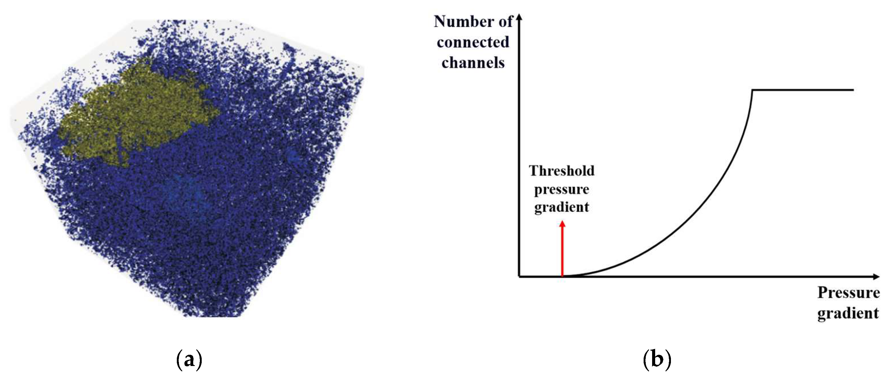
2.1. Analysis of Microscopic Connectivity from Digital Rock Analysis

From a microscopic perspective, an underground reservoir can be regarded as a complex and intricate porous media (Figure 1a). Its internal pore structure not only includes pore size, shape, and spatial distribution but also involves the connectivity and topological relationships between pores. These characteristics constitute the foundational framework of reservoir connectivity and play a decisive role in the large-scale flow characteristics.
In oilfield development, the subsurface fluids begin to migrate within the porous media under pressure difference. This process involves multiple physical and chemical processes, such as the dynamic balance of interfacial forces and the overcoming of capillary forces. As the displacement pressure changes, the number of pore channels involved in fluid flow exhibits high degrees of variability, leading to different flow capabilities [26,27,28]. Specifically, when the applied pressure gradient is at a low level, fluid flow is almost stagnant due to capillary forces within the pore channels. However, as the pressure gradient gradually increases and reaches the threshold pressure gradient, the fluid begins to overcome resistance and initiates flow in some of the pore channels (Figure 1b). With the further increase of the pressure gradient, more and more pore channels are activated, significantly increasing the number of pore channels participating in fluid flow. When the pressure gradient increases to a certain critical value, all pore channels are connected and participate in the fluid flow [29,30,31]. At this point, the flow rate reaches its maximum, and the flow state tends to stabilize, forming a saturated flow state.
The above discussion clearly implies that there is a close relationship between pore-scale connectivity and pressure gradient. It is of great significance to investigate this relationship deeply when analyzing connectivity on a large scale.

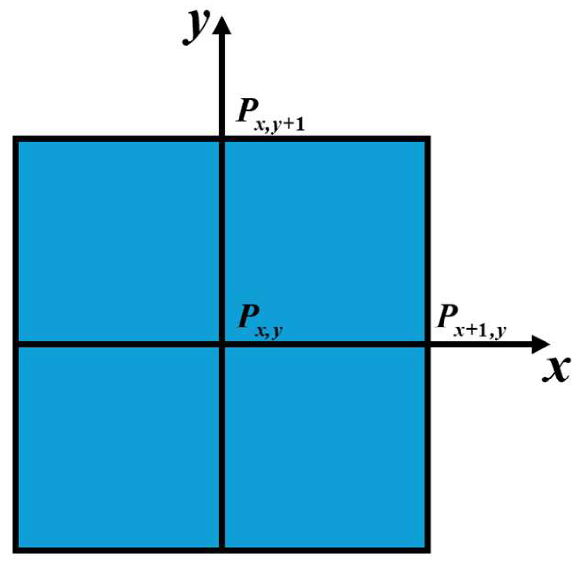
2.2. Establishment of Comprehensive Model for Macroscopic Connectivity Field

Research on microscopic characteristics of fluid flow has revealed a positive correlation between pressure gradient and the number of connected pores. This correlation implies that as the pressure gradient increases, the number of connected pores also rises, thereby enhancing connectivity at the microscopic level. Based on this finding, a quantitative model can be constructed to describe the relationship between pressure gradient and connectivity at a macroscopic scale. By integrating multiple key reservoir parameters, the dynamic field of pressure gradient can be potentially transformed into a dynamic field of connectivity.
As shown in Figure 2, to overcome the effects of flow direction, the magnitude of the pressure gradient is calculated for every well grid cell as follows:
P = ( P x ) 2 + ( P y ) 2 = P x + 1 , y P x , y l 2 + P x , y + 1 P x , y l 2
The micro-level studies have clearly shown a positive correlation between connectivity and pressure gradient. However, in practical applications, relying solely on the isolated parameter of pressure gradient often encounters limitations. As shown in Figure 3a, the conceptual model includes an injection well in the middle and four productions on corners. Heterogeneity is obtained by increasing the permeability between injection wells and the bottom left well. As indicated in Figure 3b, the calculated magnitude of the pressure gradient is low in the high permeable zone. However, the high permeable zone is the area with better connectivity, as proved by the simulated streamlines. This inconsistency clearly shows the discrepancy in using the magnitude of the pressure gradient to represent the connectivity field.
In view of the limitation, more parameters need to be included to better characterize the connectivity of the reservoir. We conduct an in-depth exploration of parameters for representing dynamic connectivity. In this process, a series of key parameters such as permeability, viscosity, and net-to-gross ratio are introduced, aiming to optimize the connectivity model. After this series of analyses, a new representation model for connectivity is proposed with the following formula:
E x , y = k x , y P x + 1 , y P x , y D x 2 + P x , y + 1 P x , y D y 2 × 2 D x × D z + D y × D z × N T G μ o S o S wr / 1 S wr + μ w 1 S o + S wr / 1 S wr
where k x , y is the permeability. P x + 1 , y P x , y D x 2 + P x , y + 1 P x , y D y 2 is the pressure gradient magnitude. 2 D x × D z + D y × D z is the horizontal cross-sectional area of the grid. N T G is the net-to-gross ratio. μ o is the oil viscosity, and μ w is the water viscosity. S o is the oil saturation, and S wr is the irreducible water saturation. μ o S o S wr / 1 S wr + μ w 1 S o + S wr / 1 S wr is the viscosity of mobile mixed fluids.
The newly proposed model acts as a highly integrated evaluation indicator, enabling a more accurate and thorough quantitative evaluation of the dynamic connectivity among grid cells. It introduces a permeability factor for weighting based on the pressure gradient magnitude, aiming to effectively weaken the potential effects of geological heterogeneity on connectivity. Meanwhile, by considering the lateral area of the grid in the horizontal direction, it can accurately reflect the geometric region through which underground fluids pass. The introduction of the net-to-gross ratio further screens out reservoir thicknesses, ensuring the relevance and practicality of the assessment. Additionally, this study further divides the pressure gradient magnitude by the viscosity of mobile fluid in each cell. In this way, we are able to address the complex impact of different oil–water viscosity ratios on connectivity.
Furthermore, from the perspective of dimensional analysis, the pressure gradient magnitude has dimensions of ML−2T−2 (where M represents mass, L represents length, and T represents time). Permeability, on the other hand, has dimensions of L2. The viscosity of mixed fluids has dimensions of ML−1T−1. Additionally, the lateral area of the grid in the horizontal direction has dimensions of L2. Lastly, the net-to-gross ratio, being a proportional parameter, has dimensions of 1, indicating it is a dimensionless quantity. The formula for dimensional analysis is as follows:
E ( Dimension ) = L 2 M L 2 T 2 L 2 1 M L 1 T 1 = L 3 T 1
Based on the above dimensional analysis, the derived representation parameter E has dimensions of L3T−1, which coincides with the dimensions of the volumetric flow rate. Therefore, parameter E not only intuitively reflects the flow rate and scale of fluids within the reservoir but also comprehensively reveals the dynamic connectivity between grid cells during water flooding.

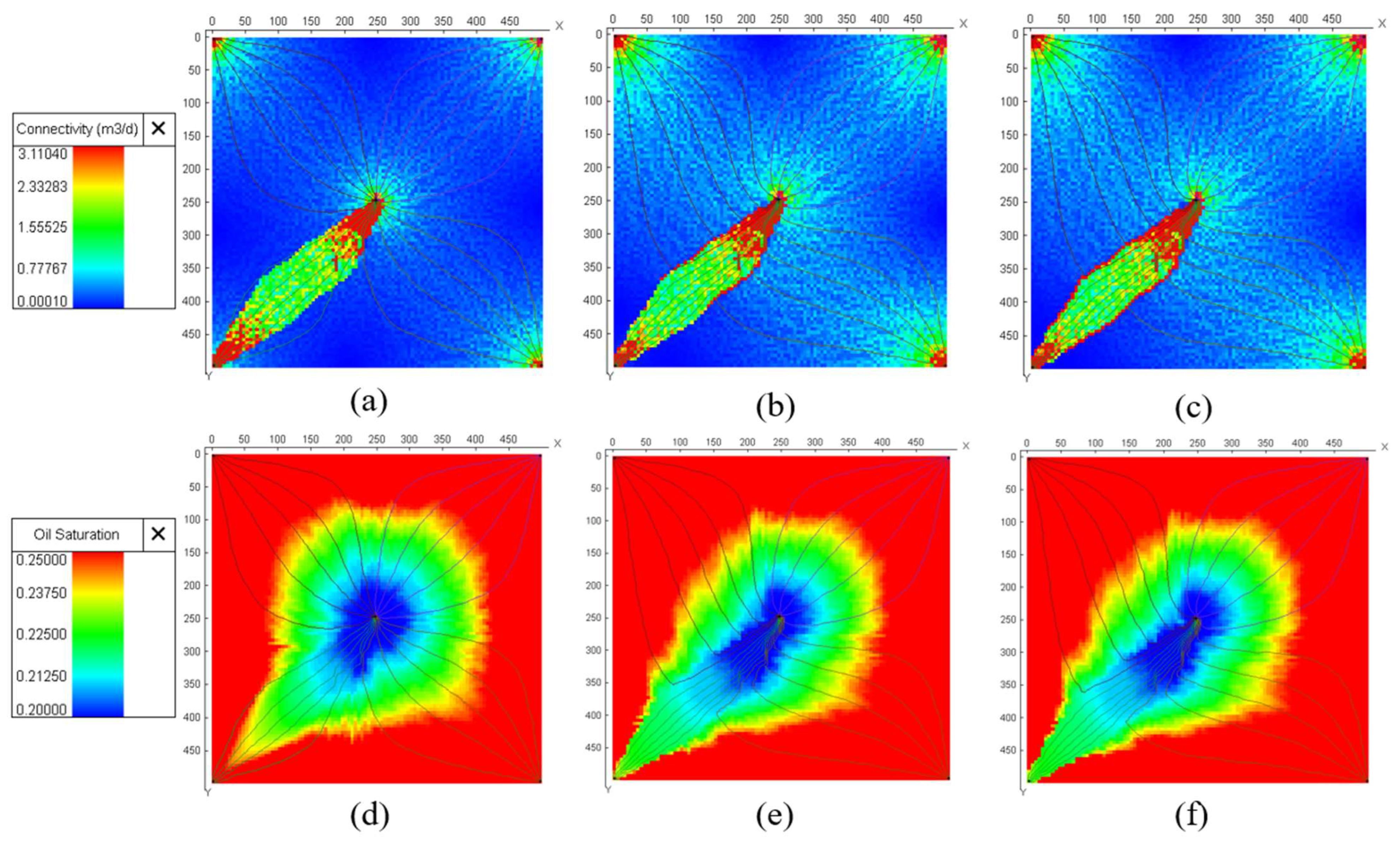
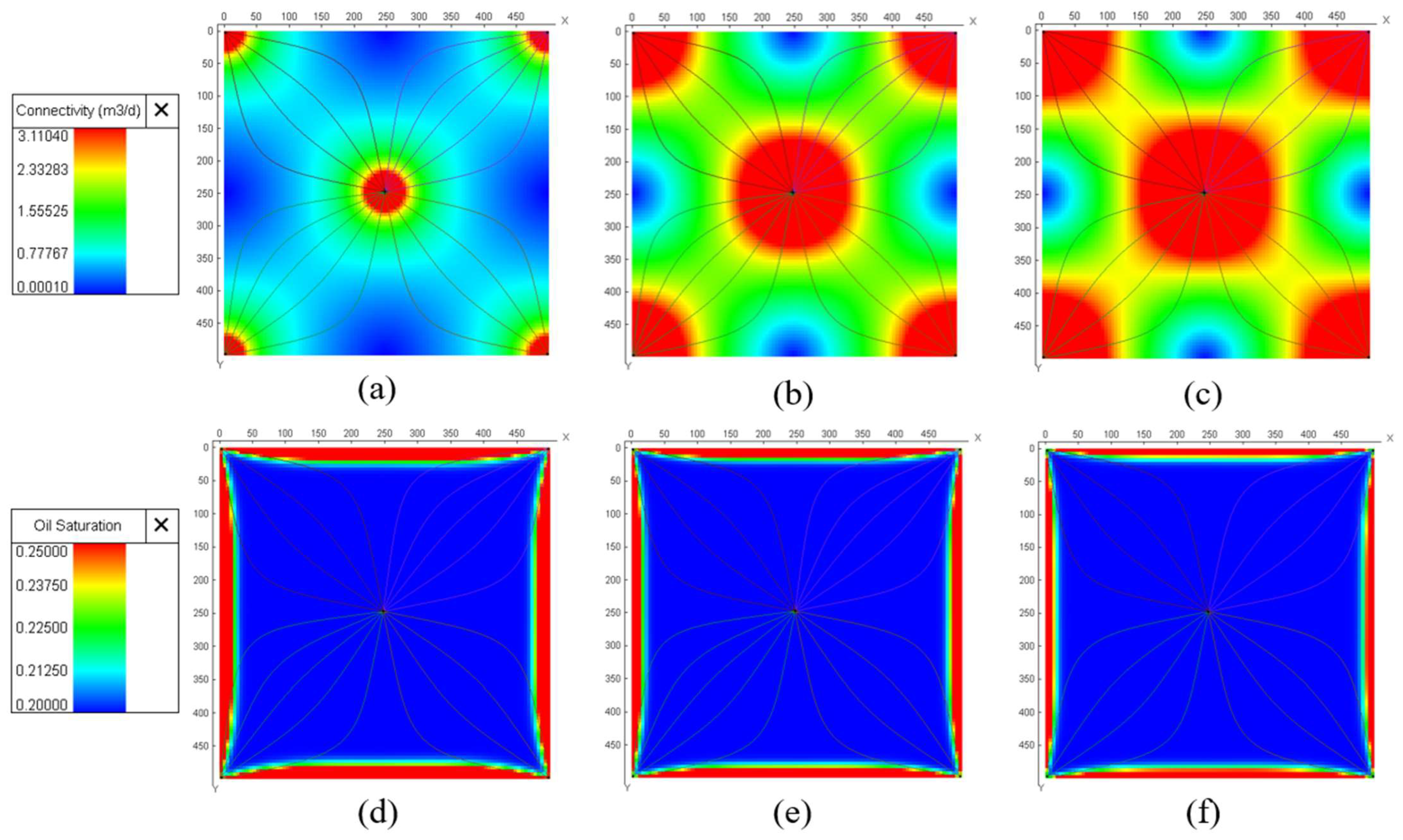
2.3. Validation of the Proposed Model for Connectivity Field

In this part, we validated the proposed connectivity model with streamlines generated from reservoir simulation. A homogeneous model is built in Figure 4, with the same porosity and permeability everywhere. This model is based on the classic design of a five-spot pattern, consisting of one central injection well surrounded by four evenly distributed production wells. Using this model, parameter E is calculated for each grid to quantitatively characterize dynamic connectivity, and subsequently, a map of the dynamic connectivity field is plotted. The connectivity field is then compared with both streamlines and oil saturation, demonstrating a good match (Figure 5). The field maps presented in this study were generated using tNavigator, a reservoir numerical simulation platform that conforms to the principles of mass conservation. The mass conservation equations are as follows:
Oil phase:
[ ρ osc B o ν o ] + q o = t ( ϕ ρ osc B o S o )
Water phase:
[ ρ wsc B w ν w ] + q w = t ( ϕ ρ wsc B w S w )
where t is the time. q o and q w are the mass flow rates of oil and water, respectively. B o and B w are the formation volume factors for oil and water, respectively. ν o and ν w are the flow velocities of oil and water, respectively. ρ osc and ρ wsc are the densities of oil and water, respectively, under standard conditions. S o and S w are the saturations of oil and water, respectively. ϕ is the average porosity of the formation.
Given that both oil and water obey Darcy’s law, the equations of motion considering the time-dependent properties of the formation are as follows:
Oil phase:
ν o = k ro ( F t ) k ( F d ) μ o ( F t ) ( p ρ o g D )
Water phase:
ν w = k rw ( F t ) k ( F d ) μ w ( p ρ w g D )
where F d is the directional displacement flux. k ro and k rw are the relative permeabilities of oil and water, respectively. D is the depth measured from a reference datum. μ o and μ w are the viscosities of the oil and water, respectively. k is the formation permeability. g is the acceleration of gravity. p is the formation pressure.
By substituting the above equations of motion of the two phases of oil and water into their respective mass conservation equations. The permeability equations that account for the time-dependent properties of the formation can be obtained:
Oil phase:
[ k ro ( F t ) k ( F d ) B o μ o ( F t ) ( p ρ o g D ) ] + q vo = t ( φ S o B o )
Water phase:
[ k rw ( F t ) k ( F d ) B w μ w ( p ρ w g D ) ] + q vw = t ( φ S w B w )
where q vo and q vw are the volumetric flow rates of oil and water, and p is the formation pressure.
The formula for calculating oil saturation is as follows:
S o = V o V p
where S o is the oil saturation, V o is the oil phase volume, and V p is the pore volume.
We also investigate how injection rate affects the connectivity field using the proposed model. As shown in Figure 6, when the injection rate increases, the test field map reveals a significant expansion of high-connectivity areas, which is accompanied by a corresponding decrease in oil saturation within these regions. Additionally, streamline density and connectivity field shows a clear positive correlation, with high-connectivity areas featuring denser streamlines. This intuitively reveals that fluids in these areas possess stronger migration capabilities and better connectivity conditions. The experimental results indicate that, under homogeneous reservoir conditions, the utilization of parameter E exhibits excellent applicability for characterizing the dynamic connectivity of the reservoir.
Reservoir heterogeneity is an important factor that affects connectivity. Thus, a heterogeneous model is built for further evaluation. Specifically, the adjustment was made in a specific area of the original homogeneous model, namely the region located between the central injection well and the bottom-left production well. The permeability in this area (denoted as k1) was increased, while the permeability in the remaining areas of the model (denoted as k2) remained constant. As the permeability ratio k1/k2 gradually increased, the distribution density of streamlines within the high-permeability area (k1 area) also intensified (Figure 7). This change was accompanied by a corresponding decrease in oil saturation within this area. Simultaneously, regions of high connectivity also expand. This finding demonstrates that the model for the dynamic connectivity field is effective and accurate in describing fluid flow and connectivity in heterogeneous reservoirs.
Based on a homogeneous model, we also conducted tests by varying the oil–water viscosity ratio (denoted as μo/μw) to simulate different polymer flooding conditions, as illustrated in Figure 8. It was observed that as the oil–water viscosity ratio decreases, the high connectivity field area expands. Throughout this process, the connectivity field is positively correlated with the density of streamlined distribution and negatively correlated with oil saturation. This demonstrates the model can represent the impact of polymer flooding on connectivity.
The proposed model for the connectivity field using parameter E has demonstrated good performance under both homogeneous and heterogeneous reservoir conditions. The model precisely defines high-connectivity areas through quantitative analysis, which exhibit good consistency with regions of high-density distribution of streamlines, as well as low oil saturation. This outcome fully confirms the broad applicability and high accuracy of the model for the dynamic connectivity field.

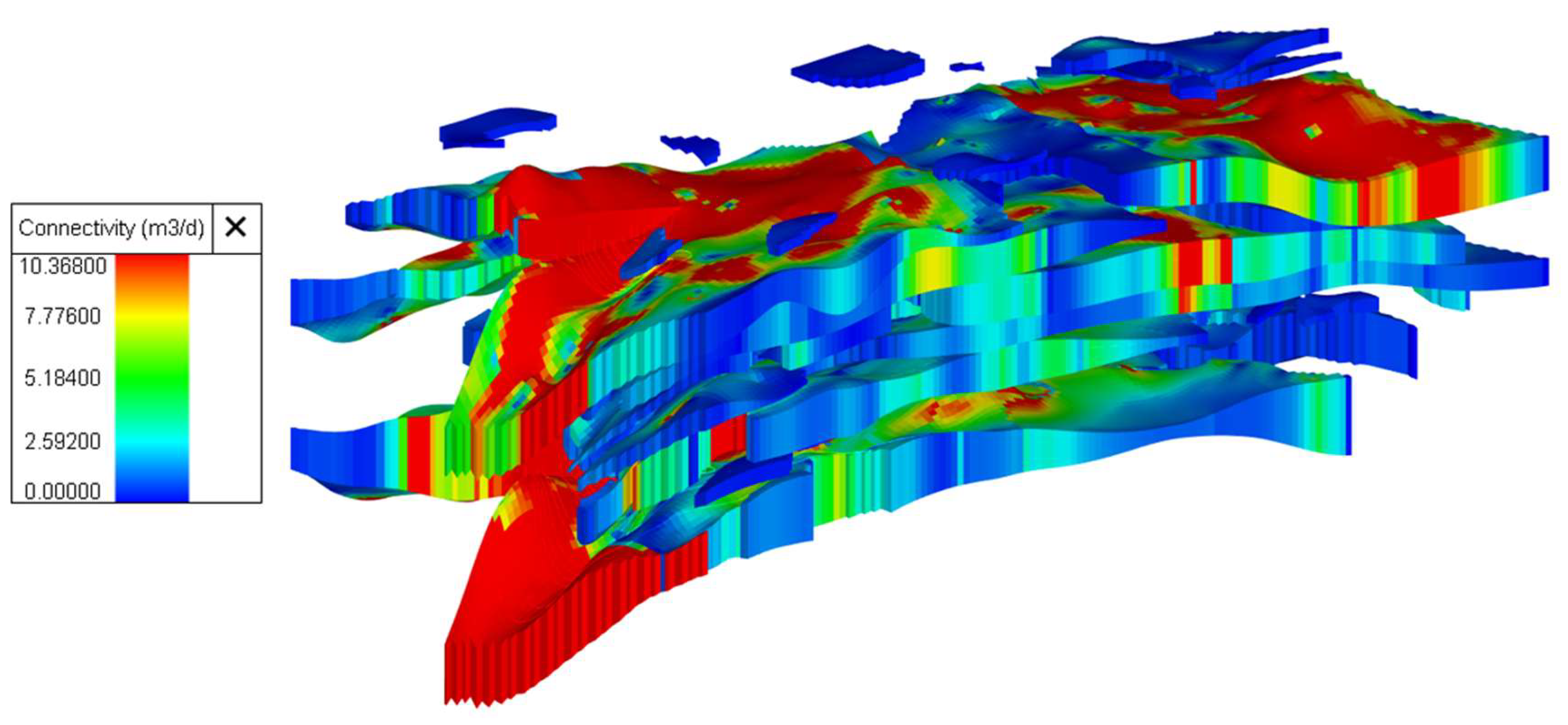
3. Analysis of Connectivity Field in an Offshore Reservoir Using Proposed Method

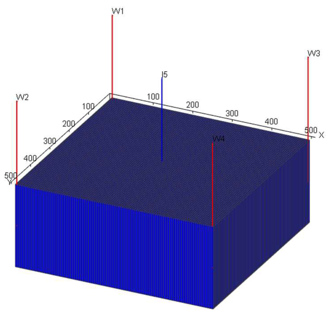
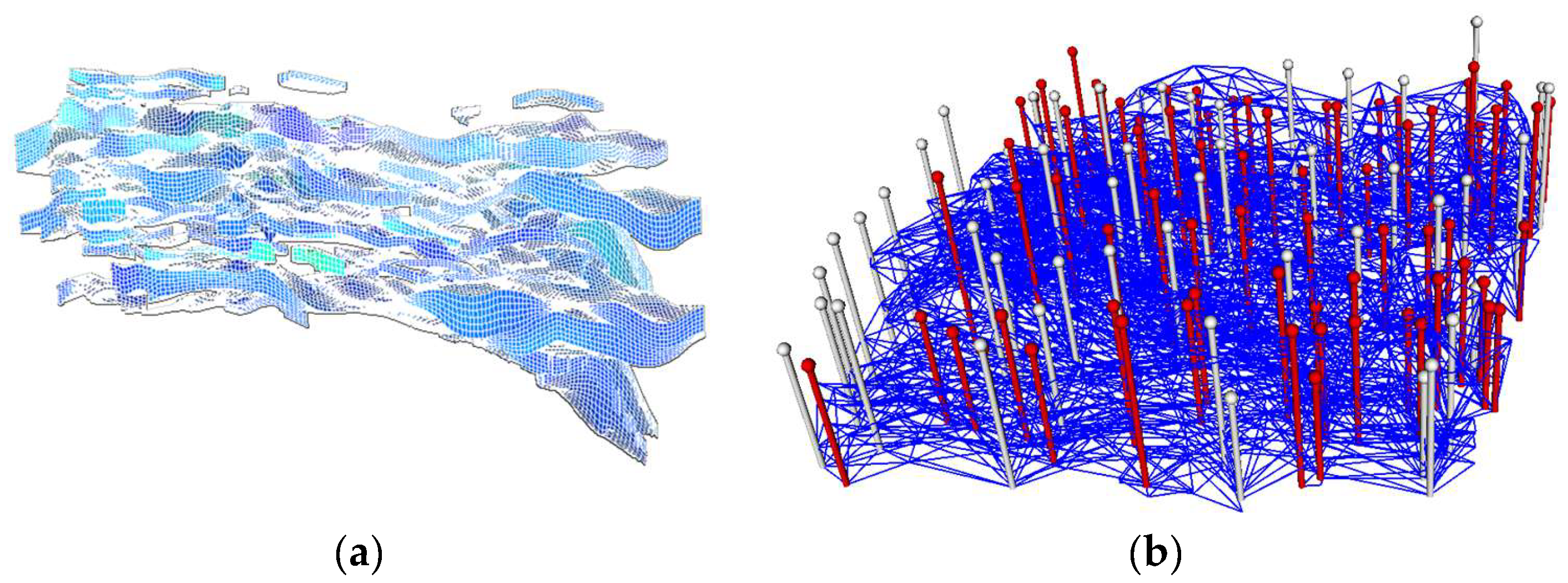
3.1. Establishment of a Three-Dimensional Dynamic Connectivity Field Model

In this part, we apply the model of the connectivity field in an offshore reservoir. The reservoir is a monocline structure, higher in the east and lower in the west, with a structural relief of approximately 40 m and a dip angle of 2°. The target oil layer is formation A at depths of 1180–1300 m. It covers 3.6 km2 with an effective thickness of 15.1 m and geological reserves of 9.516 mt. The reservoir can be divided into nine sublayers vertically, with the third and ninth layers as the main layers. As of July 2023, the unit has 44 production wells and 28 injection wells. The daily liquid production rate per well is 89.4 t (2.1 t oil), with 100 m3/d water injection. The recovery factor is 50.5%, and the average water cut is 97.6%, indicating a “double-high” stage of high water cut and high recovery.
Due to the complex connectivity of this reservoir, the water–oil displacement within the reservoir is uneven both vertically and laterally. Therefore, accurately describing the connectivity field and clarifying its three-dimensional connectivity has become the foundation for studying the distribution of remaining oil. To better analyze the connectivity, the grid-based reservoir (Figure 9a) is transformed into a connection network consisting of connectivity elements [32]. Firstly, characteristic points from the grid model are filtered, including well locations, boundaries, fractures, etc. In this way, a points cloud is constructed for the reservoir. Then, each point is assigned an influence domain. By connecting the point with other points inside the domain, connections between points are constructed. Each line between points is called a connection element. The connection elements are characterized by two parameters: connection transmissibility (T) and connection volume (V). Connection transmissibility describes the flow capacity between two points, and connection volume represents the control volume of two points. This process effectively transforms the traditional grid model into a more flexible and efficient connectivity element model (Figure 9b). It improves simulation accuracy and efficiency while preserving original geological characteristics.
Based on the selected well locations and reservoir properties, the connectivity element model for this reservoir is established. In the vertical structure of the model, it is meticulously divided into nine layers. For the inter-well connection method, a modeling approach based on the linear connection of the point cloud has been adopted. This scheme accurately captures the spatial relationships between well locations using point cloud technology and employs linear connections to construct a connectivity model among wells. Figure 10 presents the constructed connection element model for layer 3, with the left presenting connection transmissibility and the right presenting connection volume.
A history-matching procedure was then performed on the established connectivity model to invert the characteristic parameters. In this process, the cumulative oil production of the selected block was designated as the objective function. Through a meticulous optimization algorithm, systematic corrections were made to the two key characteristic parameters: connection transmissibility and connection volume. The historical matching results for the block are illustrated in Figure 11. Clearly, there is a good match between simulated results and observed production data.
The formula for calculating field water cut is as follows:
W c = Q w Q t × 100 %
where W c is the field water cut, Q w is the volume flow rate of the produced water, and Q t is the volume flow rate of the produced fluid.
The formula for field oil production is as follows:
N p = i = 1 n Q o , i × Δ t i
where N p is the field oil production, Q o , i is the oil production during the i-th time interval, Δ t i is the length of the i-th time interval, and n is the total number of time intervals.
In addition, for the connectivity model, history matching was also adopted to invert characteristic parameters for each well. The historical matching results for the individual wells are illustrated in Figure 12. The good match further confirms the validity and accuracy of the model.
After history matching, the accurate pressure field is obtained for the whole reservoir. Combined with other key parameters such as permeability, saturation and viscosity, the connectivity field can be calculated using the proposed model in Equation (2). The 3D dynamic connectivity field for the offshore reservoir is illustrated in Figure 13. The model allows for a more accurate prediction of fluid distribution, flow paths, and production potential within the reservoir. Consequently, it enables the formulation of more scientific strategies for water flooding, thereby maximizing the reservoir’s production rate and economic benefits.

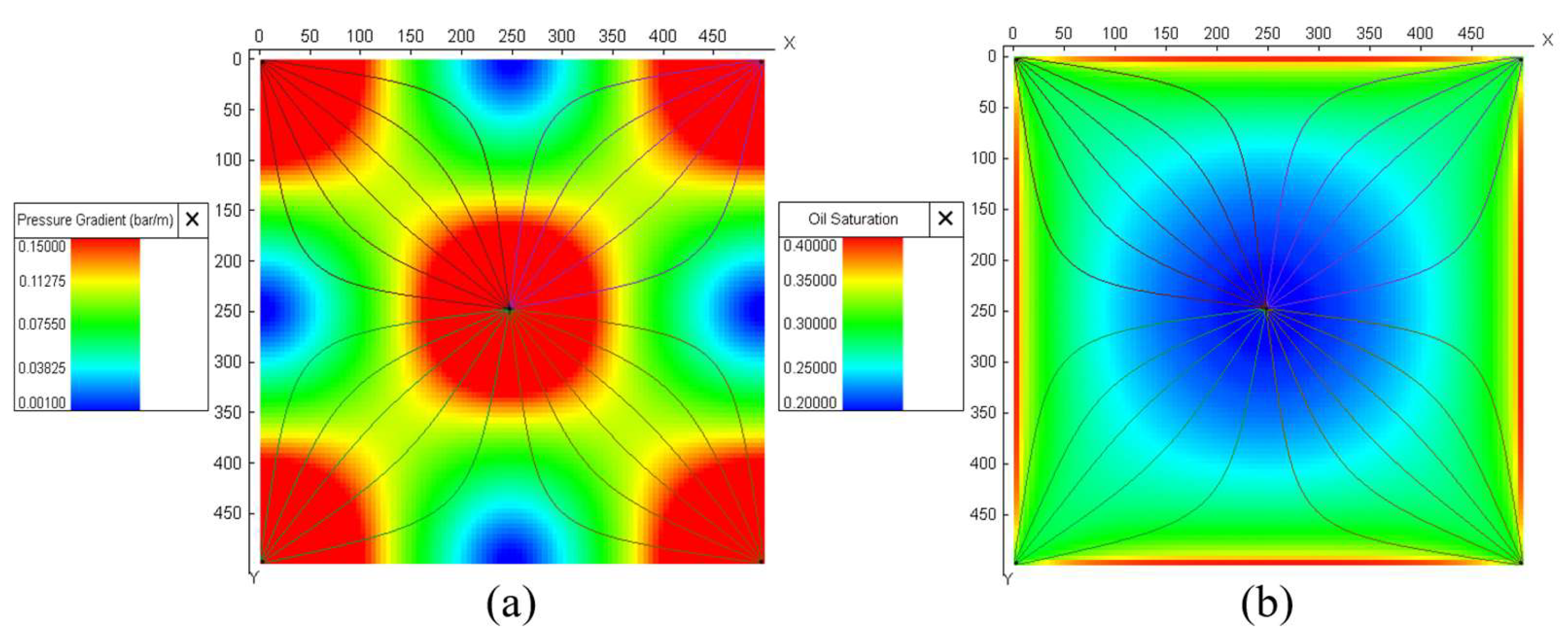
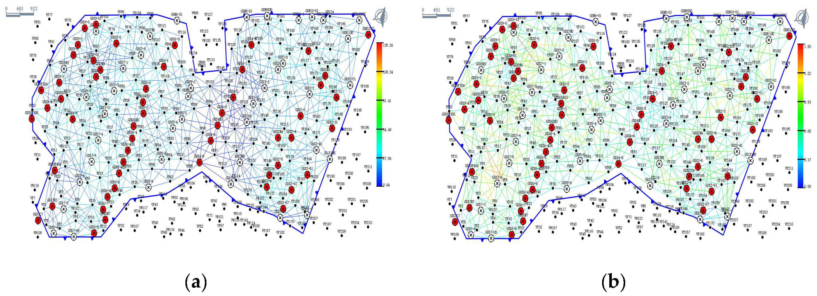
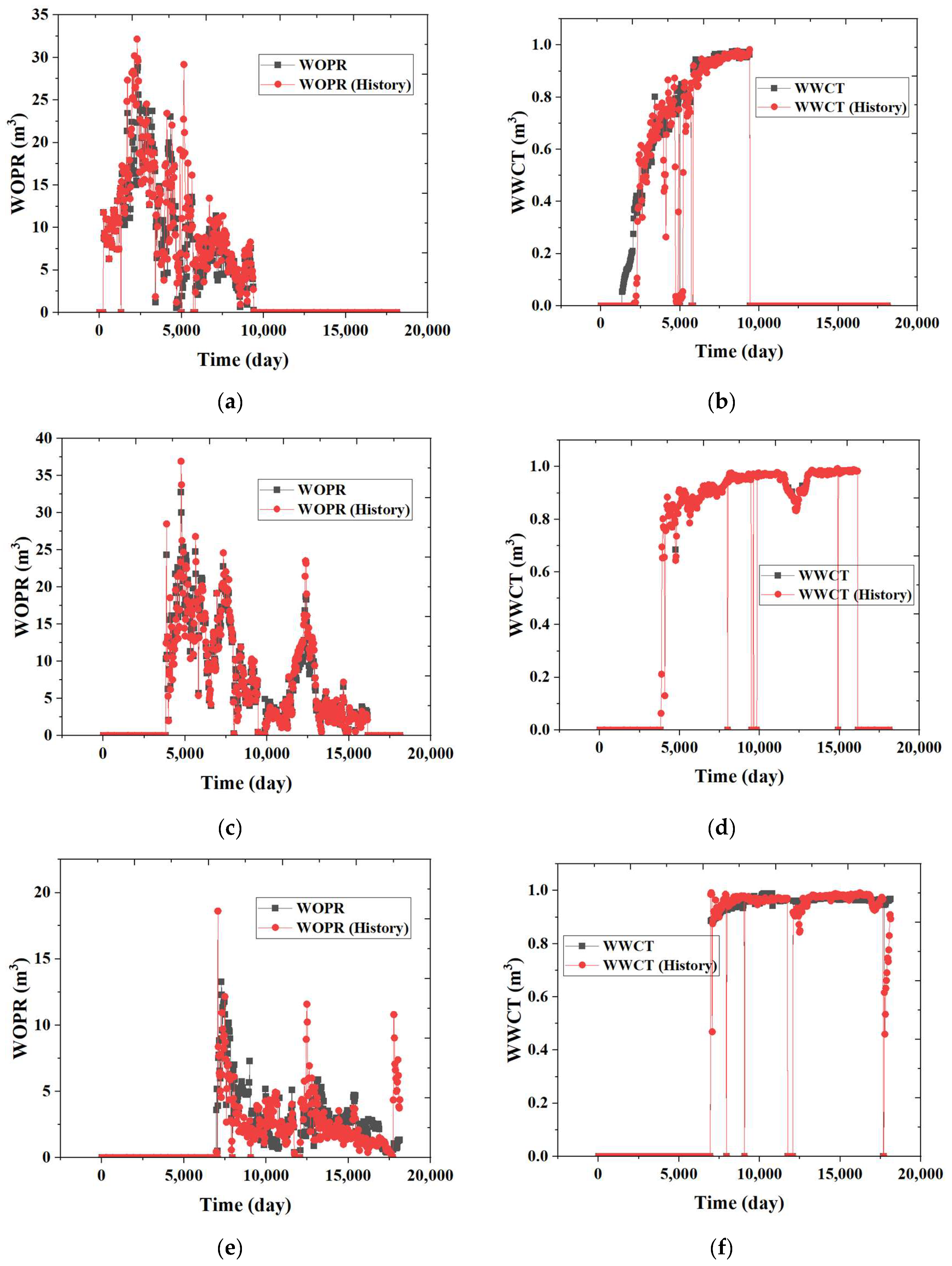
3.2. Comparisons Between Connectivity Field with On-Site Data
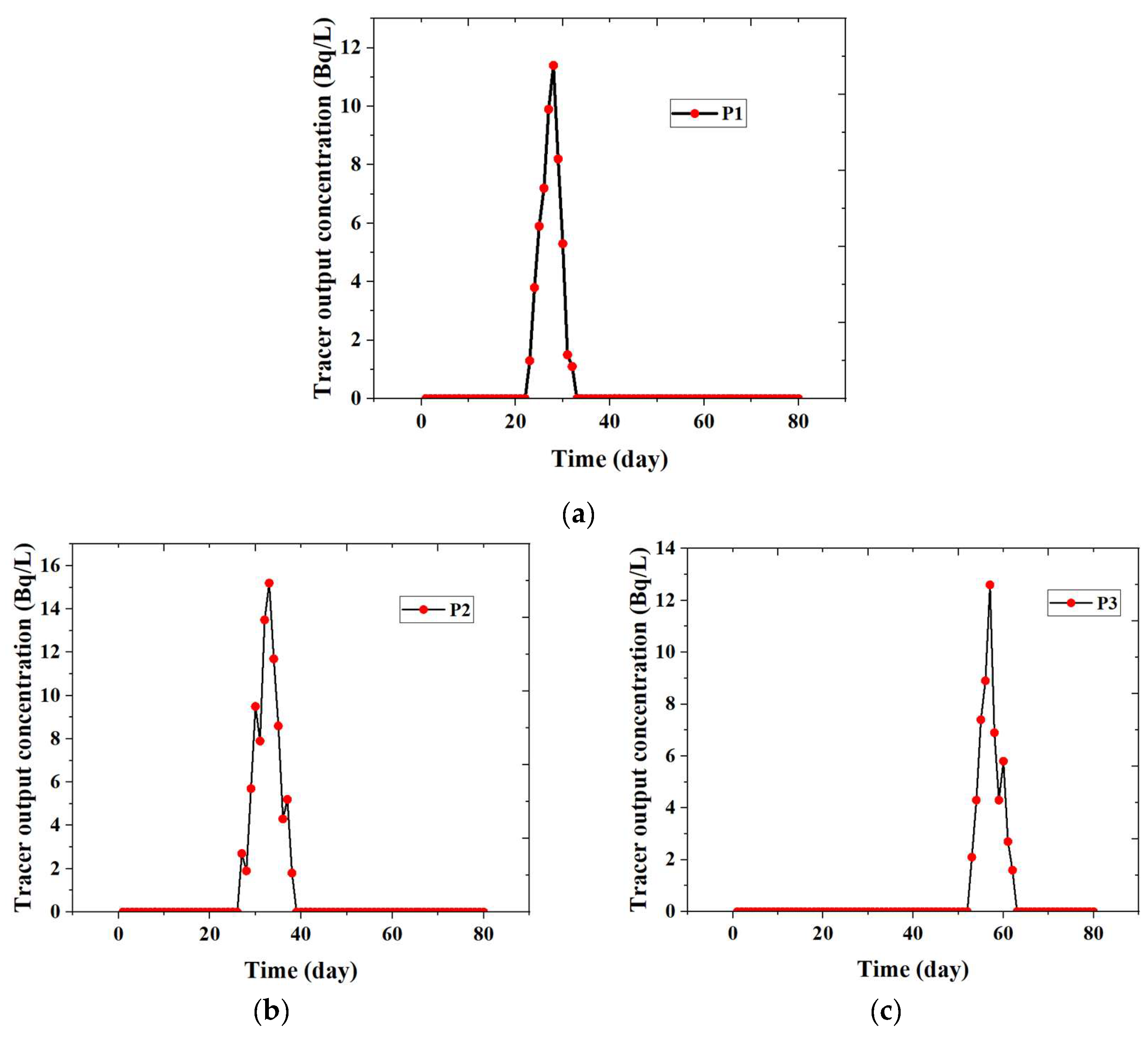
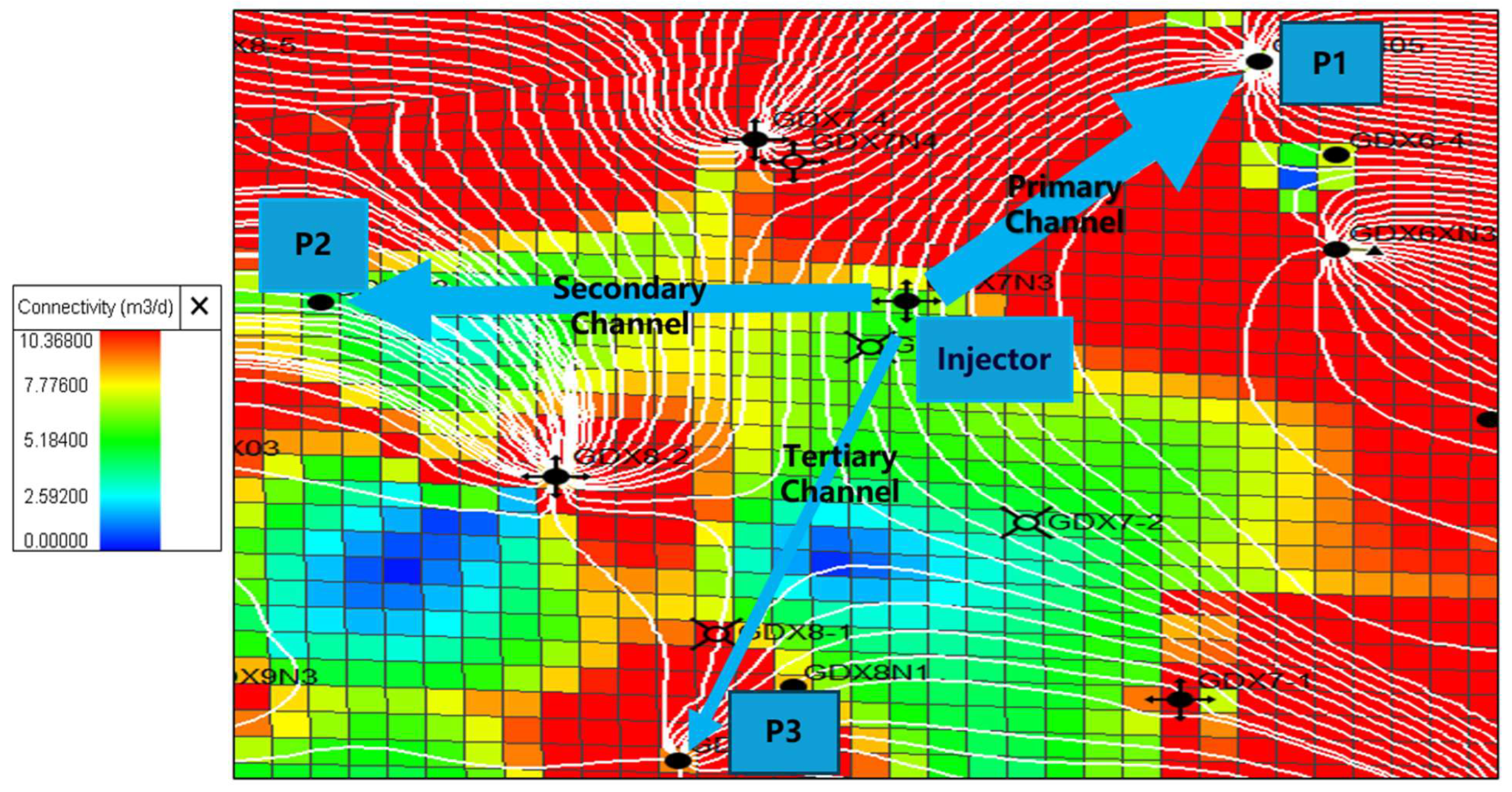
A.
Comparison with the Tracer Test
An on-site tracer test was conducted in the third layer (main layer) in September 2022, in well group P. A comparison between the calculated connectivity field and the results of the tracer test is conducted. The tracer detection results (Figure 14) for well group P are as follows: The tracer response at production well P1 is the fastest, indicating excellent connectivity in this layer, which aligns with the dynamic connectivity field established in this work. The tracer response at production well P2 is slightly slower but still demonstrates good injection–production correspondence and connectivity, consistent with the model’s predictions. At production well P3, tracer response is observed with a longer detection time, suggesting relatively weaker connectivity, which also matches the dynamic connectivity field (Figure 15). The tracer verification results are summarized in Table 1.
The response speed of tracers in production wells accurately reflects the connectivity in the reservoir. This consistency with the predictions from the dynamic connectivity field validates the accuracy of the model.
B.
Comparison with splitting coefficient of injected water
In oilfield applications, an injection well is often connected to multiple production wells, creating a network of flow paths. The splitting coefficient, denoted as S i , j , quantifies the fraction of injected fluid from a specific injection well i that reaches a connected production well j. This dimensionless parameter (0 ≤ S i , j ≤ 1) reflects the positive correlation between splitting coefficients and connectivity within the injection–production pair. The splitting coefficient can be calculated using the transmissibility and pressure difference between the wells. The formula is as follows:
S i , j n = q i , j n q i n = T i , j n ( p j n p i n ) j = 1 N T i , j n ( p j n p i n )
where S i , j n is the splitting coefficient from well i to well j. q i , j n is the split fluid volume from well i to well j, and q i n is the total fluid volume injected by well i. T i , j n is the transmissibility from well i to well j. ( p j n p i n ) is the pressure difference between well i and well j. Superscript N is the number of production wells connected to well I, and superscript n is the time step corresponding to index n.
Due to the intimate relationship between splitting coefficients and connectivity, we utilized splitting coefficients to validate the reliability of established dynamic connectivity fields by overlaying the dynamic connectivity fields of the main layers (the third layer and the ninth layer) with the splitting coefficients of the injection well (Figure 16). We can observe a positive correlation between the splitting direction and the connectivity field. Specifically, areas with clear splitting directions exhibit a larger connectivity field, and an increase in splitting coefficients is accompanied by a further enlargement of the connectivity field. This finding effectively confirms the high accuracy of the representation method for dynamic connectivity fields presented in this work.

4. Conclusions

This study integrates multiple key factors influencing dynamic connectivity and constructs a mathematical model to describe the connectivity field. The model can handle the effects of permeability heterogeneity, injection rates and viscosity ratio on connectivity. The model is first validated in a conceptual model by comparing simulated connectivity fields with streamlines. Then, the proposed model is applied to construct the 3D connectivity field for an offshore reservoir. By converting the grid-based reservoir model into the connection element model, the connectivity field is constructed in an efficient manner. Comparison with results of the tracer test and water splitting factor further proves the accuracy of the proposed method. The model of the connectivity field shows promise in analyzing the connectivity for the whole reservoir. It helps enhance the efficiency of water injection and optimize offshore reservoir management.

Author Contributions

Conceptualization, F.D. and H.Z.; methodology, Y.H. and C.G.; software, L.T. and M.C.; validation, Y.H. and C.G.; formal analysis, M.C.; investigation, F.M.; resources, F.M.; data curation, H.Z.; writing—original draft preparation, Y.H. and C.G.; writing—review and editing, F.D.; visualization, M.C.; supervision, F.D.; funding acquisition, F.D. All authors have read and agreed to the published version of the manuscript.

Funding

This research was funded by the National Natural Science Foundation of China grant number No. 52204026.

Data Availability Statement

Data is contained within the article.

Conflicts of Interest

Author Li Tao was employed by the Exploration and Development Research Institute, Sinopec Shengli Oilfield Company. The remaining authors declare that the research was conducted in the absence of any commercial or financial relationships that could be construed as a potential conflict of interest.

References

  1. Moyen, R.; Doyen, P.M. Reservoir connectivity uncertainty from stochastic seismic inversion. In SEG Technical Program Expanded Abstracts 2009; Society of Exploration Geophysicists: Tulsa, Ok, USA, 2009; pp. 2378–2382. [Google Scholar]
  2. Ragagnin, G.M.; Moraes, M.A.S. Seismic geomorphology and connectivity of deepwater reservoirs. SPE Reserv. Eval. Eng. 2008, 11, 686–695. [Google Scholar] [CrossRef]
  3. Riazi, N.; Clarkson, C.R. The importance of seismic attributes in reservoir characterization and inter-well connectivity studies of tight oil reservoirs. In Proceedings of the Geoconvention 2016, Calgary, AB, Canada, 7–11 March 2016. [Google Scholar]
  4. Van-Dunem, F.; Contreiras, K.D.; Weinheber, P.; Rueda, M. Evaluating Reservoir Connectivity and Compartmentalization Using a Combination of Formation Tester and NMR Data. In Proceedings of the SPWLA 49th Annual Logging Symposium, Austin, TX, USA, 25–28 May 2008. [Google Scholar]
  5. Azari, M.; Hadibeik, H.; Eyuboglu, S.; Jambunathan, V.; Khan, W.; Ramakrishna, S.; Haack, J.; Bargas, C.; Khan, M. Using Wireline Formation-Tester Data for Reservoir Characterization and Connectivity Determination in Ultradeepwater and High-Pressure Wilcox Formation in Gulf of Mexico. In Proceedings of the SPE Annual Technical Conference and Exhibition, San Antonio, TX, USA, 9–11 October 2017. [Google Scholar]
  6. Sanni, M.; Abbad, M.; Kokal, S.; Ali, R.; Zefzafy, I.; Hartvig, S.; Huseby, O. Reservoir description insights from an inter-well chemical tracer test. In Proceedings of the SPE Kingdom of Saudi Arabia Annual Technical Symposium and Exhibition, Dammam, Saudi Arabia, 24–27 April 2017. [Google Scholar]
  7. Sanni, M.L.; Al-Abbad, M.A.; Kokal, S.L.; Hartvig, S.; Olaf, H.; Jevanord, K. A field case study of inter-well chemical tracer test. In Proceedings of the SPE International Conference on Oilfield Chemistry, The Woodlands, TX, USA, 13–15 April 2015. [Google Scholar]
  8. Al-Qasim, A.; Kokal, S.; Hartvig, S.; Huseby, O. Reservoir description insights from inter-well gas tracer test. In Proceedings of the Abu Dhabi International Petroleum Exhibition and Conference, Abu Dhabi, United Arab Emirates, 11–14 November 2019. [Google Scholar]
  9. Meister, M.; Lee, J.; Krueger, V.; Georgi, D.; Chemali, R. Formation pressure testing during drilling: Challenges and benefits. In Proceedings of the SPE Annual Technical Conference and Exhibition, Denver, CO, USA, 5–8 October 2003. [Google Scholar]
  10. Hahne, U.; Kaniappan, A.; Pragt, J.; Buysch, A. LWD formation pressure testing allows decision making while drilling. In Proceedings of the IADC/SPE Asia Pacific Drilling Technology Conference and Exhibition, Bangkok, Thailand, 13–15 November 2006. [Google Scholar]
  11. Almasoodi, M.; Andrews, T.; Johnston, C.; Singh, A.; McClure, M. A new method for interpreting well-to-well interference tests and quantifying the magnitude of production impact: Theory and applications in a multi-basin case study. Geomech. Geophys. Geo-Energy Geo-Resour. 2023, 9, 95. [Google Scholar] [CrossRef]
  12. Ohaeri, C.U.; Sankaran, S.; Fernandez, J. Evaluation of reservoir connectivity and hydrocarbon resource size in a deep water gas field using multi-well interference tests. In Proceedings of the SPE Annual Technical Conference and Exhibition, Amsterdam, The Netherlands, 27–29 October 2014. [Google Scholar]
  13. Aref, E.; Jahangiri, H.R. Data Driven Approach to Infer Inter-well Connectivity among Production Wells in an Oil Synthetic Reservoir. J. Pet. Res. 2021, 31, 40–53. [Google Scholar]
  14. Hird, K.B.; Dubrule, O. Quantification of reservoir connectivity for reservoir description applications. SPE Reserv. Eval. Eng. 1998, 1, 12–17. [Google Scholar] [CrossRef]
  15. Alabert, F.G.; Modot, V. Stochastic models of reservoir heterogeneity: Impact on connectivity and average permeabilities. In Proceedings of the SPE Annual Technical Conference and Exhibition, Washington, DC, USA, 4–7 October 1992. [Google Scholar]
  16. Malik, Z.A.; Silva, B.A.; Brimhall, R.M.; Wu, C.H. An integrated approach to characterize low-permeability reservoir connectivity for optimal waterflood infill drilling. In Proceedings of the SPE Rocky Mountain Petroleum Technology Conference/Low-Permeability Reservoirs Symposium, Denver, CO, USA, 26–28 April 1993. [Google Scholar]
  17. Canas, J.A.; Malik, Z.A.; Wu, C.H. Use of Hydraulic Interwell Connectivity Concepts in Reservoir Characterization. In Proceedings of the SPE Permian Basin Oil and Gas Recovery Conference, Midland, TX, USA, 16–18 March 1994. [Google Scholar]
  18. Heffer, K.J.; Fox, R.J.; McGill, C.A.; Koutsabeloulis, N.C. Novel techniques show links between reservoir flow directionality, earth stress, fault structure and geomechanical changes in mature waterfloods. SPE J. 1997, 2, 91–98. [Google Scholar] [CrossRef]
  19. Soeriawinata, T.; Kelkar, M. Reservoir management using production data. In Proceedings of the SPE Oklahoma City Oil and Gas Symposium/Production and Operations Symposium, Oklahoma City, OK, USA, 28–31 March 1999. [Google Scholar]
  20. Albertoni, A.; Lake, L.W. Inferring interwell connectivity only from well-rate fluctuations in waterfloods. SPE Reserv. Eval. Eng. 2003, 6, 6–16. [Google Scholar] [CrossRef]
  21. Yousef, A.A.; Gentil, P.; Jensen, J.L.; Lake, L.W. A capacitance model to infer interwell connectivity from production-and injection-rate fluctuations. SPE Reserv. Eval. Eng. 2006, 9, 630–646. [Google Scholar] [CrossRef]
  22. Yousef, A.A.; Lake, L.W.; Jensen, J.L. Analysis and interpretation of interwell connectivity from production and injection rate fluctuations using a capacitance model. In Proceedings of the SPE Improved Oil Recovery Conference, Tulsa, Ok, USA, 22–26 April 2006. [Google Scholar]
  23. Yousef, A.A.; Jensen, J.L.; Lake, L.W. Lake. Integrated interpretation of interwell connectivity using injection and production fluctuations. Math. Geosci. 2009, 41, 81–102. [Google Scholar] [CrossRef]
  24. Zhao, H.; Li, Y.; Gao, D.; Cao, L. Research on reservoir interwell dynamic connectivity using systematic analysis method Acta Pet. Sin. 2010, 31, 633–636. [Google Scholar]
  25. Li, F.; Lei, X.; Zhang, Q.; Cha, Y.; Sun, S. A new technique for characterization of reservoir connectivity based on CT scanning. Petrochem. Ind. Appl. 2019, 38, 74–81+88. [Google Scholar]
  26. Deng, Y.; Liu, S.; Ma, C. Integrated Analysis Methods for Inter-Well Connectivity. Fault-Block Oil Gas Field 2003, 10, 50–53. [Google Scholar]
  27. Tang, L.; Yin, Y.; Zhang, G. Study on Connectivity of Injection-Production Systems. J. Oil Gas Technol. 2008, 30, 134–136. [Google Scholar]
  28. Wang, H.; Wang, L.; Liu, H.; Liu, J.; Liu, W.; Shen, C. Analysis of Fluvial Sand Connectivity with Production and Seismic Data. Offshore Oil 2014, 34, 66–71. [Google Scholar]
  29. Zahm, C.K.; Zahm, L.C.; Bellian, J.A. Integrated fracture prediction using sequence stratigraphy within a carbonate fault damage zone, Texas, USA. J. Struct. Geol. 2010, 32, 1363–1374. [Google Scholar] [CrossRef]
  30. Fabuel-Perez, I.; Hodgetts, D.; Redfern, J. Integration of digital outcrop models (DOMs) and high resolution sedimentology–workflow and implications for geological modelling: Oukaimeden Sandstone Formation, High Atlas (Morocco). Pet. Geosci. 2010, 16, 133–154. [Google Scholar] [CrossRef]
  31. Yan, J.; Liang, Q.; Geng, B.; Lai, F.; Wen, D.; Wang, Z. Relationship between micro-pore characteristics and pore structure of lowpermeability sandstone: A case of the fourth member of ShahejieFormation in southern slope of Dongying Sag. Lithol. Pet. Reserv. 2017, 29, 18–26. [Google Scholar]
  32. Zhao, H.; Liu, W.; Rao, X.; Zhan, W.; Li, Y. Reservoir Numerical Simulation Using Connectivity Element Method. Sci. China Technol. Sci. 2022, 52, 1869–1886. [Google Scholar]
Figure 1. 3D Digital core model with connected channels variation. (a) 3D digital core model generated via CT scanning [25]. (b) Diagram of the variation in the number of connected channels.
Jmse 13 00906 g001
Figure 2. Illustration of two-dimensional pressure along a grid.
Jmse 13 00906 g002
Figure 3. Superposed field of pressure gradient and streamline distribution under heterogeneous condition. (a) Permeability field (b) Pressure gradient field.
Jmse 13 00906 g003
Figure 4. Conceptual reservoir model with well locations.
Jmse 13 00906 g004
Figure 5. Comparison of connectivity field with simulated streamlines and oil saturation. (a) Connectivity field (b) Oil saturation field.
Jmse 13 00906 g005
Figure 6. Effect of injection rate on dynamic connectivity field. Effect of heterogeneity on connectivity field. (a) Connectivity field (Injection rate: 60 m3/d) (b) Connectivity field (Injection rate: 160 m3/d) (c) Connectivity field (Injection rate: 200 m3/d) (d) Oil saturation (Injection rate: 60 m3/d) (e) Oil saturation (Injection rate: 160 m3/d) (f) Oil saturation (Injection rate: 200 m3/d).
Jmse 13 00906 g006
Figure 7. Effect of heterogeneity on connectivity field. (a) Connectivity field (k1/k2 = 3) (b) Connectivity field (k1/k2 = 50) (c) Connectivity field (k1/k2 = 500) (d) Oil saturation (k1/k2 = 3) (e) Oil saturation (k1/k2 = 50) (f) Oil saturation (k1/k2 = 500).
Jmse 13 00906 g007
Figure 8. Effect of oil–water viscosity ratio on connectivity field. (a) Connectivity field (μow = 10) (b) Connectivity field (μow = 1) (c) Connectivity field (μow = 0.1) (d) Oil saturation (μow = 10) (e) Oil saturation (μow = 1) (f) Oil saturation (μow = 0.1).
Jmse 13 00906 g008
Figure 9. Conversion of the grid model to the connectivity element model. (a) grid model (b) Connectivity element model (red represents oil wells, white represents water wells, and bule represents connectivity paths).
Jmse 13 00906 g009
Figure 10. Reservoir properties parameter field map of the main reservoir layer. (red circles represent oil wells, white circles represent water wells and black dots represent virtual well) (a) Connection conductivity distribution field (b) Connection volume distribution field.
Jmse 13 00906 g010
Figure 11. Results of historical matching for the reservoir block. (a) Field water cut (b) Field oil production.
Jmse 13 00906 g011
Figure 12. Results of historical matching for individual wells. (a) Well oil production rate (well 1) (b) Well water cut (well 1) (c) Well oil production rate (well 2) (d) Well water cut (well 2) (e) Well oil production rate (well 3) (f) Well water cut (well 3).
Jmse 13 00906 g012
Figure 13. Three-dimensional dynamic connectivity field of the offshore reservoir.
Jmse 13 00906 g013
Figure 14. Tracer test results of well group P. (a) The tracer test result of P1 (b) The tracer test result of P2 (c) The tracer test result of P3.
Jmse 13 00906 g014
Figure 15. The superimposed diagram of dynamic connectivity field and streamline distribution of well group P.
Jmse 13 00906 g015
Figure 16. Overlay map of dynamic connectivity field and splitting coefficient of injection well in the main layers. (a) Overlay map of splitting coefficients for the 3rd layer. (b) Overlay map of splitting coefficients for the 9th layer.
Jmse 13 00906 g016
Table 1. Tracer verification results for well group P.
Injection WellProduction WellsTracer Detection SituationWhether It CorrespondsAccuracy
PP1Preferential tracer detection (23 days)Yes100%
P2Tracer detected after 27 daysYes
P3Tracer detected after 53 daysYes
Disclaimer/Publisher’s Note: The statements, opinions and data contained in all publications are solely those of the individual author(s) and contributor(s) and not of MDPI and/or the editor(s). MDPI and/or the editor(s) disclaim responsibility for any injury to people or property resulting from any ideas, methods, instructions or products referred to in the content.

